A comparative study of the unscented Kalman filter and particle filter estimation methods for the measurement of the road adhesion coefficient

The measurement of the road adhesion coefficient is of great significance for the vehicle active safety control system and is one of the key technologies for future autonomous driving. With a focus on the problems of interference uncertainty and system nonlinearity in the estimation of the road adhesion coefficient, this work adopts a vehicle model with 7 degrees of freedom (7-DOF) and the Dugoff tire model and uses these models to estimate the road adhesion coefficient in real time based on the particle filter (PF) algorithm. The estimations using the PF algorithm are verified by selecting typical working conditions, and they are compared with estimations using the unscented Kalman filter (UKF) algorithm. Simulation results show that the road adhesion coefficient estimator error based on the UKF algorithm is less than 7 %, whereas the road adhesion coefficient estimator error based on the PF algorithm is less than 0.1 %. Thus, compared with the UKF algorithm, the PF algorithm has a higher accuracy and control effect with respect to estimating the road adhesion coefficient under different road conditions. In order to verify the robustness of the road adhesion coefficient estimator, an automobile test platform based on a four-wheel-hub-motor car is built. According to the experimental results, the estimator based on the PF algorithm can realize the road surface identification with an error of less than 1 %, which verifies the feasibility and effectiveness of the algorithm with respect to estimating the road adhesion coefficient and shows good robustness.

1 Introduction

With the development of the automobile industry and the increase in car ownership, the rate of road traffic accidents is also increasing. The difficulty involved with obtaining information regarding people and vehicles during driving has become one of the most important factors affecting traffic safety and obscuring the cause of many traffic accidents. In order to ensure the stability of vehicles under critical conditions, anti-lock braking (ABS) systems, accelerated anti-slip regulation (ASR) systems and electronic stability program (ESP) technology have become indispensable in the active safety control of modern vehicles.

The development of automotive active safety electronic control technology and related control strategies requires good road adaptability. This adaptability requirement necessitates that the control system is able to accurately estimate the tire–road adhesion coefficient in real time. If the tire–road adhesion coefficient can be accurately measured in real time, the vehicle control strategy can be changed in real time according to the road information, thereby improving the driving safety of the vehicle. At present, according to different research methods, techniques for estimating the road adhesion coefficient are mainly divided into two categories, namely cause-based and effect-based methods.

Cause-based methods estimate the road adhesion coefficient using special sensors, such as optical sensors and video image sensors, to detect road cover (e.g., water, snow, ice and oil) (Yu et al., 2006). Breuer et al. (1992) proposed the use of optical sensors to assess the absorption and scattering of light by substances on the road in order to perceive substances that reduced road adhesion, thereby identifying the road adhesion coefficient before the wheel arrived. Tuononen and Hartikainen, (2008), in contrast, used a special optical sensor. As the absorbance is related to the wavelength and surface material when using an optical sensor, infrared diodes with different wavelengths were used in the sensor. The absorbance was different at different wavelengths according to the road surface information, thereby allowing for the identification of the road surface. Khaleghian et al. (2017) proposed a method to detect road icing that employed an infrared thermometer to assess the thermal energy in the freezing process in order to analyze the effect of the road surface. Eldar et al. (2020) proposed a road and condition classification algorithm based on a deep neural network (DNN) using video image sensors. Yamada et al. (2005) proposed a method that used reflection and scattering to detect and evaluate road conditions. By using a digital image processing algorithm to evaluate the difference in the appearance of at least one point of the road in at least two digital images, the diffuse reflection and specular reflection of the road were detected, and the road adhesion coefficient was estimated. However, the abovementioned methods require additional sensors that are vulnerable to environmental impact and increase costs.

Using an effect-based method, the size of the peak road adhesion coefficient (μ_max) is identified by measuring and analyzing the motion response caused by the change in the road adhesion coefficient on wheels or car bodies (Yu et al., 2006). There are two main ways to achieve this. One method is to install tire sensors. Alonso et al. (2015) proposed a road classification system based on the real-time acoustic analysis of tire–road noise; the system could accurately identify dry and wet asphalt pavements. Dogan  (2017) inserted strain sensors into the tire tread to measure tire deformation and estimated the friction coefficient of the road by comparing the deformation of the center and the edge of the contact surface. Boyraz and Dogan (2013) designed an intelligent road condition estimator based on acoustic sensors; this estimator, named the “Acoustic Road-Type Estimation” system, could effectively distinguish asphalt, gravel, snow and ice. Kalliris et al. (2019) proposed a road-type estimator based on acoustic signals; the estimator could distinguish asphalt, gravel, snow and stones, and the feature extraction used signal processing methods in the field of acoustics and speech recognition as well as an artificial nerves network or support vector machine for classification. Wang and Wei (2020) proposed a smart-tire algorithm based on support vector machines to predict the peak adhesion coefficient between classified tires and road surfaces. However, these methods are difficult to use in production vehicles due to the cost and technical challenges involved in embedding strain sensors and related power, signal conditioning and communication equipment in tires.

Another method is to estimate the road adhesion coefficient based on tire slip. Lin and Huang (2013) established a nonlinear vehicle dynamics model with 7 degrees of freedom (7-DOF) using the Pacejka 89 tire model. The vertical load of the front and rear wheels was estimated by the dynamic model. The tire longitudinal force and slip rate were estimated by combining the tire mechanics model and the unscented Kalman filter (UKF) algorithm, and the “slip-slope” (curve slope) under different road adhesion coefficients was then obtained. Moreover, the mapping relationship between several typical road adhesion coefficients and the slip-slope was established. Wang et al. (2020) proposed a method for estimating the road adhesion coefficient based on the front- and rear-wheel speeds and braking torques under braking conditions. Firstly, the dynamic model and Burckhardt friction model of two-wheel vehicle braking were established. The ideal braking torque sliding-mode controller was then established based on the ideal and actual slip rate of the front and rear wheels of the vehicle. Integral switching was used to deal with the chattering phenomenon of the vehicle sliding-mode controller. Finally, the extended state observer was designed using the front- and rear-wheel speed and braking torque as the input, and this observer was used to observe the correlation value of the road adhesion coefficient. Donald et al. (2019) designed two recognition algorithms based on longitudinal dynamics and lateral dynamics. The first method used the improved recursive least squares (RLS) algorithm to estimate friction based on vehicle measurements under excitation conditions and employed external information stability. The second method was based on the nonlinear classification technique, which estimated the friction force by weighting the sliding–acceleration map. Feng et al. (2020) proposed a four-wheel-drive electric vehicle road–tire friction coefficient estimation based on a mobile optimal estimation strategy. Taking advantage of the characteristics of four-wheel-drive electric vehicles that can obtain torque and wheel speed information, the road adhesion coefficient is estimated based on the HSRI (Highway Safety Research Institute) tire model and its variants. Fan et al. (2020) studied an algorithm for estimating the driving state and road adhesion coefficient of distributed electric vehicles. A 3-DOF vehicle estimation model was established, taking advantage of the multi-information sources of distributed electric vehicles. The multi-sensor signal was used as the input for the estimation model, and the lateral force was calculated using the Dugoff tire model. A dual-volume joint estimation algorithm for driving state and road adhesion coefficient was designed. Heidfeld et al. (2019) proposed a road estimator based on the UKF algorithm. The estimator was robust to unknown disturbances and measurement errors. Hu et al. (2019) used a bicycle model and a brush model to estimate the rear-wheel force based on a Kalman filter (KF) and employed the least squares method to identify the longitudinal stiffness of the rear wheel and the friction coefficient of the road surface. Fan and Wang (2016) established a rim–beam dynamic model with multiple degrees of freedom and coupled it with a tire dynamic friction model. By analyzing the influence of key parameters, such as the slip ratio on adhesion coefficient, the tire–road adhesion coefficient estimation model was further established. Finally, vehicle field tests of high, low and joint road were carried out, and the brake pressure (brake torque), vehicle velocity (wheel speed), slip ratio, and wheel speed sensor sine wave time–frequency analysis and tire–road friction coefficient estimation were analyzed. Wielitzka et al. (2018) proposed sensitivity-based road friction estimation in vehicle dynamics using a UKF. Xiong et al. (2020) designed a fuzzy adaptive road adhesion coefficient fusion estimation method that made full use of the vehicle's longitudinal and lateral excitation to realize the algorithm's estimation and adaptability to different vehicle driving conditions. In the abovementioned methods, the estimators are more complicated, the computational burden is relatively larger and there are certain drawbacks with respect to real-time performance.

Figure 1 Vehicle dynamics model.

Figure 2 Schematic diagram of the road adhesion coefficient estimation based on the UKF.

Figure 3 Schematic diagram of the road adhesion coefficient estimation based on the PF.

Figure 4 Double-lane-changing front-wheel angle.

At present, most methods of estimating the road adhesion coefficient are based on a KF algorithm. A common KF algorithm can obtain the best estimation and a better tracking effect under the conditions of a linear Gaussian model (Yousefnejad and Monfared, 2022); however, the actual system nonlinear factors cannot be ignored. The UKF algorithm can realize the state parameter estimation of a vehicle dynamics model containing nonlinear factors, which improves the accuracy and stability of the estimation system. However, the unscented Kalman estimator obtains the approximate analytical solution of the system under the condition of Gaussian noise. Thus, for complex nonlinear vehicle systems, the estimator has certain limitations. With a focus on the fact that the Kalman estimator needs to determine the model or noise, researchers proposed the robust Kalman algorithm (Rocha and Terra, 2021), the multi-objective optimization Kalman algorithm (Ayala et al., 2017) and the KF to correct noise dynamic mode decomposition (Jiang and Liu, 2022). In addition, the KF algorithm and the fuzzy algorithm can be combined to solve the uncertainty of the model (Freire et al., 2016). In vehicle parameter estimation, there are often issues with model uncertainty and disturbance uncertainty. The above algorithms cannot concurrently deal with the model and interference uncertainty. Therefore, this work designs a PF algorithm to estimate the road adhesion coefficient. The PF algorithm is not restricted by the type of noise nor the system model, and it has great advantages and high accuracy with respect to estimating the system state parameters.

In order to improve the accuracy and real-time performance of the road adhesion coefficient estimation, this work adopts a 7-DOF vehicle model including the Dugoff tire model, and it estimates the road adhesion coefficient in real time based on the UKF algorithm and the PF algorithm. The MATLAB–Simulink software platform is used to verify the effectiveness of the algorithm, and the estimation effect of the two algorithms on the road adhesion coefficient is compared. Via the establishment of the four-wheel-hub-motor vehicle test platform, based on an actual vehicle road test, the effectiveness and robustness of the road adhesion coefficient estimator are verified.

2 Vehicle dynamics model

2.1 The 7-DOF vehicle model

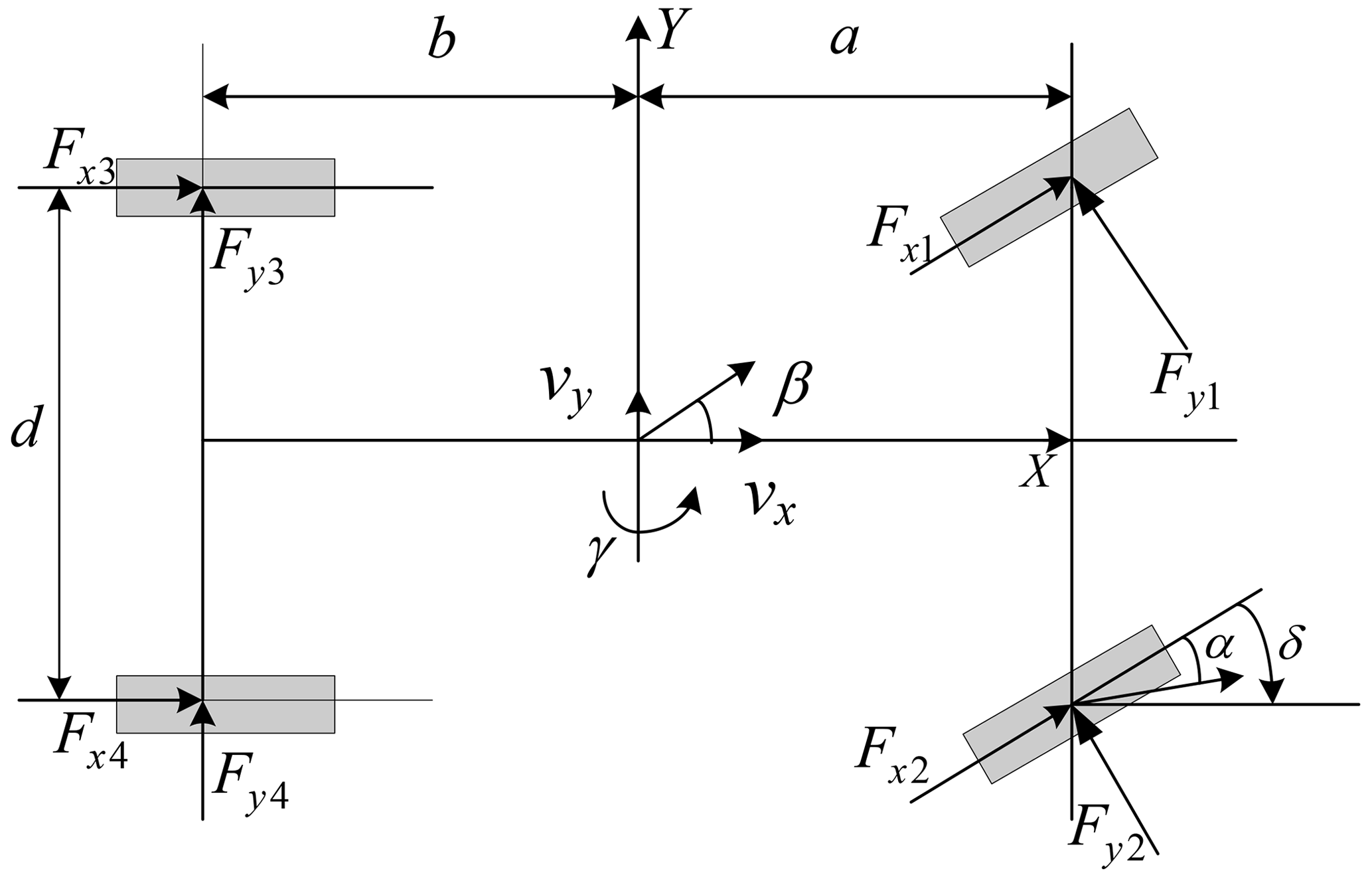
In this paper, the vehicle is simplified to a vehicle model with 7 degrees of freedom (Rajesh, 2012; Wang et al., 2017). The vehicle dynamics model is shown in Fig. 1, including the transverse motion, longitudinal motion, yaw motion and the rotational motion of four wheels around their respective axes.

The following assumptions are made with respect to the vehicle model:

1. the road surface is relatively smooth, although the movement and turning moment of the vehicle in the vertical direction are not considered;

2. the origin of the moving coordinate system solidified on the vehicle coincides with the center of mass of the vehicle;

3. each tire has the same mechanical characteristics;

4. the tire angle on the same shaft is the same in the steering process;

5. the pitch angle of the vehicle is zero, and the influence of the vehicle's roll motion on the motion is not considered.

The lateral motion is calculated as

$$\begin{array}{}\text{(1)}& \begin{array}{rl}m\left({\dot{v}}_y+v_{x}r\right)& =\left(F_{x\mathrm{1}}+F_{x\mathrm{2}}\right)\sin \mathit{\delta }\\ & +\left(F_{y\mathrm{1}}+F_{y\mathrm{2}}\right)\cos \mathit{\delta }+F_{y\mathrm{3}}+F_{y\mathrm{4}}\end{array}.\end{array}$$

The longitudinal motion is calculated as

$$\begin{array}{}\text{(2)}& \begin{array}{rl}m\left({\dot{v}}_x-v_{y}r\right)& =\left(F_{x\mathrm{1}}+F_{x\mathrm{2}}\right)\cos \mathit{\delta }\\ & -\left(F_{y\mathrm{1}}+F_{y\mathrm{2}}\right)\sin \mathit{\delta }+F_{x\mathrm{3}}+F_{x\mathrm{4}}.\end{array}\end{array}$$

The horizontal pendulum motion is calculated as

$$\begin{array}{}\text{(3)}& \begin{array}{rl}{I}_z\dot{r}& =a\left(F_{x\mathrm{1}}+F_{x\mathrm{2}}\right)\sin \mathit{\delta }-b\left(F_{y\mathrm{3}}+F_{y\mathrm{4}}\right)\\ & +a\left(F_{y\mathrm{1}}+F_{y\mathrm{2}}\right)\cos \mathit{\delta }+{\displaystyle \frac{d}{\mathrm{2}}}\left(F_{y\mathrm{1}}-F_{y\mathrm{2}}\right)\sin \mathit{\delta }\\ & +{\displaystyle \frac{d}{\mathrm{2}}}\left(F_{x\mathrm{2}}-F_{x\mathrm{1}}\right)\cos \mathit{\delta }.\end{array}\end{array}$$

The rolling motion of the wheels is calculated as

$$\begin{array}{}\text{(4)}& I_{\mathit{\omega }i}\dot{\mathit{\omega }}=T_{\mathrm{d}i}-F_{xi}{R}_{\mathrm{W}}-T_{\mathit{\mu }\mathrm{di}}\left(i=\mathrm{1},\mathrm{2},\mathrm{3},\mathrm{4}\right).\end{array}$$

In the above formulae, m is the mass of vehicle reconditioning (kg); v_x and v_y represent the velocities of vehicles in the x and y directions, respectively (m s⁻¹); r is vehicle yaw rate (rad s⁻¹); $F_{xi}\left(i=\mathrm{1},\mathrm{\dots },\mathrm{4}\right)$ and $F_{yi}\left(i=\mathrm{1},\mathrm{\dots },\mathrm{4}\right)$ represent the longitudinal force and transverse force of the tire, respectively, (N); $T_{\mathit{\mu }\mathrm{d}i}\left(i=\mathrm{1},\mathrm{\dots },\mathrm{4}\right)$ is dynamic output braking torque (N m); $T_{\mathrm{di}}\left(i=\mathrm{1},\mathrm{\dots },\mathrm{4}\right)$ is the wheel driving torque (N m); a and b represent the distance from the center of mass to the front and back axes, respectively (m); d is the wheel tread of both the front and rear wheels (m); δ is driver angle input (rad); I_z represents the rotational inertia which sprung mass around the z axis (kg m²); $I_{\mathrm{wi}}\left(i=\mathrm{1},\mathrm{\dots },\mathrm{4}\right)$ represents the rotational inertia of the wheels and their components (kg m²); R_w is wheel radius (m); and $w_i\left(i=\mathrm{1},\mathrm{\dots },\mathrm{4}\right)$ is the angular velocity of the wheel (rad s⁻¹).

2.2 Tire model

Considering the nonlinearity in the process of tire motion, the Dugoff model is adopted to analyze the force on the tire. In order to reflect the force on the actual road surface, an improved Dugoff tire model is used (Wu, 2008). For each wheel, the longitudinal force F_xi and lateral force F_yi can be expressed by the following formulae.

The longitudinal force of tire is calculated as

$$\begin{array}{}\text{(5)}& F_{xi}={\mathit{\mu }}_{xi}{F}_{zi}{C}_x{\displaystyle \frac{s}{\mathrm{1}+s}}f\left({\mathit{\lambda }}_i\right),\end{array}$$

where C_x is longitudinal slip stiffness, and λ_i is the set parameter.

The lateral force of tire is calculated as

$$\begin{array}{}\text{(6)}& F_{yi}={\mathit{\mu }}_{yi}{F}_{zi}{C}_y{\displaystyle \frac{\tan {\mathit{\alpha }}_i}{\mathrm{1}+s}}f\left({\mathit{\lambda }}_i\right);\end{array}$$

$$\begin{array}{}\text{(7)}& {\mathit{\lambda }}_i={\displaystyle \frac{\mathrm{1}-s}{\mathrm{2}\sqrt{{\left(C_{x}s\right)}^{\mathrm{2}}+{\left(C_y\tan \mathit{\alpha }\right)}^{\mathrm{2}}}}};\end{array}$$

$$\begin{array}{}\text{(8)}& f\left({\mathit{\lambda }}_i\right)=\left\{\begin{array}{l}\left(\mathrm{2}-{\mathit{\lambda }}_i\right){\mathit{\lambda }}_i\left({\mathit{\lambda }}_i\le \mathrm{1}\right)\\ \mathrm{1}\left({\mathit{\lambda }}_i>\mathrm{1}\right)\end{array}\right..\end{array}$$

Here, s represents the longitudinal slip of tire.

2.3 Vertical load of the wheel

The vertical load of each wheel is given as follows:

$$\begin{array}{}\text{(9)}& F_{z\mathrm{1}}={\displaystyle \frac{\mathrm{mgb}}{\mathrm{2}\left(a+b\right)}}-{\displaystyle \frac{{\mathrm{mh}}_{\mathrm{cg}}{\dot{v}}_x}{\mathrm{2}\left(a+b\right)}}-{\displaystyle \frac{{\mathrm{mh}}_{\mathrm{cg}}{\dot{v}}_{y}b}{\left(a+b\right)d}};\end{array}$$

$$\begin{array}{}\text{(10)}& F_{z\mathrm{2}}={\displaystyle \frac{\mathrm{mgb}}{\mathrm{2}\left(a+b\right)}}-{\displaystyle \frac{{\mathrm{mh}}_{\mathrm{cg}}{\dot{v}}_x}{\mathrm{2}\left(a+b\right)}}+{\displaystyle \frac{{\mathrm{mh}}_{\mathrm{cg}}{\dot{v}}_{y}b}{\left(a+b\right)d}};\end{array}$$

$$\begin{array}{}\text{(11)}& F_{z\mathrm{3}}={\displaystyle \frac{\mathrm{mga}}{\mathrm{2}\left(a+b\right)}}+{\displaystyle \frac{{\mathrm{mh}}_{\mathrm{cg}}{\dot{v}}_x}{\mathrm{2}\left(a+b\right)}}-{\displaystyle \frac{{\mathrm{mh}}_{\mathrm{cg}}{\dot{v}}_{y}a}{\left(a+b\right)d}};\end{array}$$

$$\begin{array}{}\text{(12)}& F_{z\mathrm{4}}={\displaystyle \frac{\mathrm{mga}}{\mathrm{2}\left(a+b\right)}}+{\displaystyle \frac{{\mathrm{mh}}_{\mathrm{cg}}{\dot{v}}_x}{\mathrm{2}\left(a+b\right)}}+{\displaystyle \frac{{\mathrm{mh}}_{\mathrm{cg}}{\dot{v}}_{y}a}{\left(a+b\right)d}}.\end{array}$$

2.4 Each wheel side-slip angle and the speed of the wheel center

The angle of each wheel side-slip and the speed of the wheel center are given as follows:

$$\begin{array}{}\text{(13)}& {\mathit{\alpha }}_{\mathrm{1}}={\tan }^{-\mathrm{1}}\left({\displaystyle \frac{v_y+a\mathit{\gamma }}{v_y-\mathrm{0.5}d\mathit{\gamma }}}\right)-{\mathit{\delta }}_f;\end{array}$$

$$\begin{array}{}\text{(14)}& {\mathit{\alpha }}_{\mathrm{2}}={\tan }^{-\mathrm{1}}\left({\displaystyle \frac{v_y+a\mathit{\gamma }}{v_y+\mathrm{0.5}d\mathit{\gamma }}}\right)-{\mathit{\delta }}_f;\end{array}$$

$$\begin{array}{}\text{(15)}& {\mathit{\alpha }}_{\mathrm{3}}={\tan }^{-\mathrm{1}}\left({\displaystyle \frac{v_y-b\mathit{\gamma }}{v_x-\mathrm{0.5}d\mathit{\gamma }}}\right);\end{array}$$

$$\begin{array}{}\text{(16)}& {\mathit{\alpha }}_{\mathrm{4}}={\tan }^{-\mathrm{1}}\left({\displaystyle \frac{v_y-b\mathit{\gamma }}{v_x+\mathrm{0.5}d\mathit{\gamma }}}\right);\end{array}$$

$$\begin{array}{}\text{(17)}& v_{x\mathrm{1}}=\left(v_x-\mathrm{0.5}dr\right)\cos \mathit{\delta }+\left(v_y+\mathrm{ar}\right)\sin \mathit{\delta };\end{array}$$

$$\begin{array}{}\text{(18)}& v_{x\mathrm{2}}=\left(v_x+\mathrm{0.5}dr\right)\cos \mathit{\delta }+\left(v_y+\mathrm{ar}\right)\sin \mathit{\delta };\end{array}$$

$$\begin{array}{}\text{(19)}& v_{x\mathrm{3}}=\left(v_x-\mathrm{0.5}dr\right);\end{array}$$

$$\begin{array}{}\text{(20)}& v_{x\mathrm{4}}=\left(v_x+\mathrm{0.5}dr\right).\end{array}$$

2.5 Slip rate calculation

The slip rate is calculated as

$$\begin{array}{}\text{(21)}& s={\displaystyle \frac{v-v_i}{v}}\times \mathrm{100}\mathit{\%}=\left(\mathrm{1}-{\displaystyle \frac{{\mathit{\omega }}_i{R}_{\mathrm{w}}}{v}}\right)\times \mathrm{100}\mathit{\%}\left(i=\mathrm{1},\mathrm{2},\mathrm{3},\mathrm{4}\right),\end{array}$$

where R_w is the radius of the wheel, ${\mathit{\omega }}_i\left(i=\mathrm{1},\mathrm{\cdots },\mathrm{4}\right)$ is the angular velocity of the wheel and $v_{xi}\left(i=\mathrm{1},\mathrm{\cdots },\mathrm{4}\right)$ is the velocity of the wheel center.

3 Estimation of the road adhesion coefficient based on the UKF algorithm

The extended Kalman filter algorithm is used to carry out Taylor expansion of the nonlinear system equations or observation equations and keep the first-order approximation term, so that the linearization error will be introduced. In general, the extended Kalman filter needs to calculate the Jacobian matrix of the system state equations and observation equations, which increases the complexity of the calculation. Compared with the extended Kalman filter, the UKF discards the traditional method of linearizing the nonlinear function, uses the unscented transform (UT) change to determine the sampling point near the estimated point and uses the determined sample to approximate the posterior probability density of the state. It does not need to derivative the Jacobian matrix, and it improves the estimation accuracy and stability (Huang and Wang, 2015).

Assuming that the process noise and the observation noise are both Gaussian white noise and that the variances are Q and R, respectively, the nonlinear system is described as follows:

$$\begin{array}{}\text{(22)}& \left\{\begin{array}{l}X(k+\mathrm{1})=f\left(X\right(k),W(k\left)\right)\\ Z\left(k\right)=h\left(X\right(k),V(k\left)\right),\end{array}\right.\end{array}$$

where W(k) is the process noise, V(k) is the observation noise, f is the nonlinear state equation function and h is the nonlinear observation equation function. The basic steps in the calculation are as follows:

1. Calculate the weights corresponding to 2n+1 sigma points and sampling points.

   $$\begin{array}{}\text{(23)}& \left\{\begin{array}{l}{X}^{\left(\mathrm{0}\right)}=\stackrel{\mathrm{‾}}{X},i=\mathrm{0}\\ X^{\left(i\right)}=\stackrel{\mathrm{‾}}{X}+(\sqrt{(n+\mathit{\lambda })P}{)}_i,i=\mathrm{1}-n\\ X^{\left(i\right)}=\stackrel{\mathrm{‾}}{X}-(\sqrt{(n+\mathit{\lambda })P}{)}_i,i=n+\mathrm{1}-\mathrm{2}n\end{array}\right.\end{array}$$
   $$\begin{array}{}\text{(24)}& \left\{\begin{array}{l}{\mathit{\omega }}_{\mathrm{m}}^{\mathrm{0}}=\frac{\mathit{\lambda }}{n+\mathit{\lambda }}\\ {\mathit{\omega }}_{\mathrm{c}}^{\mathrm{0}}=\frac{\mathit{\lambda }}{n+\mathit{\lambda }}+(\mathrm{1}-a_t^{\mathrm{2}}+\mathit{\beta })\\ {\mathit{\omega }}_{\mathrm{m}}^i={\mathit{\omega }}_{\mathrm{c}}^i=\frac{\mathit{\lambda }}{\mathrm{2}(n+\mathit{\lambda })},i=\mathrm{1}-\mathrm{2}n,\end{array}\right.\end{array}$$

   where

   $$\begin{array}{}\text{(25)}& \mathit{\lambda }=a_t^{\mathrm{2}}(n+\mathit{\kappa })-n.\end{array}$$

   In the formula $\left(\sqrt{\mathbf{P}}{)}^T\right(\sqrt{\mathbf{P}})=\mathbf{P}$, $(\sqrt{\mathbf{P}}{)}_i$ represents the ith column of the square root of the matrix; ω_c is the weight of the covariance; ω_m is the weight of the mean; λ is the scaling factor to reduce the prediction error; a_t is the distribution state of sampling point; κ is a parameter to be selected, and its value should ensure that matrix (n+λ)P is a positive semi-definite matrix; and β is the parameter to be selected, and its value is β≥0, which is used to combine the momentum of the higher-order terms in the equation.

2. A set of sampling points and their weights are obtained using Eqs. (23) and (24).

   $$\begin{array}{}\text{(26)}& \begin{array}{c}{X}^{\left(i\right)}\left(k\mathrm{|}k\right)=\begin{array}{cc}\left[\widehat{X}\left(k\mathrm{|}k\right)\right.& \widehat{X}\left(k\mathrm{|}k\right)+\sqrt{\left(n+\mathit{\lambda }\right)P\left(k\mathrm{|}k\right)}\end{array}\\ \left.\widehat{X}\left(k\mathrm{|}k\right)-\sqrt{\left(n+\mathit{\lambda }\right)P\left(k\mathrm{|}k\right)}\right]\end{array}\end{array}$$

3. Calculate the further prediction of the 2n+1 sigma point set, $i=\mathrm{1},\mathrm{2},\mathrm{\cdots },\mathrm{2}n+\mathrm{1}$, using

   $$\begin{array}{}\text{(27)}& X^{\left(i\right)}(k+\mathrm{1}\mathrm{|}k)=f[k,X^{\left(i\right)}(k\mathrm{|}k\left)\right].\end{array}$$

4. According to the sigma point, calculate the further prediction of the system state quantity and the covariance matrix as

   $$\begin{array}{}\text{(28)}& \widehat{X}\left(k+\mathrm{1}\mathrm{|}k\right)=\sum _{i=\mathrm{0}}^{\mathrm{2}n}{\mathit{\omega }}^{\left(i\right)}{X}^{\left(i\right)}\left(k+\mathrm{1}\mathrm{|}k\right);\end{array}$$
   $$\begin{array}{}\text{(29)}& \begin{array}{rl}P\left(k+\mathrm{1}\mathrm{|}k\right)& =\sum _{i=\mathrm{0}}^{\mathrm{2}n}{\mathit{\omega }}^{\left(i\right)}\left[\widehat{X}\left(k+\mathrm{1}\mathrm{|}k\right)-X^{\left(i\right)}\left(k+\mathrm{1}\mathrm{|}k\right)\right]\\ & \cdot \left[\widehat{X}\left(k+\mathrm{1}\mathrm{|}k\right)-X^{\left(i\right)}\left(k+\mathrm{1}\mathrm{|}k\right)\right]+Q.\end{array}\end{array}$$

5. According to the predicted value, the UT transformation is used again to generate a new sigma point set, and the generated new sigma point set is substituted into the observation equation to obtain the predicted observation value.

   $$\begin{array}{}\text{(30)}& \begin{array}{c}{X}^{\left(i\right)}\left(k+\mathrm{1}\mathrm{|}k\right)=\begin{array}{cc}\left[\widehat{X}\left(k+\mathrm{1}\mathrm{|}k\right)\right.& \widehat{X}\left(k+\mathrm{1}\mathrm{|}k\right)+\sqrt{\left(n+\mathit{\lambda }\right)P\left(k+\mathrm{1}\mathrm{|}k\right)}\end{array}\\ \left.\widehat{X}\left(k+\mathrm{1}\mathrm{|}k\right)-\sqrt{\left(n+\mathit{\lambda }\right)P\left(k+\mathrm{1}\mathrm{|}k\right)}\right]\end{array}\end{array}$$
   $$\begin{array}{}\text{(31)}& Z^{\left(i\right)}\left(k+\mathrm{1}\mathrm{|}k\right)=h\left[X^{\left(i\right)}\left(k+\mathrm{1}\mathrm{|}k\right)\right]\end{array}$$

6. Obtain the observed prediction value of the sigma point set from the above steps, and obtain the mean value and covariance of the system prediction via weighted summation.

   $$\begin{array}{}\text{(32)}& \stackrel{\mathrm{‾}}{Z}\left(k+\mathrm{1}\mathrm{|}k\right)=\sum _{i=\mathrm{0}}^{\mathrm{2}n}{\mathit{\omega }}^{\left(i\right)}{Z}^{\left(i\right)}\left(k+\mathrm{1}\mathrm{|}k\right)\end{array}$$
   $$\begin{array}{}\text{(33)}& \begin{array}{rl}{P}_{Z_k{Z}_k}& =\sum _{i=\mathrm{0}}^{\mathrm{2}n}{\mathit{\omega }}^{\left(i\right)}\left[Z^{\left(i\right)}\left(k+\mathrm{1}\mathrm{|}k\right)-\stackrel{\mathrm{‾}}{Z}\left(k+\mathrm{1}\mathrm{|}k\right)\right]\\ & \cdot \left[Z^{\left(i\right)}\left(k+\mathrm{1}\mathrm{|}k\right)-\stackrel{\mathrm{‾}}{Z}\left(k+\mathrm{1}\mathrm{|}k\right)\right]+R\end{array}\end{array}$$
   $$\begin{array}{}\text{(34)}& \begin{array}{rl}{P}_{X_k{Z}_k}& =\sum _{i=\mathrm{0}}^{\mathrm{2}n}{\mathit{\omega }}^{\left(i\right)}\left[X^{\left(i\right)}\left(k+\mathrm{1}\mathrm{|}k\right)\right.\\ & \left.-\stackrel{\mathrm{‾}}{Z}\left(k+\mathrm{1}\mathrm{|}k\right)\right]{\left[X^{\left(i\right)}\left(k+\mathrm{1}\mathrm{|}k\right)-\stackrel{\mathrm{‾}}{Z}\left(k+\mathrm{1}\mathrm{|}k\right)\right]}^T\end{array}\end{array}$$

7. Calculate the Kalman gain matrix.

   $$\begin{array}{}\text{(35)}& K\left(k+\mathrm{1}\right)=P_{X_k{Z}_k}{P}_{Z_k{Z}_k}^{-\mathrm{1}}\end{array}$$

8. Calculate the status update and covariance update of the system.

   $$\begin{array}{}\text{(36)}& \begin{array}{rl}\widehat{X}\left(k+\mathrm{1}\mathrm{|}k+\mathrm{1}\right)& =\widehat{X}\left(k+\mathrm{1}\mathrm{|}k\right)+K\left(k+\mathrm{1}\right)\left[Z\left(k+\mathrm{1}\mathrm{|}\right)\right.\\ & \left.-\widehat{Z}\left(k+\mathrm{1}\mathrm{|}k\right)\right]\end{array}\end{array}$$
   $$\begin{array}{}\text{(37)}& \begin{array}{rl}P\left(k+\mathrm{1}\mathrm{|}k+\mathrm{1}\right)& =P\left(k+\mathrm{1}\mathrm{|}k\right)\\ & -K\left(k+\mathrm{1}\right)P_{Z_k{Z}_k}{K}^T\left(k+\mathrm{1}\right)\end{array}\end{array}$$

In order to estimate the road adhesion coefficient, the state variable of the nonlinear automobile system is set to $\mathbf{X}=[{\mathit{\mu }}_{\mathrm{1}},{\mathit{\mu }}_{\mathrm{2}},{\mathit{\mu }}_{\mathrm{3}},{\mathit{\mu }}_{\mathrm{4}}{]}^T$, and the observed variable is $\mathbf{Z}=[a_x,a_y,\dot{r}{]}^T$.

Combined with the above vehicle dynamics model, the vehicle nonlinear system can be described as

$$\begin{array}{}\text{(38)}& X(k+\mathrm{1})=\left[\begin{array}{cccc}\mathrm{1}& \mathrm{0}& \mathrm{0}& \mathrm{0}\\ \mathrm{0}& \mathrm{1}& \mathrm{0}& \mathrm{0}\\ \mathrm{0}& \mathrm{0}& \mathrm{1}& \mathrm{0}\\ \mathrm{0}& \mathrm{0}& \mathrm{0}& \mathrm{1}\end{array}\right]\left[\begin{array}{c}{\mathit{\mu }}_{\mathrm{1}}\\ {\mathit{\mu }}_{\mathrm{2}}\\ {\mathit{\mu }}_{\mathrm{3}}\\ {\mathit{\mu }}_{\mathrm{4}}\end{array}\right]+W\left(k\right);\end{array}$$

$$\begin{array}{}\text{(39)}& Z\left(k\right)=\mathit{\varphi }X\left(k\right)+V\left(k\right).\end{array}$$

Here,

$$\begin{array}{}\text{(40)}& \mathit{\varphi }=\left[\begin{array}{cccc}\frac{F_{x\mathit{\_}fl}^{\mathrm{0}}-F_{y\mathit{\_}fl}^{\mathrm{0}}\mathit{\delta }}{m}& \frac{F_{x\mathit{\_}fr}^{\mathrm{0}}-F_{y\mathit{\_}fr}^{\mathrm{0}}\mathit{\delta }}{m}& \frac{F_{x\mathit{\_}rl}^{\mathrm{0}}}{m}& \frac{F_{x\mathit{\_}rr}^{\mathrm{0}}}{m}\\ \frac{F_{x\mathit{\_}fl}^{\mathrm{0}}\mathit{\delta }+F_{y\mathit{\_}fl}^{\mathrm{0}}}{m}& \frac{F_{x\mathit{\_}fr}^{\mathrm{0}}\mathit{\delta }+F_{y\mathit{\_}fr}^{\mathrm{0}}}{m}& \frac{F_{y\mathit{\_}rl}^{\mathrm{0}}}{m}& \frac{F_{y\mathit{\_}rr}^{\mathrm{0}}}{m}\\ H(\mathrm{3},\mathrm{1})& H(\mathrm{3},\mathrm{2})& H(\mathrm{3},\mathrm{3})& H(\mathrm{3},\mathrm{4})\end{array}\right];\end{array}$$

$$\begin{array}{l}H\left(\mathrm{3},\mathrm{1}\right)=\frac{a\left(F_{x\mathit{\_}fl}^{\mathrm{0}}\mathit{\delta }+F_{y\mathit{\_}fl}^{\mathrm{0}}\right)+d/\phantom{d\mathrm{2}}\mathrm{2}\left(F_{x\mathit{\_}fl}^{\mathrm{0}}-F_{y\mathit{\_}fl}^{\mathrm{0}}\mathit{\delta }\right)}{I_z};\\ H\left(\mathrm{3},\mathrm{2}\right)=\frac{a\left(F_{x\mathit{\_}fr}^{\mathrm{0}}\mathit{\delta }+F_{y\mathit{\_}fr}^{\mathrm{0}}\right)-d/\phantom{d\mathrm{2}}\mathrm{2}\left(F_{x\mathit{\_}fr}^{\mathrm{0}}-F_{y\mathit{\_}fr}^{\mathrm{0}}\mathit{\delta }\right)}{I_z};\\ H\left(\mathrm{3},\mathrm{3}\right)=\frac{-\left(b{F}_{y\mathit{\_}rl}^{\mathrm{0}}-d/\phantom{d\mathrm{2}}\mathrm{2}{F}_{x\mathit{\_}rl}^{\mathrm{0}}\right)}{I_z};\\ H\left(\mathrm{3},\mathrm{4}\right)=\frac{-\left(b{F}_{y\mathit{\_}rr}^{\mathrm{0}}+d/\phantom{d\mathrm{2}}\mathrm{2}{F}_{x\mathit{\_}rr}^{\mathrm{0}}\right)}{I_z}.\end{array}$$

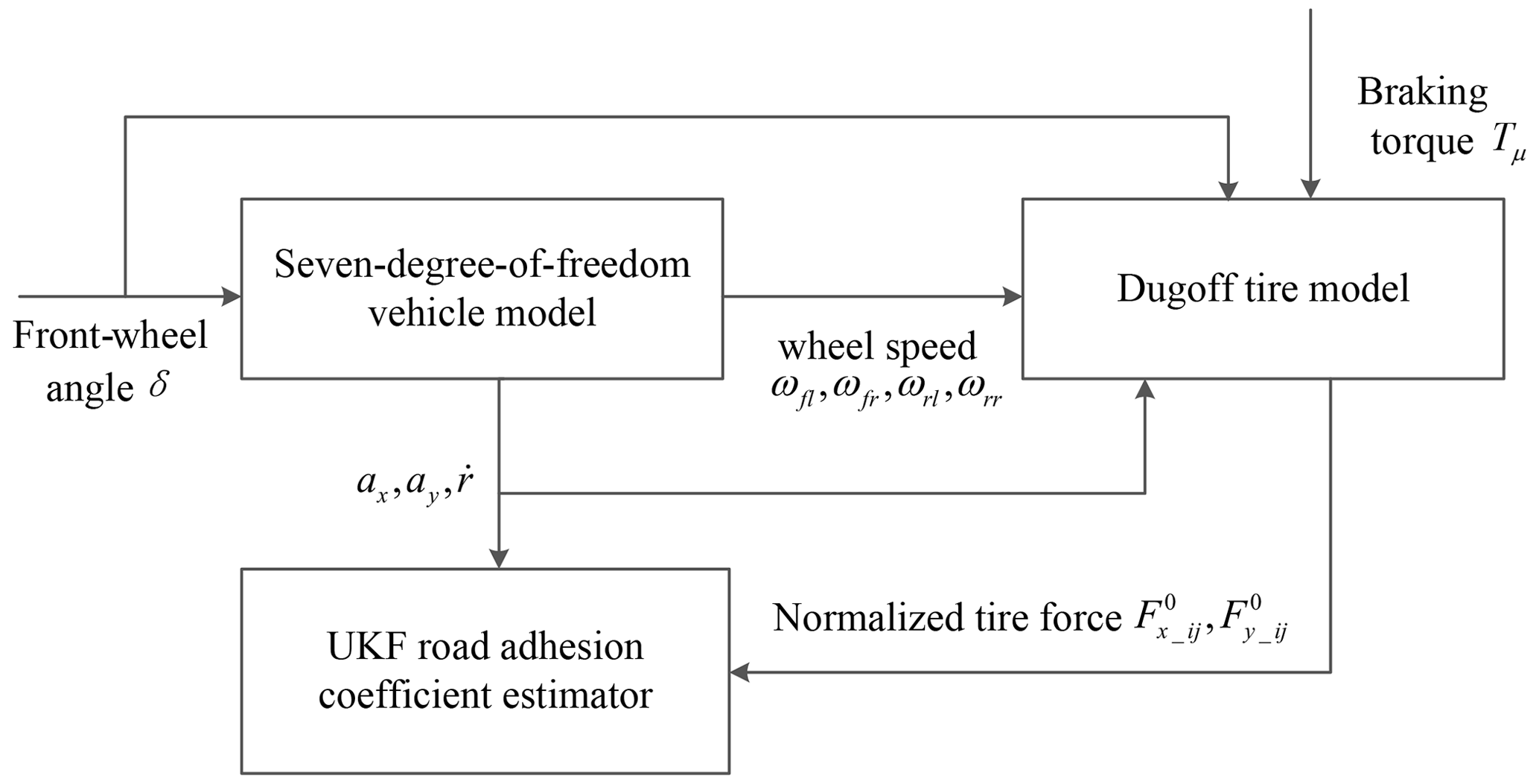
In combination with the actual operating conditions of the vehicle, the initial value of the filter is set as follows: the process noise covariance matrix is $\mathbf{R}=I_{\mathrm{3}\cdot \mathrm{3}}$, the measurement noise covariance matrix is $\mathbf{Q}=I_{\mathrm{4}\cdot \mathrm{4}}\cdot \mathrm{0.01}$, and the initial value of the error covariance matrix is ${\mathbf{P}}_{\mathrm{0}}=I_{\mathrm{4}\cdot \mathrm{4}}$. After the initial value setting is completed, the algorithm recursion is realized. The vehicle model and the Dugoff normalized tire model are built in MATLAB–Simulink, and the road adhesion coefficient is the estimated by filtering with the UKF. The schematic diagram of road adhesion coefficient estimation based on the UKF algorithm is shown in Fig. 2.

Table 1 Vehicle structure parameters.

4 Estimation of the road adhesion coefficient based on the PF algorithm

For the parameter estimation of a nonlinear vehicle system, in addition to the KF algorithm mentioned above, another possible method for use is the PF algorithm. The core idea of the PF algorithm is the approximation of the probability density function of the system state variables using a series of discrete sampling points. The minimum variance of the state variables is obtained by using the sample mean value, and the estimated value of the system state is then obtained (Huang and Wang, 2017). The algorithm is not limited by noise type nor system type, and it has great advantages with respect to dealing with nonlinear and non-Gaussian systems. The PF algorithm is a probabilistic statistical method, comprising a Bayesian filtering algorithm based on Monte Carlo simulation. It estimates the identified parameters by calculating the mean value of the particle set samples.

Figure 5 The high-adhesion road surface identification effect based on the UKF algorithm.

Figure 6 The high-adhesion road surface identification effect based on the PF algorithm.

Figure 7 The low-adhesion road surface identification effect based on the UKF algorithm.

Figure 8 The low-adhesion road surface identification effect based on the PF algorithm.

Figure 9 The hub-motor experimental car.

Table 2 Vehicle structure parameters.

Figure 10 Driving route map.

Figure 11 Lateral acceleration.

Figure 12 Yaw rate.

Figure 13 Longitudinal acceleration.

The PF algorithm used in the process of estimating the road adhesion coefficient in this paper is a classic sampling importance resampling (SIR) algorithm. This algorithm introduces resampling, which can effectively avoid the particle degradation problem by moving the particles to the high likelihood region as much as possible. In the process of estimating the road adhesion coefficient, a small number of particles are used, and good results can be obtained, which improves the real-time performance of parameter estimation (Lin et al., 2011). The specific process of the algorithm is described below.

For a nonlinear system, the process of the algorithm is described as follows:

$$\begin{array}{}\text{(41)}& X\left(k\right)=f\left(X\left(k-\mathrm{1}\right),W\left(k\right)\right);\end{array}$$

$$\begin{array}{}\text{(42)}& Z\left(k\right)=h\left(X\left(k\right),V\left(k\right)\right).\end{array}$$

Here, X(k) is the state variable at time k; Z(k) is the measured variable at time k; W(k) is the process noise, and its variance is Q; and V(k) is the observation noise, and its variance is R.

The steps required to implement the filter are as follows:

1. Initialize the filter.

   N random samples are drawn from the prior distribution p(X₀), and the particle swarm $\mathit{\{}{X}_{\mathrm{0}:k}^i{\mathit{\}}}_{i=\mathrm{1}}^N$ is generated. The weights are normalized to $\sum _i{\mathit{\omega }}_k^i=\mathrm{1}$, and the weights of all particles are set to $\mathrm{1}/N$. The posterior probability distribution of the target state at time k can then be discretely weighted as

   $$\begin{array}{}\text{(43)}& p\left(X_{\mathrm{0}:k}\mathrm{|}{Z}_{\mathrm{1}:k}\right)\approx \sum _{i=\mathrm{1}}^N{\mathit{\omega }}_k^i\mathit{\delta }\left(X_{\mathrm{0}:k}-X_{\mathrm{0}:k}^i\right),\end{array}$$

   where X_0:k is the state set from 0 to k, $X_{\mathrm{0}:k}^i$ is the particle set with corresponding weight ${\mathit{\omega }}_k^i$, δ(X) is the Dirac-delta function and Z_1:k is the measured value.

   The posterior probability density is updated with the update of the observation. The initial error variance matrix is set as a fourth-order sparse matrix with diagonal elements of 10⁻³. Among them, the variance setting is small, which can avoid generating excessive disturbance and causing distortion.

2. Calculate the of importance weights.

   The choice of weight is the key to particle filtering. The weight is selected by importance sampling. Sampling $X_k^{\left(i\right)}\sim q(X_k\mathrm{|}{X}_{\mathrm{0}:k-\mathrm{1}},Z_{\mathrm{1}:k})$, the update formula of importance weight is

   $$\begin{array}{}\text{(44)}& \begin{array}{rl}& {\mathit{\omega }}_k^i\propto {\displaystyle \frac{p\left(Z_k\mathrm{|}{X}_k^i\right)p\left(X_k^i\mathrm{|}{X}_{k-\mathrm{1}}^i\right)p\left(X_{\mathrm{0}:k-\mathrm{1}}^i\mathrm{|}{Z}_{\mathrm{1}:k-\mathrm{1}}\right)}{q\left(X_k^i\mathrm{|}{X}_{\mathrm{0}:k-\mathrm{1}}^i,Z_{\mathrm{1}:k}\right)q\left(X_{\mathrm{0}:k-\mathrm{1}}^i\mathrm{|}{Z}_{\mathrm{1}:k-\mathrm{1}}\right)}}=\\ & {\mathit{\omega }}_{k-\mathrm{1}}^i{\displaystyle \frac{p\left(Z_k\mathrm{|}{X}_k^i\right)p\left(X_k^i\mathrm{|}{X}_{k-\mathrm{1}}^i\right)}{q\left(X_k^i\mathrm{|}{X}_{\mathrm{0}:k-\mathrm{1}}^i,Z_{\mathrm{1}:k}\right)}}.\end{array}\end{array}$$

   The importance weight is then normalized as

   $$\begin{array}{}\text{(45)}& {\mathit{\omega }}_k^i={\mathit{\omega }}_k^i/\phantom{{\mathit{\omega }}_k^i\sum _{i=\mathrm{1}}^N{\mathit{\omega }}_k^i}\sum _{i=\mathrm{1}}^N{\mathit{\omega }}_k^i.\end{array}$$

3. Introduce resampling.

   To overcome the problem of particle degradation, resampling technology is introduced. The degradation problem of particle filtering algorithm is that the variance of the importance weight increases randomly with time, so that the weight of particles is concentrated on a few particles. Even after several steps of recursion, there may be only one particle with nonzero weight. The weight of other particles is small, which can be ignored, so that a great deal of computational work is wasted updating particles that have little or no effect on the estimate of p(X_k|Z_1:k); as a result, the set of particles cannot represent the actual posterior probability distribution. In order to determine the degradation degree of particles, an approximate measurement scale of relative efficiency is adopted. This effective sampling scale N_eff is defined as outlined in Zhu (2010),

   $$\begin{array}{}\text{(46)}& N_{\mathrm{eff}}=\mathrm{1}/\phantom{\mathrm{1}\sum _{i=\mathrm{1}}^N({\mathit{\omega }}_k^i{)}^{\mathrm{2}}}\sum _{i=\mathrm{1}}^N({\mathit{\omega }}_k^i{)}^{\mathrm{2}}.\end{array}$$

   An effective sample number N_threshold is then set as the threshold. When N_eff<N_threshold, resampling is performed, and the original weighted sample $\mathit{\{}{X}_{\mathrm{0}:k}^i,{\mathit{\omega }}_k^i{\mathit{\}}}_{i=\mathrm{1}}^N$ is mapped to $\mathit{\{}{X}_{\mathrm{0}:k}^i,N^{-\mathrm{1}}{\mathit{\}}}_{i=\mathrm{1}}^N$ equal weighted samples.

4. Obtain output.

   The state estimation as carried out as

   $$\begin{array}{}\text{(47)}& X_k=\sum _{i=\mathrm{1}}^N{\mathit{\omega }}_k^i{X}_k^i.\end{array}$$

   The variance estimation is calculated as

   $$\begin{array}{}\text{(48)}& P_k=\sum _{i=\mathrm{1}}^N{\mathit{\omega }}_k^i\left(X_k^i-X_k\right){\left(X_k^i-X_k\right)}^T.\end{array}$$

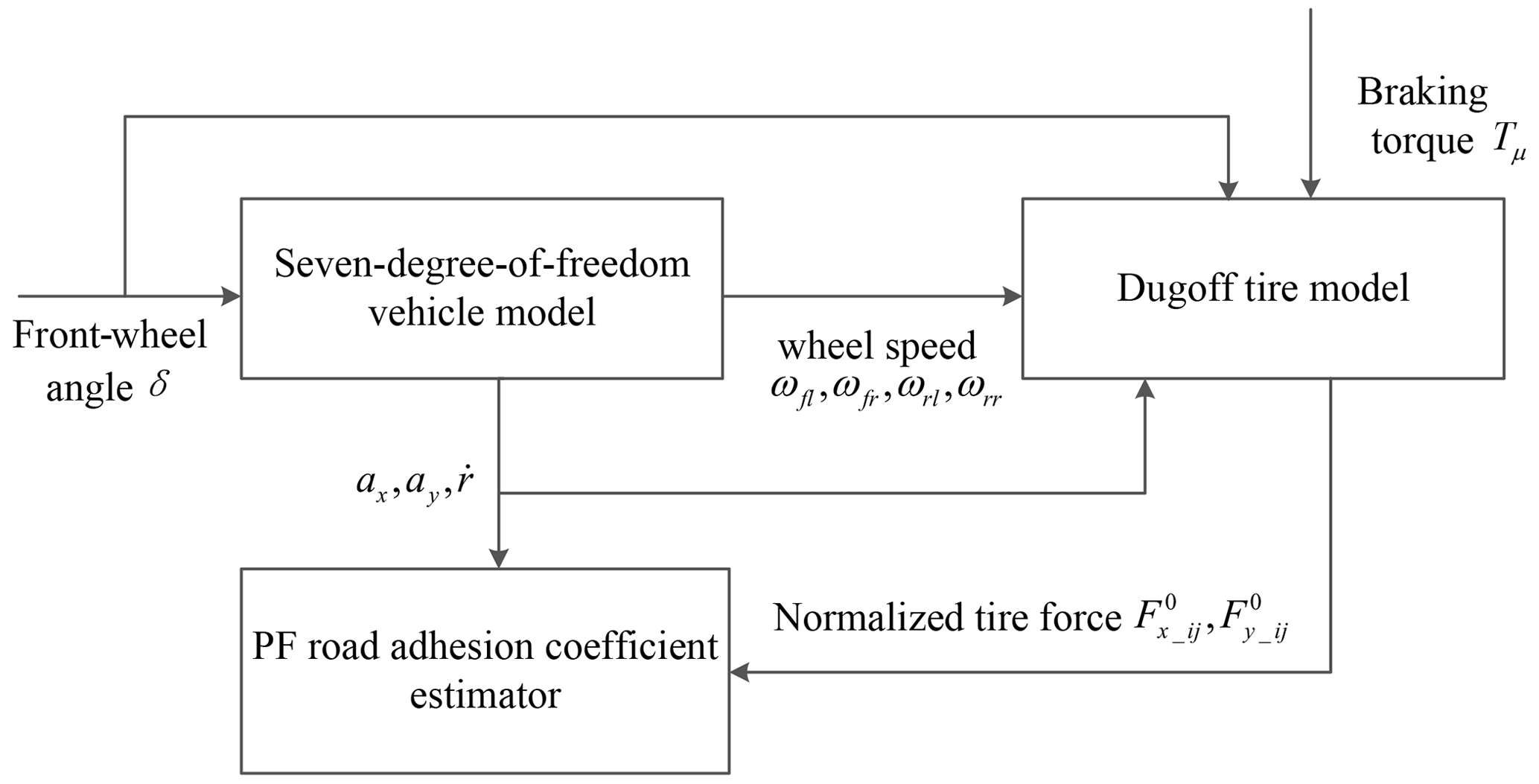
   The vehicle model and the Dugoff normalized tire model are built in MATLAB–Simulink, and the road adhesion coefficient is finally estimated by filtering with the PF. A schematic diagram of the road adhesion coefficient estimation based on the PF algorithm is shown in Fig. 3.

Figure 14 Front-wheel angle.

Figure 15 Road surface identification effect of double-lane-changing conditions.

5 Results & discussion

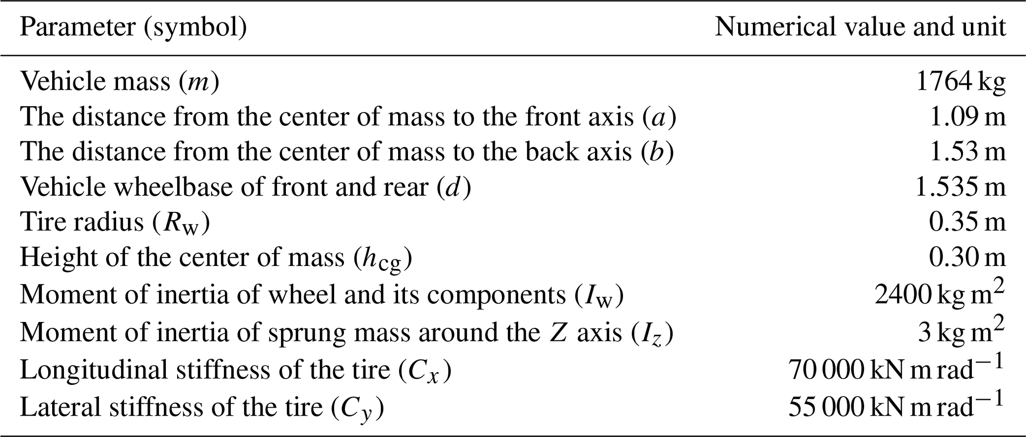
Taking the four-wheel motor drive prototype developed by our research group as the research object, road adhesion coefficient estimators are studied. The vehicle structure parameters are shown in Table 1.

The simulation experiment is carried out under the double-lane-changing conditions outlined below, and the front-wheel angle of the double-lane-changing test is shown in Fig. 4. The abovementioned vehicle model and the designed algorithm observer are used to estimate the road adhesion coefficient.

5.1 Simulation of road adhesion coefficient estimation

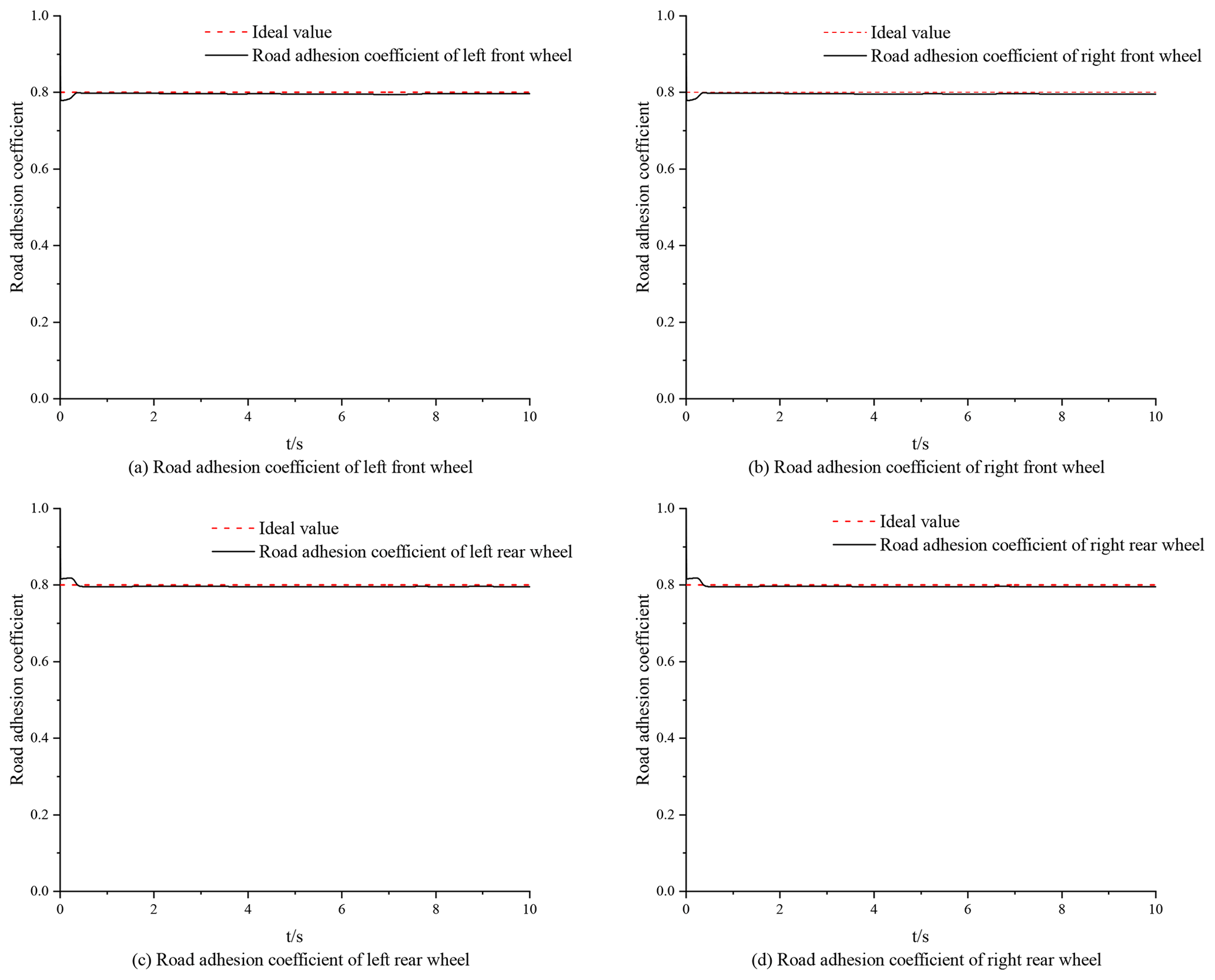
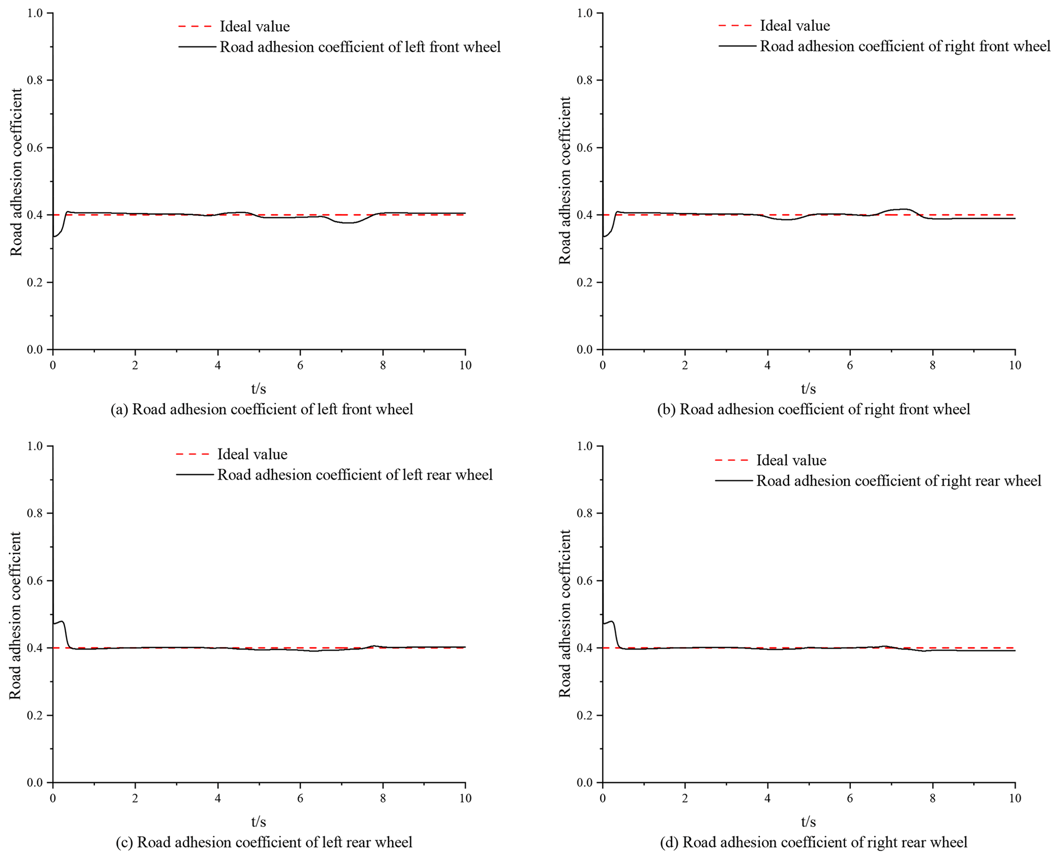
An established 7-DOF vehicle model and the Dugoff tire model are used to identify the road adhesion coefficient according to the designed UKF algorithm and PF algorithm. In order to verify the effectiveness and feasibility of the algorithms with respect to identifying the road adhesion coefficient, according to the built Simulink simulation model, the simulation tests are carried out on roads with high and low adhesion coefficients. The simulation tests' conditions were the abovementioned double-lane-changing conditions, the vehicle speed was 48 km h⁻¹, and the ideal high and low adhesion coefficients were set to 0.8 and 0.4, respectively.

The initial value settings of the road adhesion coefficient estimator based on the UKF algorithm were as follows: the process noise covariance matrix was $\mathbf{R}=I_{\mathrm{3}\cdot \mathrm{3}}$, the measured noise covariance matrix was $\mathbf{Q}=I_{\mathrm{4}\cdot \mathrm{4}}\cdot \mathrm{0.01}$, the initial value ${\mathbf{P}}_{\mathrm{0}}=I_{\mathrm{4}\cdot \mathrm{4}}$ of the error covariance matrix and the initial value of the state variable was $\mathbf{X}=[\mathrm{1},\mathrm{1},\mathrm{1},\mathrm{1}]$

The initial value settings of the road adhesion coefficient estimator based on the PF algorithm were as follows: the process noise covariance matrix was R=[1], the measured noise covariance matrix was $\mathbf{Q}=I_{\mathrm{4}\cdot \mathrm{4}}\cdot \mathrm{0.01}$, the initial value ${\mathbf{P}}_{\mathrm{0}}=I_{\mathrm{4}\cdot \mathrm{4}}$ of the error covariance matrix and the initial value of the state variable was $\mathbf{X}=[\mathrm{1},\mathrm{1},\mathrm{1},\mathrm{1}]$.

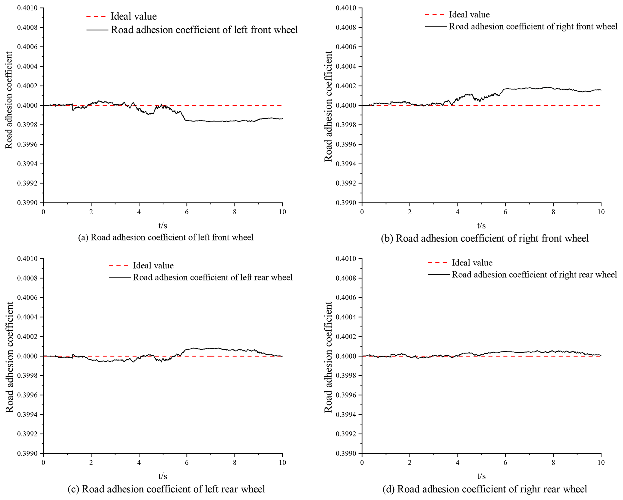
According to the simulation results on high- and low-adhesion-coefficient roads, both the UKF algorithm and the PF algorithm can effectively estimate the road adhesion coefficient in real time, showing good robustness. According to Figs. 5–8, the time for the UKF algorithm to converge to the ideal value is significantly longer than for the PF algorithm, but the convergence time is also within 1 s. Via comparison and analysis, the estimation of the road adhesion coefficient based on the PF algorithm is closer to the ideal value. Both algorithms will oscillate due to the measurement noise, resulting in errors. Compared with the UKF algorithm, the estimation of the road adhesion coefficient based on the PF algorithm has a higher accuracy and better control effect.

5.2 Experimental verification

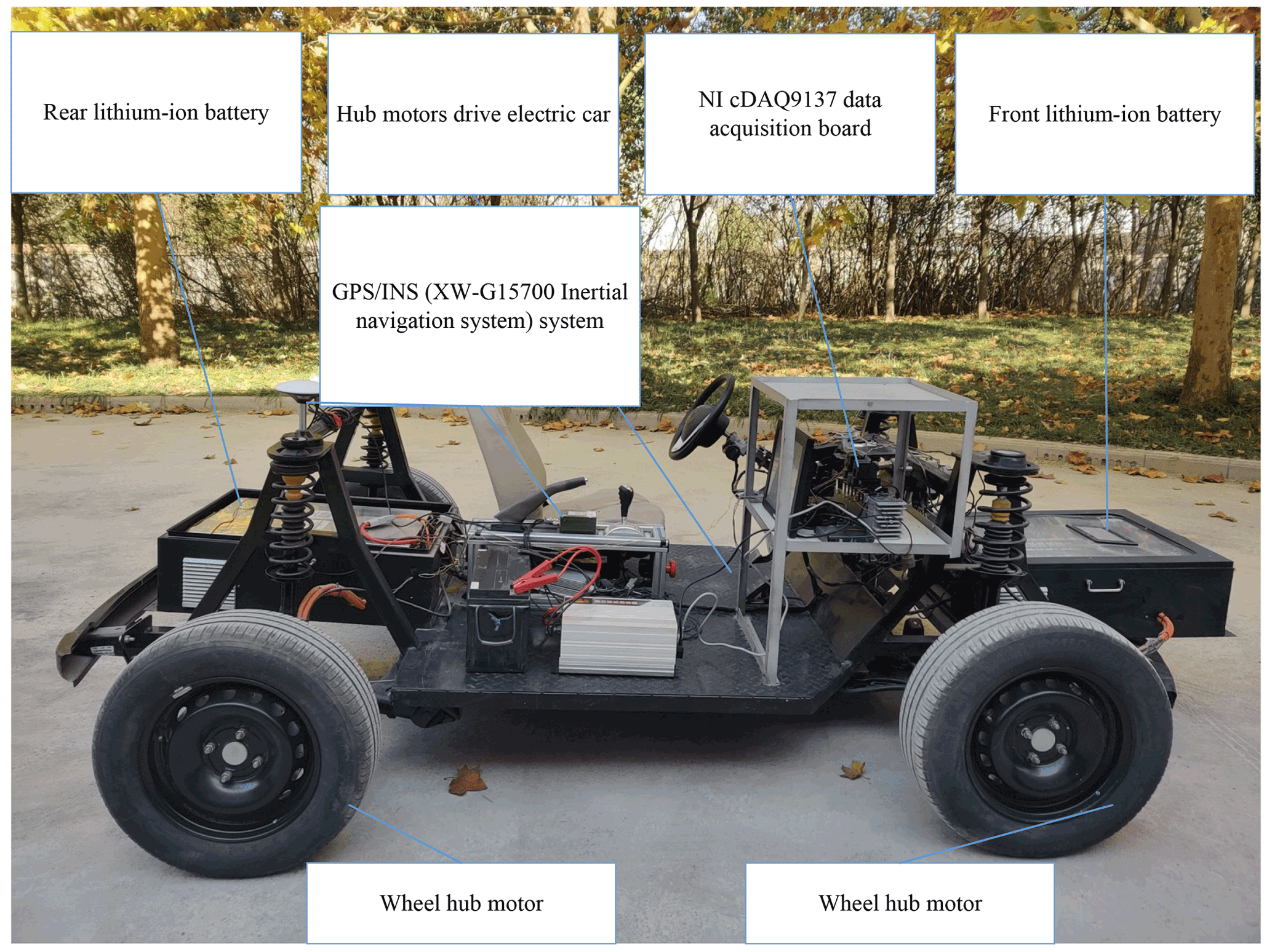
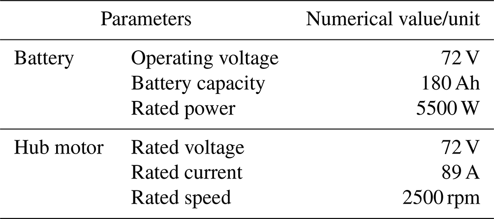
In order to verify the robustness and accuracy of the road adhesion coefficient estimator, a four-wheel-hub-motor vehicle test platform was built for this work. This platform is mainly divided into four parts: the vehicle chassis, the hub-motor drive system, the energy management system and the control system. The hub-motor test car is shown in Fig. 9. The power supply for the hub-motor vehicle is provided by two sets of 72 V battery packs, which mainly service the three electrical components, including the four hub motors, the electric power steering and the controller. Among these components, the hub motors use a DC brushless motor. The main vehicle structure parameters are shown in Table 2.

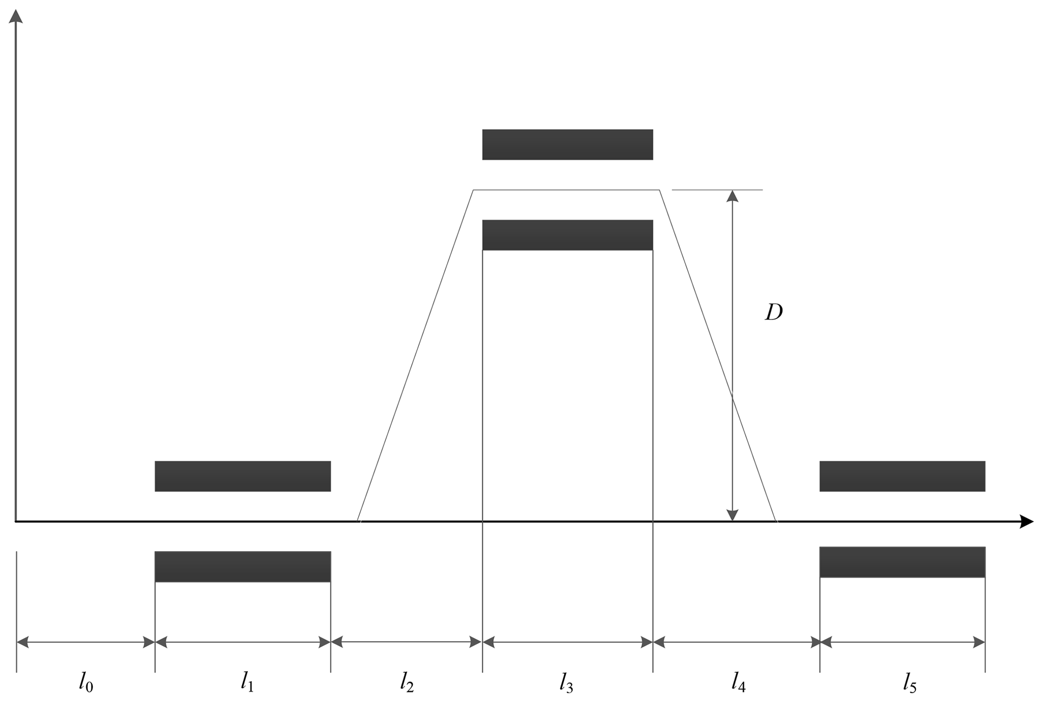
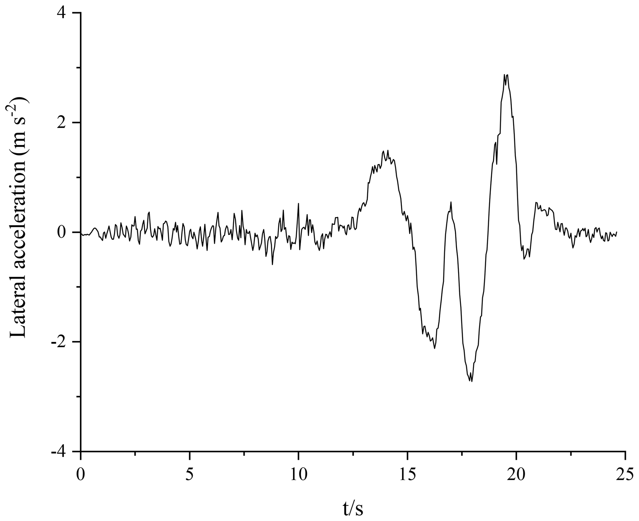
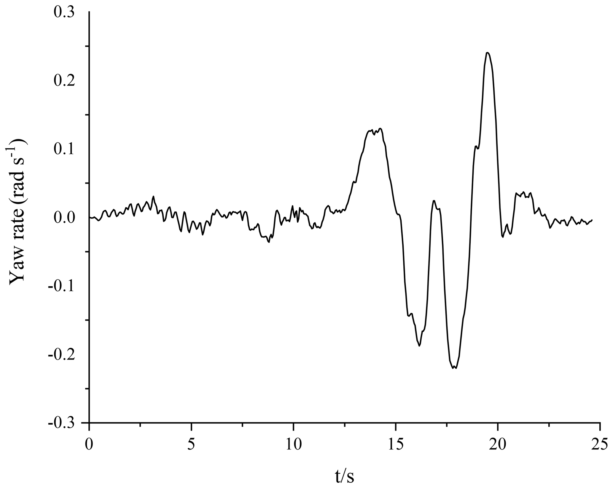
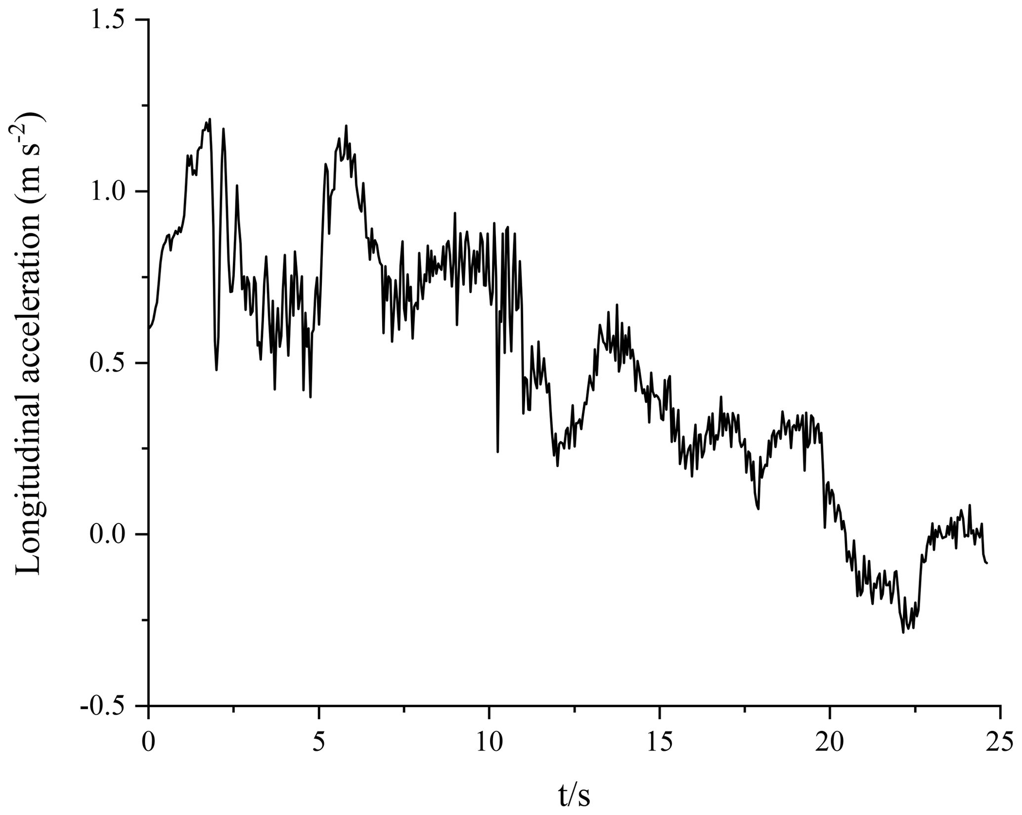
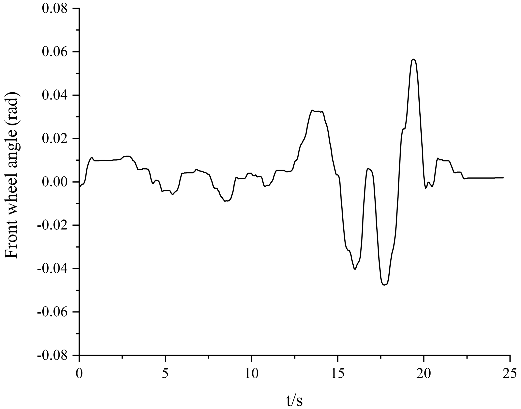
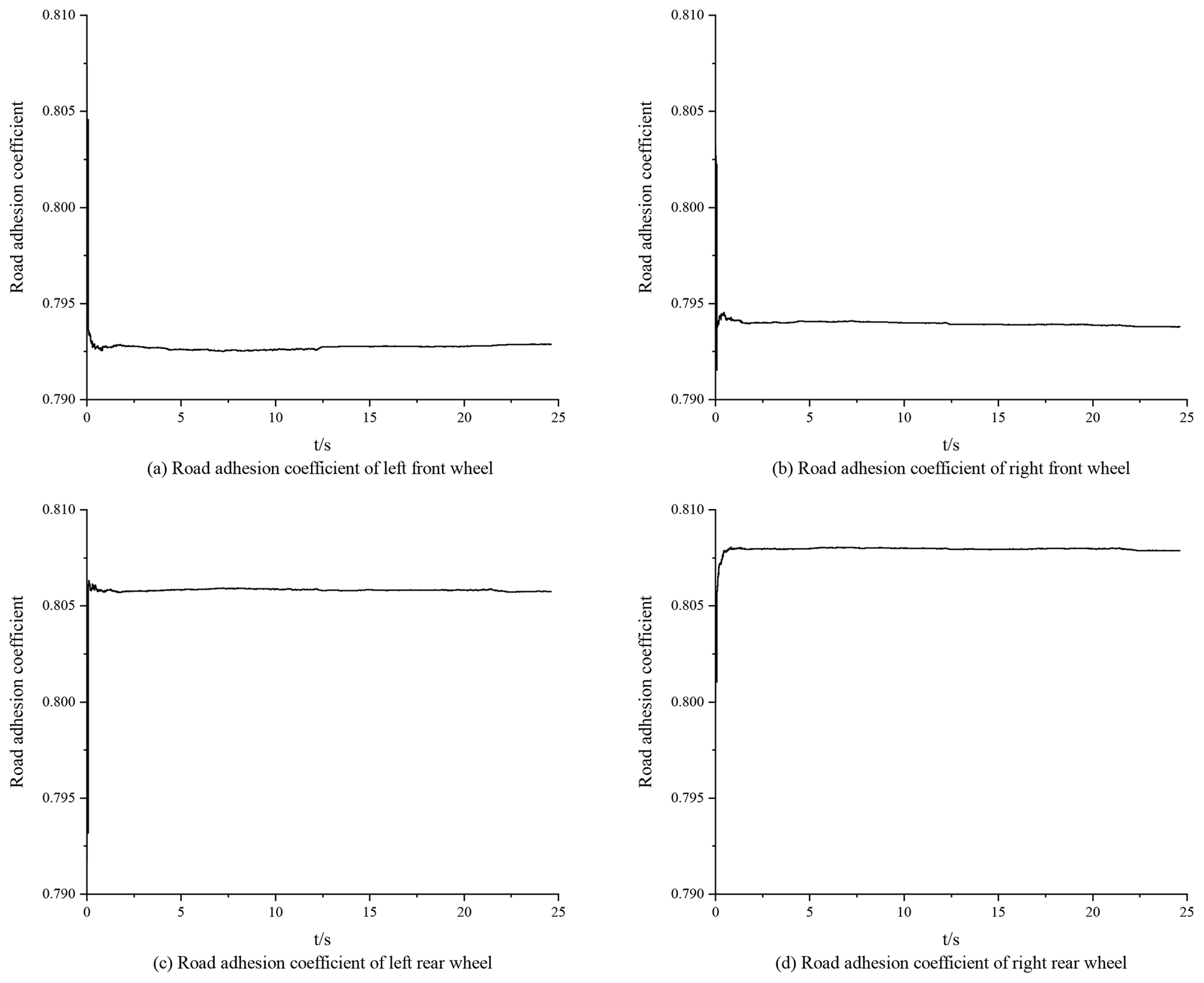
In the vehicle driving experiment, the sensors used mainly included components such as a three-axis accelerometer, a fiber-optic gyroscope, a wheel speed sensor, a steering angle sensor and a speed sensor based on GPS. The vehicle is equipped with an XW-G15700 inertial navigation system and a satellite navigation system. The longitudinal acceleration and lateral acceleration data are obtained by the integrated GPS/INS navigation system. The yaw rate is obtained by the fiber-optic gyroscope sensor, and the front-wheel angle is obtained by the R100 series angle sensor. The vehicle-mounted test system is equipped with an NI data acquisition (DAQ) device for signal processing and data acquisition, and it uses a LabVIEW serial port communication VISA module to achieve communication with the NI cDAQ9137 data acquisition box. According to the above simulation results, the PF algorithm shows good robustness. Therefore, in the road test of real vehicles, the PF algorithm is used to estimate the road adhesion coefficient. Based on the hub-motor vehicle test platform, a road test using a real vehicle was carried out on dry pavement under double-lane-changing conditions. To ensure driving safety, the speed is set as 40 km h⁻¹. The double-lane-changing working condition is shown in Fig. 10. The specific settings of this working condition are as follows: D=3.5 m; l₁=15 m; l₂=30 m; l₃=25 m; l₄=25 m; l₅=30 m; the l₀ setting is related to vehicle speed v_x, and l₀=2v_x; due to the limited test site, the track can only be composed of a surface with the same friction level; and the road adhesion coefficient is approximately μ≈0.8. The obtained data are shown in Figs. 11–14, and the experimental results are shown in Fig. 15.

According to Fig. 15, in the experimental process, the estimator based on the PF algorithm can realize road surface identification with an error of less than 1 %, which verifies the feasibility and effectiveness of the algorithm with respect to estimating the road adhesion coefficient and shows good robustness.

6 Conclusions

In this paper, a 7-DOF vehicle model and the Dugoff tire model are established using the MATLAB–Simulink software platform. Based on the UKF algorithm and PF algorithm, road adhesion coefficient estimators are designed, and simulation experiments are carried out. In order to verify the feasibility and robustness of the algorithms on a real road, a hub-based motor vehicle test platform is built to complete real-vehicle experiments, and the following conclusions are drawn:

• a.

  The simulation results of high- and low-adhesion-coefficient roads show that the estimation of the road adhesion coefficient based on the UKF and PF algorithms can show good robustness and that these algorithms can quickly and effectively estimate the road adhesion coefficient. Via comparative analysis, it is found that the estimation of the road adhesion coefficient based on the PF algorithm is more accurate than that of the UKF algorithm, and the former also has a better robustness and control effect.

• b.

  Via the actual vehicle verification, it is found that the road adhesion coefficient estimator designed based on the PF algorithm can effectively and accurately complete road adhesion coefficient estimation. The experimental results show that the method has good robustness.

In view of the limitations of the KF algorithm, this paper applies the PF algorithm to the estimation of the road adhesion coefficient. The estimator based on the particle algorithm is not limited by the noise type nor the system model, which can improve the accuracy of the road adhesion coefficient. However, the estimator based on the particle algorithm has a large computational burden as well as certain limitations with respect to real-time performance. In addition, the multi-information and multi-method fusion estimation method is not used to estimate the road adhesion coefficient. Therefore, in order to obtain a real-time and accurate road adhesion coefficient, using vehicle dynamics model and multi-sensor information fusion technology, with a modeling analysis method, future work will focus on parameter estimation theory, adaptive control theory, simulation analysis and other means combined with a dynamic tire friction model in order to identify and predict various road conditions under arbitrary vehicle working conditions.