the Creative Commons Attribution 4.0 License.
the Creative Commons Attribution 4.0 License.
 | 23 Feb 2023
Decoupling active disturbance rejection trajectory-tracking control strategy for X-by-wire chassis system
Haixiao Wu
Yong Zhang
Fengkui Zhao
Pengchang Jiang
Due to the inherent dynamic coupling between mechanical components such as the steering system and suspension system, the vertical external input will affect the lateral movement of the chassis, which makes it difficult to track the ideal trajectory when complex excitation conditions exist. To solve the abovementioned problems, the X-by-wire chassis is taken as the research object in this work, and the coupling dynamic model is established. Then, based on proving the reversibility of the coupling dynamic model, a pseudo-linear composite system is proposed to decouple the lateral and vertical signals of the chassis system. Next, the decoupling active disturbance rejection (DADR) trajectory-tracking control strategy is proposed. And a multi-objective optimization method of the bandwidth parameters of the DADR trajectory-tracking controller is proposed according to its convergence conditions. Experiments show that the proposed control strategy can effectively suppress the vehicle roll and yaw motion caused by the lateral–vertical dynamic coupling in the process of trajectory tracking to realize the accurate tracking of the ideal trajectory.
- Article
(8942 KB) - Full-text XML
- BibTeX
- EndNote


Automatic lane-change maneuvers and obstacle-avoidance systems can effectively reduce the incidence of vehicle collision accidents caused by human behavior to further improve traffic safety (Liu et al., 2020; Ji et al., 2019). The achievements of automatic lane-change maneuvers and obstacle-avoidance depend on the high-precision tracking of ideal signals in chassis steering, braking, and other subsystems. However, when tracking obstacle avoidance trajectories in complex traffic environments, the trajectory-tracking accuracy and response speed will be affected by both sides of external factors, including random road input, lateral wind, etc., and internal factors, such as vertical and lateral dynamic coupling characteristics. Because of these factors, it is difficult to provide accurate and fast actuator responses in the process of vehicle trajectory tracking (Wang et al., 2017). Therefore, how to design the lane-change trajectory-tracking control strategy, considering the external disturbance of the vehicle in complex traffic environments and the vehicle chassis dynamic coupling, is the key point for the intelligent vehicle to ensure safety and stability for lane-change maneuvers.
Existing research on trajectory-tracking control mainly focuses on local trajectory replanning and hierarchical control under random disturbances (Yue et al., 2019; Wang et al., 2019). In Yue et al. (2019), aiming at a highway tire burst, a hierarchical control framework for vehicle automatic risk-avoidance trajectory planning and tracking is proposed. Wang et al. (2019) solve the problem of the full-state regulation control of asymmetric under-actuated surface vehicles under disturbance. The above studies effectively suppress fluctuations in the trajectory-tracking process under disturbance. However, due to lateral and vertical dynamic coupling, signal disturbance on lateral or vertical motion cannot be suppressed independently, and active inputs of steering and suspension systems will simultaneously affect vehicle lateral and vertical dynamics (Wang et al., 2018). For instance, the active roll control moments from the chassis controller will not only affect the vertical signals, such as the roll angular velocity, but also change the lateral dynamic parameters, such as yaw angular velocity. Besides, disturbance compensation in trajectory-tracking control has been widely studied (Fiengo et al., 2019; Wang et al., 2019). However, if the compensation control signal changes rapidly, then it is difficult to achieve desired control performance due to lateral and vertical dynamic coupling.
Compared with conventional chassis technology without active control, the advanced X-by-wire chassis enables the active control of roll torque, yaw torque, and front wheel angle. Therefore, the trajectory-tracking control of the X-by-wire chassis system is a typical multivariable control system (Ni et al., 2019). Specifically, when the vehicle equipped with an X-by-wire chassis tracks the curve trajectory, then the dynamic coupling on the signal layer will cause interference in the mechanical layer. For example, the road excitation signal will affect the yaw motion and roll motion of the vehicle with the X-by-wire chassis system. To eliminate the coupling between inputs and outputs, decoupling methods, such as artificial neural network decoupling, robust decoupling, fuzzy decoupling, and inverse system decoupling, are commonly used in multivariable control systems (Zhao et al., 2019; Wu et al., 2020). In Zhao et al. (2019), to solve the vibration problems caused by the nonlinear coupling of longitudinal, lateral, and vertical dynamics, a hierarchical integrated controller for distributed electric vehicles is proposed to improve driving safety. Wu et al. (2020) propose a sliding-mode decoupling control strategy for an electric wheel vehicle based on the inverse system method. However, the abovementioned decoupling control strategies are not applicable for curve trajectory-tracking problems in real complex traffic environments. Because these strategies do not take the trajectory-tracking accuracy and response speed into account in the lane-change obstacle-avoidance process, the disturbance suppression of excitation signals under uncertain environmental conditions is also excluded. In recent years, active disturbance rejection control (ADRC) has been proposed and applied to the tracking problem of multivariable control systems. In Luo et al. (2018), a feed-forward coupling compensation decoupling control method based on ADRC is proposed to solve the cross-coupling problem caused by variable wind disturbance in the system. In Zhang and Chen (2016), based on ADRC feedback linearization, a feed-forward controller based on an equivalent error model is designed to further improve the tracking performance of the system. In Xia et al. (2016), a tracking control method of an automatic land vehicle (ALV) lateral motion is proposed, and the ADRC is used to ensure the control accuracy and robustness. To some extent, the above methods have solved the performance robustness of the controller in the presence of disturbances and the coupling problem caused by the disturbance input but cannot solve the problem of the internal dynamic coupling of the system, so it needs to be further studied.
To solve the above problems, a decoupling active disturbance rejection (DADR) trajectory-tracking control strategy is proposed. First, based on the inverse system theory, the decoupled pseudo-linear composite system is constructed to decouple the input and output signals of the original system. Then, for the decoupled pseudo-linear system, independent lateral motion and vertical motion DADR trajectory-tracking controllers are used. And a multi-objective optimization method of bandwidth parameters of the DADR trajectory-tracking controller is proposed according to its convergence conditions. Finally, through the experimental verification on the hardware-in-the-loop test platform, it is proved that the strategy proposed in this work not only can effectively improve the trajectory-tracking performance under road excitation but also significantly inhibits the roll motion of the vehicle when tracking the curve trajectory in order to improve the ride comfort. The decoupling active disturbance rejection (DADR) trajectory-tracking control strategy proposed in this work and its hardware in the loop (HIL) test platform are shown in Fig. 1.
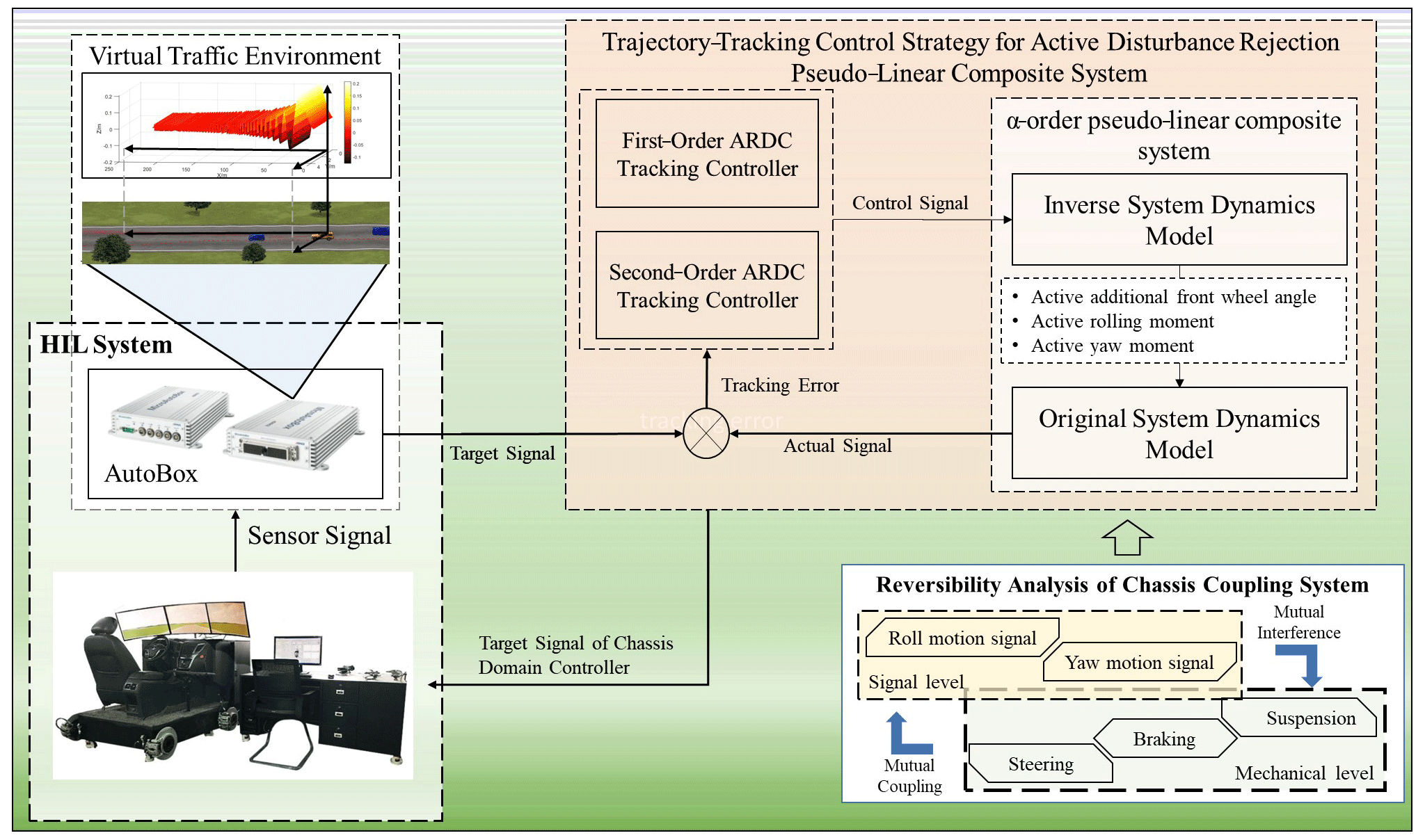
Figure 1The decoupling active disturbance rejection (DADR) trajectory-tracking control strategy proposed in this work and its hardware in the loop (HIL) test platform.
The main contributions of this paper are as follows:
-
The chassis system's yaw signal and roll signal are decoupled on the signal layer so that the yaw motion or roll motion of the chassis system can be compensated and controlled independently. Furthermore, in the mechanical layer, the cooperative control of the chassis mechanical components in the steering-by-wire system, braking-by-wire system, and active suspension system can be realized.
-
The system reversibility is analyzed and verified based on the coupled lateral and vertical dynamic model, and the α-order chassis pseudo-linear composite system is obtained to decouple the lateral and vertical signals of the chassis system.
-
A decoupling active disturbance rejection (DADR) trajectory-tracking control strategy is proposed, and a multi-objective optimization method of bandwidth parameters of the DADR trajectory-tracking controller is proposed according to its convergence conditions.
The rest of this paper is arranged as follows: Sect. 2 is the modeling of the X-by-wire chassis and its analysis in the trajectory-tracking task. Section 3 proposes the decoupling active disturbance rejection (DADR) trajectory-tracking control strategy. Section 4 presents the results and discussion. Section 5 is the conclusion.
To analyze the mechanism of lateral and vertical dynamic coupling, this section first establishes the X-by-wire 3 DOF (degrees of freedom) coupled dynamic model, including the input signals of the active roll torque, yaw torque, and front wheel angle, as shown in Eq. (1).
where δ is the differential steering compensation angle signal of the front wheel, Tz is the yaw torque signal, and Tϕ is the roll torque signal of the suspension system. m is the vehicle mass, ms is the sprung mass, mf is the front unsprung mass, and mr is the rear unsprung mass. a is the distance from the center of mass to the front axle, b is the distance from the center of mass to the rear axle, Iz is the yaw moment of inertia, Ix is the roll moment of inertia, Ixz is the inertia product of the yaw motion, h is the roll center height, kf is the front wheel yaw stiffness, kr is the rear wheel yaw stiffness, Ef is the front roll steering coefficient, Er is the rear roll steering coefficient, vx is the longitudinal speed of the vehicle, β is the sideslip angle of the centroid, ωr is the yaw rate, ϕr is the roll angle, Kϕ is the suspension roll stiffness coefficient, Dϕ is the suspension roll damping coefficient, and δd is the front wheel angle applied by the driver.
The state variable of the coupled chassis system is , the control input signal is , and the system output signal is . The state space of the system is shown in Eq. (2).
Then, the trajectory-tracking task is analyzed based on the above dynamic model, which is shown in Eq. (2). For the trajectory-tracking task, the goal is to eliminate the error between the actual trajectory and the ideal trajectory e. For the chassis motion control task, the goal is to eliminate the error between the ideal front wheel angle and the actual front wheel angle. Therefore, it is necessary to establish the relationship between the trajectory-tracking error and the ideal front wheel angle.

The required front wheel angle to track a given path is calculated based on a pure pursuit algorithm (Yamasaki and Balakrishnan, 2010), as shown in Eq. (3).
where δi is the ideal front wheel angle, L is the wheelbase, e is the lateral error between the current vehicle attitude and the target waypoint, vx is the longitudinal speed of the vehicle, and kv is the adjustment factor for the tracking process.
Next, ideal signals for the trajectory-tracking task are analyzed and listed as follows: tracking the desired trajectory is done by controlling the front wheel rotation angle and maintaining the roll angle as 0. For the X-by-wire chassis system, the target trajectory should be converted into the target yaw angle, as shown in Eq. (4) (Wang et al., 2018).
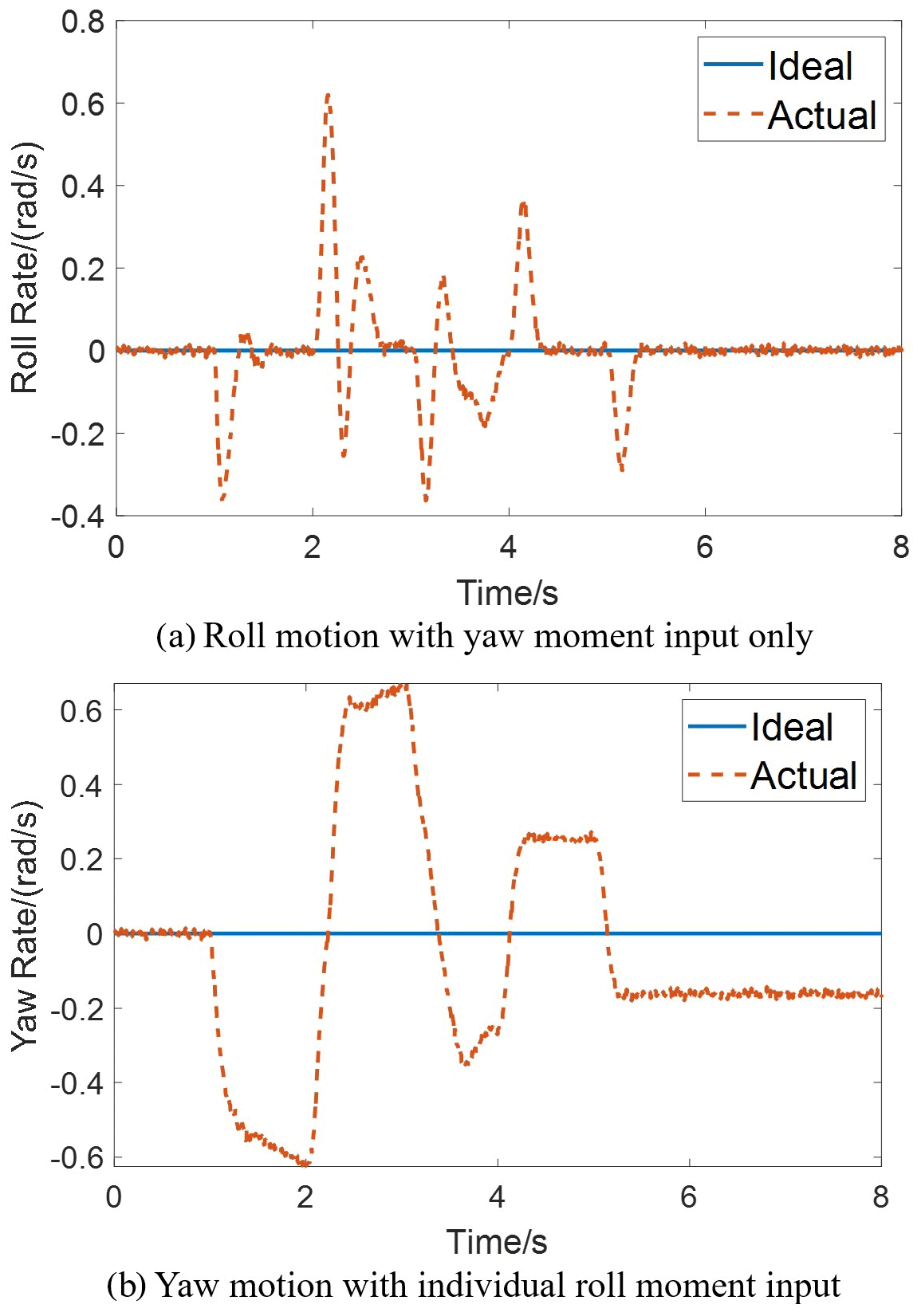
Based on the dynamic model without any decoupling transformation, the above trajectory-tracking control tasks are analyzed, and the results are shown in Fig. 3. It can be seen that the lateral motion and vertical motion of the chassis system cannot be controlled separately and are coupled with each other. In other words, the lateral motion cannot be corrected separately without affecting the vertical motion, and vice versa.
In this section, to suppress the random roll motion caused by the coupling of lateral and vertical dynamic signals during the trajectory tracking, a decoupling active disturbance rejection (DADR) trajectory-tracking control strategy is proposed. The control strategy is shown in Fig. 4. First, the α-order pseudo-linear composite chassis system is obtained, which decouples the input signal and output signal of the coupling system. Then, a trajectory-tracking control strategy with DADR for the pseudo-linear composite system is proposed, which can realize the independent anti-interference control of the lateral or vertical motion of the chassis system. Next, the convergence of extended-state observer (ESO) is verified, and a multi-objective optimization method based on bandwidth parameters of the DADR trajectory-tracking controller is proposed according to its convergence conditions, which can demonstrate that the system has better anti-interference performance in the process of trajectory tracking.
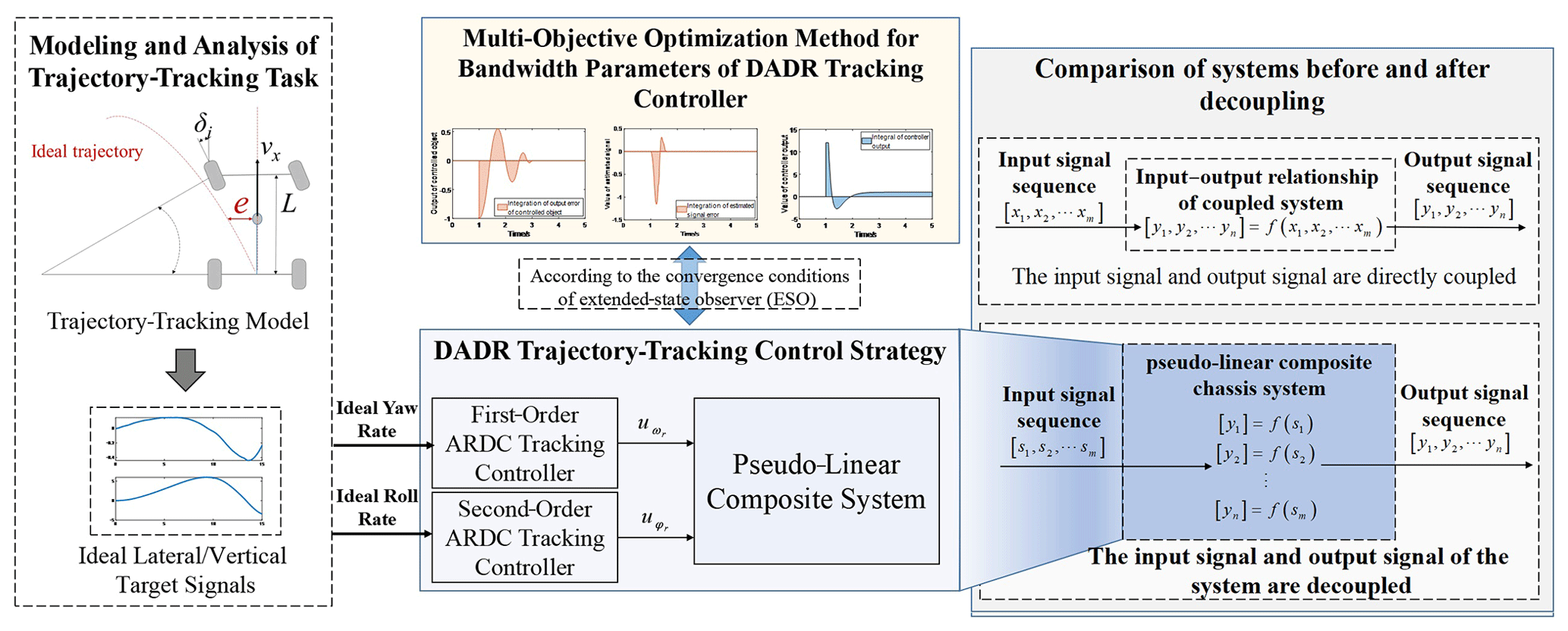
Figure 4Decoupling active disturbance rejection (DADR) trajectory-tracking control strategy.
3.1 DADR trajectory-tracking control strategy for the pseudo-linear composite system
To complete the abovementioned control tasks, a pseudo-linear composite system is established by constructing an inverse system, which realizes the decoupling of lateral and vertical input and output. To build the inverse system, the system reversibility is first proved by introducing the following definitions and lemmas.
Definition 1 (Wu et al., 2020) is that nonlinear systems will be reversible if the system has a relative order vector, as in Eq. (5).
where αi is the relative order vector of the original system, and i is the ith output signal of the system.
If , then the system is reversible. n is the matrix order of the original system.
Lemma 1 (Wang et al., 2018) is created, for which the existence condition of the relative order vector is presented. We continuously derive the system output variable until each component in can contain the input u, and is the full rank of the Jacobian matrix of the input u; then, the system has a relative order vector, as in Eq. (6).
Based on Definition 1 and Lemma 1, the system reversibility of the coupled chassis system is proved.
First, the output signal of the lateral and vertical coupled chassis system is obtained from Eq. (2). According to Lemma 1, the derivative of the output vector , with the input vector u, is calculated, as shown in Eq. (7).
The relative order vector is discussed according to Lemma 1. Assuming , the rank to the Jacobian matrix of the control input u is shown in Eq. (8). The first derivative equation of y1 contains the control input u for the first time, and the Jacobian matrix of Y1 to u is full rank, so that α1=1.
Next, assuming , the rank of the Jacobian matrix of u is shown in Eq. (9). The first derivative equation of y2 contains the input u for the first time, and the Jacobian matrix of Y2 to u is full rank, so that α2=1.
Assuming , the rank of the Jacobian matrix to u is shown in Eq. (10). The second derivative equation of y3 contains the input u for the first time, and the Jacobian matrix of Y3 has full rank to u, so that α3=2.
From Lemma 1, since the Jacobian matrix of to u is full rank, the system has a relative order vector, as shown in Eq. (11).
According to Definition 1, . Therefore, the original integrated chassis system is reversible. The decoupling of the coupled signals in the original chassis system can be achieved by establishing an inverse system.
According to the above analysis, the coupled chassis system is reversible, which means the input and output signals of the original system can be decoupled by establishing a pseudo-linear composite system to achieve the compensation control for trajectory tracking. Then, the inverse system model of the coupled chassis system and the α-order pseudo-linear composite system will be established and analyzed. The following definitions and lemmas are introduced to present the derivation process.
For Lemma 2, in the α-order inverse system, the operator θ is used to represent the input–output relationship of a nonlinear system Σ with p-dimensional input and q-dimensional output, as shown in Eq. (12).
where u is the control input of the original system, and y is the control output of the original system.
Assuming Πα is a system with q input and p output, the mapping relationship between input and output is shown in Eq. (13).
where is a differentiable function vector whose initial value satisfies the initial value condition of the original nonlinear system Σ, and φi is defined as the αi-order derivative of ydi, as Eq. (14).
And if the operator in Eq. (11) satisfies the condition in Eq. (15), then the following applies:
Then, the system Πα is regarded as the α-order inverse system of the original nonlinear system Σ.
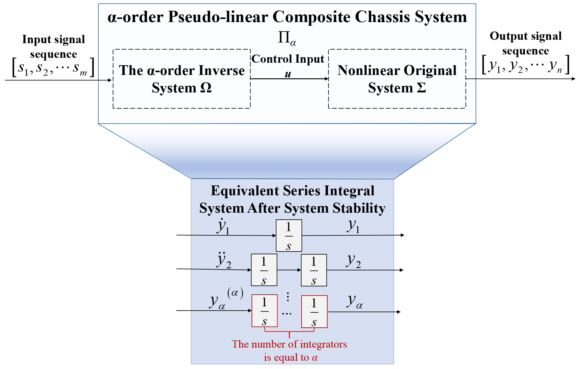
Definition 2 is the α-order pseudo-linear composite system. If the system Ω is a composite system , with a similar linear transfer relationship composed of the α-order inverse system and the nonlinear original system Σ in series, then the system Ω is called the α-order pseudo-linear composite system.
The original multi-input–multi-output nonlinear system has been linearized and decoupled into q independent linear integral systems. The composite system is equivalent to several connected integrators in series, and its input and output are shown in Eq. (16).
Based on Definition 2 and Lemma 2, the inverse system model of the coupled chassis system is deduced, and then the input and output characteristics of the α-order pseudo-linear composite system are analyzed.
As shown in Eq. (2), the output of the nonlinear original system Σ is . From Lemma 2, the output of the α-order inverse system Πα is the control input u of the original system, as shown in Eq. (17).
where
Then the state space of the inverse system is shown as Eq. (18).
where
Next, based on the inverse system derived above and the original coupling system, the decoupled pseudo-linear composite system is obtained. The input and output characteristics of the α-order pseudo-linear composite system Πα are presented and analyzed, as shown in Fig. 8. As shown in Fig. 5, the α-order pseudo-linear composite system Πα is composed of the α-order inverse system Ω and the nonlinear original system Σ in series. So the original system can be equivalent to the series integral system, which is easier to design the tracking controller.
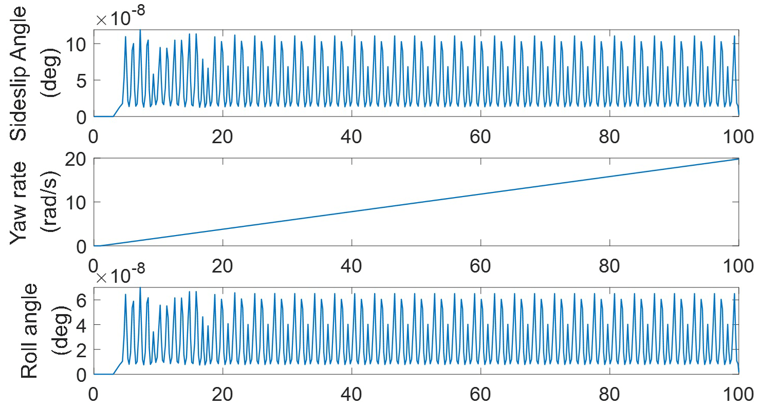
For instance, with a single yaw signal input in the α-order pseudo-linear composite system, only the corresponding output value changes accordingly, and the other outputs are not affected, as shown in Fig. 6. However, although the coupled system was decoupled, some fluctuations in the other outputs still exist. And such fluctuations will be worse under road disturbance, which should be should be taken into consideration in the controller design.
Next, the trajectory-tracking control strategy is designed. The purpose of the trajectory-tracking control task is to track the desired trajectory by controlling the front wheel angle and suppressing the random roll motion caused by road disturbance. To realize the above control task, a trajectory-tracking control strategy with decoupling active disturbance rejection (DADR) for the pseudo-linear composite system is proposed, as shown in Fig. 7. The lateral and vertical tracking controllers are designed separately through an active disturbance rejection control algorithm to achieve anti-interference tracking of the ideal trajectory and suppress the vertical motion at the same time.
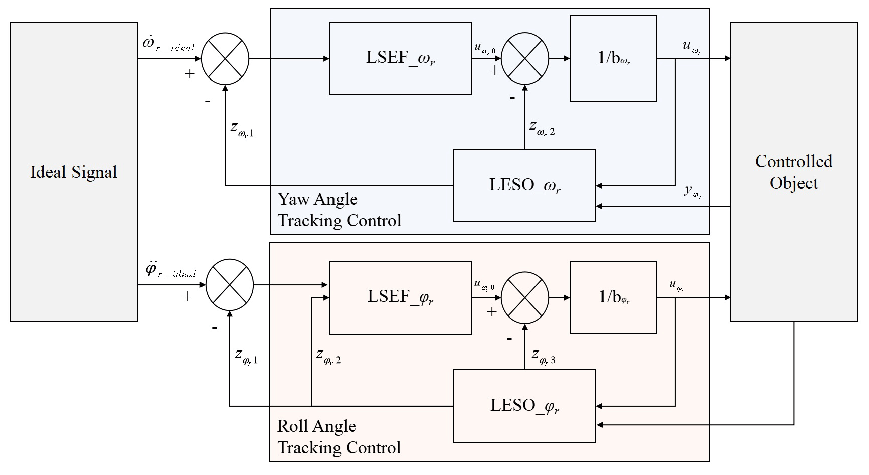
Figure 7Trajectory-tracking controller with active disturbance rejection for a pseudo-linear system.
The standard form of the active disturbance rejection control algorithm for α-order systems is first discussed. As shown in Eq. (19),
where α is the order of the system, b is the control variable gain, y is the system output, w is system interference, and t is the time-varying state of the system. The interference sources are analyzed, including the external road input, crosswind, and other interference, as is the interference caused by the measurement error within the sensor inside the system.
Since the control variable gain b in Eq. (19) is difficult to obtain in the real control system, the estimated value b0 is commonly used. And the disturbance caused by the inaccurate estimation is added to the total disturbance to realize the suppression of interference signals, such as road noise in the trajectory-tracking process, as shown in Eq. (20).
The state space of the α-order controlled object is shown in Eq. (21).
where
The observer of the controlled object is shown in Eq. (22).
where L is an adjustable parameter in the state observer. A, B, L, and C are integrated into Eq. (20) to obtain the extended-state observer, as shown in Eq. (23).
As in Eq. (23), when ESO reaches the design goal, the last output of the extended-state observer zα can track the real error f of the system. Therefore, the control law can be designed, as shown in Eq. (24), to achieve the control task.
By substituting Eq. (24) into Eq. (20), Eq. (25) can be obtained.
From the input–output relationship of the α-order pseudo-linear composite system Πα, the yaw rate control can be regarded as the first-order system control, and the roll angle control is the second-order system control. Therefore, for the yaw rate control, the state error feedback (SEF) control law SEF_ωr is shown in Eq. (26).
The yaw rate control extended-state observer ESO_ωr is shown in Eq. (27).
For the roll angle control, the state error feedback control law SEF_φr is shown in Eq. (28).
The roll angle control extended-state observer ESO_φr is shown in Eq. (29).
When the roll angle control extended-state observer ESO_φr converges, then will converge to , and will converge to . The roll angle tracking control state error feedback control law SEF_φr and the stabilized controlled object are shown in Eq. (30).
From Eq. (30), the closed-loop transfer function is shown in Eq. (31). The roll angle control extended-state observer ESO_φr works in an ideal state, so the transfer function between r and y is only related to the state error feedback control law. kp and kd directly determine the dynamic system response.
The controller is configured using the bandwidth method. For the controller parameters, the relationship between the bandwidth ωc, kp, and kd is shown in Eq. (32).
It can be seen that ωc corresponds to the cutoff frequency of the second-order system, since the closed-loop cutoff frequency can be applied to evaluate the closed-loop system transient response speed. A positive correlation is shown between the closed-loop cutoff frequency and dynamic system response speed. In addition, by adjusting the closed-loop cutoff frequency, the system is equivalent to a bandpass filter to remove road noise signals in specific frequency bands.
3.2 Extended-state observer (ESO) convergence proof
The DADR-based trajectory-tracking algorithm proposed in this paper has the ability of an anti-interference system because the error in the trajectory-tracking process can be estimated by the extended-state observers, ESO_ωr and ESO_φr, and will be converted to an integrator series system, which is shown in Fig. 5, to achieve the control objectives of removing the interference. In this section, the convergence of ESO is proved, and a multi-objective optimization method of bandwidth parameters of the DADR trajectory-tracking controller is proposed according to its convergence conditions.
The following definitions are introduced to present the proposed controller derivation in detail.
For Definition 3 (Li and Lam, 2013), the linear time-invariant system is shown in Eq. (33).
The necessary and sufficient condition for a system to be asymptotically stable at the origin is that all the characteristic roots of matrix A have negative real parts, and the characteristic polynomial is shown in Eq. (34).
Its n-zero real points λi are completely located on the left half of the plane, as shown in Eq. (35).
Taking the second-order system as an example, the convergence of the roll angle control extended-state observer ESO_φr is proved.
From the equation of the roll angle extended-state observer ESO_φr, the differential equation state estimation can be obtained, as in Eq. (36).
The state estimation error differential equation is established as Eq. (37). With increasing time, the estimation error value will tend to be 0.
The state estimation error is defined as Eq. (38).
From Eqs. (37) and (38), we obtain the following:
The characteristic equation is obtained as Eq. (40). For the differential equation shown in Eq. (40), β1, β2, and β3 are configured according to Definition 3. The eigenvalue can be less than 0 to ensure its convergence and system stability.
The controller parameters are configured using the bandwidth method (Fu and Tan, 2018), as shown in Eq. (41).
The system will be stable if, and only if, ω0>0.
According to Eq. (41), the relationship between the extended-state observer ESO parameter and the observer bandwidth ωo is shown in Eq. (42).
The extended-state observer bandwidth ωo and the controller bandwidth ωc are further discussed. ESO can convert the original problem into a series integrator control problem because the zα of ESO can rapidly suppress the disturbance of the control object, which is equivalent to the inner loop of the controller, so the response speed is faster than the SEF of the outer loop. Therefore, the observer bandwidth ωo should be larger than the controller bandwidth ωc, but the excessive observer bandwidth is difficult to be realized in practical engineering and wastes the control output. In addition, for the controller bandwidth ωc, the excessive bandwidth will also waste the control energy, and it is difficult to suppress the road noise signal of too small a bandwidth (Mosquera-Sánchez et al., 2017; Sahu et al., 2014). To sum up, the objective function in Eq. (43) is established to optimize the extended-state observer bandwidth ωo.
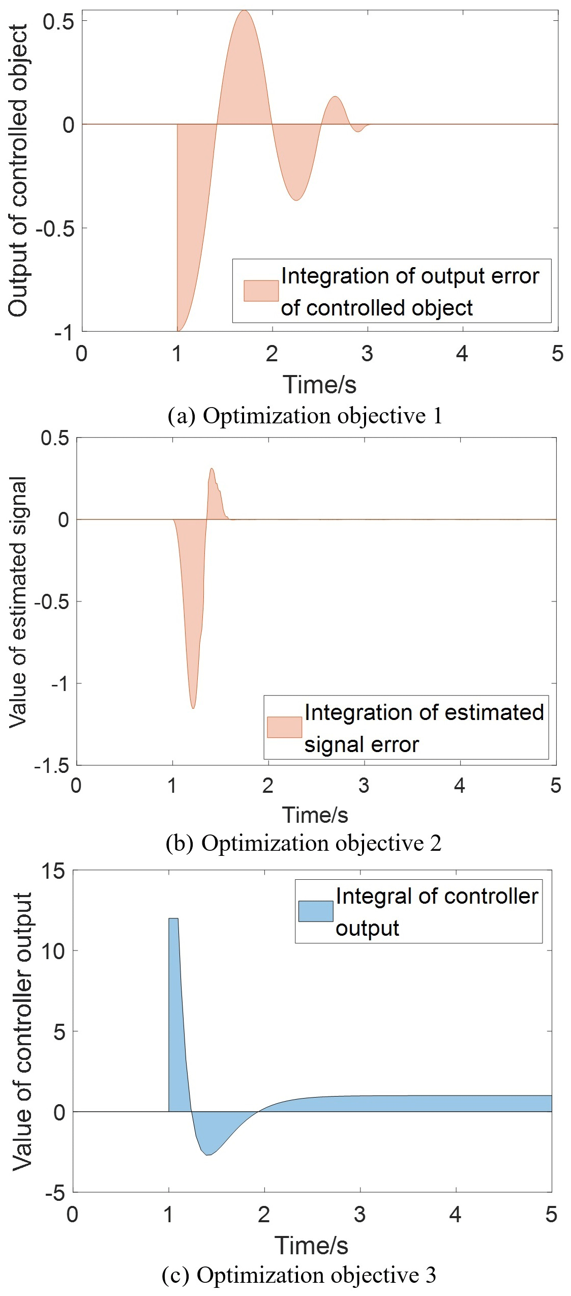
where ωc, ac, and u are design variables to achieve the design goals so that the inner loop responds faster than the outer loop by adjusting the weight parameters. The objective function f1(ωc) represents the difference between the integral of the target signal and the integral of the actual system output. The objective function f1(ωc) is defined to evaluate the system response speed, overshoot, and steady-state error. The objective function f2(ac) is the difference between ∫fideal and ∫zα, which represent the integral of the prior-known noise signal and the integral of the noise observation, respectively. The objective function f2(ac) is minimized to realize fast and accurate noise estimation. The objective function f3(u) is defined as the integral of the controller output. The upper and lower bounds of the constraint are obtained through bench testing and then corrected through multiple tests. The schematic diagrams of these three objective functions are shown in Fig. 8. Due to the relative contradiction between the three objectives, the Pareto solution sets are obtained through iterative optimization, and then the required optimal solution is selected (Rodríguez-Molina et al., 2020; Wu et al., 2019).
The above analysis shows that it will inevitably lead to large controller output if the trajectory-tracking performance needs to be improved. Therefore, a multi-objective particle swarm optimization (PSO) algorithm is applied to optimize these contradictory objectives. The main steps are listed as follows (Zhao et al., 2018).
Step 1 – problem definition. This includes the model definition and algorithm parameters definition.
-
Model definition. This is the optimization objectives, constraints, and design variables.
-
Algorithm parameters definition. This includes the maximum iterations Ite, the number of particles nori, inertia weight w, weight descent rate wdamp, individual learning factor c1, global learning factor c2, and Pareto set threshold nTPareto.
Step 2 – initialization. This is the position and velocity that are assigned for each particle, and the fitness function is calculated.
Step 3 – calculation cycle. This algorithm consists of a PSO module, decomposition module, and Pareto module. The particle velocity, position, and fitness functions are updated by the PSO module. The decomposition module is used to decompose and search the updated particles provided by the PSO module. Finally, the termination conditions are checked, and the Pareto set is obtained (Mac et al., 2018).
Step 4. If the termination conditions are not satisfied, then the iteration process will return to Step 3. Otherwise, the Pareto solution set will be obtained.
The time–frequency domain analysis is conducted in multiple working conditions, and the system dynamic performance of the proposed control strategy is discussed. Then, a hardware-in-the-loop chassis test platform is designed based on dSPACE AutoBox and MATLAB/CarSim software. The proposed control strategy is verified for the lane-changing trajectory-tracking conditions in the established virtual traffic environment. And the simulation results are compared with the neural network proportional integral derivative (PID) control strategy in Wang et al. (2018). It proves that the proposed control strategy can effectively enhance trajectory-tracking accuracy and system anti-disturbance performance.
According to the analysis in Sect. 4, the system's dynamic response performance can be improved by optimizing controller bandwidth parameters and observer bandwidth parameters using a multi-objective optimization algorithm. The multi-objective optimization algorithm parameters are listed in Table 1.
Table 1Initial setting of multi-objective particle swarm optimization algorithm.

The system dynamic behaviors are discussed in the time–frequency domain first. Then, based on the HIL test results, the system response of the proposed control strategy and the neural network PID method are compared and analyzed for the lane-changing trajectory-tracking conditions.
4.1 System dynamic performance simulation in the time–frequency domain
The trajectory-tracking performance and system robustness of the proposed control strategy are discussed based on the time–frequency simulation results. First, from the perspective of the frequency domain analysis, the natural frequencies of lateral vibration and vertical vibration are from 2 to 6 Hz (Morioka and Griffin, 2010; Arnold and Griffin, 2018). The road excitation within this frequency range will result in vehicle resonance, so the controller is required to suppress the signals within the natural frequencies. In this work, the bandwidth method is applied to design the controller's cutoff frequency. The original and optimum Bode diagrams are shown in Fig. 9.
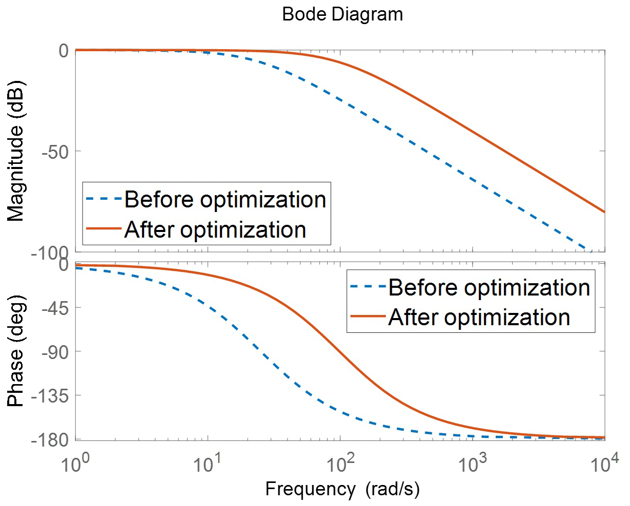
Figure 10 presents the system response in the time domain with the inputs of step signal and the prior-known interference, which verifies the improvement in the system's anti-interference performance. Compared with the benchmark, the dynamic system response speed is dramatically improved by 43.64 %. In addition, the accuracy of the observer state error estimation is improved by 11.93 %. The optimized system can estimate the interference signal faster, which is the foundation of the system simplification and the improvement of trajectory-tracking accuracy.
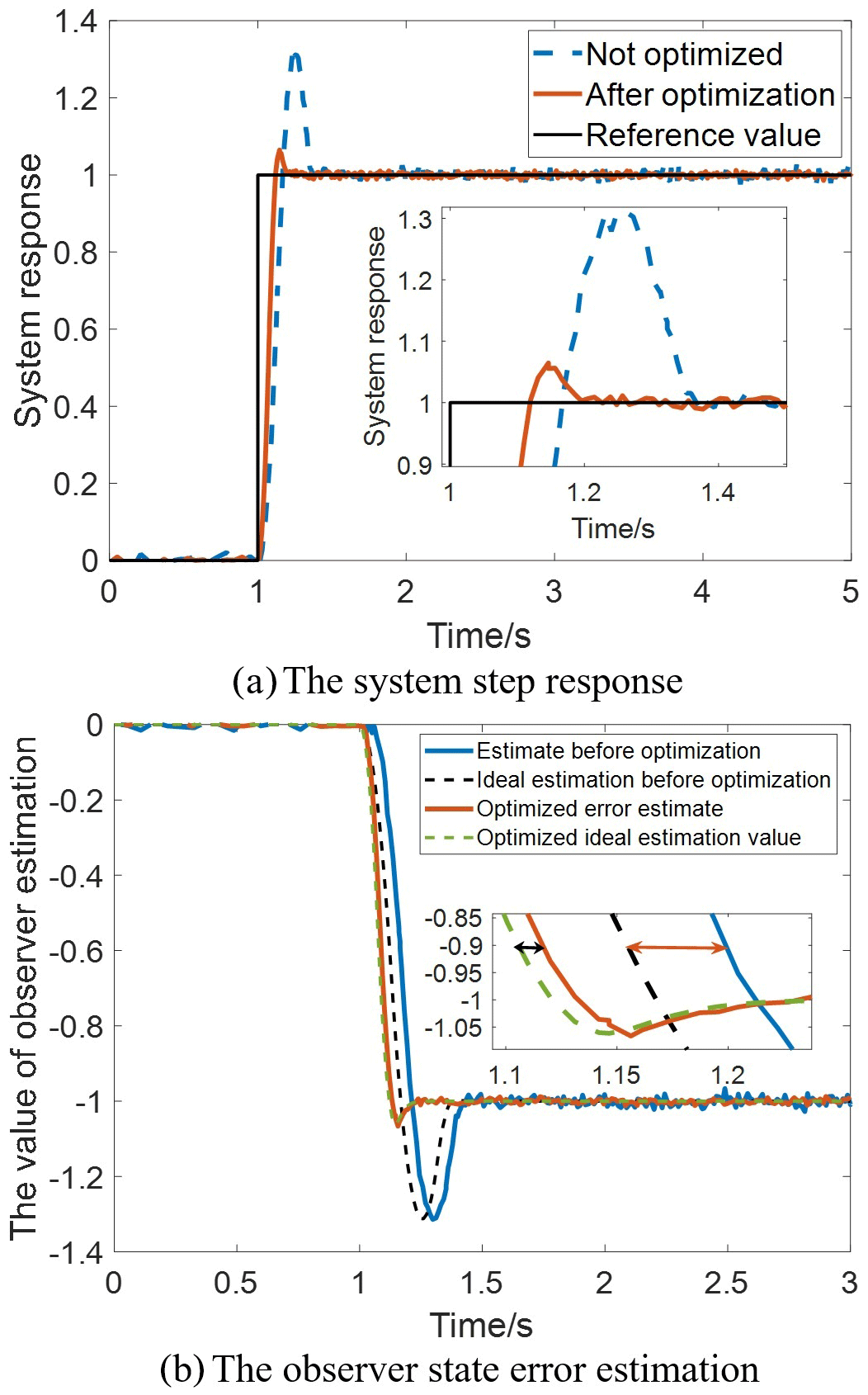
As shown in Fig. 10, the baseline observer has a delay of 0.3 s compared with the target signal. Within 1 to 1.3 s, the system cannot be regarded as a multistage series system, so high-precision control performance is unlikely to be achieved in the baseline observer. However, the optimized system can effectively balance the contradiction of controller bandwidth, observer bandwidth, and control outputs to improve dynamic system performance.
4.2 Trajectory-tracking performance of the hardware-in-the-loop test
In this section, the hardwire-in-the-loop test platform for an X-by-wire chassis is established, based on the MicroAutoBox 1401/1501 (dSPACE GmbH). And the lane-changing trajectory-tracking conditions are established in the virtual traffic environment of MATLAB/CarSim. The effectiveness of the proposed trajectory-tracking control strategy is verified and compared with the neural network PID method in this test platform. The test platform is shown in Fig. 11. The chassis controller output of the platform is collected by the data acquisition card and is transmitted to the vehicle model in the virtual traffic environment. After that, the yaw rate and dynamic model parameters are calculated based on the vehicle model in the virtual traffic environment, which is transmitted to the chassis controller of the real vehicle in real time through the controller area network (CAN) network. This procedure realizes the closed-loop interaction between the real vehicle chassis controller and the virtual traffic environment.
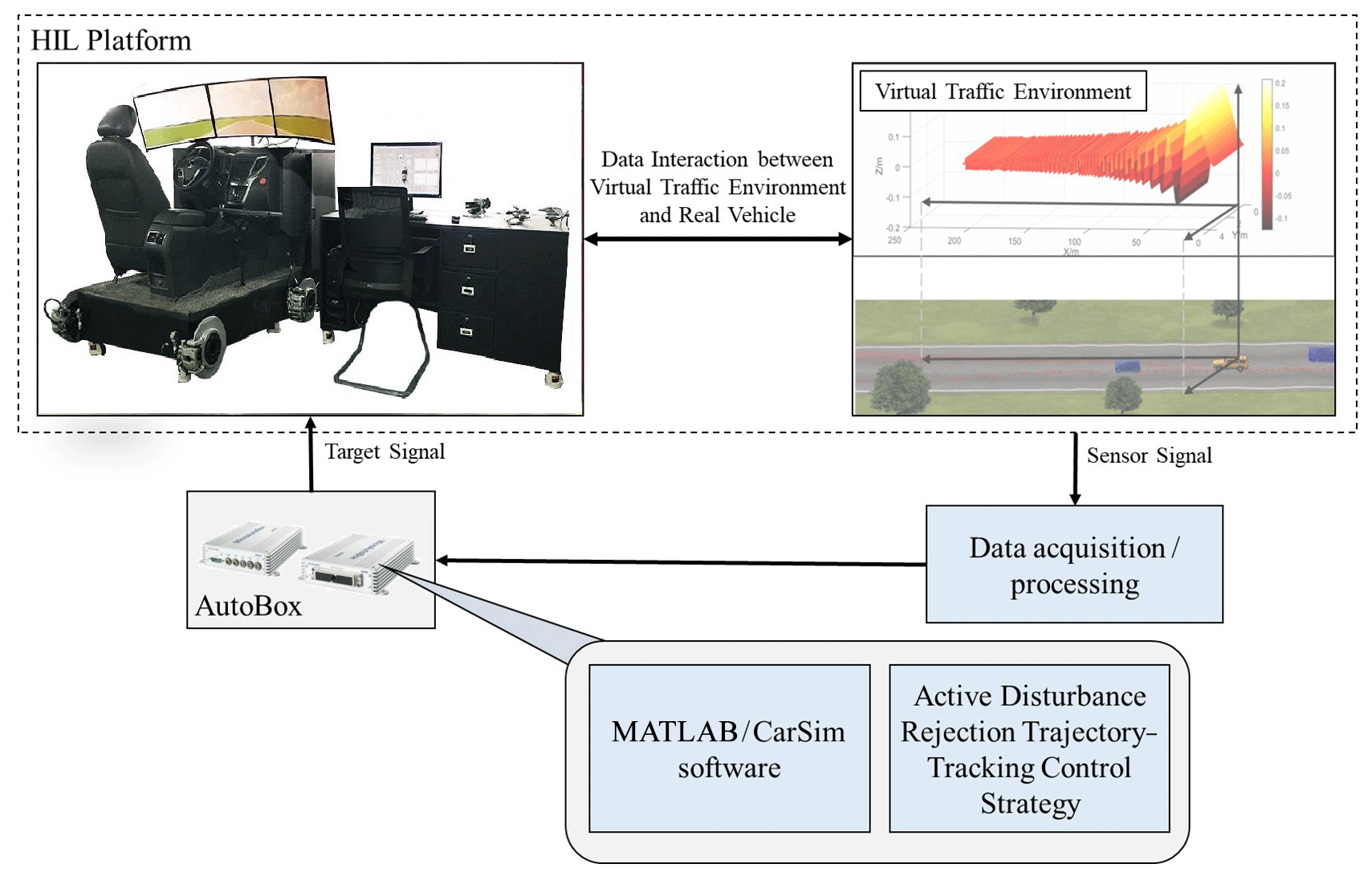
The experimental results are analyzed below and compared with benchmarks. Figure 12 presents the performance of the proposed control strategy on decoupling with uncertain road interference. Both the benchmark and the proposed control strategy can realize the decoupling of lateral and vertical signals. However, in the case of interference, the variance between the actual signal and the ideal signal obtained by the proposed control strategy can be reduced by 51.61 % when compared with that of the benchmark. The mechanism of the above phenomenon is analyzed. The neural network PID inverse system requires a large number of prior-known training data. As for the model uncertainty from road interference, the training dataset is unlikely to cover all the working conditions. Therefore, the neural network PID inverse system cannot eliminate the coupling on the signal layer, which will result in the chassis system interference on the mechanical layer.
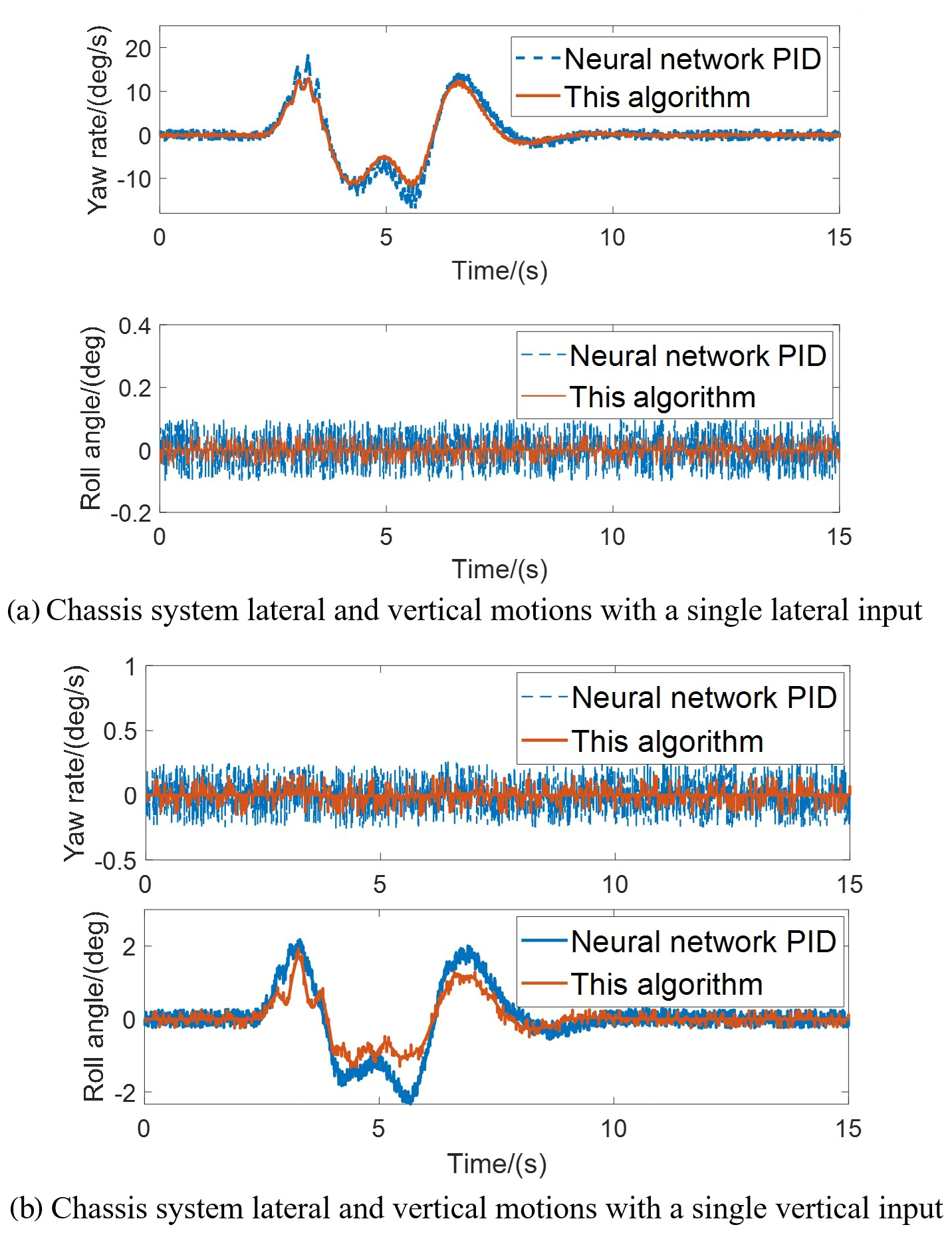
Figure 12The performance of the proposed control strategy on decoupling with the uncertain road interference.
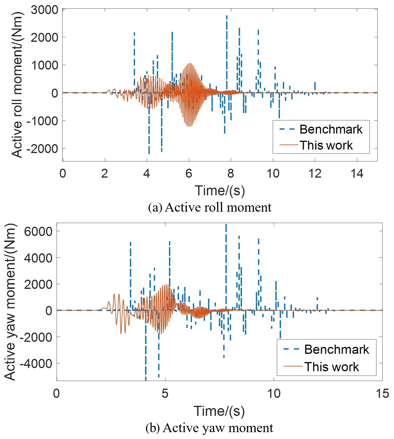
Then, the effectiveness of the proposed trajectory-tracking control strategy is discussed. The active control signals to the controlled object are shown in Fig. 13. The active yaw and roll moment can effectively resist road interferences and enhance the trajectory-tracking performance. Compared with the benchmark, the proposed control strategy can provide a faster response of active yaw moment and roll moment when road disturbances exist. The peak values of active yaw and roll moment obtained by the proposed control strategy can be reduced by 61.45 % and 70.49 %, respectively.
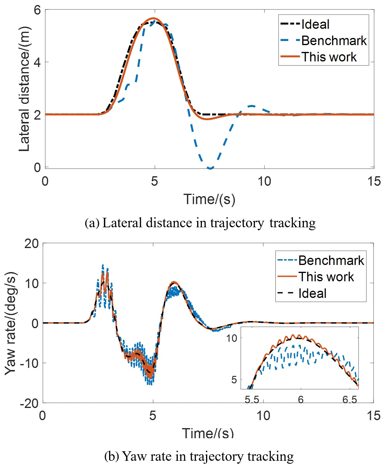
The benefits of the proposed control strategy on the anti-interference ability are compared from the perspectives of the lateral distance and yaw rate in trajectory tracking in Fig. 14. Compared with the benchmark, the proposed control strategy can reduce the trajectory-tracking error by 10.03 %, and the variance of the error within the yaw rate can be reduced by 34.54 %.
From the perspective of vertical motion control, compared with the benchmark, the proposed control strategy can reduce the peak roll angular velocity by 43.64 %. The trajectory-tracking performance on stability is further discussed. The suspension system force and displacement are shown in Fig. 15. The vertical relative displacement of the proposed control strategy is smaller compared with the benchmark. Therefore, the vehicle body behaves more stably with the proposed control strategy in the trajectory-tracking process.

The conclusion can be further verified in Fig. 16. It shows the front wheel angle and lateral acceleration in trajectory tracking. With the same front wheel angle, the lateral acceleration obtained by the proposed control is relatively smaller compared to that of the benchmark. The proposed control strategy can effectively reduce the chassis system interference on the mechanical layer induced by the coupling on the signal layer.
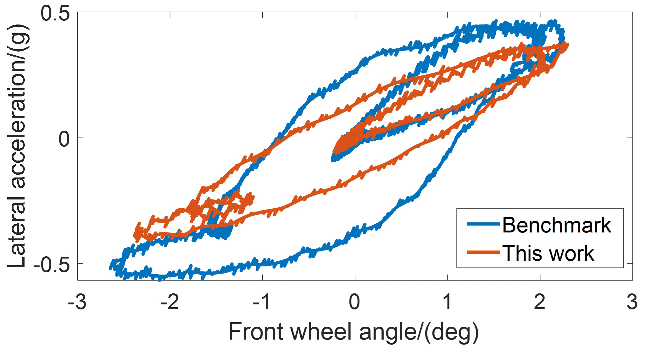
Figure 16Front wheel angle and lateral acceleration of chassis system in trajectory tracking.
In this paper, a coupled dynamic model of the X-by-wire chassis system is established, and the α-order chassis pseudo-linear composite system is obtained. On this basis, a decoupling active disturbance rejection (DADR) trajectory-tracking control strategy is proposed, and a multi-objective optimization method of bandwidth parameters of the DADR trajectory-tracking controller is proposed, according to its convergence conditions.
As far as the results of the simulation and hardware-in-the-loop test is concerned, the trajectory-tracking error within the proposed control strategy can be reduced by 10.03 %, compared with the benchmark, and the variance of the error within the yaw rate can be reduced by 34.54 %. In particular, when road interference existed, the chassis system with the proposed control strategy can track the target trajectory more stably. In addition, the peak value of vehicle roll angular velocity with the proposed strategy can be reduced by 43.64 %. And the relative vertical displacement is remarkably reduced, which demonstrates that the proposed strategy makes the vehicle body more stable.
In the future, first, the vehicle trajectory-tracking model with higher degrees of freedom should be studied, and the trajectory-tracking control method under the condition of actuator failure should be studied. Moreover, a large number of tests should be carried out through a hardware-in-the-loop test and real vehicle road tests to support the theoretical research.
The data are available upon request from the corresponding author.
WH, ZY, ZF, and JP discussed and decided on the methodology of the study and prepared the paper. WH contributed to the prototype and test. ZY and ZF contributed to the model building.
The contact author has declared that none of the authors has any competing interests.
Publisher's note: Copernicus Publications remains neutral with regard to jurisdictional claims in published maps and institutional affiliations.
The authors would like to thank the National Natural Science Foundation of China (grant nos. 52072175 and 51875279) and Jiangsu Outstanding Youth Fund Project (grant no. BK20220078).
This work has been supported by the National Natural Science Foundation of China (grant nos. 52072175 and 51875279) and Jiangsu Outstanding Youth Fund Project (grant no. BK20220078).
This paper was edited by Peng Yan and reviewed by Yangming Zhang and one anonymous referee.
Arnold, J. J. and Griffin, M. J.: Equivalent comfort contours for fore-and-aft, lateral, and vertical whole-body vibration in the frequency range 1.0 to 10 Hz, Ergonomics, 61, 1545–1559, https://doi.org/10.1080/00140139.2018.1517900, 2018.
Fiengo, G., Lui, D. G., Petrillo, A., Santini, S., and Tufo, M.: Distributed Robust PID Control for Leader Tracking in Uncertain Connected Ground Vehicles with V2V Communication Delay, IEEE/ASME Transactions on Mechatronics, 24, 1153–1165, https://doi.org/10.1109/TMECH.2019.2907053, 2019.
Fu, C. F., and Tan, W.: Decentralised load frequency control for power systems with communication delays via active disturbance rejection, IET Gener. Transm. Dis., 12, 1397–1403, https://doi.org/10.1049/iet-gtd.2017.0852, 2018.
Ji, X. W., Yang, K. M., Na, X. X., Lv, C., and Liu, Y. H.: Shared Steering Torque Control for Lane Change Assistance: A Stochastic Game-Theoretic Approach, IEEE T. Ind. Electron., 66, 3093–3105, https://doi.org/10.1109/TIE.2018.2844784, 2019.
Li, P. and Lam, J.: Decentralized control of compartmental networks with H∞ tracking performance, IEEE T. Ind. Electron., 60, 546–553, https://doi.org/10.1109/TIE.2012.2187419, 2013.
Liu, Q. X., Xu, S. H., Lu, C., Yao, H., and Chen, H. Y.: Early Recognition of Driving Intention for Lane Change Based on Recurrent Hidden Semi-Markov Model, IEEE T. Veh. Technol., 69, 10545–10557, https://doi.org/10.1109/TVT.2020.3011672, 2020.
Luo, S. Z., Sun, Q. L., Sun, M. W., Tan, P. L., Wu, W. N., Sun, H., and Chen, Z. Q.: On decoupling trajectory tracking control of unmanned powered parafoil using ADRC-based coupling analysis and dynamic feedforward compensation, Nonlinear Dynam., 92, 1619–1635, https://doi.org/10.1007/s11071-018-4150-0, 2018.
Mac, T. T., Copot, C., Keyser, R. D., and Ionescu, C. M.: The development of an autonomous navigation system with optimal control of an UAV in partly unknown indoor environment, Mechatronics, 49, 187–196, https://doi.org/10.1016/j.mechatronics.2017.11.014, 2018.
Morioka, M. and Griffin, M. J.: Magnitude-dependence of equivalent comfort contours for fore-and-aft, lateral, and vertical vibration at the foot for seated persons, J. Sound Vib., 329, 2939–2952, https://doi.org/10.1016/j.jsv.2010.01.026, 2010.
Mosquera-Sánchez, J. A., Desmet, W., and de Oliveira, L. P. R.: A multichannel amplitude and relative-phase controller for active sound quality control, Mech. Syst. Signal Pr., 88, 145–165, https://doi.org/10.1016/j.ymssp.2016.10.036, 2017.
Ni, J., Hu, J. B., and Xiang, C. L.: Robust Control in Diagonal Move Steer Mode and Experiment on an X-by-Wire UGV, IEEE/ASME Transactions on Mechatronics, 24, 572–584, https://doi.org/10.1109/TMECH.2019.2892489, 2019.
Rodríguez-Molina, A., Villarreal-Cervantes, M. G., and Aldape-Pérez, M.: Indirect adaptive control using the novel online hypervolume-based differential evolution for the four-bar mechanism, Mechatronics, 69, 102384, https://doi.org/10.1016/j.Mechatronics.2020.102384, 2020.
Sahu, R. K., Panda, S., and Yegireddy, N. K.: A novel hybrid DEPS optimized fuzzy PI/PID controller for load frequency control of multi-area interconnected power systems, J. Process Contr., 24, 1596–1608, https://doi.org/10.1016/j.jprocont.2014.08.006, 2014.
Wang, C. Y., Deng, K., Zhao, W. Z., Zhou, G., and Li, X. S.: Robust control for active suspension system under steering condition, Sci. China Technol. Sc., 60, 199–208, https://doi.org/10.1007/s11431-016-0423-9, 2017.
Wang, C. Y., Zhao, W. Z., Luan, Z. K., Gao, Q., and Deng, K.: Decoupling control of vehicle chassis system based on neural network inverse system, Mech. Syst. Signal Pr., 106, 176–197, https://doi.org/10.1016/j.ymssp.2017.12.032, 2018.
Wang, N., Xie, G. M., Pan, X. X., and Su, S. F.: Full-State Regulation Control of Asymmetric Underactuated Surface Vehicles, IEEE T. Ind. Electron., 66, 8741–8750, https://doi.org/10.1109/TIE.2018.2890500, 2019.
Wu, H. X., Gao, Q., Wang, C. Y., and Zhao, W. Z.: Decoupling control of chassis integrated system for electric wheel vehicle, P. I. Mech, Eng. D-J. AUT., 234, 1515–1531, https://doi.org/10.1177/0954407019889225, 2020.
Wu, J. B., Huang, Y. X., Song, Y. C., and Wu, D. L.: Integrated design of a novel force tracking electro-hydraulic actuator, Mechatronics, 62, 102247, https://doi.org/10.1016/j.mechatronics.2019.06.007, 2019.
Xia, Y. Q., Pu, F., Li, S. F., and Yuan, G.: Lateral Path Tracking Control of Autonomous Land Vehicle Based on ADRC and Differential Flatness, IEEE T. Ind. Electron., 63, 3091–3099, https://doi.org/10.1109/TIE.2016.2531021, 2016.
Yamasaki, T. and Balakrishnan, S. N.: Sliding mode based pure pursuit guidance for UAV rendezvous and chase with a cooperative aircraft, American Control Conference, Baltimore, MD, USA, 30 June 2010–2 July 2010, IEEE, 2010, 5544–5549, https://doi.org/10.1109/acc.2010.5530997, 2010.
Yue, M., Yang, L., Zhang, H. Z., and Xu, G.: Automated hazard escaping trajectory planning/tracking control framework for vehicles subject to tire blowout on expressway, Nonlinear Dynam., 98, 61–74, https://doi.org/10.1007/s11071-019-05171-7, 2019.
Zhang, C. Y. and Chen, Y. L.: Tracking Control of Ball Screw Drives Using ADRC and Equivalent-Error-Model-Based Feedforward Control, IEEE T. Ind. Electron., 63, 7682–7692, https://doi.org/10.1109/TIE.2016.2590992, 2016.
Zhao, H. Y., Chen, W. X., Zhao, J. Y., Zhang, Y. L., and Chen, H.: Modular Integrated Longitudinal, Lateral, and Vertical Vehicle Stability Control for Distributed Electric Vehicles, IEEE T. Veh. Technol., 68, 1327–1338, https://doi.org/10.1109/TVT.2018.2890228, 2019.
Zhao, W. Z., Luan, Z. K., and Wang, C. Y.: Parameter optimization design of vehicle E-HHPS system based on an improved MOPSO algorithm, Adv. Eng. Softw., 123, 51–61, https://doi.org/10.1016/j.advengsoft.2018.05.011, 2018.
- Abstract
- Introduction
- Modeling and analysis of X-by-wire chassis trajectory-tracking task
- Decoupling active disturbance rejection (DADR) trajectory-tracking control strategy
- Results and discussion
- Conclusion
- Data availability
- Author contributions
- Competing interests
- Disclaimer
- Acknowledgements
- Financial support
- Review statement
- References