the Creative Commons Attribution 4.0 License.
the Creative Commons Attribution 4.0 License.
 | 03 Jun 2022
Modelling and predictive investigation on the vibration response of a propeller shaft based on a convolutional neural network
Xin Shen
Ge Xiong
It is crucial to detect the working state of a propeller shaft in real time, as its vibration affects the safety of the marine propulsion system directly. With the difficulty of obtaining an accurate signal due to the particularity of propeller shaft, a suitable method for estimating the vibration response of propeller shaft is proposed in this paper. The nonlinear relationship of vibration signals between the bearing and propeller shaft is obtained by fitting the existing data sets with various neural networks. The feasibility of the proposed method is demonstrated through a prediction of shaft vibration on the basis of a shaft experimental platform. Moreover, the optimal model of the neural network is obtained by comparing the influence of different hyper parameters and network models. The results indicate a prediction accuracy of over 95 % of the shaft vibration in the lower frequency band for a convolutional neural network. Therefore, the research provides an easier maintenance method for predicting the real-time monitoring for the vibration response of the propeller shaft.
- Article
(4812 KB) - Full-text XML
- BibTeX
- EndNote


The propeller shaft is an essential component of marine propulsion system that always works in a harsh environment. The impact factor includes a centrifugal force, hydrodynamic force, and excitation force, and sea water erosion can also lead to a high failure rate of propeller blades. However, these excitations are complex and variable due to the working condition of the propeller shaft. Meanwhile, the propeller is exposed to the sea for long times during sailing. In order to improve the service life of a propeller shaft and avoid the occurrence of safety accidents, it is of great significance to realise the real-time monitoring of its working state. This operating state can be directly reflected by a vibration signal of the propeller shaft. While it is difficult to obtain the vibration signal through traditional sensors, these sensors need to be close to the monitored object, which will cause them to be exposed to sea water, resulting in the maintenance being difficult and a high failure rate. How to obtain the vibration response of a propeller shaft accurately has become the research direction of many scholars.
The traditional methods for estimating the vibration response of a propeller shaft include the numerical method (Srinivasan, 1984; Bauchau and Hong, 1987) and the experimental method (Al-Bedoor, 1999; Scalzo et al., 1986; Tang and Dowell, 1993; Abbas et al., 2020; He et al., 2020). In this field, Morin et al. (1999) built a laser monitoring system, based on optical sensors, to monitor the running state of propeller shaft in real time. Ou et al. (2019) established a numerical calculation model of propeller blade with computational fluid dynamic (CFD) technology on the basis of vibration theory. The fault signal symptoms were extracted, and the fault diagnosis was carried out according to vibration signals of the shaft. Kuantama et al. (2021) conducted vibration analysis on the propeller shaft of a four-axis aircraft based on a laser technique of vibration measurement. He et al. (2020) proposed an improved particle filter prediction method, which combined the advantages of grey prediction to predict the motion state and diagnose the shaft fault of the autonomous underwater vehicle in real time.
The traditional experimental method used in the current investigation still has limitations for the dynamical measurement, and there are many factors that should be considered in the modelling process as being the high degree of the nonlinearity in the vibration response. In pursuit of high precision, the cost of the traditional numerical calculation increases exponentially. With the application in a dynamical measurement, the laser vibrometer has become a new experimental technology, as it has achieved accurate results, although it is difficult to use widely in ordinary ships because of the high cost, difficult maintenance and other deficiencies.
As there is a certain nonlinear relationship between the vibration response of the stern, a sliding bearing is fitted with the application of the neural network. Second, the effectiveness of the neural network model is experimentally demonstrated. The optimal network model is obtained through extensive calculations and the optimisation of parameters. Finally, the prediction accuracy of proposed model is analysed to estimate the performance of the vibration signal of a propeller shaft under the same trainable parameters.
2.1 Experimental set-up
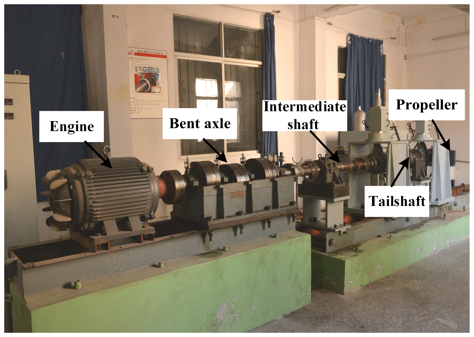
In this paper, the data sets of vibration signals for the bearing and propeller shaft are obtained based on the experimental platform of a ship propulsion shaft. The physical diagram is shown in Fig. 1. The total length of the shaft system of the test bench is 2665 mm. It consists of a drive shaft (driven by a variable frequency motor), a reducer, a thrust bearing with support, a propeller, a foundation, a base and a number of sensors. In addition, it is equipped with lubrication, hydraulic loading and condition-monitoring systems.
In the vibration test, the acquisition of bearing vibration signals is realised through a triaxial accelerometer sensor (Brüel & Kjær (B & K) 4535-B-001) located on the bearing seat, as shown in Fig. 2a. The vibration signals of the propeller shaft are obtained by a laser displacement sensor (Optex CD33-50NV), as shown in Fig. 2b. The multichannel signal analyser (signal acquisition; PXIE-4499) consists of servo amplifier, signal acquisition card and signal output device for data acquisition and vibration information acquisition. Thus, the vibration acceleration signal of the bearing and propeller shaft can be obtained simultaneously. The data set of the training neural network is designed to be 100 rpm (revolutions per minute). In order to test the network more accurately, the vibration response with rotational speeds of 150, 200, 250 and 300 rpm are selected as the test set.

2.2 Data collection and processing
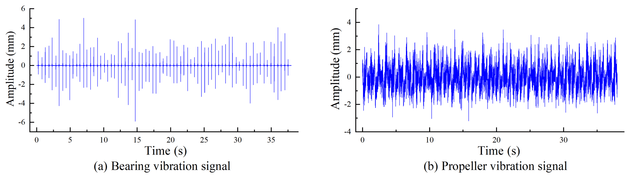
The data collection is mainly completed by the sensors, the acquisition module and the storage module. The triaxial acceleration sensor and displacement sensor convert the physical quantity into electrical signals, the acquisition module is responsible for converting the electrical signals of the sensor into digital signals, and the PC terminal is responsible for displaying and saving the strain data. Moreover, the LabVIEW measurement and control software are applied to visualise and record the data. The acceleration response of the bearing and the displacement response of the propeller shaft can be measured (as shown in Fig. 3).
In order to ensure that the vibration signal is not distorted as far as possible, a higher sampling frequency is selected. The sampling number N is 760 000, the sampling interval is 0.00005 s, and the sampling frequency is 20 000 Hz. It is difficult to deal with such a large volume of data in real time as the prediction of neural network is applied. Therefore, it is necessary to analyse the frequency of the collected signal and reselect the appropriate sampling frequency.
The vibration signals collected in the experiment are generally aperiodic discrete signals. For the transformation of discrete signals, only the discrete Fourier transform (DFT) method will be applied, and only the discrete and finite length data can be processed by the computer. The fast Fourier transform (FFT), as a fast algorithm of DFT, can greatly reduce the processing time of the timing signal. Figure 4 is the amplitude–frequency curve of the original signal after the FFT.
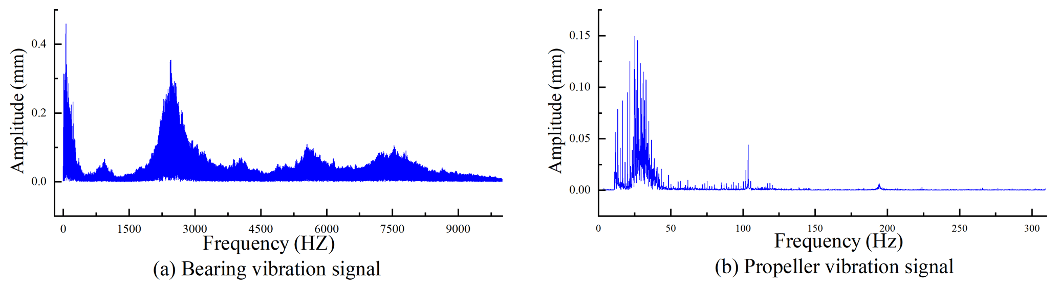
As can be seen from Fig. 4, the frequency of the vibration signals of the bearing are mainly concentrated within 2500 Hz. According to the sampling theorem, the sampling frequency is 2 times greater than the highest frequency of the signal. The frequency of the vibration sample is repositioned as 5000 Hz to avoid the distortion of the signal. Then, a frequency analysis of propeller shaft vibration is carried out, and the vibration frequency of the propeller shaft is mainly concentrated within 120 Hz, which determines the number of neurons in the output layer of the neural network.
3.1 Principles of the convolutional neural network
The convolutional neural network (CNN) is one of the most popular models among many neural network models (Abdel-Hamid et al., 2014). It can be traced back to the neocognitron proposed by Fukushima (1980), with continuous improvements by a large number of researchers, which has developed into current CNN. It is able to extract some abstract features efficiently and accurately because of its powerful feature extraction capability. The CNN model is originally a two-dimensional (2D) neural network with a 2D matrix as input. With the deepening of the research, it has been found that CNN also has a strong feature extraction ability for one-dimensional timing signals and has achieved good results in the vibration signal processing (Ma et al., 2020), fault diagnosis (Khan et al., 2018), natural language recognition (NLP; Zhao et al., 2018; Zhang et al., 2017) and other fields.
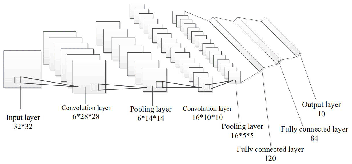
CNN is a kind of deep neural network with a convolutional structure, which can effectively reduce the parameters to be trained. The three most important core ideas of convolutional neural network are as follows: the local receptive field, weight sharing and pooling, which can greatly reduce the number of parameters and alleviate the overfitting problem of the model. Handwritten digit recognition is the most typical case applied by CNN, and its accuracy has been qualitatively improved compared with other traditional methods (Waibel et al., 1989). The convolutional neural network is mainly composed of an input layer, convolutional layer, pooling layer, full connection layer and output layer. The network structure of the classic CNN network LeNet (LeCun et al., 1998) is shown in Fig. 5.
The convolution layer is composed of several convolution kernels. Different from the traditional BP neural network, these convolution kernels are variable in length and width. Each convolution kernel has multiple learnable parameters which can be used for convolution operation to enhance the features of original information and reduce the interference of noise. The following is the mathematical model of convolution operation, as shown in the formula (Guo et al., 2019):
where is the jth feature map of the lth convolutional layer, and is the net activation of the jth channel on the jth convolutional layer. The calculation method is that each feature map of the previous layer is convolved by a learnable convolution kernel, then the overall sum is added with an offset, and finally the feature map is output through the activation function. is the convolution kernel, is the bias, and f(⋅) is the activation function.
The pooling layer, also known as the lower sampling layer, mainly conducts down-sampling processing on the original signal. It can effectively reduce the data volume, speed up the training and real-time processing capacity and avoid overfitting to a certain extent. Pooling is further divided into mean pooling and maximum pooling. The mean pooling is generally adopted in one-dimensional signal field, and maximum pooling is applied in two-dimensional signal field.
The core of training the neural network is to make the loss function decrease as the number of iterations increases, which is mainly realised by the gradient descent method. When the input passes through the neural network, the function of the sum will be obtained, which is the predicted value. The mean square deviation of the difference between actual value and predicted value is called the residual error. During the back propagation, the direction which reduces L can be obtained by taking the partial derivative of each learnable parameter and aiming at the update of trainable parameters. Meanwhile, an appropriate learning rate can be set to control the intensity of the residual back propagation. The updated formula of weight W and bias B is as follows (Li et al., 2021):
where Wi is the weight of the ith layer, η is the learning rate, E is the residual error, and bi is the bias of the ith layer.
3.2 The principle of a back-propagation neural network
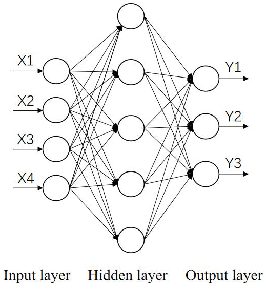
Back-propagation neural network (BPNN) is one of the most classic neural networks, which was proposed by Rumelhart and McClellandetal (1986). BPNN constantly train neurons in the network according to the error between the predicted value and the real value. This training method is called back propagation, which is also the core training method of neural network. The BP neural network mainly consists of an input layer, an output layer and a number of hidden layers. The learning process of a neural network can be mainly divided into two stages. In the first stage (also known as forward propagation), the input signal is transmitted layer by layer. For each neuron, there are two trainable parameters, and the output value is obtained after calculation. In the second stage (also known as back propagation), there is a deviation between the predicted value and the expected value; the partial derivative of each is taken in a recursive step-by-step manner, reducing the error in the direction of the smaller. The error will converge to a certain interval, and the network training will be completed after constant iteration. The multilayer feed-forward network structure, based on a BP neural network algorithm, is shown in Fig. 6 (Li et al., 2017). The mathematical model of this approach is as shown in the following:
The function f(x) is a simple sigmoid function, as follows:
Combining the formulas of Eqs. (5) and (6) can result in Eq. (7), as follows:
The weight update of the BP neural network reduces the error. The weight update of the formula is as follows:
where δ is the learning rate, E is the error between the network output and the expected output, and t is the number of network layers.
3.3 The principle of a recurrent neural network
A recurrent neural network (RNN) is a feed-forward neural network with a time connection. The information received by a neuron not only includes the output of the previous neuron but also includes its own state at the previous moment. It makes the RNN more advantageous in the processing of timing signals. Bidirectional RNN (Bi-RNN) is one of the most popular algorithms in deep learning (Elman, 1990) and is now in the Bi-RNN (Bi-RNN) field. The long short-term memory (LSTM) network, a recursive neural network (Schmidhuber, 2015), is an important branch of RNN, which has been widely used to process various time series signals. As in the field of predicting battery life, LSTM can achieve better performance (Jiao et al., 2021). The network structure of a RNN is shown in Fig. 7 (Guo et al., 2021).
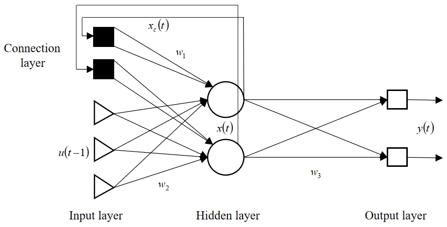
In RNN, the Elman (1990) network is connected between two cycle units, and the Jordan network is connected with a closed loop. The corresponding recursive mode is as follows (Pollack, 1990):
Elman (1990):
Jordan (Elman, 1990):
where f and g are activation functions, such as the sigmoid function and hyperbolic tangent function, t is time, and u and v are memory weights (trainable parameters).
3.4 Comparison and selection of models
The most suitable network model varies in different cases. Therefore, three popular models, CNN, BP and RNN, are compared. With the same quantity of the trainable parameters and 10 000 times of training, the prediction accuracy of the three models is obtained. The prediction results are shown in Fig. 8. At the same time, several model evaluation indexes are introduced to evaluate the performance of the model. The evaluation indexes of the regression model mainly include RMSE (root mean squared error), RAE (relative absolute error), MRE (mean relative error) and R2 (coefficient of determination). Its formula is shown as Eqs. (11)–(14) in the following:
Of these, Pi is the predicted target, and ai is the actual target. is the average of the true values. RMSE, RAE and MRE are error calculation formulas. The smaller the value, the better the performance of the model. R2 is between 0 and 1, and the closer it is to 1, the higher the accuracy of the model. According to the model evaluation indexes, the training results of each model are shown in Table 1.
Table 1Values of different models under different evaluation indexes.
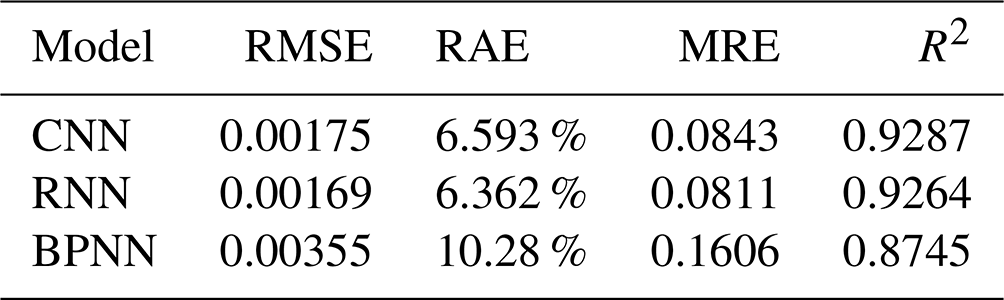

It can be seen from the table that when the number of trainable parameters is the same, the prediction accuracy of RNN is slightly higher than that of CNN, and both are higher than that of BPNN. However, the response speed of RNN is significantly lower than that of CNN because RNN needs to process vibration signals multiple different times at the same time in the prediction process, and the response speed is about 10 times slower than CNN, which depends on the model design of RNN. Considering that real-time monitoring requires a high response rate and a comprehensive prediction accuracy, CNN is finally selected for the following research.
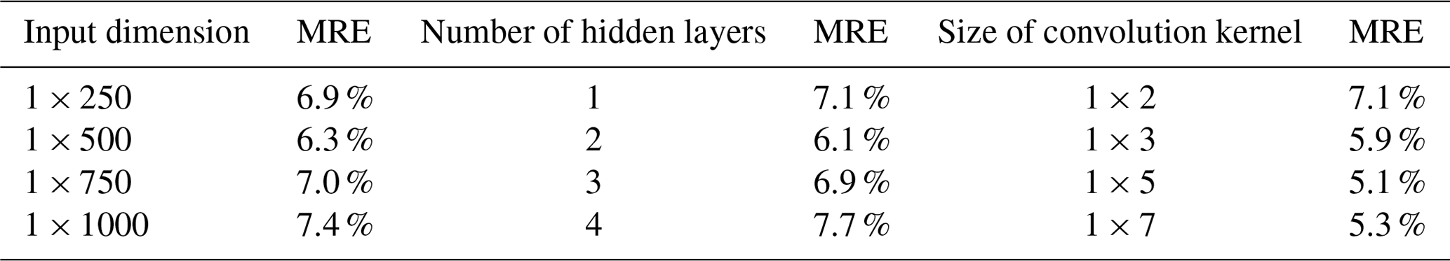
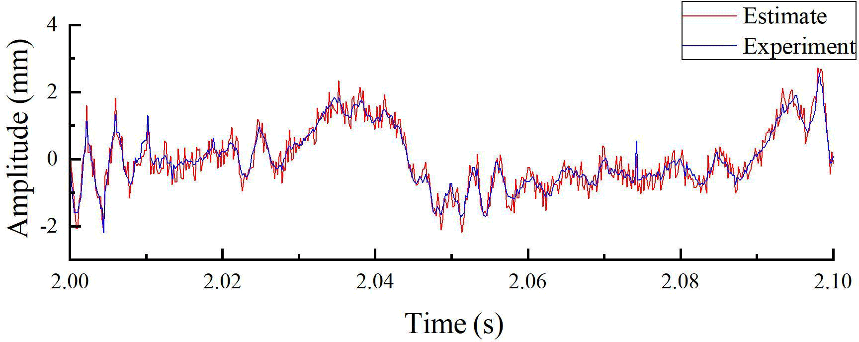
Table 3Errors in the time domain and frequency domain under different working conditions.

4.1 Selection of hyperparameters of neural networks
The selection of superparameters is very important as the neural network is building, which directly affects the performance of the network. Hyperparameters include the number of neurons per layer, the number of hidden layers and the size of the filter bank. Then, each parameter will be analysed, and the selection will be determined, as shown in Table 2.
-
The design of the input layer and output layer. The bearing vibration signals are generally non-periodic signals and can be considered as being composed of a multiple superposition of the periodic signal, which is the input of the neural network. The span of each input timing signal needs, as far as possible, to be large to ensure that it covers most of the bearing vibration cycle. Based on the frequency analysis in the previous study, the vector dimensions of different input layers and RAE after 1000 iterations are compared. Finally, the input layer is defined to be a 1×500 one-dimensional vector and 1×50 one-dimensional vector for the output layer.
-
The number of hidden layers. A deeper network structure will lead to overfitting, while a shallower network will lead to an inability to fit the nonlinear relationship between input and output effectively. In general, the two-layer fully connected layer is sufficient to meet the requirements of most problems. In the case of a large volume of data, the number of layers can be appropriately increased to achieve higher accuracy. Through comparing the number of different hidden layers, the mean absolute errors on the test set after an iteration of 1000 times can be determined, as shown in Table 2. Finally, it adopts two layers of a fully connected layer, and two sets of a CBAPD (convolution + batch normalisation + activation function + pooling + dropout) layer. Among them, the pooling layer adopts mean pooling, and the step size of the pooling is 2.
-
Size of the convolutional kernel. The convolutional kernel is the main learning parameter of the convolutional neural network. In order to improve the receptive field, the convolutional kernel with a value greater than 2 is generally adopted. After 1000 iterations, the mean absolute errors on the test set with different convolution kernel sizes were compared, as shown in Table 2. A 1×5 size convolution kernel is used, and the number of channels is three. At the same time, the full zero edge filling is adopted to keep the dimension unchanged when the input passes through the convolutional layer.
-
Activation functions. The rectified linear unit (ReLU) is the most popular activation function in the field of deep learning, which can effectively alleviate the problem of gradient disappearance and can also speed up the training speed of deep learning models. The expression of ReLU is as follows:
-
Loss function. For regression problems, the mean square error (MSE) is generally adopted as the loss function. The L2 regularisation term is also used to prevent overfitting. The principle is as follows:
where m is the number of samples, yi is the experimental result, is the predicted result, and w is the weight of neurons.
4.2 Training of convolutional neural network model
Through experiments, two sets of data are obtained under various working conditions. Each set of data contains the response of 760 000 results bearing the acceleration and shaft displacement. In total, 80 % of the 100 rpm data set is taken as the training set of the neural network and the rest 20 % as the test set. The data of 150 rpm are taken as the final test set to demonstrate the feasibility and universality of the proposed method. The prediction results can be seen in Fig. 9. It shows that the network fits well on the training set when the value of the RMSE in the training set is 0.00026 and the MRE is 3.37 %.
4.3 Test of convolutional neural network model
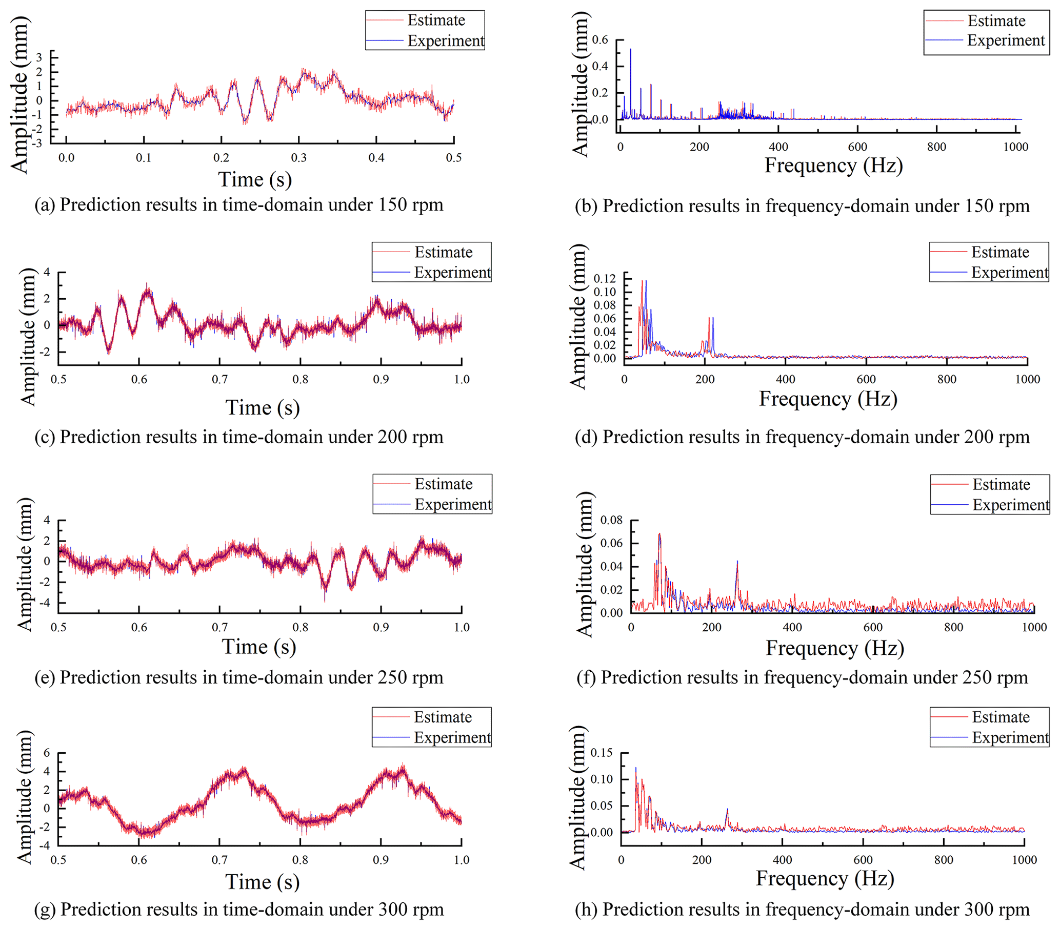
In order to guarantee the high prediction accuracy of the trained neural network under different working conditions, experimental data sets of various conditions are collected to demonstrate the feasibility of the method. About 5000 continuous vibration signals are taken as sample data for each condition and substituted into the neural network. The prediction results are displayed in Fig. 10a–h, with the MRE of each working condition shown in Table 3.
The results show that the trained convolutional neural network model has a better prediction accuracy in the time domain under different working conditions, with a prediction accuracy of more than 96 %. Meanwhile, in order to check the distortion of the predicted results in the frequency domain, the discrete Fourier transform (DFT), based on the experimental and predicted values, is conducted. The frequency components of the predicted results and the experimental values are compared. It shows that a high accuracy can still be maintained in the low-frequency part of the frequency domain. The high-frequency part of more than 400 Hz has a certain distortion and larger noise.
In this paper, a variety of neural network models are applied to predict the vibration signal of the marine propeller shaft. Through comparative analysis, it is found that RNN has certain advantages in the prediction accuracy when dealing with problems about timing signals, but this advantage is not obvious compared with CNN (see Table 2 and Fig. 8 for specific data). The reason may be that, although the vibration signal has a certain periodicity, the context is not as closely related as the sound signal, so this advantage cannot be effectively highlighted. In terms of the response rate, the RNN can not achieve an ideal effect, and the CNN is relatively balanced in the response rate and prediction accuracy.
The experimental results show that when the trainable parameters are the same, the prediction accuracy of the RNN is significantly higher than that of the BPNN. That means that the feature extraction ability of the convolution layer is significantly stronger than that of the full connection layer. When CNN is selected as the follow-up applied method through the optimisation and training of neural network, the feasibility is demonstrated in the test set, as its prediction accuracy is more than 90 %. And the prediction accuracy could be more than 95 % when only the low-frequency part is considered, which is also the t limitation of the proposed method. The signal of the high-frequency part shows a weak prediction accuracy, but this can be ignored for a low-speed rotational shaft such as a marine propeller shaft.
In this research, a reliable method to estimate the vibration response of a propeller shaft is proposed. Based on the convolutional neural network, the nonlinear relationship between the vibration signals of the bearing and propeller shaft is fitted. The dynamical response of the propeller shaft is predicted from the vibration signals of bearings that are experimentally measured. Compared with the traditional measurement method, the cost is lower, and the maintenance is simple for the proposed method. Moreover, this method is more suitable for the marine propeller shaft with a lower rotational speed.
With the verification based on the experimental data, the results show that the convolutional neural network can fit the nonlinear relationship between the vibration signals of a bearing and propeller shaft. It has high prediction accuracy in both the time and frequency domains. The low-frequency (less than 400 Hz) part can guarantee high accuracy. The distortion in the high-frequency part should be negligible for lower speed rotors, as the marine propeller shaft with the vibration frequency is mainly concentrated within 300 Hz.
All the code and data used in this paper can be obtained upon request to the corresponding author.
XS conceptualised the work, developed the methodology with QH, wrote the software, collected the resources and wrote and prepared the original draft with GX. QH led the review and editing of the paper and curated the data. All authors have read and agreed to the published version of the paper.
The contact author has declared that neither they nor their co-authors have any competing interests.
Publisher’s note: Copernicus Publications remains neutral with regard to jurisdictional claims in published maps and institutional affiliations.
The authors would like to thank the anonymous reviewers, for their valuable comments and suggestions that enabled us to revise the paper.
This research has been supported by the National Natural Science Foundation of China (grant nos. 51809201 and 51805383), the Key Laboratory of Marine Power Engineering and Technology (Wuhan University of Technology), the Ministry of Transport (grant no. KLMPET2018-05) and the National Engineering Research Center for Water Transport Safety (grant no. A2021005).
This paper was edited by Daniel Condurache and reviewed by Iosif Birlescu and three anonymous referees.
Abbas, S. H., Jang, J. K., Kim, D. H., and Lee, J.-R.: Underwater vibration analysis method for rotating propeller blades using laser Doppler vibrometer, Opt. Laser Eng., 132, 106133, https://doi.org/10.1016/j.optlaseng.2020.106133, 2020.
Abdel-Hamid, O., Mohamed, A., Jiang, H., Deng, L., Penn, G., and Yu, D.: Convolutional neural networks for speech recognition, IEEE-Acm. T. Audio Spe., 22, 1533–1545, https://doi.org/10.1109/TASLP.2014.2339736, 2014.
Al-Bedoor, B.: Dynamic model of coupled shaft torsional and blade bending deformations in rotors, Comput. Method. Appl. M., 169, 177–190, https://doi.org/10.1016/S0045-7825(98)00184-4, 1999.
Bauchau, O. and Hong, C.: Finite element approach to rotor blade modeling, J. Am. Helicopter Soc., 32, 60–67, https://doi.org/10.4050/JAHS.32.60, 1987.
Elman, J.: Finding structure in time, Cog. Sci., 14, 179–211, https://doi.org/10.1207/s15516709cog1402_1, 1990.
Fukushima, K.: Neocognitron: A self-organizing neural network model for a mechanism of pattern recognition unaffected by shift in position, Biol. Cybern., 36, 193–202, https://doi.org/10.1007/BF00344251, 1980.
Guo, Y., Zeng, Y.-c., Zeng, L.-c., Fu L.-d., and Zhan, C.-c.: Online Measurement of Hydraulic Cylinder Leakage Based on Neural Network, Chinese Hydraulics and Pneumatics, 09, 36–44, https://doi.org/10.11832/j.issn.1000-4858.2019.09.006, 2019.
Guo, Y., Xiong, G., Zeng, L., and Li, Q.: Modeling and Predictive Analysis of Small Internal Leakage of Hydraulic Cylinder Based on Neural Network, Energies, 14, 2456, https://doi.org/10.3390/en14092456, 2021.
He, J., Li, Y., Cao, J., Li, Y., Jiang, Y., and An, L.: An improved particle filter propeller fault prediction method based on grey prediction for underwater vehicles, T. I. Meas. Control., 42, 1946–1959, https://doi.org/10.1177/0142331219901202, 2020.
Jiao, M., Wang, D., Yang, Y., and Liu, F.: More intelligent and robust estimation of battery state-of-charge with an improved regularized extreme learning machine, Eng. Appl. Artif. Intel., 104, 104407, https://doi.org/10.1016/j.engappai.2021.104407, 2021.
Khan, M., Kim, Y., and Choo, J.: Intelligent fault detection using raw vibration signals via dilated convolutional neural networks, J. Supercomput., 76, 8086–8100, https://doi.org/10.1007/s11227-018-2711-0, 2018.
Kuantama, E., Moldovan, O., Ţarcă, I., Vesselényi, T., and Ţarcă, R.: Analysis of quadcopter propeller vibration based on laser vibrometer, J. Low Freq. Noise Vib., 40, 239–251, https://doi.org/10.1177/1461348419866292, 2021.
LeCun, Y., Bottou, L., Bengio, Y., and Haffner, P.: Gradient-based learning applied to document recognition, Proc. IEEE, 86, 2278–2324, https://doi.org/10.1109/5.726791, 1998.
Li, H., Yue, X., Wang, Z., Wang, W., Tomiyama, H., and Meng, L.: A survey of Convolutional Neural Networks – From software to hardware and the applications in measurement, Measurement Sensors, 18, 2508–2515, https://doi.org/10.1016/j.measen.2021.100080, 2021.
Li L., Tao, J.-f., Huang, Y.-x., and Liu, C.-l.: Internal Leakage Detection of Hydraulic Cylinder Based on BP Neural Network, Chinese Hydraulics and Pneumatics, 07, 11–15, https://doi.org/10.11832/j.issn.1000-4858.2017.07.003, 2017.
Ma, Y., Xisheng, J., Bai, H., Guo, C., and Wang, S.: Fault diagnosis of compressed vibration signal based on 1-dimensional CNN with optimized parameters, Systems Engineering and Electronics, 42, 1911–1919, https://doi.org/10.3969/j.issn.1001-506X.2020.09.05, 2020.
Morin, A., Arsenault, M., Edgecombe, M. H., and Radloff, E. A.: Real-time monitoring of ice-breaker propeller blades' ice load using underwater laser ranging system.Three-Dimensional Image Capture and Applications II, International Society for Optics and Photonics, 3640, 206–216, https://doi.org/10.1117/12.341062, 1999.
Ou, L.: Fault Diagnosis of Propeller Blade Breakdown Based on Vibration Method, Guangdong Shipbuilding, 38, 37–42, https://doi.org/10.3969/j.issn.2095-6622.2019.01.020, 2019.
Pollack, J. B.: Recursive distributed representations, Artificial Intelligence, 46, 77–105, https://doi.org/10.1016/0004-3702(90)90005-K, 1990.
Scalzo, A., Allen, J., and Antos, R.: Analysis and solution of a nonsynchronous vibration problem in the last row turbine blade of a large industrial combustion turbine, J. Eng. Gas. Turb. Power, 108, 591–598, https://doi.org/10.1115/86-GT-230, 1986.
Schmidhuber, J.: Deep learning in neural networks: An overview, Neural Networks, 61, 85–117, https://doi.org/10.1016/j.neunet.2014.09.003, 2015.
Srinivasan, A.: Vibrations of bladed-disk assemblies – A selected survey, J. Vib. Control, 106, 165–168, https://doi.org/10.1115/1.3269162, 1984.
Tang, D. and Dowell, E.: Experimental and theoretical study for nonlinear aeroelastic behavior of a flexible rotor blade, AIAA J., 31, 1133–1142, https://doi.org/10.2514/3.11738, 1993.
Waibel, A., Hanazawa, T., Hinton, G., Shikano, K., and Lang, K. J.: Phoneme recognition using time-delay neural networks, IEEE transactions on acoustics, speech, and signal processing, 37, 328–339, https://doi.org/10.1109/29.21701, 1989.
Zhang, X., Zou, Y., and Shi, W.: Dilated convolution neural network with LeakyReLU for environmental sound classification, 2017 22nd International Conference on Digital Signal Processing (DSP), IEEE, 1–5, https://doi.org/10.1109/ICDSP.2017.8096153, 2017.
Zhao, J., Mao, X., and Chen, L.: Learning deep features to recognise speech emotion using merged deep CNN. IET Signal Processing, 12, 713–721, https://doi.org/10.1049/iet-spr.2017.0320, 2018.
- Abstract
- Introduction
- Experimental environment and data processing
- The principle of neural network and the selection of network model
- Convolutional neural network model construction
- Discussion
- Conclusions
- Code and data availability
- Author contributions
- Competing interests
- Disclaimer
- Acknowledgements
- Financial support
- Review statement
- References