Constraint-following control design for the position tracking of a permanent magnet linear motor with inequality constraints

In this paper, we mainly solve the problem of the trajectory following the control and boundary transfinite control of the permanent magnet linear motor (PMLM). Using the Udwadia–Kalaba (U–K) method, the explicit equation of the complete nonholonomic constraint equation is first established, and then the new input constraint equation is obtained by integrating the inequality constraint and the original equation constraint through tangent-state transformation mapping. This constraint equation can make the motor move along the ideal trajectory in a limited range, thus solving the control problem of equality and inequality creatively. The simulation results and PMLM experiment results, based on control Signal Processing And Control Engineering (cSPACE), show that the proposed control method can obtain better motion performance, and the motion displacement does not exceed the boundary while satisfying the trajectory tracking control performance, which proves the effectiveness and feasibility of the proposed method.

1 Introduction

The linear motor is a kind of mechanical energy that can convert electrical energy directly into linear motion. This motor does not need any buffer device and can directly convert the input electrical signal into speed signal or position signal of linear motion. Therefore, linear motors with high speed and high precision have been applied to all kinds of machines and tools. For example, semiconductor manufacturing equipment and automatic testing equipment used in many factories are all equipped with this kind of motor (Huang et al., 2021).

The linear motor system has the characteristics of nonlinearity, multi-coupling, uncertainty, and so on. At the same time, due to the cancellation of the intermediate transmission device of the linear motor, the output of the motor is easily affected by various nonlinear factors, such as system end-effect and load disturbance. All these factors mentioned above increase the difficulty of electrical control of the linear motor (Eguren et al., 2020). In the current industrial application of the moving platform, proportion integration differentiation (PID) control is still the main control method of motor electrical control. However, because the traditional PID control is based on error elimination, it is difficult to meet the requirements of high-motion precision, fast speed, small overshoot, and strong anti-interference ability. There is still a lot of optimization space (Liu et al., 2020). Therefore, it is of great significance to study the control strategy of the linear motor.

In the past few decades, in addition to the industry, academia has also carried out a lot of research on linear motor motion control. In the control technology of permanent magnet linear motor (PMLM), precise control of linear motor displacement is essential. But some unknown external interference increases the difficulty of linear motor position control. Therefore, how to improve the control performance of PMLM has attracted a lot of attention in recent years, and many researchers have carried out in-depth research on this topic (Li et al., 2021). Early work includes an H-∞ optimal feedback control that provides high dynamic stiffness, as seen in Alter and Tsao (1996). The chaos system of permanent magnet linear synchronous motor is analyzed, and a new sliding mode composite chaos control strategy is proposed in Xie et al. (2019). Later, in order to suppress the force disturbance of PMLM, a feedforward neural network, based on the BP (backpropagation) algorithm, is proposed to approximate and compensate the force fluctuation, so as to achieve accurate motion control, as seen in Tan and Zhao (2004). In Krämer et al. (2022), the permanent magnet linear synchronous motors' high dynamic and energy-efficient operation is of interest. In particular, a new optimal force control strategy was developed and experimentally verified on a test bench.

After that, in order to further improve the precision of motion control, a lot of research work appeared. For example, in Chen et al. (2019), Liu et al. (2019), Huang et al. (2021), Yousefi et al. (2011), Wang et al. (2017), Liu et al. (2021), and Jafari et al. (2021) the fractional active disturbance rejection control strategy, optimal robust controller, input constrained nonlinear dynamics model, inequality state constraints, and control constraints and other schemes have been proposed successively. These schemes can achieve good tracking performance and anti-interference ability and have been widely applied in various industrial scenarios.

However, in the actual industrial scenarios, the control accuracy and stability of PMLM must be guaranteed, and the displacement must be limited to within a certain range in order to avoid the collision accident of PMLM under an external interference. Whether these limiting conditions can be satisfied is actually closely related to safe production. Therefore, in Meng et al. (2015), the author proposed to use the system transformation technology to transform the original constrained system into an equivalent unconstrained system which successfully solved the output constraint problem. In Duan and Li (2016), the author studied the modeling of a target motion under linear constraints. First, explicitly establish the linear equality constraints imposed by the line. Based on this, two constrained motion models are obtained by direct elimination and motion projection. By studying the relationship between the two models, the authors find that, for the first model, the conditions that guarantee the traditional linear Gaussian hypothesis can be obtained, while, for the second model, the conditions that the motion along each axis are similar to those along the trajectory can be obtained.

Recently, in Huang et al. (2020), the authors proposed a robust approximate constraint tracking control method for PMLM, based on the Udwadia–Kalaba (U–K) basic equation (Udwadia and Kalaba, 2002; Kalaba and Udwadia, 2001). There are two basic ideas in this method. One is to assume the control objectives (system stabilization, trajectory tracking, optimal control, etc.) of the system as a series of constraints. Second, the task of control is to drive the system to meet these constraints (Chen, 2009; Chen and Zhang, 2010; Zhao et al., 2018). However, most of the existing researchers do not consider the boundary constraints of PMSM, especially the problem of out-of-boundary motion control that may occur after the interference of external environment.

Inspired by the above research, a PMLM trajectory tracking control method with inequality constraints is proposed in our paper, which not only ensures the control accuracy and stability but also considers the uncertainties and unknown external disturbances of the system. From the perspective of engineering (such as control force, parameter setting, realizability, generality, etc.), the main contributions of this paper are as follows:

• i.

  Based on model and error, the proposed method inherits the characteristics of traditional U–K control, which can not only maintain the dynamic characteristics of the system but also achieve convergence. The strict proof of the Lyapunov minimax method is given, and the uniform boundedness and uniform ultimate boundedness of the controller are also proved in this paper.

• ii.

  The scheme presented in this paper can solve the system control problems with both equality and inequality constraints. By calling the reversible state transition, the inequality constraint of the state can be satisfied so that the actual state is bounded regardless of the uncertainty. This idea provides a general method to deal with inequality constraints for model-based control design.

• iii.

  The experimental results of the PMLM experiment platform based on control Signal Processing And Control Engineering (cSPACE) show that the proposed U–K equality constraint and inequality state transition method can obtain excellent system control performance with small precision loss. The proposed method has good performance and low control cost and can be extended to the safe control of other products.

2 System description and constraints

2.1 System description

The PMLM with uncertain parameters can be expressed as follows:

$$\begin{array}{}\text{(1)}& \begin{array}{rl}& \mathbf{M}\left(\mathit{\zeta }\right(t),\mathit{\sigma }(t),t)\ddot{\mathit{\zeta }}\left(t\right)+C\left(\mathit{\zeta }\right(t),\dot{\mathit{\zeta }}(t),\mathit{\sigma }(t),t)\\ & +\mathit{F}\left(\mathit{\zeta }\right(t),\mathit{\sigma }(t),t)=\mathit{\tau }\left(t\right),\end{array}\end{array}$$

where $t\in R\mathit{\zeta }\in R^n$ is the position with inequality constraints, $\dot{\mathit{\zeta }}\in R^n$ is the velocity, $\ddot{\mathit{\zeta }}\in R^n$ is the acceleration, and $\mathit{\sigma }\in \sum \subset R^P$ is the uncertain parameter (possibly time-varying). Here $\sum \subset R^P$ is compact but unknown, which stands for the possible bounding of σ. And τ is the control input. Furthermore, $\mathbf{M}\left(\mathit{\zeta },\mathit{\sigma },t\right)$ is the inertia matrix, $C\left(\mathit{\zeta },\dot{\mathit{\zeta }},\mathit{\sigma },t\right)$ is the Coriolis/centrifugal force, and $\mathit{F}\left(\mathit{\zeta },\mathit{\sigma },t\right)$ is the friction vector. One point needs to be emphasized, which is that the functions MCF are continuous in Eq. (1).

2.2 Equality constraints

In most practical circumstances, the motion of the system is constrained in some way. An equality constraint (i.e., bilateral constraint) is in the following form:

$$\begin{array}{}\text{(2)}& f_i(q,\dot{q},t)=\mathrm{0},i=\mathrm{1},\mathrm{2},\mathrm{\dots },m,\end{array}$$

where t∈R is the time, q∈Rⁿ is the position, and $\dot{q}$ is the velocity. The class of constraints, in the form of $f(q,\dot{q},t)=\mathrm{0}$, contains common types of holonomic and/or nonholonomic equality constraints.

Case 1: holonomic equality constraints

In general, according to the generalized coordinates selected, the description of the system will include u(u≤m) holonomic constraints. The holonomic equality constraints can be described as follows:

$$\begin{array}{}\text{(3)}& g_i(q,t)=\mathrm{0},i=\mathrm{1},\mathrm{2},\mathrm{\dots },u.\end{array}$$

Differentiating g_i(q,t) in Eq. (3), with respect to t, yields the following:

$$\begin{array}{}\text{(4)}& \sum _{j=\mathrm{1}}^n{\displaystyle \frac{\partial g_i(q,t)}{\partial q_j}}{\dot{q}}_j+{\displaystyle \frac{\partial g_i(q,t)}{\partial t}}=\mathrm{0}.\end{array}$$

The constraint (4) can be written in the following matrix form:

$$\begin{array}{}\text{(5)}& A(q,t)\dot{q}=b(q,t),\end{array}$$

where $A={\left[\frac{\partial g_i\left(q,t\right)}{\partial q_j}\right]}_{m\times n}b={\left[b_{\mathrm{1}},b_{\mathrm{2}},\mathrm{\dots },b_{\mathrm{m}}\right]}^{\mathrm{T}}$.

Case 2: nonholonomic equality constraints

And the r(r≤m) nonholonomic constraints form can be described as follows:

$$\begin{array}{}\text{(6)}& {\mathrm{\Phi }}_i(q,\dot{q},t)=\mathrm{0},i=\mathrm{1},\mathrm{2},\mathrm{\dots },r.\end{array}$$

The following constraint is considered:

$$\begin{array}{}\text{(7)}& \sum _{i=\mathrm{1}}^n{B}_i(q,t)\dot{q}+d_i(q,t)=\mathrm{0},i=\mathrm{1},\mathrm{2},\mathrm{\dots },r.\end{array}$$

Continuing to calculate the derivative of the constraint's second-order form with respect to t gives the following:

$$\begin{array}{}\text{(8)}& \begin{array}{rl}& \sum _{j=\mathrm{1}}^n{B}_{ij}(q,t){\ddot{q}}_j+\sum _{j=\mathrm{1}}^n\sum _{k=\mathrm{1}}^n{\displaystyle \frac{\partial B_{ij}(q,t)}{\partial q_k}}{\dot{q}}_k{\dot{q}}_j\\ & +\sum _{j=\mathrm{1}}^n{\displaystyle \frac{\partial B_{ij}(q,t)}{\partial t}}{\dot{q}}_j+\sum _{k=\mathrm{1}}^n{\displaystyle \frac{\partial d_i(q,t)}{\partial q_k}}{\dot{q}}_k\\ & +{\displaystyle \frac{\partial d_i(q,t)}{\partial t}}=\mathrm{0}.\end{array}\end{array}$$

Moreover, these constraints are all assumed to be smooth enough so that they are of sufficient differentiability with respect to time t to be transformed into their second-order form in Eq. (9) as follows:

$$\begin{array}{}\text{(9)}& A(q,\dot{q},t)\ddot{q}=c(q,\dot{q},t),\end{array}$$

where $A\in R_{m\times n}$ is termed as the constraint matrix, and $c={\left[c_{\mathrm{1}},c_{\mathrm{2}},\mathrm{\dots },c_{\mathrm{m}}\right]}^{\mathrm{T}}$. Chen (1999, 1998) shows how to calculate the constraint force when the uncertainty is known.

Because of the presence of constraints, the system should be subjected to extra generalized constraint forces. Thus, the actual explicit equation of the motion of the constrained system could be expressed as follows:

$$\begin{array}{}\text{(10)}& M(q,t)\ddot{q}=\mathbf{Q}(q,\dot{q},t)+{\mathbf{Q}}^{\mathrm{c}}(q,\dot{q},t),\end{array}$$

where ${\mathbf{Q}}^{\mathrm{c}}(q,\dot{q},t)$ is the constraint force matrix that guides the system to satisfy the restrictions. The work done by the constraint force Q^c under virtual displacement is zero, according to D'Alembert's principle (Udwadia and Kalaba, 2000; Udwadia, 2005). As a result, Q^c may be defined as follows:

$$\begin{array}{}\text{(11)}& Q^{\mathrm{c}}=M^{\mathrm{1}/\mathrm{2}}{B}^{+}(c-A{M}^{-\mathrm{1}}Q),\end{array}$$

where $B=A{M}^{-\frac{\mathrm{1}}{\mathrm{2}}}$, and the superscript + indicates the Moore–Penrose generalized inverse. Consequently, the explicit motion equation of constrained system can be written as follows:

$$\begin{array}{}\text{(12)}& M\ddot{q}=Q+M^{\mathrm{1}/\mathrm{2}}{B}^{+}(c-A{M}^{-\mathrm{1}}Q).\end{array}$$

Remark 1

A number of common constraints are included in the second-order form of constraint Eq. (9), including the holonomic constraint, nonholonomic constraint, scleronomic constraint, rheonomic constraint, and so on. The system's motion is altered by the combined action of the primary force and the binding force.

2.3 Inequality constraints

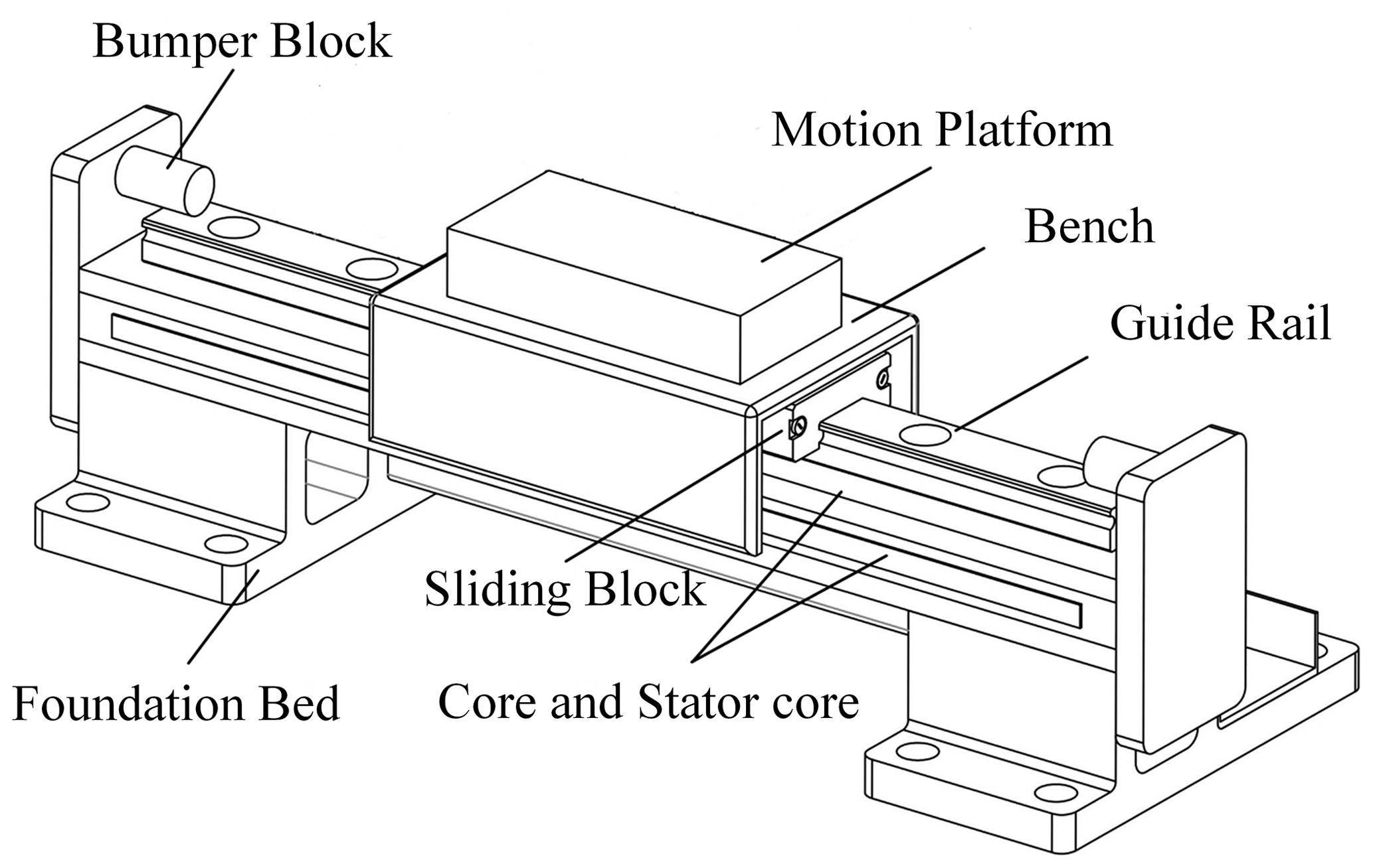
We consider the uncertain parameters that PMLM has to move in the limit range, such as the mass displacement of the moving platform, the dynamic displacement of the foundation bed, and the guide rail deflection, as shown in Fig. 1. Therefore, it is necessary to consider inequality constraints to prevent uncertainties from bumping into the bumper block, which can be written as a dual inequality constraint, as follows:

$$\begin{array}{}\text{(13)}& l_{\mathrm{m}}<{\mathit{\phi }}_i(q,t)<l_{\mathrm{M}},i=\mathrm{1},\mathrm{2},\mathrm{3}\mathrm{\dots },k,\end{array}$$

where l_m, l_M are constants.

Figure 1 Permanent magnet linear motor structure diagram.

Suppose that ${\mathit{\phi }}_i\left(q,t\right)\to {\mathit{\phi }}_{\mathrm{d}}\left(q,t\right)$ as $t\to +\mathrm{\infty }$, and the inequality constraint is $l_{\mathrm{m}}<{\mathit{\phi }}_i(q,t)<l_{\mathrm{M}}$, where φ_d(q,t) is the desired value of φ, l_m, and l_M are the maximum and minimum of φ, respectively.

Then, we can choose a proper transformation function for φ as Eq. (14) as follows:

$$\begin{array}{}\text{(14)}& {\mathit{\zeta }}_i=I\left({\mathit{\phi }}_i\right),i=\mathrm{1},\mathrm{2},\mathrm{3}\mathrm{\dots },k.\end{array}$$

The state of φ can be transformed to a new state ζ without any limitation. The function ζ=I(φ) should satisfy the condition that $\mathit{\zeta }\in \left(-\mathrm{\infty },+\mathrm{\infty }\right)$ as $\mathit{\phi }\in \left(l_{\mathrm{m}},l_{\mathrm{M}}\right)$. Since ζ_i=I(φ_i), we have the following:

$$\begin{array}{}\text{(15)}& {\mathit{\phi }}_i=I^{-\mathrm{1}}\left({\mathit{\zeta }}_i\right).\end{array}$$

Apparently, the tangent function is a map that can be used to construct a diffeomorphism for Eq. (15). Therefore, the following diffeomorphisms are selected for φ, where, in the following:

$$\begin{array}{}\text{(16)}& {\displaystyle }{\mathit{\zeta }}_i=I\left({\mathit{\phi }}_i\right)=\tan \left({\displaystyle \frac{l_i-l_{\mathrm{m}}}{l_{\mathrm{M}}-l_{\mathrm{m}}}}\mathit{\pi }-{\displaystyle \frac{\mathit{\pi }}{\mathrm{2}}}\right)\text{(17)}& {\displaystyle }{\mathit{\zeta }}_{\mathrm{d}}=I\left({\mathit{\phi }}_{\mathrm{d}}\right)=\tan \left({\displaystyle \frac{l_{\mathrm{d}}-l_{\mathrm{m}}}{l_{\mathrm{M}}-l_{\mathrm{m}}}}\mathit{\pi }-{\displaystyle \frac{\mathit{\pi }}{\mathrm{2}}}\right).\end{array}$$

This means that, in the following:

$$\begin{array}{}\text{(18)}& {\displaystyle }{\mathit{\phi }}_i=I^{-\mathrm{1}}\left({\mathit{\zeta }}_i\right)={\displaystyle \frac{l_{\mathrm{M}}-l_{\mathrm{m}}}{\mathit{\pi }}}\arctan {\mathit{\zeta }}_i+{\displaystyle \frac{l_{\mathrm{M}}+l_{\mathrm{m}}}{\mathrm{2}}}\text{(19)}& {\displaystyle }{\mathit{\phi }}_{\mathrm{d}}=I^{-\mathrm{1}}\left({\mathit{\zeta }}_{\mathrm{d}}\right)={\displaystyle \frac{l_{\mathrm{M}}-l_{\mathrm{m}}}{\mathit{\pi }}}\arctan {\mathit{\zeta }}_{\mathrm{d}}+{\displaystyle \frac{l_{\mathrm{M}}+l_{\mathrm{m}}}{\mathrm{2}}}.\end{array}$$

In this section, the state variable domain is transformed based on state transformation so that it can satisfy the inequality constraints of controlled outputs.

Remark 2

In this study, the inequality constraints of PMLM must be satisfied at any given time. On the contrary, the equality constraints shown in Eq. (9) may not be satisfied at some given time (e.g., the initial time) but only ensure that the motion of PMLM converges to the equality constraints.

3 Control design incorporating inequality constraints

3.1 Control design

Since the number of the items in $\widehat{I}:=[{\mathit{\zeta }}_{\mathrm{1}}{\mathit{\zeta }}_{\mathrm{2}},\mathrm{\dots }{\mathit{\zeta }}_k{]}^{\mathrm{T}}$ may be smaller than that of the items in q (i.e., k≤n), we need to introduce (n−l) additional variables so that the items in q can be expressed as explicit functions of Eq. (9). Let $\stackrel{\mathrm{̃}}{\mathit{I}}:=[{\mathit{\zeta }}_{k+\mathrm{1}}{\mathit{\zeta }}_{k+\mathrm{2}},\mathrm{\dots }{\mathit{\zeta }}_n{]}^{\mathrm{T}}$, and the vector $\widehat{\mathit{I}}$ and $\stackrel{\mathrm{̃}}{\mathit{I}}$ constitute the vector $\mathit{I}=[\widehat{\mathit{I}}\stackrel{\mathrm{̃}}{\mathit{I}}{]}^{\mathrm{T}}$, which is a set of independent variables. The set $\stackrel{\mathrm{̃}}{\mathit{I}}$ may be related to the diffeomorphisms and contains the inequality constraints for state transitions, and ${\mathit{\zeta }}_i\left(i=k+\mathrm{1},k+\mathrm{2}\mathrm{\dots }n\right)$ are functions of items in q. By this, we may have the following relation between q and ζ:

$$\begin{array}{}\text{(20)}& q=h(\mathit{\zeta },t),\end{array}$$

where $h\left(\cdot \right):R^n\times R\to R^n$ can be derived according to the diffeomorphisms in Eq. (16) and the choice of $\stackrel{\mathrm{̃}}{\mathit{I}}$. Differentiating Eq. (20) with respect to t yields the following:

$$\begin{array}{}\text{(21)}& \dot{q}={\displaystyle \frac{\partial h(\mathit{\zeta },t)}{\partial \mathit{\zeta }}}\dot{\mathit{\zeta }}+{\displaystyle \frac{\partial h(\mathit{\zeta },t)}{\partial t}}.\end{array}$$

Next, by differentiating Eq. (21) with respect to t, we can obtain the following:

$$\begin{array}{}\text{(22)}& \ddot{q}={\displaystyle \frac{\partial h(\mathit{\zeta },t)}{\partial \mathit{\zeta }}}\ddot{\mathit{\zeta }}+{\displaystyle \frac{{\partial }^{\mathrm{2}}h(\mathit{\zeta },t)}{\partial {\mathit{\zeta }}^{\mathrm{2}}}}+\mathrm{2}{\displaystyle \frac{{\partial }^{\mathrm{2}}h(\mathit{\zeta },t)}{\partial \mathit{\zeta }\partial t}}\dot{\mathit{\zeta }}+{\displaystyle \frac{{\partial }^{\mathrm{2}}h(\mathit{\zeta },t)}{\partial t^{\mathrm{2}}}}.\end{array}$$

Substituting Eqs. (20)–(22) into the constraint in Eq. (9) yields the following:

$$\begin{array}{}\text{(23)}& \stackrel{\mathrm{̃}}{A}(\mathit{\zeta },\dot{\mathit{\zeta }},t)\ddot{\mathit{\zeta }}=\stackrel{\mathrm{̃}}{c}(\mathit{\zeta },\dot{\mathit{\zeta }},t),\end{array}$$

where, in the following:

$$\begin{array}{}\text{(24)}& \begin{array}{rl}& \stackrel{\mathrm{̃}}{A}=A{\displaystyle \frac{\partial h(\mathit{\zeta },t)}{\partial \mathit{\zeta }}}\\ & \stackrel{\mathrm{̃}}{c}=c-A\left({\displaystyle \frac{{\partial }^{\mathrm{2}}h(\mathit{\zeta },t)}{\partial {\mathit{\zeta }}^{\mathrm{2}}}}+\mathrm{2}{\displaystyle \frac{{\partial }^{\mathrm{2}}h(\mathit{\zeta },t)}{\partial \mathit{\zeta }\partial t}}\dot{F}+{\displaystyle \frac{{\partial }^{\mathrm{2}}h(\mathit{\zeta },t)}{\partial t^{\mathrm{2}}}}\right).\end{array}\end{array}$$

The constraint in Eq. (23) is consistent since the constraint in Eq. (9) is consistent. By substituting Eqs. (20)–(22) into Eq. (10), we yield the dynamic equation in the space of ζ.

$$\begin{array}{}\text{(25)}& \stackrel{\mathrm{̃}}{M}(\mathit{\zeta },t)\ddot{\mathit{\zeta }}=\stackrel{\mathrm{̃}}{Q}(\mathit{\zeta },\dot{\mathit{\zeta }},t)+{\stackrel{\mathrm{̃}}{Q}}^{\mathrm{c}}(\mathit{\zeta },\dot{\mathit{\zeta }},t),\end{array}$$

where, in the following:

$$\begin{array}{}\text{(26)}& \begin{array}{rl}& \stackrel{\mathrm{̃}}{M}=M{\displaystyle \frac{\partial h(\mathit{\zeta },t)}{\partial \mathit{\zeta }}},{\stackrel{\mathrm{̃}}{Q}}^{\mathrm{c}}=Q^{\mathrm{c}}\\ & \stackrel{\mathrm{̃}}{Q}=Q-M\left({\displaystyle \frac{{\partial }^{\mathrm{2}}h(\mathit{\zeta },t)}{\partial {\mathit{\zeta }}^{\mathrm{2}}}}+\mathrm{2}{\displaystyle \frac{{\partial }^{\mathrm{2}}h(\mathit{\zeta },t)}{\partial \mathit{\zeta }\partial t}}\dot{\mathit{\zeta }}+{\displaystyle \frac{{\partial }^{\mathrm{2}}h(\mathit{\zeta },t)}{\partial t^{\mathrm{2}}}}\right).\end{array}\end{array}$$

Accordingly, by the U–K approach and the diffeomorphisms, we can obtain the constraint force accounting for both equality and inequality constraints as follows:

$$\begin{array}{}\text{(27)}& Q^{\mathrm{c}}={\stackrel{\mathrm{̃}}{Q}}^{\mathrm{c}}={\stackrel{\mathrm{̃}}{M}}^{\mathrm{1}/\mathrm{2}}{\stackrel{\mathrm{̃}}{B}}^{+}(\stackrel{\mathrm{̃}}{c}-\stackrel{\mathrm{̃}}{A}{\stackrel{\mathrm{̃}}{M}}^{-\mathrm{1}}Q),\end{array}$$

where $\stackrel{\mathrm{̃}}{B}=\stackrel{\mathrm{̃}}{A}{\stackrel{\mathrm{̃}}{M}}^{-\frac{\mathrm{1}}{\mathrm{2}}}$.

Assumption 1

For each $(\mathit{\zeta },t)\in R^n\times R,\mathit{\sigma }\in \sum ,M(\mathit{\zeta },\mathit{\sigma },t)>\mathrm{0}$.

Assumption 2

The uncertain parameter $\mathit{\sigma }\in \sum$ is known.

The constraint force that satisfies Gauss's principle and Lagrange's form of D'Alembert's principle is explicitly supplied, based on the U–K equation and two aforementioned above.

$$\begin{array}{}\text{(28)}& \begin{array}{rl}& Q_s^{\mathrm{c}}(\mathit{\zeta },\dot{F},t)={\stackrel{\mathrm{‾}}{\stackrel{\mathrm{̃}}{M}}}^{\mathrm{1}/\mathrm{2}}(\mathit{\zeta },\mathit{\sigma },t){\left(\stackrel{\mathrm{̃}}{A}(\mathit{\zeta },t){\stackrel{\mathrm{‾}}{\stackrel{\mathrm{̃}}{M}}}^{-\mathrm{1}/\mathrm{2}}(\mathit{\zeta },\mathit{\sigma },t)\right)}^{+}\\ & \times \mathit{\left\{}\stackrel{\mathrm{̃}}{c}\right(\mathit{\zeta },\dot{\mathit{\zeta }},t)-\stackrel{\mathrm{̃}}{A}(\mathit{\zeta },t\left){\stackrel{\mathrm{‾}}{\stackrel{\mathrm{̃}}{M}}}^{-\mathrm{1}}\right(\mathit{\zeta },\mathit{\sigma },t)\\ & \times \left[\stackrel{\mathrm{‾}}{\stackrel{\mathrm{̃}}{C}}(\mathit{\zeta },\dot{\mathit{\zeta }},\mathit{\sigma },t)\dot{\mathit{\zeta }}+\stackrel{\mathrm{‾}}{\stackrel{\mathrm{̃}}{F}}(\mathit{\zeta },\mathit{\sigma },t)\right]\mathit{\}}.\end{array}\end{array}$$

Supposed that the variables M, C, and F in Eqs. (1) and (28) can be decomposed into the following:

$$\begin{array}{}\text{(29)}& \begin{array}{rl}& M(\mathit{\zeta },\mathit{\sigma },t)=\stackrel{\mathrm{‾}}{\stackrel{\mathrm{̃}}{M}}(\mathit{\zeta },t)+\mathrm{\Delta }M(\mathit{\zeta },\mathit{\sigma },t)\\ & C(\mathit{\zeta },\dot{\mathit{\zeta }},\mathit{\sigma },t)=\stackrel{\mathrm{‾}}{\stackrel{\mathrm{̃}}{C}}(\mathit{\zeta },\dot{\mathit{\zeta }},t)+\mathrm{\Delta }C(\mathit{\zeta },\dot{\mathit{\zeta }},\mathit{\sigma },t)\\ & F(\mathit{\zeta },\mathit{\sigma },t)=\stackrel{\mathrm{‾}}{\stackrel{\mathrm{̃}}{F}}(\mathit{\zeta },t)+\mathrm{\Delta }F(\mathit{\zeta },\mathit{\sigma },t),\end{array}\end{array}$$

where M, C, and F indicate the nominal portions, and ΔM, ΔC, and ΔF represent the uncertain portions in the constraint system. In order to simplify the controller design, let the following apply:

$$\begin{array}{}\text{(30)}& \begin{array}{rl}& H(\mathit{\zeta },t)={\stackrel{\mathrm{‾}}{\stackrel{\mathrm{̃}}{M}}}^{-\mathrm{1}}(\mathit{\zeta },t)\\ & \mathrm{\Delta }H(\mathit{\zeta },\mathit{\sigma },t)=M^{-\mathrm{1}}(\mathit{\zeta },\mathit{\sigma },t)-{\stackrel{\mathrm{‾}}{\stackrel{\mathrm{̃}}{M}}}^{-\mathrm{1}}(\mathit{\zeta },t)\\ & \mathrm{\Pi }(\mathit{\zeta },\mathit{\sigma },t)=\stackrel{\mathrm{‾}}{\stackrel{\mathrm{̃}}{M}}(\mathit{\zeta },t)M^{-\mathrm{1}}(\mathit{\zeta },\mathit{\sigma },t)-I.\end{array}\end{array}$$

According to formula (30), we can obtain $\mathrm{\Delta }\mathrm{\Pi }\left(\mathit{\zeta },\mathit{\sigma },t\right)=H(\mathit{\zeta },t)\mathrm{\Pi }\left(\mathit{\zeta },\mathit{\sigma },t\right)$.

Assumption 3

For any $\left(\mathit{\zeta },t\right)\in R^n\times R$ with inequality constraints, if A(ζ,t) is full rank, then it can be inverted.

Assumption 4

There is a constant ${\mathit{\rho }}_{\mathrm{\Pi }}>-\mathrm{1}$ such that $\left(\mathit{\zeta },t\right)\in R^n\times R$ satisfies the following:

$$\begin{array}{}\text{(31)}& {\displaystyle \frac{\mathrm{1}}{\mathrm{2}}}\underset{\mathit{\sigma }\in \sum }{min}{\mathit{\lambda }}_{\mathrm{m}}\left[\mathrm{\Pi }\right(\mathit{\zeta },\mathit{\sigma },t)+{\mathrm{\Pi }}^{\mathrm{T}}(\mathit{\zeta },\mathit{\sigma },t\left)\right]\ge {\mathit{\rho }}_{\mathrm{\Pi }}.\end{array}$$

The constant ρ_Π is usually unknown because the uncertain boundary is unknown. In special cases, if there is no uncertainty, then let $M=\stackrel{\mathrm{‾}}{\stackrel{\mathrm{̃}}{M}}$ (no uncertainty) and Π=0. Finally, ρ_Π=0 is optional.

Assumption 5

Based on the provision of Assumption 3, for a given $P\in R^{m\times m}P>\mathrm{0}$, let the following apply:

$$\begin{array}{}\text{(32)}& \mathrm{\Xi }(\mathit{\zeta },t):=PA(\mathit{\zeta },t)H(\mathit{\zeta },t)H(\mathit{\zeta },t)A^{\mathrm{T}}(\mathit{\zeta },t)P.\end{array}$$

There is a constant $\underset{\mathrm{¯}}{\mathit{\lambda }}>\mathrm{0}$, let the following apply:

$$\begin{array}{}\text{(33)}& \underset{(F,t)\in R^n\times R}{\inf }{\mathit{\lambda }}_{\mathrm{m}}\left[\mathrm{\Xi }\right(\mathit{\zeta },t\left)\right]\ge \underset{\mathrm{¯}}{\mathit{\lambda }}.\end{array}$$

The matrix Ξ(ζ,t) is uniformly positive definite, so the lower bound of its smallest eigenvalue is positive.

Based on Assumptions 1 and 2 and 3–5, a robust controller based on the U–K equation is given as follows:

$$\begin{array}{}\text{(34)}& \mathit{\tau }\left(t\right)=p_{\mathrm{1}}(\mathit{\zeta },\dot{\mathit{\zeta }},t)+p_{\mathrm{2}}(\mathit{\zeta },\dot{\mathit{\zeta }},t)+p_{\mathrm{3}}(\mathit{\zeta },\dot{\mathit{\zeta }},t),\end{array}$$

with the following:

$$\begin{array}{}\text{(35)}& \begin{array}{rl}& p_{\mathrm{1}}(\mathit{\zeta },\dot{\mathit{\zeta }},t)=Q_s^{\mathrm{c}}\\ & p_{\mathrm{2}}(\mathit{\zeta },\dot{\mathit{\zeta }},t)=-\mathit{\kappa }{\stackrel{\mathrm{‾}}{\stackrel{\mathrm{̃}}{M}}}^{-\mathrm{1}}(\mathit{\zeta },t){\stackrel{\mathrm{̃}}{A}}^{\mathrm{T}}(\mathit{\zeta },t)P\mathit{\beta }(\mathit{\zeta },\dot{\mathit{\zeta }},t)\\ & p_{\mathrm{3}}(\mathit{\zeta },\dot{\mathit{\zeta }},t)=-\mathit{\gamma }(\mathit{\zeta },\dot{\mathit{\zeta }},t)\mathit{\mu }(\mathit{\zeta },\dot{\mathit{\zeta }},t)\mathit{\rho }(\mathit{\zeta },\dot{\mathit{\zeta }},t),\end{array}\end{array}$$

where p₁ is the calculated ideal binding force. In the case of certainty, p₂ can make the control system stable and convergent, and p₃ is the ideal trajectory correction in the case of uncertainty. Here, κ>0, the function $\mathit{\gamma }\left(\mathit{\zeta },\dot{\mathit{\zeta }},t\right)$ is the adaptive control law which can be written as follows:

$$\begin{array}{}\text{(36)}& {\displaystyle }\mathit{\gamma }(\mathit{\zeta },\dot{\mathit{\zeta }},t)=\left\{\begin{array}{ll}\frac{[\mathrm{1}+{\mathit{\rho }}_{\mathrm{\Pi }}(\mathit{\zeta },\dot{\mathit{\zeta }},t){]}^{-\mathrm{1}}}{∥\mathit{\mu }(\mathit{\zeta },\dot{\mathit{\zeta }},t)∥}& ∥\mathit{\mu }(\mathit{\zeta },\dot{\mathit{\zeta }},t)∥>\mathit{\epsilon }\\ \frac{[\mathrm{1}+{\mathit{\rho }}_{\mathrm{\Pi }}(\mathit{\zeta },\dot{\mathit{\zeta }},t){]}^{-\mathrm{1}}}{\mathit{\epsilon }}& ∥\mathit{\mu }(\mathit{\zeta },\dot{\mathit{\zeta }},t)∥\le \mathit{\epsilon }\end{array}\right.\text{(37)}& {\displaystyle }\begin{array}{rl}& \mathit{\beta }(\mathit{\zeta },\dot{\mathit{\zeta }},t)=\stackrel{\mathrm{̃}}{A}(\mathit{\zeta },t)\dot{F}-c(\mathit{\zeta },t)\\ & \mathit{\mu }(\mathit{\zeta },\dot{\mathit{\zeta }},t)=\mathit{\eta }(\mathit{\zeta },\dot{\mathit{\zeta }},t)\mathit{\rho }(\mathit{\zeta },\dot{\mathit{\zeta }},t)\\ & \mathit{\eta }(\mathit{\zeta },\dot{\mathit{\zeta }},t)=\stackrel{\mathrm{‾}}{\mathit{\mu }}(\mathit{\zeta },\dot{\mathit{\zeta }},t)\mathit{\beta }(\mathit{\zeta },\dot{\mathit{\zeta }},t)\\ & \stackrel{\mathrm{‾}}{\mathit{\mu }}(\mathit{\zeta },\dot{\mathit{\zeta }},t)=H(\mathit{\zeta },t)A^{\mathrm{T}}(\mathit{\zeta },t)P.\end{array}\end{array}$$

The function ρ(⋅) is chosen such that, in the following:

$$\begin{array}{}\text{(38)}& \begin{array}{rl}& \mathit{\rho }(\mathit{\zeta },\dot{\mathit{\zeta }},t)\ge \underset{\mathit{\sigma }\in \sum }{min}\Vert P\stackrel{\mathrm{̃}}{A}\left[\mathrm{\Delta }H\right(-C\dot{\mathit{\zeta }}-F+p_{\mathrm{1}}+p_{\mathrm{2}})\\ & +H(-\mathrm{\Delta }C\mathit{\zeta }-\mathrm{\Delta }F)]\Vert .\end{array}\end{array}$$

By choosing suitable parameters κ and ε, the system input moment τ can be obtained according to Eqs. (34)–(38). Besides, under the action of the moment τ, β can satisfy consistent boundedness and consistent final boundedness.

3.2 Controller stability analysis

Theorem 1

Subject to Assumptions 1–5, consider the mechanical system incorporating inequality constraints. The control design renders the error β.

(i) Uniformly bounded

For any r>0, there is a d(r)<∞, such that if ∥β(t₀)∥≤r, then ∥β((t))∥≤d(r) for all t≥t₀.

(ii) Uniformly and ultimately bounded

For any r>0 with ∥β(t₀)∥≤r, there exists a $\underset{\mathrm{¯}}{d}>\mathrm{0}$, such that ∥β(t)∥≤d(r) for any $\stackrel{\mathrm{‾}}{d}>\underset{\mathrm{¯}}{d}$.

Proof

The candidate for the Lyapunov function is provided.

$$\begin{array}{}\text{(39)}& V\left(\mathit{\beta }\right)={\mathit{\beta }}^{\mathrm{T}}P\mathit{\beta }.\end{array}$$

For the corresponding β and uncertainty σ(t) expected by the control system, the first-order derivative of V(β) is expressed as follows:

$$\begin{array}{}\text{(40)}& \begin{array}{rl}\dot{V}& =\mathrm{2}{\mathit{\beta }}^{\mathrm{T}}P\dot{\mathit{\beta }}=\mathrm{2}{\mathit{\beta }}^{\mathrm{T}}P(\stackrel{\mathrm{̃}}{A}\ddot{\mathit{\zeta }}-\stackrel{\mathrm{̃}}{c})\\ & =\mathrm{2}{\mathit{\beta }}^{\mathrm{T}}P\mathit{\left\{}\stackrel{\mathrm{̃}}{A}\right[M^{-\mathrm{1}}(-C\dot{\mathit{\zeta }}-F)\\ & +M^{-\mathrm{1}}(p_{\mathrm{1}}+p_{\mathrm{2}}+p_{\mathrm{3}})]-\stackrel{\mathrm{̃}}{c}\mathit{\}}.\end{array}\end{array}$$

Substituting Eq. (30) into Eq. (40), we obtain the following:

$$\begin{array}{}\text{(41)}& \begin{array}{rl}\dot{V}& =\mathrm{2}{\mathit{\beta }}^{\mathrm{T}}P\mathit{\left\{}\stackrel{\mathrm{̃}}{A}\right[(H+\mathrm{\Delta }H)(-\stackrel{\mathrm{‾}}{\stackrel{\mathrm{̃}}{C}}\dot{\mathit{\zeta }}-\stackrel{\mathrm{‾}}{\stackrel{\mathrm{̃}}{F}}-\mathrm{\Delta }C\dot{\mathit{\zeta }}-\mathrm{\Delta }F)\\ & +(H+\mathrm{\Delta }H)(p_{\mathrm{1}}+p_{\mathrm{2}}+p_{\mathrm{3}})]-\stackrel{\mathrm{̃}}{c}\mathit{\}}\\ & =\mathrm{2}{\mathit{\beta }}^{\mathrm{T}}P\left\{\stackrel{\mathrm{̃}}{A}\right.\left[H\right(-\stackrel{\mathrm{‾}}{\stackrel{\mathrm{̃}}{C}}\dot{\mathit{\zeta }}-\stackrel{\mathrm{‾}}{\stackrel{\mathrm{̃}}{F}}+p_{\mathrm{1}})+H{p}_{\mathrm{2}}\\ & +H(-\mathrm{\Delta }C\dot{\mathit{\zeta }}-\mathrm{\Delta }F)+\mathrm{\Delta }H(-C\dot{\mathit{\zeta }}-F+p_{\mathrm{1}}+p_{\mathrm{2}})\\ & +(H+\mathrm{\Delta }H)p_{\mathrm{3}}]-\left.\stackrel{\mathrm{̃}}{c}\right\}.\end{array}\end{array}$$

Considering $p_{\mathrm{1}}\left(\mathit{\zeta },\dot{\mathit{\zeta }},t\right)=Q_s^{\mathrm{c}}$, we can obtain the following:

$$\begin{array}{}\text{(42)}& \stackrel{\mathrm{̃}}{A}\left[H\right(-\stackrel{\mathrm{‾}}{\stackrel{\mathrm{̃}}{C}}\dot{\mathit{\zeta }}-\stackrel{\mathrm{‾}}{\stackrel{\mathrm{̃}}{F}})+H{p}_{\mathrm{1}}]-\stackrel{\mathrm{̃}}{c}=\mathrm{0}.\end{array}$$

By substituting Eq. (42) into Eq. (41), Eq. (41) can be rewritten as follows:

$$\begin{array}{}\text{(43)}& \begin{array}{rl}\dot{V}& =\mathrm{2}{\mathit{\beta }}^{\mathrm{T}}P\stackrel{\mathrm{̃}}{A}\left[H\right(-\mathrm{\Delta }C\dot{\mathit{\zeta }}-\mathrm{\Delta }F)+\mathrm{\Delta }H(-C\dot{\mathit{\zeta }}\\ & -F+p_{\mathrm{1}}+p_{\mathrm{2}})+H{p}_{\mathrm{2}}+(H+\mathrm{\Delta }H\left)p_{\mathrm{3}}\right].\end{array}\end{array}$$

Splitting Eq. (43) into three parts, according to Eq. (38), we obtain the following:

$$\begin{array}{}\text{(44)}& \begin{array}{rl}& \mathrm{2}{\mathit{\beta }}^{\mathrm{T}}P\stackrel{\mathrm{̃}}{A}\left[H\right(-\mathrm{\Delta }C\dot{\mathit{\zeta }}-\mathrm{\Delta }F)\\ & +\mathrm{\Delta }H(-C\dot{\mathit{\zeta }}-F+p_{\mathrm{1}}+p_{\mathrm{2}})]\\ & \le \mathrm{2}∥\mathit{\beta }∥\Vert P\stackrel{\mathrm{̃}}{A}\left[H\right(-\mathrm{\Delta }C\dot{\mathit{\zeta }}-\mathrm{\Delta }F)\\ & +\mathrm{\Delta }H(-C\dot{\mathit{\zeta }}-F+p_{\mathrm{1}}+p_{\mathrm{2}})]\Vert \\ & \le \mathrm{2}∥\mathit{\beta }∥\mathit{\rho }(\mathit{\zeta },\dot{\mathit{\zeta }},t),\end{array}\end{array}$$

according to Eqs. (35) and (37). Then the parameters can be expanded within p₂, so that the above formula can be further simplified as follows:

$$\begin{array}{}\text{(45)}& \begin{array}{rl}\mathrm{2}{\mathit{\beta }}^{\mathrm{T}}P\stackrel{\mathrm{̃}}{A}H{p}_{\mathrm{2}}& =\mathrm{2}{\mathit{\beta }}^{\mathrm{T}}P\stackrel{\mathrm{̃}}{A}H(-\mathit{\kappa }{\stackrel{\mathrm{‾}}{\stackrel{\mathrm{̃}}{M}}}^{-\mathrm{1}}{A}^{\mathrm{T}}P\mathit{\beta })\\ & =-\mathrm{2}\mathit{\kappa }{\mathit{\beta }}^{\mathrm{T}}P\stackrel{\mathrm{̃}}{A}{\stackrel{\mathrm{‾}}{\stackrel{\mathrm{̃}}{M}}}^{-\mathrm{1}}\left(H{\stackrel{\mathrm{̃}}{A}}^{\mathrm{T}}P\mathit{\beta }\right)\\ & =-\mathrm{2}\mathit{\kappa }\left(H{\stackrel{\mathrm{̃}}{A}}^{\mathrm{T}}P\mathit{\beta }{)}^{\mathrm{T}}\right(H{\stackrel{\mathrm{̃}}{A}}^{\mathrm{T}}P\mathit{\beta })\\ & =-\mathrm{2}\mathit{\kappa }{\mathit{\eta }}^{\mathrm{T}}\mathit{\eta }=-\mathrm{2}\mathit{\kappa }{∥\mathit{\eta }∥}^{\mathrm{2}}.\end{array}\end{array}$$

Considering ΔΠ=HΠ, ${\stackrel{\mathrm{‾}}{\stackrel{\mathrm{̃}}{M}}}^{-\mathrm{1}}=H$, and Eqs. (35) and (37), as follows:

$$\begin{array}{}\text{(46)}& \begin{array}{rl}& \mathrm{2}{\mathit{\beta }}^{\mathrm{T}}P\stackrel{\mathrm{̃}}{A}(H+\mathrm{\Delta }H)p_{\mathrm{3}}\\ & =-\mathrm{2}{\mathit{\beta }}^{\mathrm{T}}P\stackrel{\mathrm{̃}}{A}(H+H\mathrm{\Pi })\mathit{\gamma }\mathit{\mu }\mathit{\rho }\\ & =\mathrm{2}\left(H{\stackrel{\mathrm{̃}}{A}}^{\mathrm{T}}P\mathit{\beta }\mathit{\rho }{)}^{\mathrm{T}}\right(I+\mathrm{\Pi }\left)\right(-\mathit{\gamma }\mathit{\mu })\\ & =\mathrm{2}{\mathit{\mu }}^{\mathrm{T}}(I+\mathrm{\Pi })(-\mathit{\gamma }\mathit{\mu })\\ & =-\mathrm{2}\mathit{\gamma }{\mathit{\mu }}^{\mathrm{T}}\mathit{\mu }-\mathrm{2}\mathit{\gamma }{\mathit{\mu }}^{\mathrm{T}}\mathrm{\Pi }\mathit{\mu }\\ & \le -\mathrm{2}\mathit{\gamma }{∥\mathit{\mu }∥}^{\mathrm{2}}-\mathrm{2}{\mathit{\gamma }}_{min}(\mathrm{\Pi }+{\mathrm{\Pi }}^{\mathrm{T}}){∥\mathit{\mu }∥}^{\mathrm{2}}\\ & \le -\mathrm{2}\mathit{\gamma }(\mathrm{1}+{\mathit{\rho }}_E){∥\mathit{\mu }∥}^{\mathrm{2}}.\end{array}\end{array}$$

When ∥μ∥>ε, with Eqs. (36) and (37), then following occurs:

$$\begin{array}{}\text{(47)}& \begin{array}{rl}-\mathrm{2}\mathit{\gamma }(\mathrm{1}+{\mathit{\rho }}_E){∥\mathit{\mu }∥}^{\mathrm{2}}& =-\mathrm{2}{\displaystyle \frac{(\mathrm{1}+\mathit{\rho }(\mathit{\zeta },\dot{\mathit{\zeta }},t{)}^{-\mathrm{1}}}{∥\mathit{\mu }(\mathit{\zeta },\dot{\mathit{\zeta }},t)∥}}(\mathrm{1}+{\mathit{\rho }}_E){∥\mathit{\mu }∥}^{\mathrm{2}}\\ & =-\mathrm{2}∥\mathit{\mu }∥.\end{array}\end{array}$$

When ∥μ∥<ε, by Eqs. (36) and (37), then following occurs:

$$\begin{array}{}\text{(48)}& \begin{array}{rl}& -\mathrm{2}\mathit{\gamma }(\mathrm{1}+{\mathit{\rho }}_E){∥\mathit{\mu }∥}^{\mathrm{2}}=\\ & -\mathrm{2}{\displaystyle \frac{(\mathrm{1}+\mathit{\rho }(\mathit{\zeta },\dot{\mathit{\zeta }},t{)}^{-\mathrm{1}}}{\mathit{\epsilon }}}(\mathrm{1}+{\mathit{\rho }}_E){∥\mathit{\mu }∥}^{\mathrm{2}}=-\mathrm{2}{\displaystyle \frac{{∥\mathit{\mu }∥}^{\mathrm{2}}}{\mathit{\epsilon }}}.\end{array}\end{array}$$

Combining Eqs. (42)–(48), we can obtain, when ∥μ∥>ε, the following:

$$\begin{array}{}\text{(49)}& \dot{V}\le -\mathrm{2}\mathit{\kappa }{∥\mathit{\eta }∥}^{\mathrm{2}}-\mathrm{2}∥\mathit{\mu }∥+\mathrm{2}∥\mathit{\beta }∥\mathit{\rho }.\end{array}$$

When ∥μ∥<ε, then following occurs:

$$\begin{array}{}\text{(50)}& \dot{V}\le -\mathrm{2}\mathit{\kappa }{∥\mathit{\eta }∥}^{\mathrm{2}}-\mathrm{2}{\displaystyle \frac{{∥\mathit{\mu }∥}^{\mathrm{2}}}{\mathit{\epsilon }}}+\mathrm{2}∥\mathit{\beta }∥\mathit{\rho }.\end{array}$$

By using Eqs. (33) and (37), we obtain the following:

$$\begin{array}{}\text{(51)}& \begin{array}{rl}& {∥\mathit{\eta }∥}^{\mathrm{2}}={\mathit{\eta }}^{\mathrm{T}}\mathit{\eta }={\mathit{\beta }}^{\mathrm{T}}P\stackrel{\mathrm{̃}}{A}HH{\stackrel{\mathrm{̃}}{A}}^{\mathrm{T}}P\mathit{\beta }\\ & \ge {\mathit{\lambda }}_{\mathrm{m}}\left(P\stackrel{\mathrm{̃}}{A}HH{\stackrel{\mathrm{̃}}{A}}^{\mathrm{T}}P\right){∥\mathit{\beta }∥}^{\mathrm{2}}\\ & \ge \mathit{\lambda }{∥\mathit{\beta }∥}^{\mathrm{2}}.\end{array}\end{array}$$

Therefore, in the following:

$$\begin{array}{}\text{(52)}& \dot{V}\le -\mathrm{2}\mathit{\kappa }\mathit{\lambda }{∥\mathit{\beta }∥}^{\mathrm{2}}+\mathit{\epsilon }/\mathrm{2}.\end{array}$$

We conclude that uniform boundedness is as follows:

$$\begin{array}{}\text{(53)}& d\left(r\right)=\left\{\begin{array}{l}R\sqrt{\frac{{\mathit{\lambda }}_{max}\left(P\right)}{{\mathit{\lambda }}_{min}\left(P\right)}},r\le R\\ r\sqrt{\frac{{\mathit{\lambda }}_{max}\left(P\right)}{{\mathit{\lambda }}_{min}\left(P\right)}},r>R\end{array}\right.R=\sqrt{{\displaystyle \frac{\mathit{\epsilon }}{\mathrm{4}\mathit{\kappa }\mathit{\lambda }}}}.\end{array}$$

In addition, the consistent final boundedness is expressed as follows:

$$\begin{array}{}\text{(54)}& T(\stackrel{\mathrm{‾}}{d},r)=\left\{\begin{array}{l}\mathrm{0}\\ \frac{{\mathit{\lambda }}_{max}\left(P\right)r^{\mathrm{2}}-{\mathit{\lambda }}_{min}\left(P\right){\stackrel{\mathrm{‾}}{R}}^{\mathrm{2}}}{\mathrm{2}\mathit{\kappa }\mathit{\lambda }{\stackrel{\mathrm{‾}}{R}}^{\mathrm{2}}-(\mathit{\epsilon }/\mathrm{2})}\end{array}\right.,\stackrel{\mathrm{‾}}{R}=\stackrel{\mathrm{‾}}{d}\sqrt{{\displaystyle \frac{{\mathit{\lambda }}_{min}}{{\mathit{\lambda }}_{max}}}}.\end{array}$$

$\stackrel{\mathrm{‾}}{d}$ determines the radius of consistent final boundedness, and the system can remain stable by selecting appropriate matrix P and ε. The uniform boundedness and uniform ultimate boundedness are guaranteed with the performance in Eqs. (53)–(54).

4 Case study: position tracking control of PMLM

4.1 Dynamic model of PMLM

Compared with the rotary motor, the permanent magnet linear synchronous motor eliminates the indirect mechanical transmission device and improves the response time and control accuracy of the servo system. However, since the permanent magnet linear synchronous motor drives the load directly, various disturbances, such as sudden load changes, friction, and thrust fluctuations will also act directly on the motor without buffering, which will seriously affect the accuracy of the servo system if not taken into account. In order to meet the high-performance requirements, the main nonlinear effects, such as friction and ripple forces are considered in the PMLM dynamics model, which can be approximated by the following equation:

$$\begin{array}{}\text{(55)}& M\ddot{x}+K_{\mathrm{e}}\dot{x}+F=u,\end{array}$$

where x indicates the linear displacement, $\dot{x}$ is the linear velocity, and $\ddot{x}$ is the linear acceleration, accordingly. K_e is the back electromotive force, and u is the input voltage as the control signal. M is the mass of the inertia load plus the coil assembly, which is given by the following:

$$\begin{array}{}\text{(56)}& M={\displaystyle \frac{Rm}{K_{\mathrm{f}}}}.\end{array}$$

Here, R is the total resistance between any two phases, m is the mass of the moving thrust block, and K_f is the magnitude of the force generated by the motor.

In fact, friction and inertia will increase with the increase in load. When there are uncertainties, the friction and inertia may change. In this paper, the superiority of the proposed robust control with inequality constraint has been verified in the presence of uncertain external disturbances. When there is an external disturbance, the load on the linear motor will also change. The term of F is the normalized lumped effect of uncertain nonlinearities, which mainly consists of frictional forces F_fric and ripple forces F_ripple, as follows:

$$\begin{array}{}\text{(57)}& {\displaystyle }F=F_{\mathrm{fric}}+F_{\mathrm{ripple}}\text{(58)}& {\displaystyle }{F}_{\mathrm{fric}}=B\dot{x}+F_{\mathrm{fricn}}\text{(59)}& {\displaystyle }{F}_{\mathrm{fricn}}=[f_{\mathrm{c}}+(f_{\mathrm{s}}-f_{\mathrm{c}})e^{-(\dot{x}/{\dot{x}}_{\mathrm{s}}{)}^{\mathrm{2}}}+f_{\mathrm{v}}\dot{x}]\mathrm{sign}\left(\dot{x}\right),\end{array}$$

where B is an equivalent viscous friction parameter, f_v is viscous friction coefficient, f_s is the static friction coefficient, f_c is the Coulomb friction coefficient, and ${\dot{x}}_{\mathrm{s}}$ is lubricant parameter that empirical experiments may determine.

The ripple force is described as follows:

$$\begin{array}{}\text{(60)}& F_{\mathrm{ripple}}=A_{\mathrm{1}}\sin \left(\mathit{\omega }x\right)+A_{\mathrm{2}}\sin \left(\mathrm{3}\mathit{\omega }x\right)+A_{\mathrm{3}}\sin \left(\mathrm{5}\mathit{\omega }x\right).\end{array}$$

Here $A_{\mathrm{1}},A_{\mathrm{2}},A_{\mathrm{3}},\mathit{\omega }$ are constant.

Therefore, the PMLM model in Eq. (55) can also be expressed as follows:

$$\begin{array}{}\text{(61)}& M\ddot{x}+(K_{\mathrm{e}}+B)\dot{x}+F=u,x_{\mathrm{m}}<x<x_{\mathrm{M}}.\end{array}$$

x_m and x_M are the lower and upper bound of state x, respectively.

4.2 Inequality state transformation

In the mechanical systems of PMLMs, the state displacement value should be within the specified boundaries in some applications where the operating conditions are demanding. However, due to uncertain external disturbances in PMLM systems, the state variables often exceed specified boundaries in some cases. Therefore, based on the equation and inequality constraints described in the previous section, we propose a state transformation that converts the unbounded state y to a bounded displacement x to ensure that the displacement x does not exceed the limits. Let the state transformation equation be the following:

$$\begin{array}{}\text{(62)}& \begin{array}{rl}& y=\tan \left[{\displaystyle \frac{\mathit{\pi }}{x_{\mathrm{M}}-x_{\mathrm{m}}}}\right.(x-x_{\mathrm{m}})-\left.{\displaystyle \frac{\mathit{\pi }}{\mathrm{2}}}\right]\\ & y_{\mathrm{d}}=\tan \left[{\displaystyle \frac{\mathit{\pi }}{x_{\mathrm{M}}-x_{\mathrm{m}}}}\right.(x_{\mathrm{d}}-x_{\mathrm{m}})-\left.{\displaystyle \frac{\mathit{\pi }}{\mathrm{2}}}\right],\end{array}\end{array}$$

where x_d is the desired position or trajectory of state x.

Considering y→y_d, when x→x_d, and $x_{\mathrm{m}}<x<x_{\mathrm{M}}$ for all y∈R. Thus, by choosing a suitable function, the state transition function can convert an unbounded state y to a bounded state x, and then we can obtain the following:

$$\begin{array}{}\text{(63)}& \begin{array}{rl}& x={\displaystyle \frac{x_{\mathrm{M}}-x_{\mathrm{m}}}{\mathit{\pi }}}\arctan y+{\displaystyle \frac{x_{\mathrm{M}}+x_{\mathrm{m}}}{\mathrm{2}}}\\ & \dot{x}={\displaystyle \frac{x_{\mathrm{M}}-x_{\mathrm{m}}}{\mathit{\pi }}}{\displaystyle \frac{\dot{y}}{\mathrm{1}+y^{\mathrm{2}}}}\\ & \ddot{x}={\displaystyle \frac{x_{\mathrm{M}}-x_{\mathrm{m}}}{\mathit{\pi }}}{\displaystyle \frac{(\mathrm{1}+y^{\mathrm{2}})\ddot{y}-\mathrm{2}y\cdot {\dot{y}}^{\mathrm{2}}}{(\mathrm{1}+y^{\mathrm{2}}{)}^{\mathrm{2}}}}.\end{array}\end{array}$$

Substituting Eq. (63) into Eq. (61), we obtain the following:

$$\begin{array}{}\text{(64)}& \begin{array}{rl}& {\displaystyle \frac{Rm}{K_{\mathrm{f}}}}{\displaystyle \frac{x_{\mathrm{M}}-x_{\mathrm{m}}}{\mathit{\pi }}}{\displaystyle \frac{(\mathrm{1}+y^{\mathrm{2}})\ddot{y}-\mathrm{2}y\cdot {\dot{y}}^{\mathrm{2}}}{(\mathrm{1}+y^{\mathrm{2}}{)}^{\mathrm{2}}}}\\ & +(K_{\mathrm{e}}+B){\displaystyle \frac{x_{\mathrm{M}}-x_{\mathrm{m}}}{\mathit{\pi }}}{\displaystyle \frac{\dot{y}}{\mathrm{1}+y^{\mathrm{2}}}}+F_{\mathrm{fricn}}+F_{\mathrm{ripple}}=u.\end{array}\end{array}$$

Equation (64) can be further simplified into a general form of the dynamics model, which is expressed as follows:

$$\begin{array}{}\text{(65)}& \begin{array}{rl}& {\displaystyle \frac{Rm(x_{\mathrm{M}}-x_{\mathrm{m}})(\mathrm{1}+y^{\mathrm{2}})}{K_{\mathrm{f}}\mathit{\pi }(\mathrm{1}+y^{\mathrm{2}}{)}^{\mathrm{2}}}}\ddot{y}+{\displaystyle \frac{(K_{\mathrm{e}}+B)(x_{\mathrm{M}}-x_{\mathrm{m}})}{\mathit{\pi }(\mathrm{1}+y{)}^{\mathrm{2}}}}\dot{y}\\ & -{\displaystyle \frac{\mathrm{2}Rm(x_{\mathrm{M}}-x_{\mathrm{m}})y{\dot{y}}^{\mathrm{2}}}{K_{\mathrm{f}}\mathit{\pi }(\mathrm{1}+y^{\mathrm{2}}{)}^{\mathrm{2}}}}+F_{\mathrm{fricn}}+F_{\mathrm{ripple}}=u.\end{array}\end{array}$$

Accordingly, the inertia matrix M, the Koch force/centrifugal force matrix C, and the friction vector F of the linear motor mechanical system after state transition can be obtained.

$$\begin{array}{}\text{(66)}& \begin{array}{rl}& \mathbf{M}={\displaystyle \frac{Rm(x_{\mathrm{M}}-x_{\mathrm{m}})(\mathrm{1}+y^{\mathrm{2}})}{K_{\mathrm{f}}\mathit{\pi }(\mathrm{1}+y^{\mathrm{2}}{)}^{\mathrm{2}}}}\\ & \mathbf{C}={\displaystyle \frac{(K_{\mathrm{e}}+B)(x_{\mathrm{M}}-x_{\mathrm{m}})}{\mathit{\pi }(\mathrm{1}+y{)}^{\mathrm{2}}}}\\ & \mathit{F}=F_{\mathrm{fricn}}+F_{\mathrm{ripple}}-{\displaystyle \frac{\mathrm{2}Rm(x_{\mathrm{M}}-x_{\mathrm{m}})y{\dot{y}}^{\mathrm{2}}}{K_{\mathrm{f}}\mathit{\pi }(\mathrm{1}+y^{\mathrm{2}}{)}^{\mathrm{2}}}}.\end{array}\end{array}$$

4.3 Simulation and experimental analysis

In this section, simulation and experimental results are presented to illustrate the tracking performance of the bounded controller for PMLMs under the proposed equation and inequality constraints.

4.3.1 Simulation result

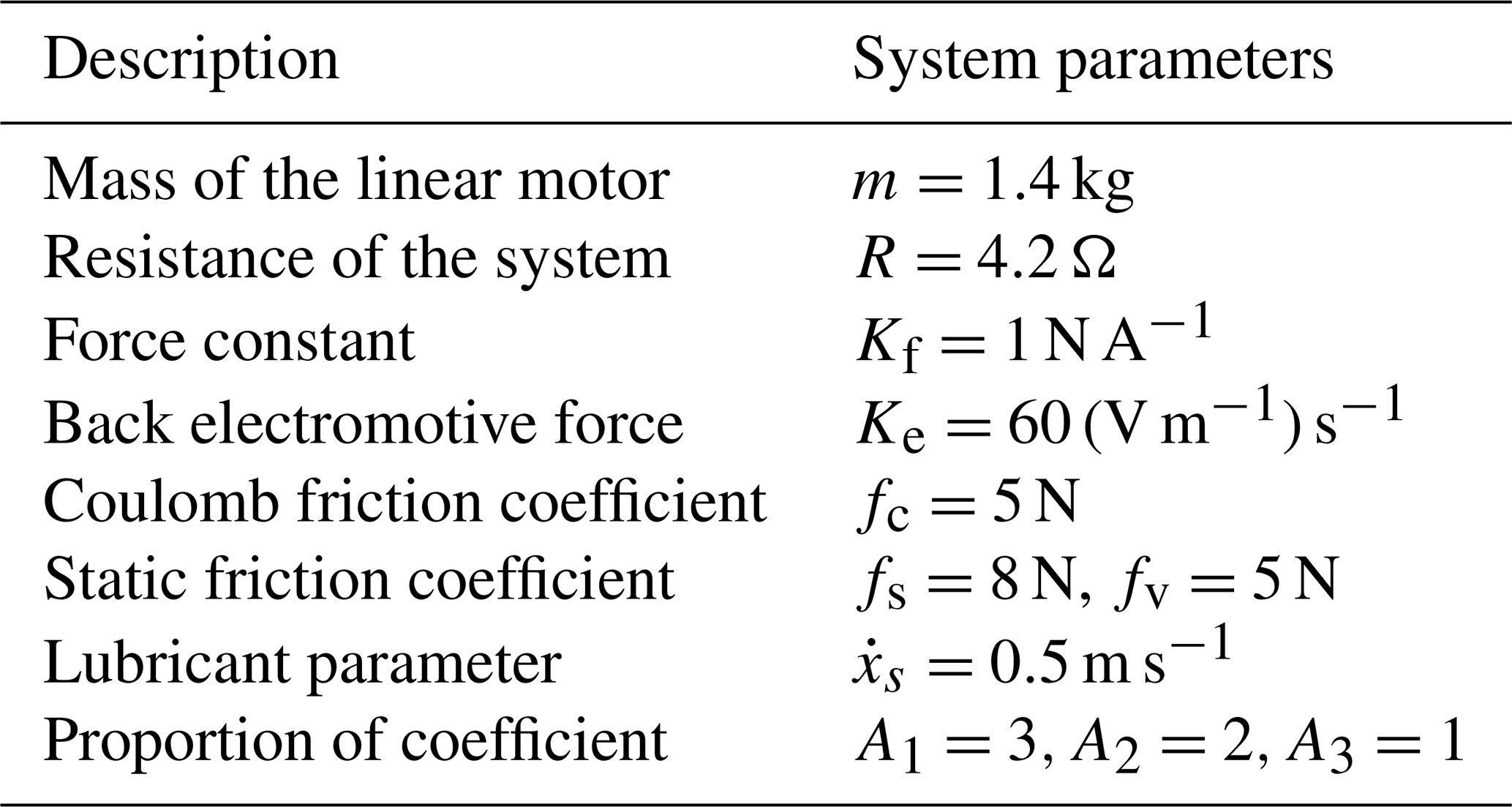
The control ratios (11) and (28) of the PMLM system satisfying the U–K equation constraints in Eq. (2) and inequality constraints in Eq. (13) are established in MATLAB/Simulink. In order to better illustrate the validity of the proposed inequality constraint, the performance of PMLM trajectory tracking of these two methods is compared. All the simulations are implemented by using ode45 on the MATLAB platform. The physical parameters of the PMLM considered in the simulations are described as follows.

Table 1 Simulation parameters and variables for the PMLM system.

In the simulations, we use the step and sinusoidal signal response to evaluate the dynamic characteristics and the ability to deal with uncertainty of the U–K controller under both inequality and inequality constraints.

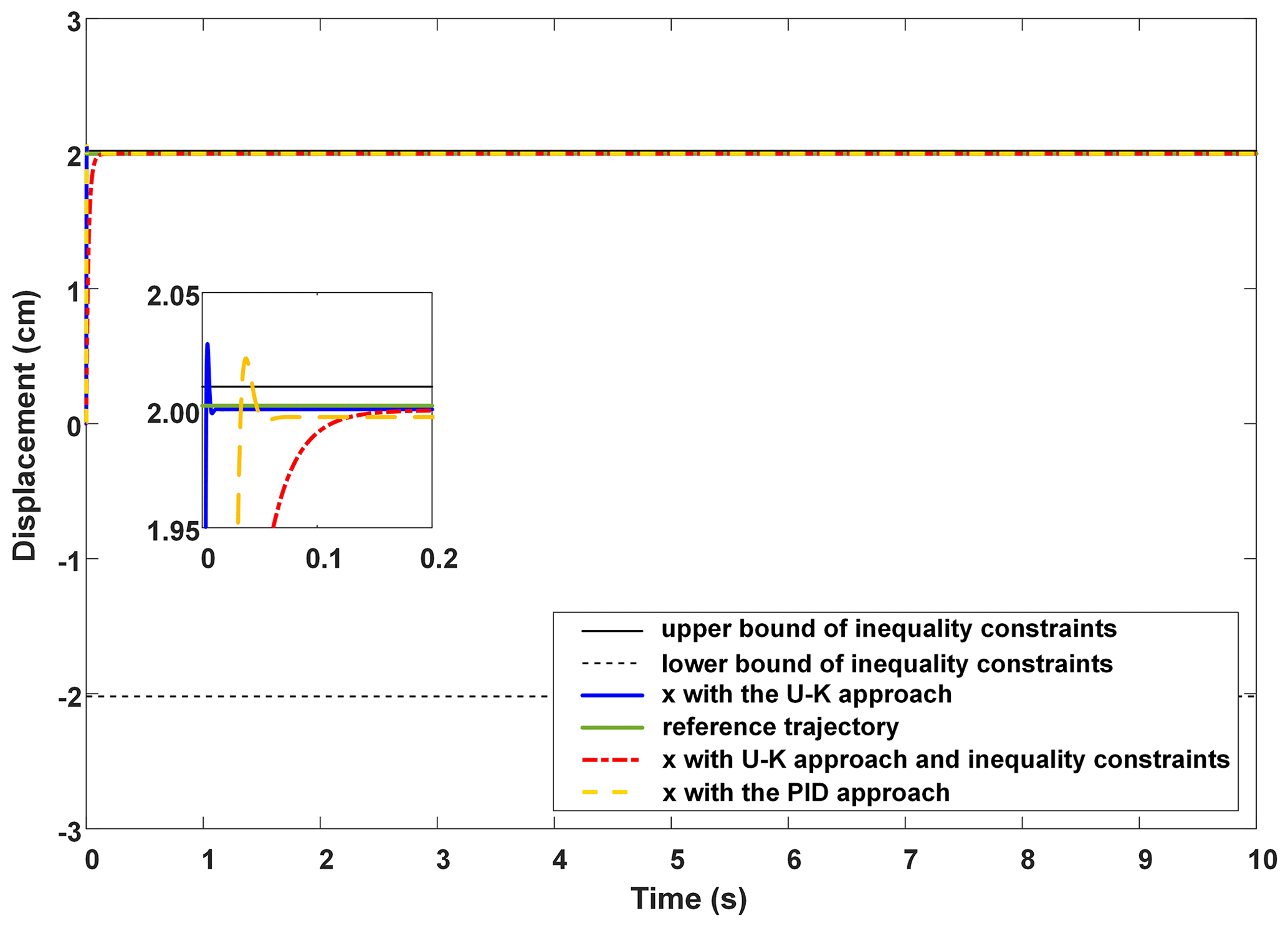
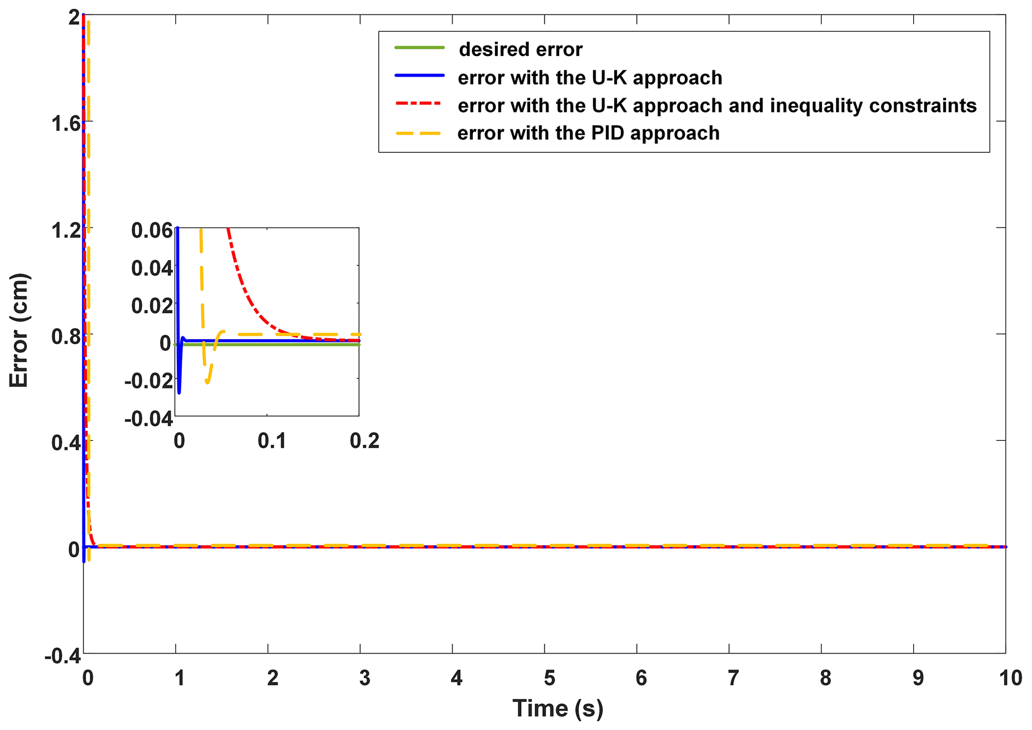
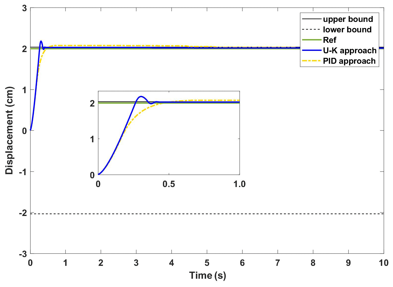
(i) Step response

The step signal utilized in this section is shown as follows:

$$\begin{array}{}\text{(67)}& x=\mathrm{2}\mathrm{cm}.\end{array}$$

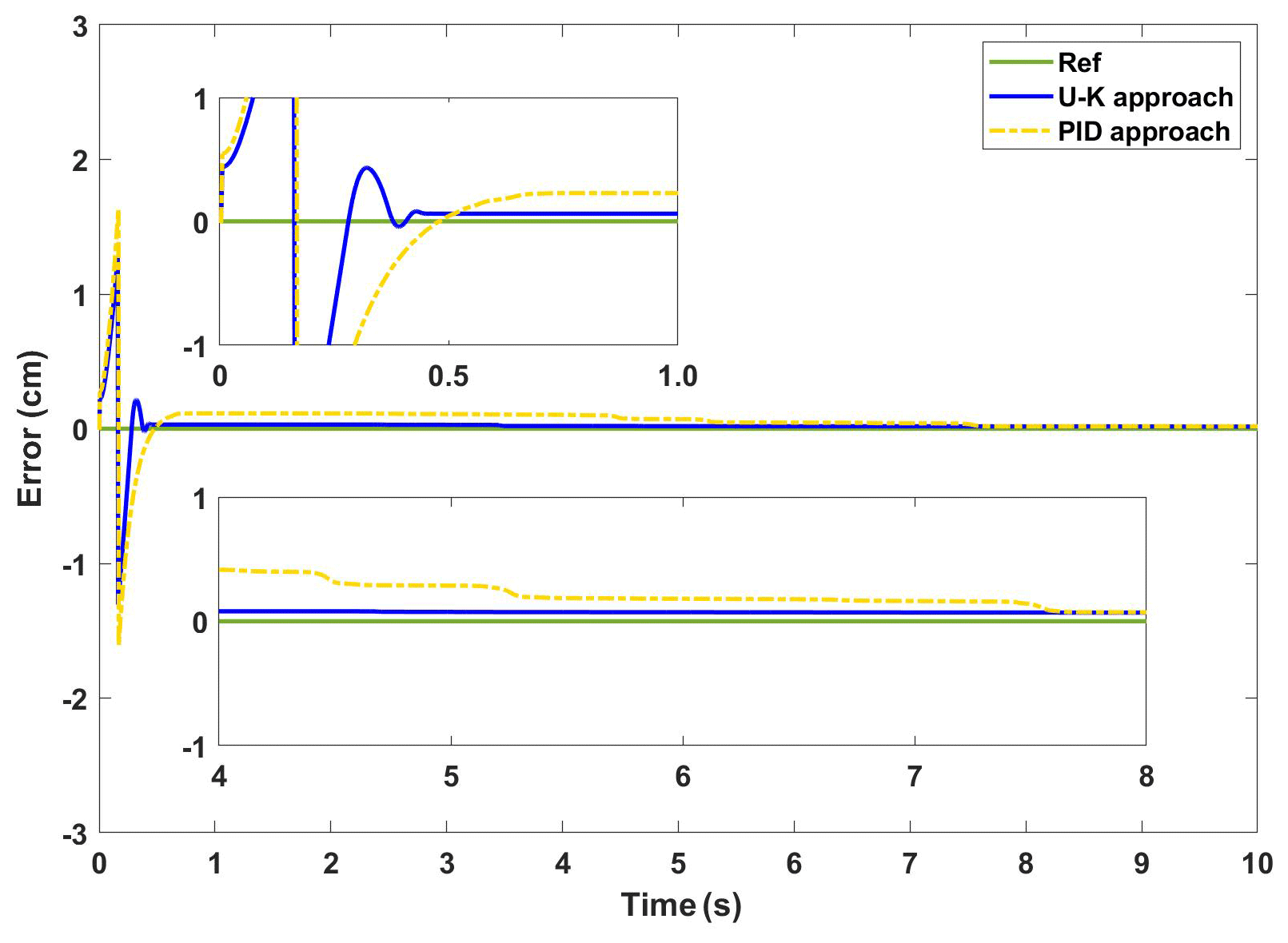
We set the position x as the limit of the motor to $[-\mathrm{2.01},\mathrm{2.01}]$. The step response of the PMLM system is shown in Fig. 2. Figure 3 shows the trajectory error. We can see that the proposed inequality constrained control method (see the red line in Figs. 2 and 3) can restrict the tracking trajectory within the boundaries on the premise of ensuring the control accuracy. However, the tracking speed of the proposed method is inferior to the U–K equality constraint (see the blue line) and PID (see the yellow line). Specifically, the U–K equality constraint and PID method both have an obvious out-of-bounds result. For example, U–K equality constraint has an out-of-bounds result of about 0.01 s, with a maximum error of 0.03 cm, while the PID method also has an out-of-bounds result of about 0.02 s, with a 0.025 cm error. Compared with those two methods, the U–K inequality constraint control method converges to the reference trajectory gradually without any out-of-bounds result. But the stable tracking time of the U–K inequality constraint is 0.2 s, which is a little longer than the equality constraint (0.01 s) and PID (0.02 s).

Figure 2 PMLM displacement under the step response.

Figure 3 PMLM error under the step response.

(ii) Tracking a sinusoid signal

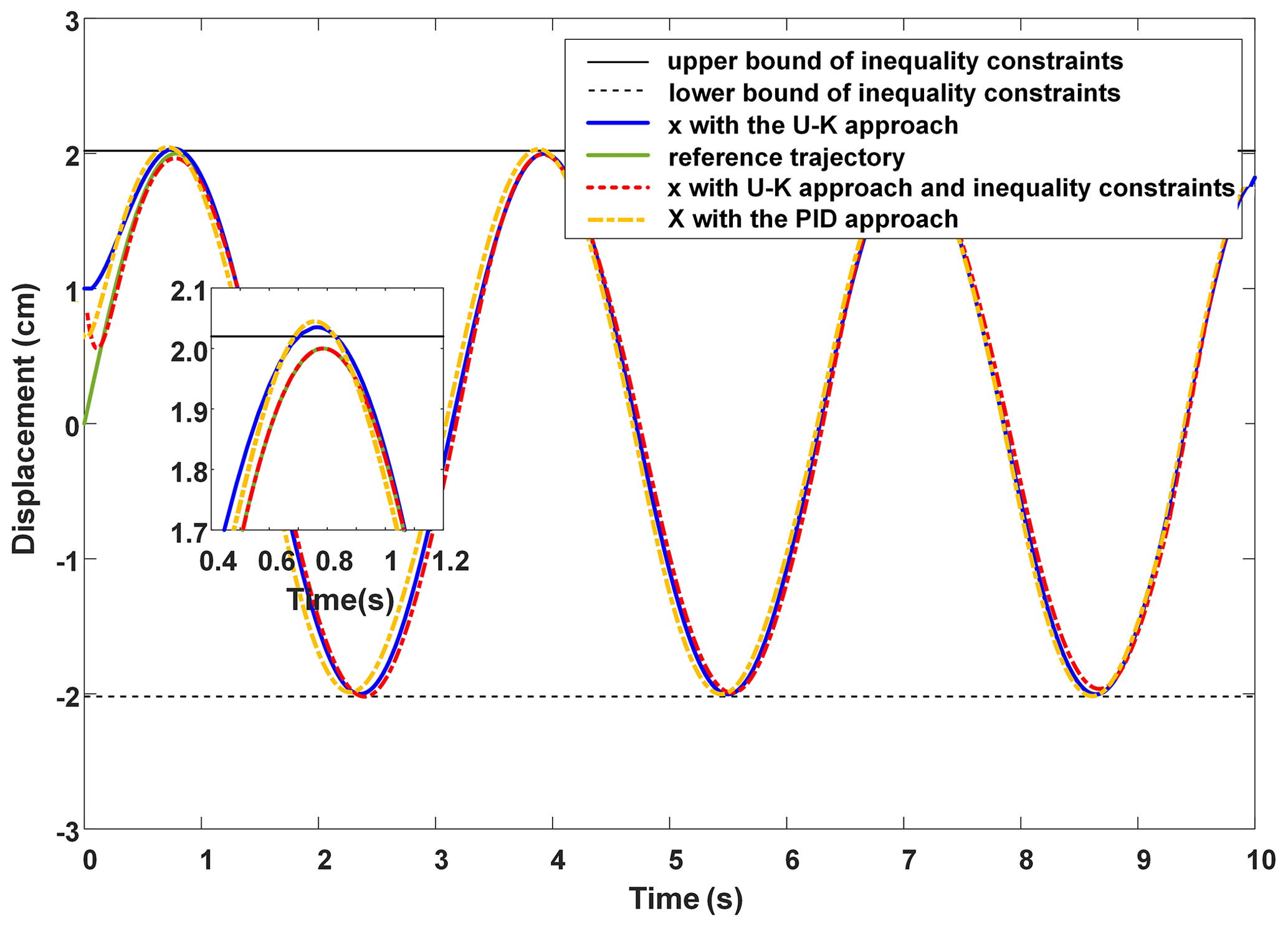
In the following simulations, we propose using the sinusoidal signal to realize sinusoidal trajectory tracking in the PMLM system. The sinusoidal signal is shown below, as follows:

$$\begin{array}{}\text{(68)}& x=\mathrm{2}\sin \left(t\right).\end{array}$$

Similarly, we restricted the position of the motor $[-\mathrm{2.01},\mathrm{2.01}]$. The curves of displacement and the displacement error of the PMLM under different control algorithms are shown in Figs. 4 and 5. It can be seen from the figures that the designed inequality constraints controller can quickly track the desired trajectory of continuous time-varying signals, and it has a good steady-state performance. The U–K and PID methods without inequality-constrained transformations have exceeded the boundaries in the period of 0.7–0.9 and 1–5 s, respectively, after which a better tracking effect can also be achieved. However, in comparison, the method with inequality constraint proposed in this paper is faster and more stable in tracking.

Figure 4 PMLM displacement under the sinusoid signal.

Figure 5 PMLM error under the sinusoid signal.

4.3.2 Experimental results

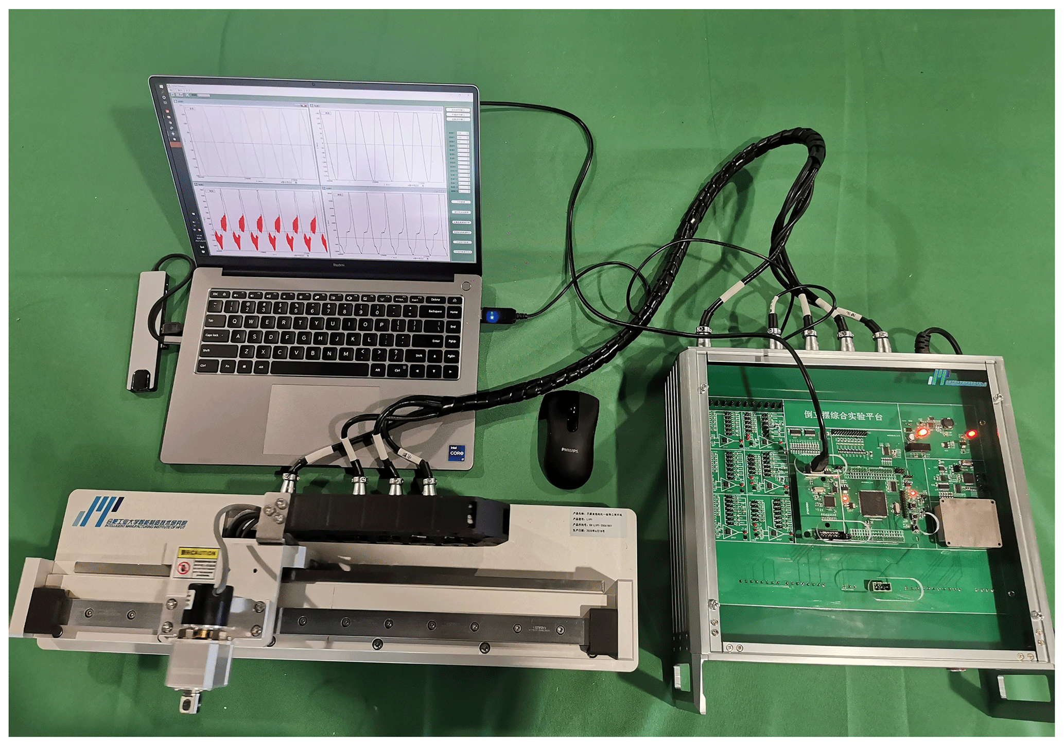
The experimental test device is shown in Fig. 6, which is mainly composed of PMLM, a cSPACE control platform, a computer with MATLAB/Simulink, a grating displacement sensor, a linear motor driver, etc. In the MATLAB environment, cSPACE can be used to observe the variables, modify the control parameters, and graphically display the control results in real time. Besides, the data collected by DSP (digital signal processing) can be saved to the disk in the form of MATLAB data files.

The parameter setting of the controller is the same as that of the simulation part, and the sampling period is 0.02 s. This real-time experiment is designed to further verify the effectiveness of the proposed control method. The following four scenarios will be considered in the experiments.

Figure 6 Experimental platform in our experiments.

(i) Transient performance of the U–K equality constraint

The step signal is added as the reference signal. Figure 7 shows the experimental results of the step response curves of U–K equality constraint and the PID method, and the corresponding error curves are shown in Fig. 8. In addition, the PMLM control input response curves are shown in Fig. 9. Comparing the experimental results, we find that the U–K equality constraint method reaches a steady state at 0.4 s, which has a certain delay compared with the simulation result in Fig. 2. Besides, in the period of 0.2–0.3 s, the U–K equality constraint method also exceeded the upper limit of the control, and then the error stabilizes within 0.01 cm without major fluctuations. In contrast, the PID method reached the stable state after 8 s, and the maximum error reached 0.4 cm during this time. Furthermore, it is clear in Fig. 9 that the initial time torque of U–K equality constraint varied greatly from 0.5 to −0.5 A. After that, the overall torque is stable, except for slight variations at some certain moments, while the PID method has a large variation.

Figure 7 Experimental results of the transient performance of U–K and PID.

Figure 8 Experimental error of the transient performance of U–K and PID.

Figure 9 The control input of the transient performance of U–K and PID.

(ii) Transient performance of the U–K inequality constraint

The experimental curves of the step response of the U–K inequality constraint and PID methods are shown in Fig. 10. Figure 11 shows the corresponding error curves of the two methods being compared. As can be seen in Fig. 10, the control method containing U–K inequality constraint can limit the motor motion displacement within the agreed boundary and can limit the overshoot well. Although the overall stability time of PID method is 0.5 s, which is shorter than that of U–K inequality constraint (0.7 s), this method is always out of bounds in the first 8 s, and the maximum tracking error even reaches 0.3 cm (please see Fig. 11). By comparison, the error of the U–K inequality constraint can be stabilized within 0.1 cm, except for the starting moment, and is stable on the whole. Figure 12 shows the control inputs of the U–K inequality constraint and PID method. The experimental results show that the fluctuation of the U–K inequality constraint is much smaller than PID after reaching the stability. Although the response time is sacrificed, the U–K inequality constraint method can restrain the motion of the motor well within the boundary and obtain better control input.

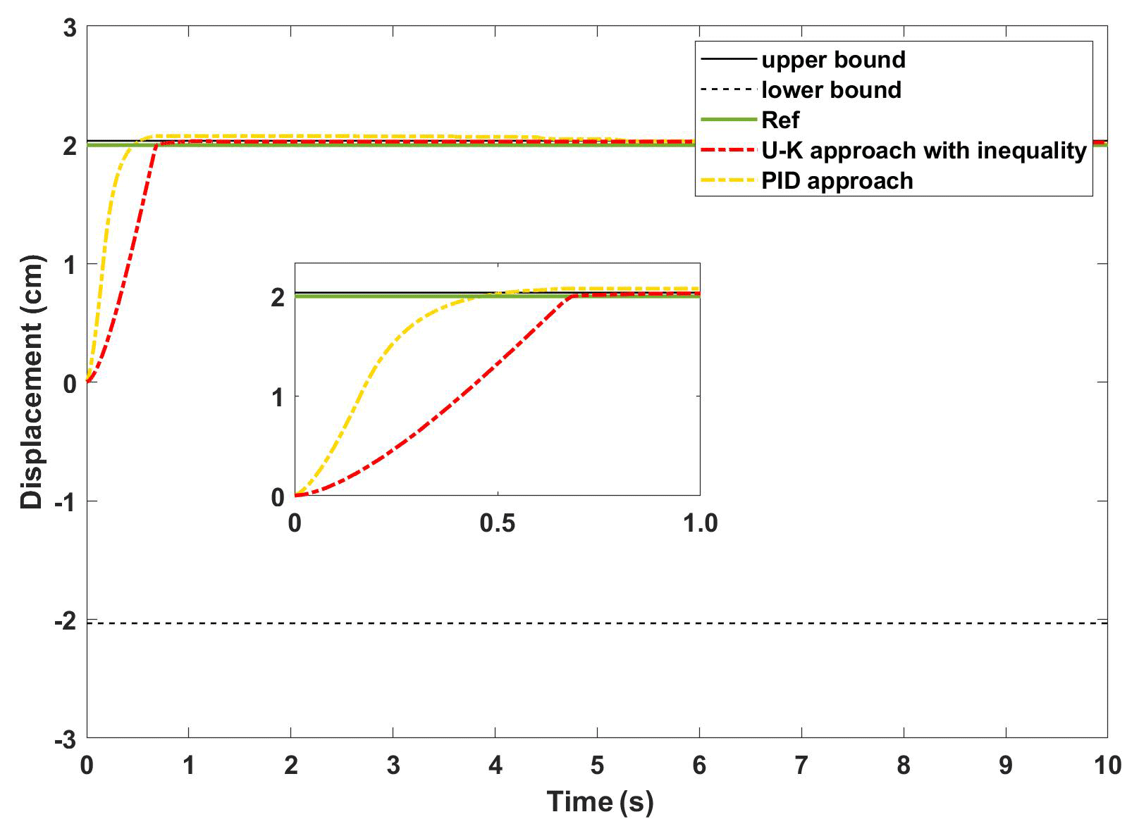
Figure 10 The experimental results of the transient performance of U–K with the inequality constraint and PID.

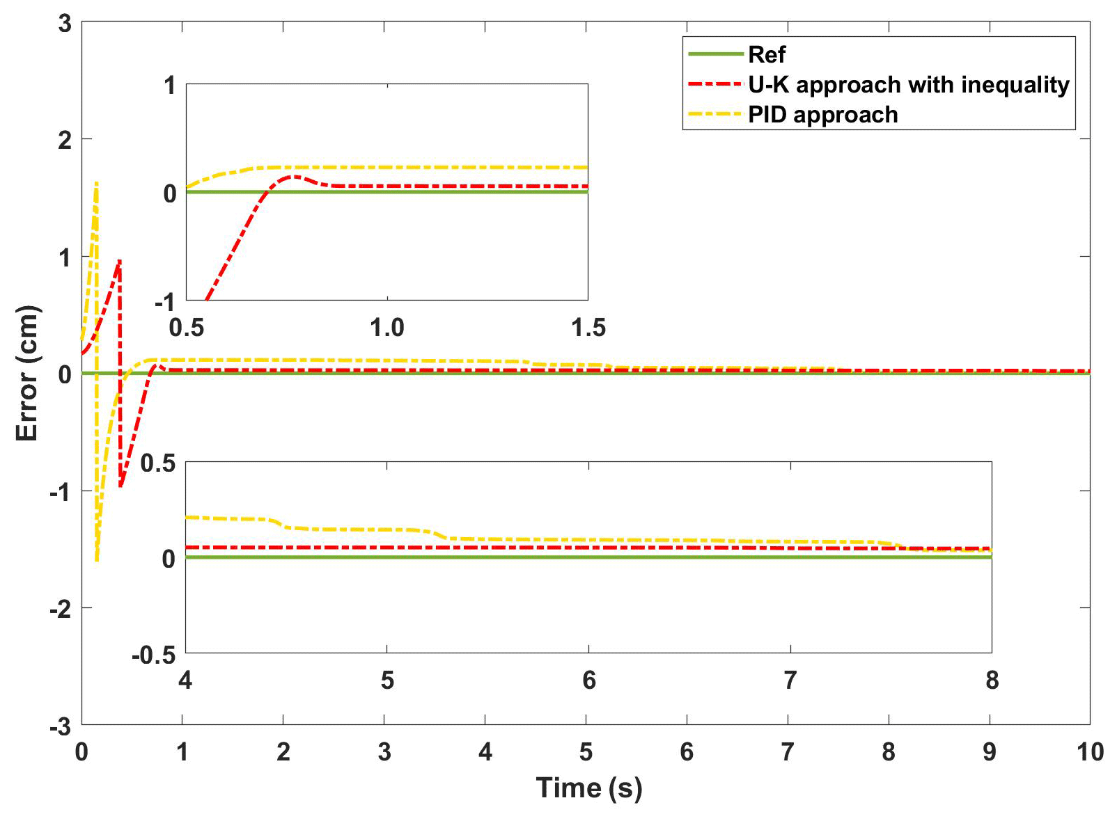
Figure 11 The experimental error of the transient performance of U–K with the inequality constraint and PID.

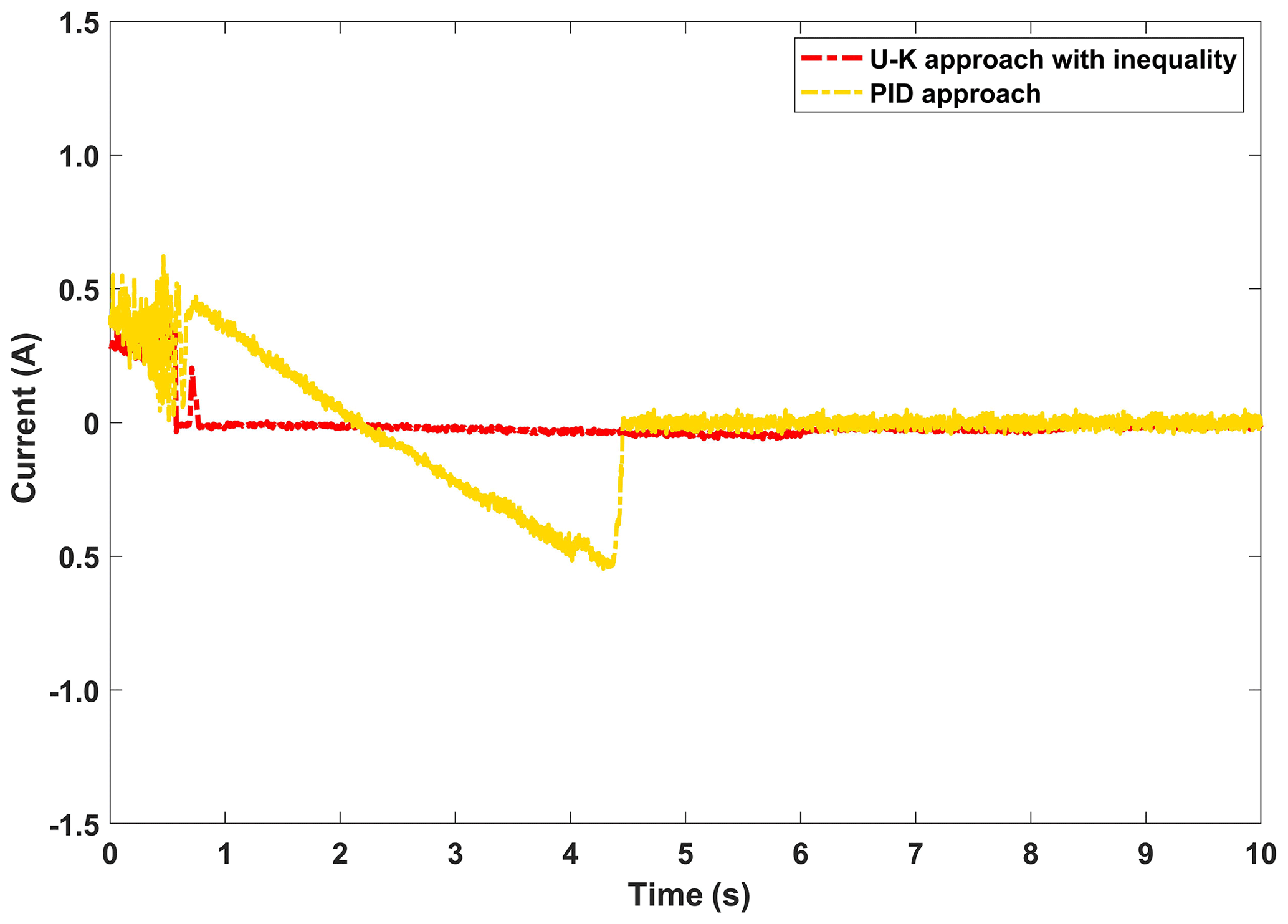
Figure 12 The control input of the transient performance of U–K with the inequality constraint and PID.

(iii) Steady-state performance of the U–K equality constraint and PID

In this part of the experiment, we mainly test the dynamic error of the linear motor. The motor was tuned to a sinusoidal trajectory at the start of the experiment, and a spike pulse interference was delivered in the first half period. Figure 13 depicts the linear motor's response time under the U–K equality constraint and the PID under a sinusoidal signal. And Fig. 14 reflects the dynamic changes in the historical errors over time for these two methods. It can be seen from Figs. 13 and 14, in the whole tracking process, that the U–K equality constraint method has higher tracking accuracy, and overshoot only occurs in the peak region of disturbance. However, the PID method has a large disturbance error when the motor starts and also obviously exceeds the control limits at the disturbance peek.

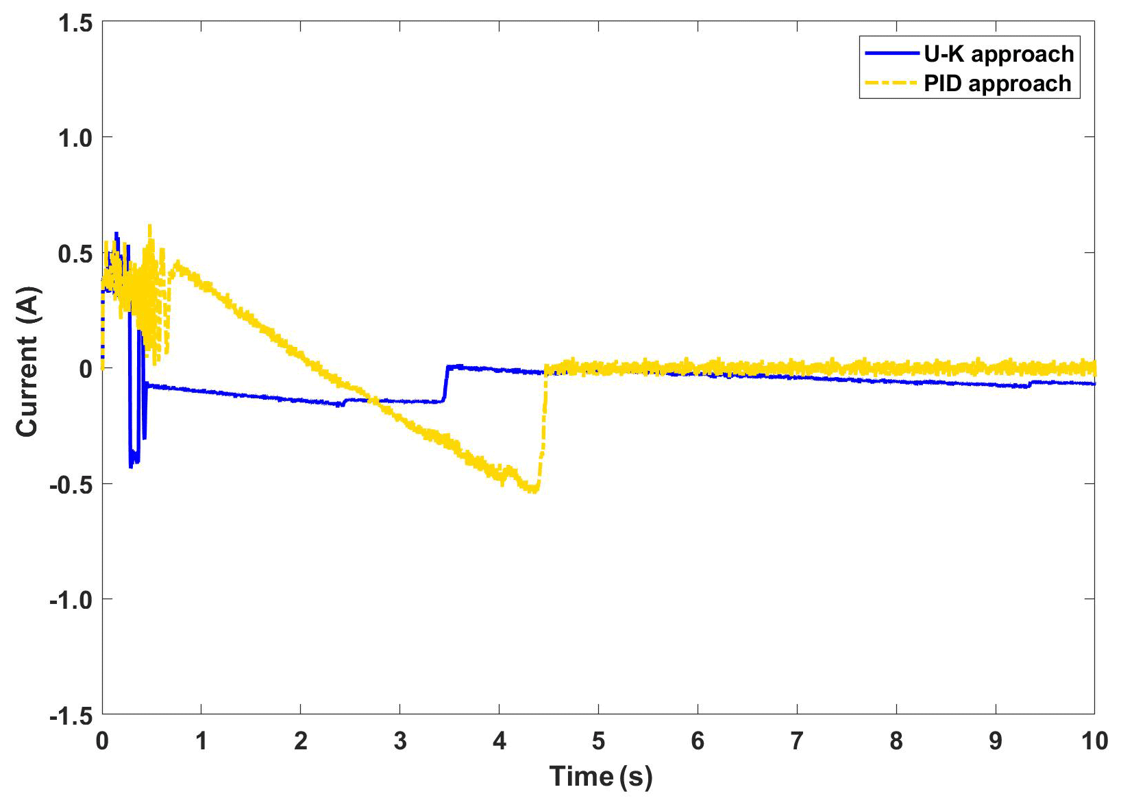
Figure 15 shows the control inputs for both methods. It is clear that the overshoot caused by the disturbance will significantly increase the control input of the PID method, with a maximum change of 1.5 A, while the influence of the disturbance on the U–K equality method is not obvious, indicating that the U–K method can better solve the problem of incompatible initial conditions. Therefore, to sum up, the constrained method containing only the U–K equation has better performance in sinusoidal wave tracking without disturbances, but this method cannot handle the overshoot caused by external disturbances.

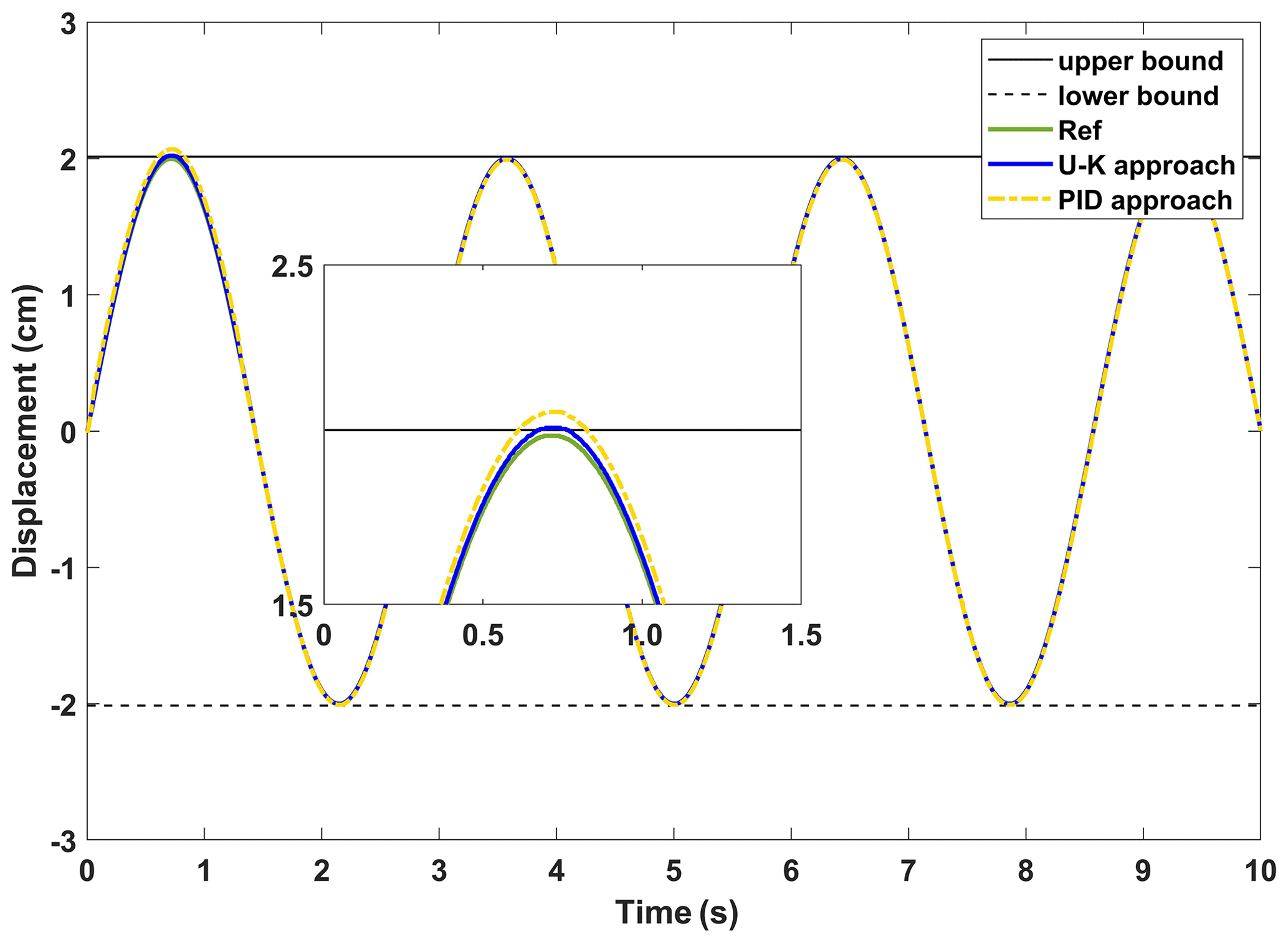
Figure 13 The experimental results of the steady-state performance of the U–K equality constraint and PID.

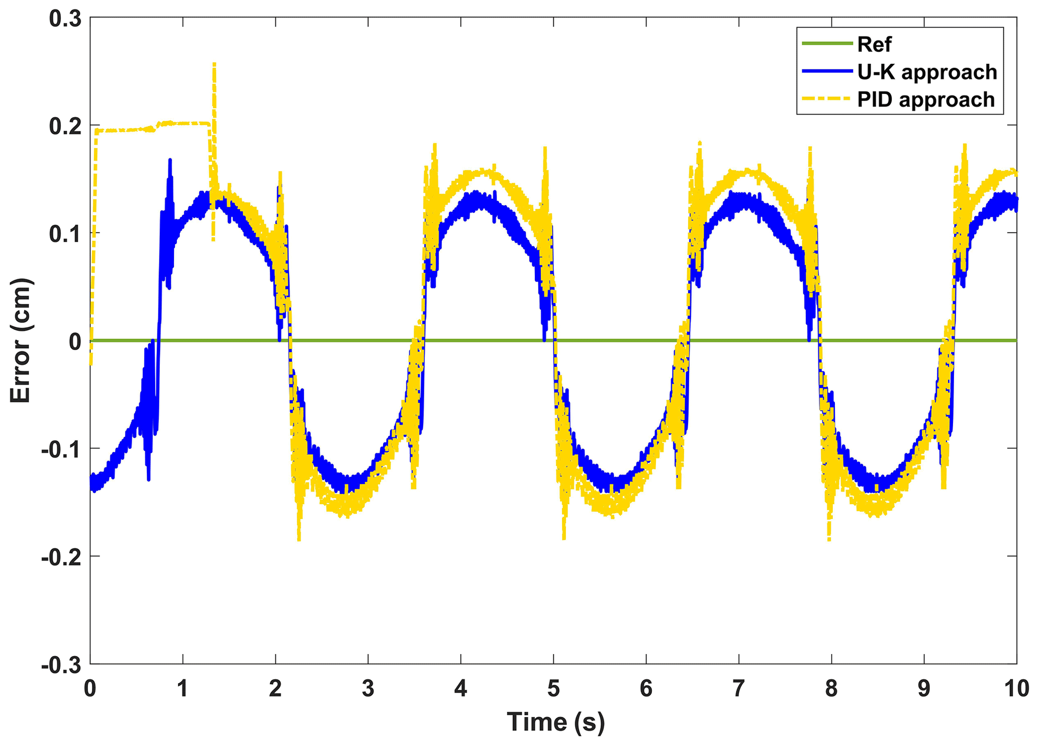
Figure 14 The experimental error of the steady-state performance of the U–K equality constraint and PID.

Figure 15 The control input of the steady-state performance of the U–K equality constraint and PID.

(iv) Steady-state performance of the U–K inequality constraint

Figures 16 and 17, respectively, show the displacement curves and error curves of the sinusoidal steady state tracking of U–K inequality constraint and PID methods. It should be noted that some anthropogenic disturbances were added in the first half of the experiment. It is obvious that the tracking trajectory of the U–K inequality constraint method basically coincides with the reference trajectory, and tracking accuracy is obviously better than that of the PID method. Moreover, even in the presence of obvious disturbances, no boundary crossing phenomenon occurs with the U–K inequality constraint. As can be seen from Fig. 17, the U–K inequality constraint method can limit the error within 0.15 cm. Because of the transformation problem of the inequality constraint, the error curve will appear at the peak value and have periodicity.

Figure 18 shows the control input of the compared methods. We can see from the figure that external interference will obviously affect the control input of the PID method. On the contrary, the U–K inequality constraint method is robust to some extent. Even if there is a certain intensity of external interference, the control input of this method basically does not fluctuate.

Finally, we can conclude from this experiment that the U–K inequality constraint can handle the overrun motion caused by external interference well, and the error is slightly reduced, which further improves the motor control's ability to handle uncertainty.

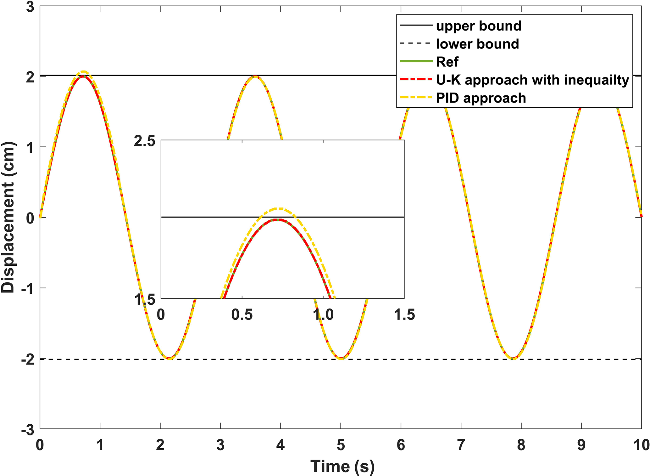
Figure 16 The experimental results of the steady-state performance of U–K with the inequality constraint and PID.

Figure 17 The experimental error of the steady-state performance of the U–K inequality constraint and PID.

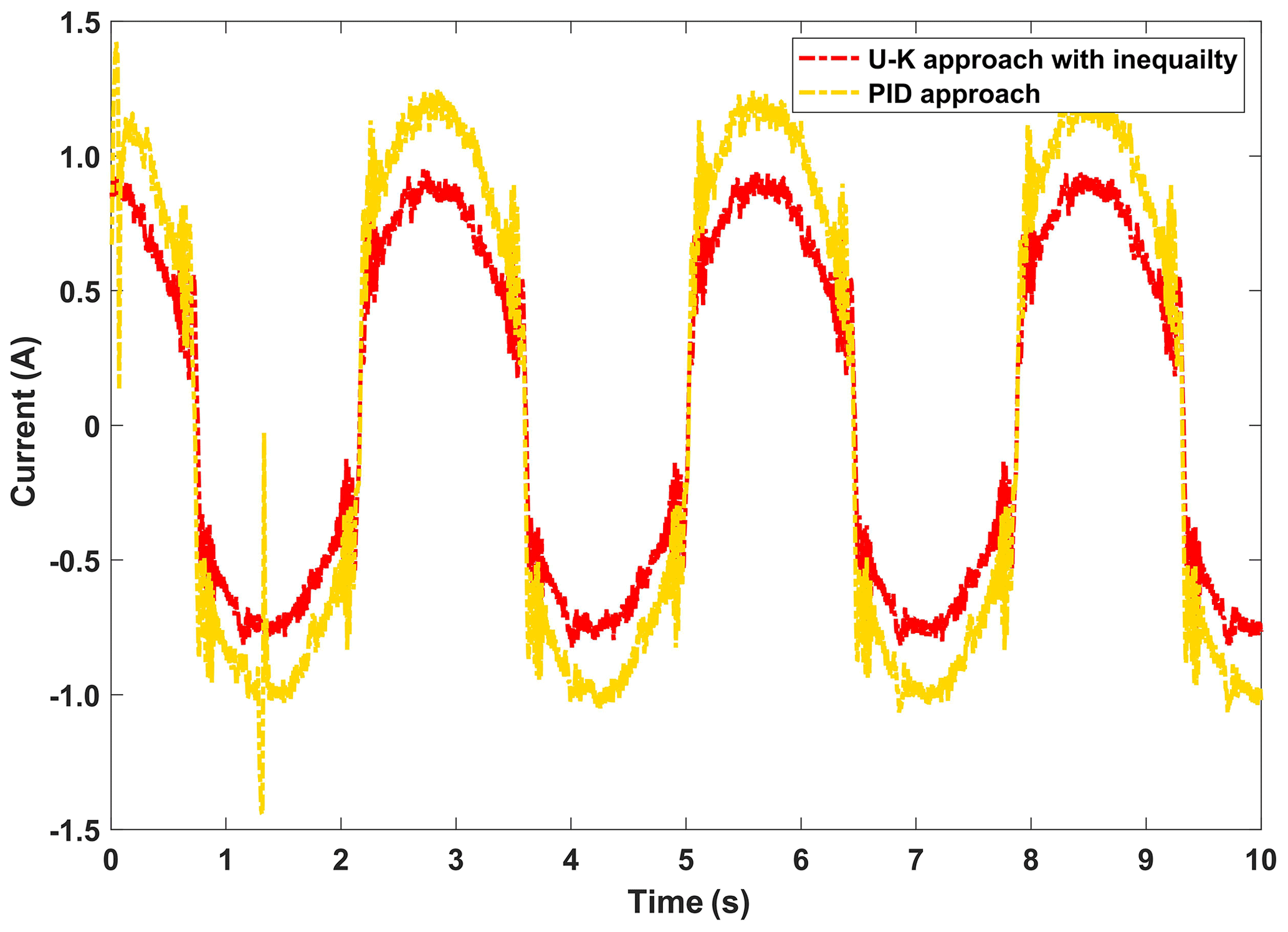
Figure 18 The control input of the steady-state performance of the U–K inequality constraint and PID.

5 Conclusions

In this paper, we propose a kind of PMLM with inequality constraints to transform a constraint tracking control method based on the equality constraint and U–K inequality status transformation. In this method, we can not only take advantage of the tangent function change to deal with the bilateral inequality constraints problem but also solve the problem of the control system of equality constraints and inequality constraints without the need for the linearization of nonlinear system. Thus, the explicit equation of the control system can be obtained without any variables, such as Lagrange multipliers.

The experimental results of PMLM experimental platform, based on cSPACE, show that, although the proposed U–K equality constraint and inequality state transition method slightly increases the tracking stabilization time, it greatly improves the control performance of the system while ensuring control safety and PMLM tracking displacement. We can see from the comparative experiments that the method has excellent performance and low control cost, which proves that the method has certain advantages and can be extended to the safety constraint control of other products. The constraint interval in this paper is open, which is determined by the conversion function we design. The tan function has the definition domain of $\mathit{\left\{}x\right|x\ne (\mathit{\pi }/\mathrm{2})+k\mathit{\pi },k\in Z\mathit{\}}$, which is only applicable to the open interval by definition. The next step is to explore the transformation of inequality-constrained closed intervals, but other transformation functions are required.