Normal contact stiffness model considering 3D surface topography and actual contact status

A normal contact stiffness model considering 3D topography and elastic–plastic contact of rough surfaces is presented in this paper. The asperities are generated from the measured surfaces using the watershed segmentation and a modified nine-point rectangle. The topography parameters, including the asperity locations, heights, and radii of the summit, are obtained. Asperity shoulder–shoulder contact is considered. The relationship of the contact parameters, such as the contact force, the deformation, and the mean separation of two surfaces, is modelled in the three different contact regimes, namely elastic, elastic–plastic and fully plastic. The asperity contact state is determined, and if the contact occurs, the stiffness of the single asperity pair is calculated and summed as the total normal stiffness of two contact surfaces. The developed model is validated using experimental tests conducted on two types of specimens and is compared with published theoretical models.

1 Introduction

Contact behaviour of mechanical joint surfaces has a great influence on a mechanical system's static–dynamic property and thermal–electrical conductivity. In order to explore the complex contact mechanisms of joint surfaces, many researchers have addressed the on-surface contact theory for a long period of time, and numerous asperity contact models have been proposed since the 1970s. The pioneering work of Greenwood and Williamson (1966) assumed that mechanical joint surfaces were represented by a population of hemispherically tipped asperities which had an identical radius of curvature. Also, they assumed that these asperities followed a Gaussian distribution, and that the contact of two mechanical joint surfaces was constituted by micro-contacts between asperities. Equations relating to the surface separation and the contact load were derived based on their assumption. After Greenwood and Williamson (1966), many other researchers continued to study asperity contact mechanisms (Sepehri and Farhang, 2008; Ciulli et al., 2008; Kim et al., 2006; Zhao and Chang, 2001; Chang et al., 1987; Whitehouse and Archard, 1970; Sun et al., 2020) and extended the asperity contact model into others, as follows: from an elastic contact situation into an elastic–plastic contact situation (Zhao et al., 2000; Chang et al., 1987; Wang et al., 2017; Ghaednia et al., 2017), from hemispherically tipped asperity into non-hemispherically tipped asperity (Ciulli et al., 2008; Jamari and Schipper, 2006), and from a Gaussian height distribution into non-Gaussian distributions (Tomota et al., 2019; Panda et al., 2015).

Most models mentioned above only concerned the relationships between normal contact load and normal interference of asperity summits. These models cannot explain some problems such as contact stiffness, contact damping, etc. (Greenwood and Wu, 2001). Meanwhile, in the real world it is rare for asperities to contact each other exactly from peak to peak. Most contact points exist on the shoulders of asperities. Sepehri and Farhang (2009, 2008) studied 2D oblique elastic shoulder–shoulder contact problems and used it in their other models, solving problems ranging from elastic–plastic interference of surfaces (Zhao et al., 2017; Shi et al., 2016), and tried to solve 3D contact problems using their 2D oblique contact model (Sepehri and Farhang, 2008; Ciavarella et al., 2006).

Based on the literature review, it can be stated that there are still some issues for the existing model in predicting the contact behaviour of the joint surfaces. On the one hand, the contact between two rough surfaces was treated as similar to that between a flat surface and a rough surface in the above models, while the shoulder–shoulder contact of asperities is more approximate to the reality in practice. On the other hand, the Gaussian distribution of asperity heights and the radii of summits are employed in the formulation of the contact; however, it cannot deal with that situation under the non-Gaussian distribution, and it cannot involve the real geometry characteristics and locations of the asperities.

This paper presents a normal contact stiffness model considering 3D topography and elastic–plastic contact of rough surfaces. The surface topography is generated from the measured data using the watershed segmentation and a modified nine-point rectangle. The topography parameters, including the asperity locations, heights, and radii of the summit, are obtained. Formula governing the shoulder–shoulder contact of asperities are derived to describe the contact behaviour in the three different contact regimes, namely elastic, elastic–plastic, and fully plastic. Based on this, an iterative computational strategy is then proposed to calculate the total normal contact stiffness at the contact surface. The developed model is validated using experimental tests conducted on two types of specimens and is compared with published theoretical models.

2 Contact model of a single asperity pair

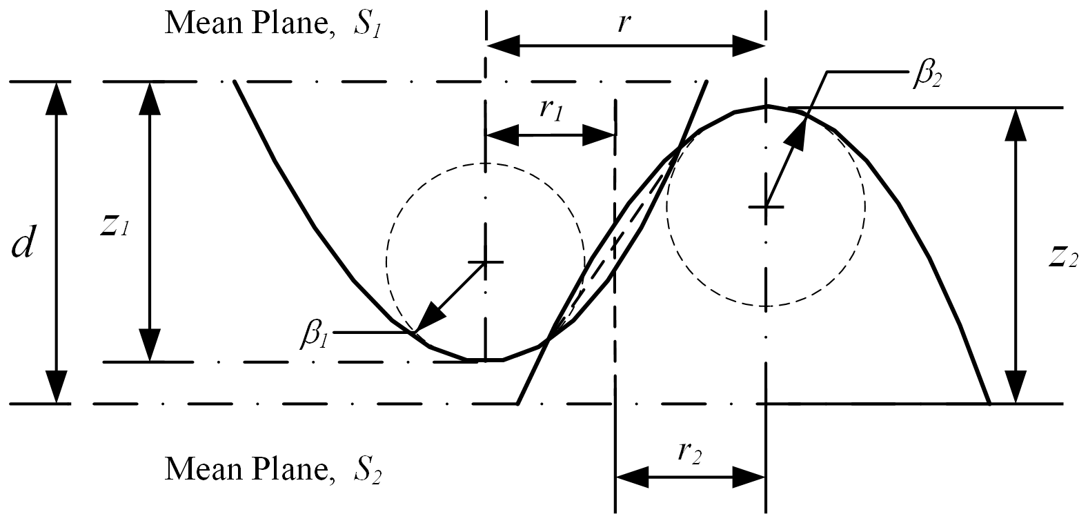
2.1 Geometrical model

The contact of two nominally flat rough surfaces mainly occurs between asperities on the mating surfaces, which are shown in Fig. 1. An asperity on surface S₁ interacts with another asperity on surface S₂; the contact point of the two asperities must be found in the midpoint of the contact region. r₁ and r₂ are the offset of the midpoint of intersecting area from the rough asperities, respectively. The curvature radius of the contact point near the rough asperity that is allowed to change according to a parabolic asperity shape can be given by the following:

$$\begin{array}{}\text{(1)}& {\mathit{\beta }}_i\left(r\right)={\mathit{\beta }}_i{\left(\mathrm{1}+{\displaystyle \frac{r^{\mathrm{2}}}{{\mathit{\beta }}_{\mathrm{s}}^{\mathrm{2}}}}\right)}^{\mathrm{3}/\mathrm{2}},i=\mathrm{1},\mathrm{2},\end{array}$$

where β_s is the sum of the curvature radius of the two contact asperities, and β_i is the equivalent curvature radius of ith contact asperity. The equivalent curvature radius of the contact asperity, with the relative distance r at the contact point, can be expressed as follows:

$$\begin{array}{}\text{(2)}& \mathit{\beta }\left(r\right)={\displaystyle \frac{{\mathit{\beta }}_{\mathrm{1}}\left(r\right){\mathit{\beta }}_{\mathrm{2}}\left(r\right)}{{\mathit{\beta }}_{\mathrm{1}}\left(r\right)+{\mathit{\beta }}_{\mathrm{2}}\left(r\right)}}=\mathit{\beta }{\left(\mathrm{1}+{\displaystyle \frac{r^{\mathrm{2}}}{{\mathit{\beta }}_{\mathrm{s}}^{\mathrm{2}}}}\right)}^{\mathrm{3}/\mathrm{2}}.\end{array}$$

Figure 1 Schematic of asperity shoulder–shoulder contact.

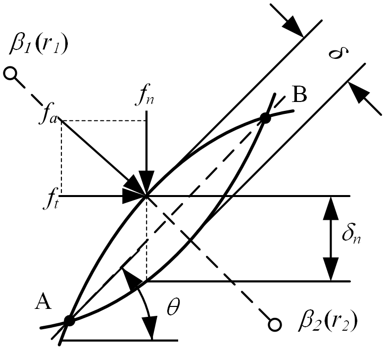
2.2 Elastic–plastic contact of asperity

For oblique contact problems, asperities interfere along an oblique line, as shown in an enlarged view of the interference in Fig. 2. f_a is the contact force, and f_n and f_t are its normal and tangential components, respectively. According to the geometrical relationship, the normal force can be given by the following:

$$\begin{array}{}\text{(3)}& f_{\mathrm{n}}=f_{\mathrm{a}}{\left(\mathrm{1}+{\displaystyle \frac{r^{\mathrm{2}}}{{\mathit{\beta }}_{\mathrm{s}}^{\mathrm{2}}}}\right)}^{\frac{-\mathrm{1}}{\mathrm{2}}}.\end{array}$$

Figure 2 Overlap region showing normal and oblique interferences.

The asperities on the rough surface experience the purely elastic, elastic–plastic, and fully plastic deformations with the gradual loading from zero to a high value, respectively. When the normal load is small, the purely elastic behaviour of the asperities is described, based on Hertz contact theory (Johnson, 1995), as follows:

$$\begin{array}{}\text{(4)}& f_{\mathrm{a}}={\displaystyle \frac{\mathrm{4}}{\mathrm{3}}}E\mathit{\beta }(r{)}^{\mathrm{0.5}}{\mathit{\delta }}^{\mathrm{1.5}}{\left(\mathrm{1}+{\displaystyle \frac{r^{\mathrm{2}}}{{\mathit{\beta }}_{\mathrm{s}}^{\mathrm{2}}}}\right)}^{\mathrm{0.75}},\mathit{\delta }\le {\mathit{\delta }}_{\text{ec}},\end{array}$$

where $\mathrm{1}/E=(\mathrm{1}-{\mathit{\upsilon }}_{\mathrm{1}}^{\mathrm{2}})/E_{\mathrm{1}}+(\mathrm{1}-{\mathit{\upsilon }}_{\mathrm{2}}^{\mathrm{2}})/E_{\mathrm{2}}$, E₁ and E₂ are the elastic modulus, and υ₁ and υ₂ are the Poisson's ratios of the contacting surfaces. δ_ec is a critical interference when initial plastic yield occurs, and it is given by Chang et al. (1987) as follows:

$$\begin{array}{}\text{(5)}& {\mathit{\delta }}_{\text{ec}}\left(r\right)=\left({\displaystyle \frac{\mathit{\pi }kH}{\mathrm{2}E}}\right)\mathit{\beta }\left(r\right),\end{array}$$

where k is the mean contact pressure factor. H is Brinell hardness of the softer material.

When the normal load is large enough, the fully plastic deformation occurs between rough asperities, and the contact load can be described based on the fully plastic contact theory (Abbott and Firestone, 1933) by the following:

$$\begin{array}{}\text{(6)}& f_{\mathrm{a}}=\mathrm{2}\mathit{\pi }\mathit{\beta }\left(r\right)H\mathit{\delta }{\left(\mathrm{1}+{\displaystyle \frac{r^{\mathrm{2}}}{{\mathit{\beta }}_{\mathrm{s}}^{\mathrm{2}}}}\right)}^{\mathrm{1.5}},\mathrm{110}{\mathit{\delta }}_{\text{ec}}<\mathit{\delta }.\end{array}$$

The normal contact load of mating asperities in the transition stage from purely elastic to full plastic deformations, namely the elastic–plastic deformation stage, can be expressed as follows (Lin and Lin, 2005; Kogut and Etsion, 2003):

$$\begin{array}{}\text{(7)}& f_{\mathrm{a}}=\left\{\begin{array}{l}\mathrm{1.03}{f}_{\text{ec}}\left(r\right){\left(\frac{\mathit{\delta }}{{\mathit{\delta }}_{\text{ec}}\left(r\right)}\right)}^{\mathrm{1.425}}{\left(\mathrm{1}+\frac{r^{\mathrm{2}}}{{\mathit{\beta }}_{\mathrm{s}}^{\mathrm{2}}}\right)}^{\mathrm{0.8625}},\\ {\mathit{\delta }}_{\text{ec}}<\mathit{\delta }\le \mathrm{6}{\mathit{\delta }}_{\text{ec}}\\ \mathrm{1.40}{f}_{\text{ec}}\left(r\right){\left(\frac{\mathit{\delta }}{{\mathit{\delta }}_{\text{ec}}\left(r\right)}\right)}^{\mathrm{1.263}}{\left(\mathrm{1}+\frac{r^{\mathrm{2}}}{{\mathit{\beta }}_{\mathrm{s}}^{\mathrm{2}}}\right)}^{\mathrm{1.1055}},\\ \mathrm{6}{\mathit{\delta }}_{\text{ec}}<\mathit{\delta }\le \mathrm{110}{\mathit{\delta }}_{\text{ec}}\end{array}\right.\end{array}$$

where f_ec is a critical force when initial plastic yield occurs, and it can be written as follows:

$$\begin{array}{}\text{(8)}& f_{\text{ec}}\left(r\right)={\displaystyle \frac{\mathrm{4}}{\mathrm{3}}}E\mathit{\beta }{\left(r\right)}^{\frac{\mathrm{1}}{\mathrm{2}}}{\mathit{\delta }}_{\text{ec}}{\left(r\right)}^{\frac{\mathrm{3}}{\mathrm{2}}}.\end{array}$$

3 Normal stiffness model of rough surfaces

3.1 Topography analysis and asperity division

The 3D surface topography could be obtained by a measurement instrument, such as a white light interferometer. The watershed segmentation method is used to analyse the surface topography (Mezghani and Zahouani, 2004). The 3D rough asperities on surface topography are considered as being a catchment basin surrounded by watershed lines. A new global algorithm for identifying the 3D rough asperity is given as follows:

1. Greyscale image. The 3D surface topography is represented as a 2D greyscale image (shown in Fig. 3a). The topography height is proportional to the greyscale value of the image; that is, the minimum height corresponds to the minimum greyscale value of zero (black), while the maximum height corresponds to the maximum greyscale value of one (white).

2. Complementary operation. Local maxima and local minima in the surface topography are interchanged, as shown in Fig. 3b. The aim is the local maxima of the surface topography height, but the local minima are found by the watershed segmentation.

3. Topography enhancement. The purpose of this step is to increase the difference between the minimum and maximum values in the greyscale images (shown in Fig. 3c).

4. Watershed segmentation. The watershed segmentation algorithm is used to divide the greyscale image into several independent regions, as shown in Fig. 3d. And then, the divided image is mapped back to 3D surface topography, as shown in Fig. 3e.

5. Rough asperity identification. A conventional nine-point peak criterion was defined as a point that is higher than its eight closest neighbouring points, as shown in Fig. 4. However, with such an asperity peak definition, the shape of the asperity peak is not necessarily regular. Points further away from the centre point can be higher than their neighbouring points and thus distort the shape of an asperity peak. In order to have a more round shape for the asperity peak, the four corner points of the asperity peak must be lower than the two neighbouring points (for each corner point). Therefore, a modified nine-point peak criterion of rough asperity is adopted in this paper. It can be mathematically defined as follows:

   $$\begin{array}{}\text{(9)}& \left\{\begin{array}{l}{z}_{i,j}>z_{i-\mathrm{1},j-\mathrm{1}},z_{i-\mathrm{1},j+\mathrm{1}},z_{i+\mathrm{1},j-\mathrm{1}},z_{i+\mathrm{1},j+\mathrm{1}}\\ z_{i-\mathrm{1},j-\mathrm{1}}<z_{i,j-\mathrm{1}},z_{i-\mathrm{1},j}\\ z_{i-\mathrm{1},j+\mathrm{1}}<z_{i,j+\mathrm{1}},z_{i-\mathrm{1},j}\\ z_{i+\mathrm{1},j-\mathrm{1}}<z_{i,j-\mathrm{1}},z_{i+\mathrm{1},j}\\ z_{i+\mathrm{1},j+\mathrm{1}}<z_{i,j+\mathrm{1}},z_{i+\mathrm{1},j}\end{array}\right.\end{array}$$

   If there is no rough asperity in the divided region, the region will be merged into the surrounding adjacent region according to the similar region-merging algorithm. It guarantees that each independent region contains a rough asperity.

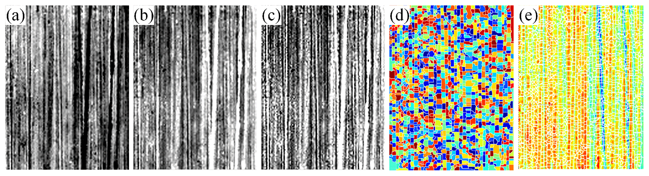
Figure 3 Rough division. (a) Greyscale image. (b) Complementary operation. (c) Topography enhancement. (d, e) Watershed segmentation.

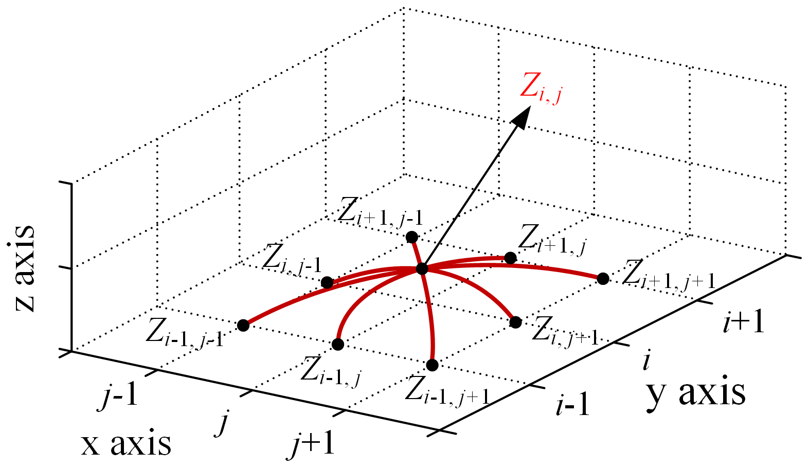
Figure 4 Modified nine-point rectangular definition of rough asperity in the independent regions.

3.2 Topography analysis and asperity division

After 3D topography analysis and rough asperity division, the summit radius of rough asperity in the kth divided region is calculated as follows:

$$\begin{array}{}\text{(10)}& {\mathit{\beta }}_k={\displaystyle \frac{\mathrm{1}}{\sqrt{{\mathit{\kappa }}_{k,x}{\mathit{\kappa }}_{k,y}-{\mathit{\kappa }}_{k,xy}^{\mathrm{2}}}}},\end{array}$$

where κ_k,x and κ_k,y are the curvatures in the x and y direction and are evaluated from the heights on the initial nine-point rectangular grid shown in Fig. 4.

$$\begin{array}{}\text{(11)}& \left\{\begin{array}{l}{\mathit{\kappa }}_{k,x}=\frac{z_{i-\mathrm{1},j}-\mathrm{2}{z}_{i,j}+z_{i+\mathrm{1},j}}{\mathrm{\Delta }{x}^{\mathrm{2}}}\\ {\mathit{\kappa }}_{k,y}=\frac{z_{i,j-\mathrm{1}}-\mathrm{2}{z}_{i,j}+z_{i,j+\mathrm{1}}}{\mathrm{\Delta }{y}^{\mathrm{2}}},\end{array}\right.\end{array}$$

and κ_k,y is the composite curvature and could be evaluated by the mixed second-order partial derivative.

$$\begin{array}{}\text{(12)}& {\mathit{\kappa }}_{k,xy}={\displaystyle \frac{\left(z_{i+\mathrm{1},j+\mathrm{1}}+z_{i-\mathrm{1},j-\mathrm{1}}\right)-\left(z_{i-\mathrm{1},j+\mathrm{1}}+z_{i+\mathrm{1},j-\mathrm{1}}\right)}{\mathrm{4}\mathrm{\Delta }x\cdot \mathrm{\Delta }y}}.\end{array}$$

Then, the coordinates of all asperities on the surface topography could be expressed mathematically with the following matrix S as follows:

$$\begin{array}{}\text{(13)}& \mathbf{S}=\left(\begin{array}{ccccccc}{x}_{\mathrm{1}}& y_{\mathrm{1}}& z_{\mathrm{1}}& {\mathit{\beta }}_{\mathrm{1}}& W_{\mathrm{11}}& W_{\mathrm{12}}& \mathrm{\cdots }\\ x_{\mathrm{2}}& y_{\mathrm{2}}& z_{\mathrm{2}}& {\mathit{\beta }}_{\mathrm{2}}& W_{\mathrm{21}}& W_{\mathrm{22}}& \mathrm{\cdots }\\ \mathrm{⋮}& \mathrm{⋮}& \mathrm{⋮}& \mathrm{⋮}& \mathrm{⋮}& \mathrm{⋮}& \mathrm{⋮}\\ x_n& y_n& z_n& {\mathit{\beta }}_n& W_{n\mathrm{1}}& W_{n\mathrm{2}}& \mathrm{\cdots }\end{array}\right),\end{array}$$

where x_i, y_i, and z_i are the coordinates of rough asperities in ith independent region of the surface topography, and β_i is the summit radius of rough asperity in the corresponding region. W_ij is the boundary point of the ith rough asperity. n is the total number of the rough asperity.

3.3 Stiffness prediction approach

The total normal load of each couple of test areas was calculated as follows:

$$\begin{array}{}\text{(14)}& F_n\left(d\right)=\sum _{i=\mathrm{1}}^N{f}_{n_i},\end{array}$$

where $f_{n_i}$ is the normal force of ith contact pair at surface separation d. N is the total number for the contact pair of the rough asperity in the nominal contact area A. Then, the total normal contact stiffness in unit area could be written as follows:

$$\begin{array}{ll}\text{(15)}& {\displaystyle }{K}_n& {\displaystyle }=-{\displaystyle \frac{\mathrm{1}}{A}}{\displaystyle \frac{\mathrm{d}\left(F_n\left(d\right)\right)}{\mathrm{d}\left(d\right)}}{\displaystyle }& {\displaystyle }=-{\displaystyle \frac{\mathrm{1}}{A}}\sum _{i=\mathrm{1}}^N\left(-{\displaystyle \frac{\mathrm{d}\left(f_{n_i}\right)}{\mathrm{d}\left(d\right)}}\right)\\ {\displaystyle }& {\displaystyle }={\displaystyle \frac{\mathrm{1}}{A}}\sum _{i=\mathrm{1}}^{\text{num}}{k}_{n_i},\end{array}$$

where the normal stiffness of a single contact pair could be calculated as follows:

$$\begin{array}{}\text{(16)}& \begin{array}{rl}{k}_{n_i}& =-{\displaystyle \frac{\mathrm{d}\left(f_{n_i}\right)}{\mathrm{d}\left(d\right)}}=-{\displaystyle \frac{\mathrm{d}\left(f_{n_i}\right)}{\mathrm{d}\left({\mathit{\delta }}_n\right)}}\times {\displaystyle \frac{\mathrm{d}\left({\mathit{\delta }}_n\right)}{\mathrm{d}\left(d\right)}}\\ & ={\displaystyle \frac{\mathrm{d}{f}_{n_i}}{\mathrm{d}{\mathit{\delta }}_n}}={\displaystyle \frac{\mathrm{d}{f}_{\mathrm{a}}}{\mathrm{d}\mathit{\delta }}}{\cos }^{\mathrm{2}}\mathit{\theta }.\end{array}\end{array}$$

The detailed procedure for predicting the normal stiffness in the unit area of the mating surfaces is illustrated in Fig. 5.

Figure 5 Flow chart for calculating the contact stiffness between two rough surfaces.

The surface topography was measured and analysed at first, and its characteristic parameters were obtained and stored with a matrix S, shown as Eq. (13). The separation distance between the two contact surfaces is specified in advance. The calculation procedure starts from the first rough asperity (i.e. the divided region on the topography) on the mating surfaces, marking i=1 and j=1, respectively. The contact status of the two rough asperities can be identified by the following formula:

$$\begin{array}{}\text{(17)}& \mathit{\delta }\left(r_{ij}\right)=\left\{\begin{array}{l}\left(z_{\mathrm{1}i}+z_{\mathrm{2}j}-d-\frac{r_{ij}^{\mathrm{2}}}{\mathrm{2}{\mathit{\beta }}_{s,ij}}\right){\left(\mathrm{1}+\frac{r_{ij}^{\mathrm{2}}}{{\mathit{\beta }}_{s,ij}^{\mathrm{2}}}\right)}^{-\frac{\mathrm{1}}{\mathrm{2}}}>\mathrm{0},\\ \text{contact}\\ \left(z_{\mathrm{1}i}+z_{\mathrm{2}j}-d-\frac{r_{ij}^{\mathrm{2}}}{\mathrm{2}{\mathit{\beta }}_{s,ij}}\right){\left(\mathrm{1}+\frac{r_{ij}^{\mathrm{2}}}{{\mathit{\beta }}_{s,ij}^{\mathrm{2}}}\right)}^{-\frac{\mathrm{1}}{\mathrm{2}}}\le \mathrm{0},\\ \text{no contact}\end{array}\right.\end{array}$$

where the misalignment r_ij of two rough asperities can be calculated as follows:

$$\begin{array}{}\text{(18)}& r_{ij}=\sqrt{{\left(x_{\mathrm{1}i}-x_{\mathrm{2}j}\right)}^{\mathrm{2}}+{\left(y_{\mathrm{1}i}-y_{\mathrm{2}j}\right)}^{\mathrm{2}}},\end{array}$$

where β_s is the sum of the radius curvature of the following two mating asperities:

$$\begin{array}{}\text{(19)}& {\mathit{\beta }}_{\mathrm{s},ij}={\mathit{\beta }}_{\mathrm{1}i}+{\mathit{\beta }}_{\mathrm{2}j}.\end{array}$$

The numbers of the rough asperity on the mating surfaces (S₁ and S₂) are denoted by M and N, respectively. Therefore, this algorithm was iterated M and N times until all rough asperities could be traversed. Then, the normal stiffness of the mating rough surface can be predicated. All of the above processes were carried out with MATLAB (version 2016b).

4 Experimental investigation

In this section, the two types of cylindrical specimens were chosen to demonstrate the experimental measurement of normal contact stiffness. They were machined by turning and milling, respectively, and were prepared with the sizes of Φ20 mm×40 mm. The specimens are made of 2A12 material (aluminium alloy) with Young's modulus E and a Poisson's ratio υ, which are 70 GPa and 0.32, respectively. The average roughness Ra of the contact surfaces is 1.6 µm.

4.1 Surface topography measurement and analysis

The contact surfaces were measured by a confocal microscope (LEXT OLS4000; Olympus, Japan), as shown in Fig. 6. The magnification of this microscope ranges from 108 to 17 280 times. It is capable of resolving features 10 nm in size in the z direction (sample height) and 120 nm in the x–y plane. The test area size of each specimen is 1280 µm×1280 µm. Typical topographies of the two types of specimens are illustrated in Figs. 7 and 8, respectively.

Figure 6 Experimental equipment for topography measurement.

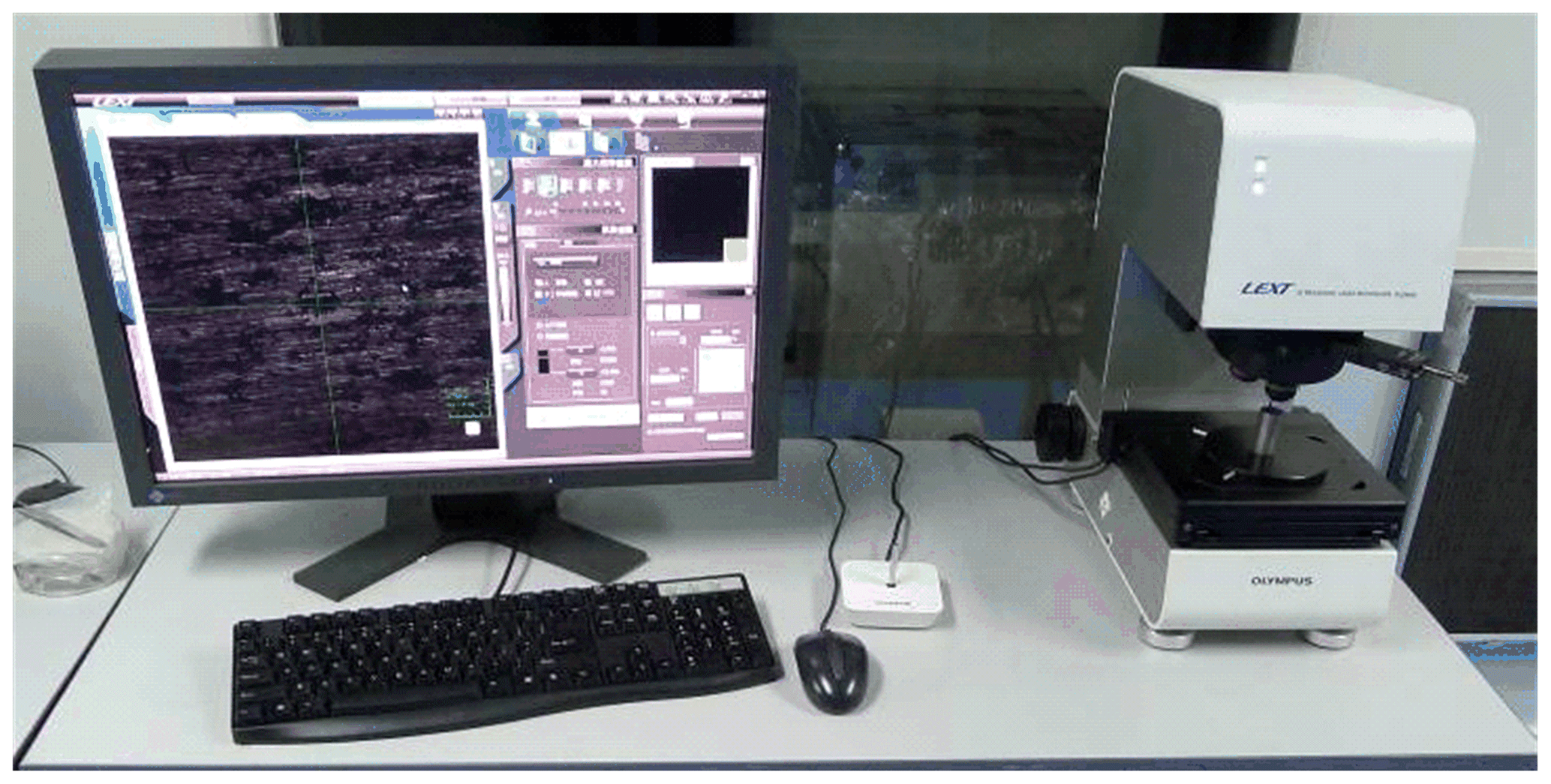
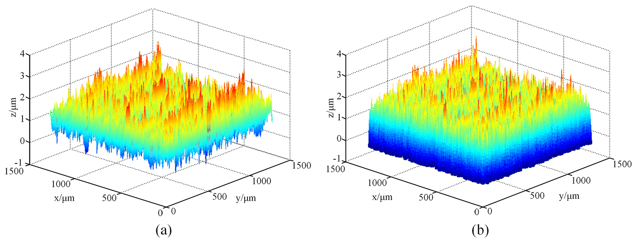
Figure 7 Typical 3D topographies of turning specimens. (a) Measured surface. (b) Watershed and fitted.

Figure 8 Typical 3D topographies of milling specimens. (a) Measured surface. (b) Watershed and fitted.

Surface topography were analysed using the method presented in Sect. 3.1. Firstly, the noise signal of the raw data was removed by wavelet analysis to obtain the real topography data of the rough surface. And then, the rough surface was divided into several subregions, based on the watershed method, each of which contains a rough peak. Finally, the rough peaks in each subregion were fitted with a rotating paraboloid, using the nine-point rectangle, and the size and spatial position of each fitted asperity were recorded.

The general statistic distributions of asperity heights and asperity radii of summits in one typical upper contact surface are illustrated in Figs. 9 and 10, respectively. It can be found that the distributions of asperity heights are fitted well with the Gaussian function, while the distributions of the asperity radii of summits are not very good. It means that the asperity radii of the summits' distribution does not strictly satisfy the Gaussian distribution.

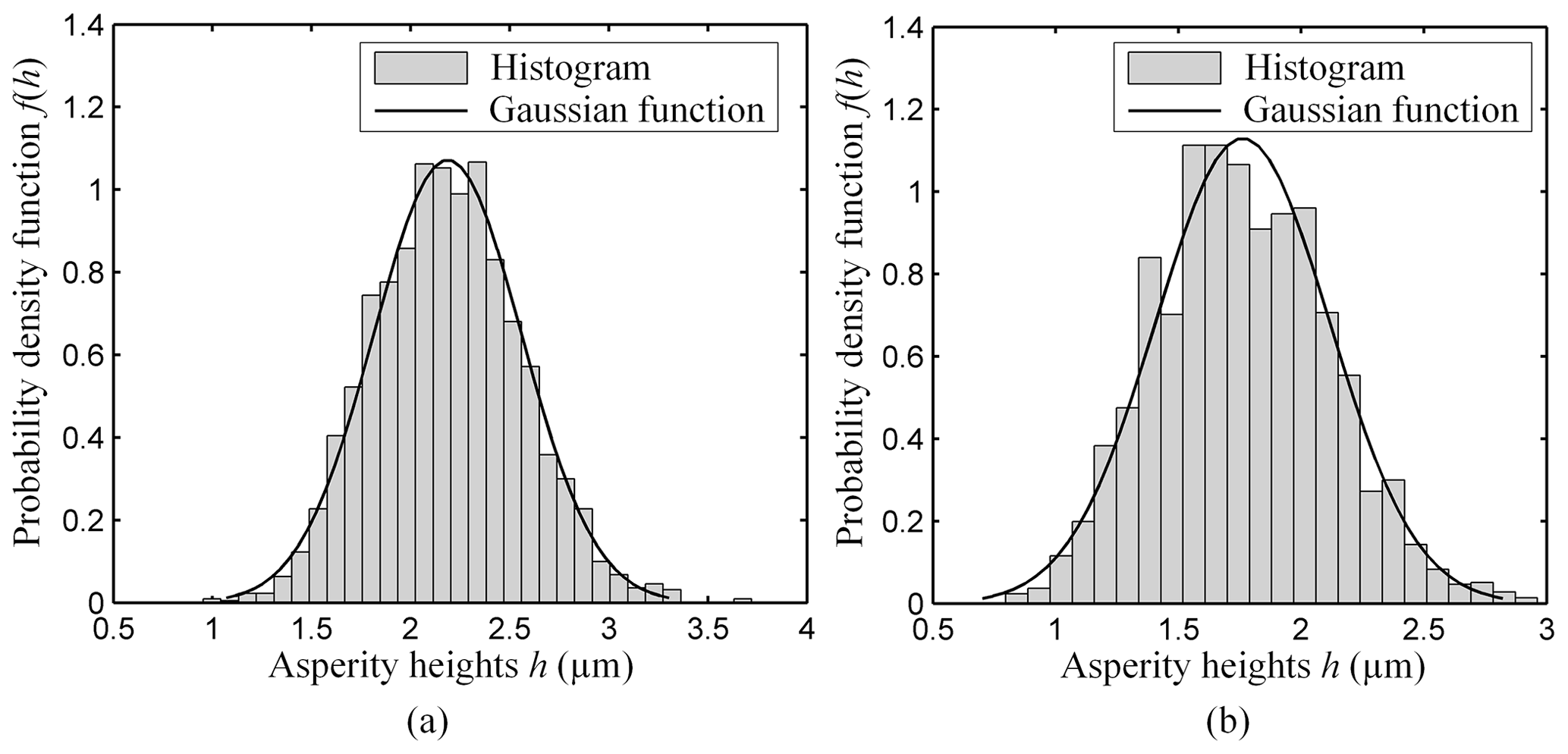
Figure 9 Statistical distribution of asperity heights of the measuring surface. (a) Turning specimen and (b) milling specimen.

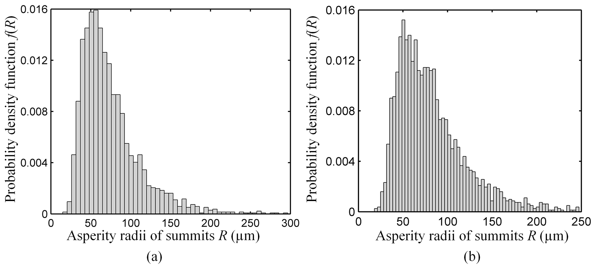
Figure 10 Statistical distribution of asperity radii of summits of the measuring surface. (a) Turning specimen and (b) milling specimen.

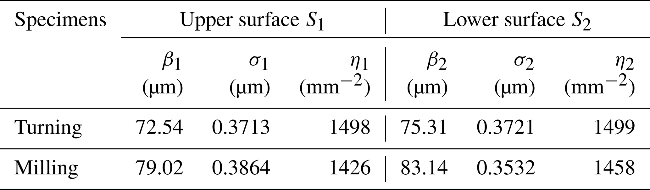
Table 1 shows the statistical parameters of the measured contact surfaces, such as asperity radii of summits β_i, standard deviation of asperity height σ_i, and asperity density η_i. $i=\mathrm{1},\mathrm{2}$ and is the upper surface and lower surface, respectively.

Table 1 Statistical parameters of the measured contact surfaces.

4.2 Normal contact stiffness measurement

The experimental validation was conducted on two short cylindrical specimens that compressed together in dry contact by the loading mechanism, as shown in Fig. 11. The experimental set-up is mainly composed of the following parts: a hydraulic jack, a force sensor, an extensometer, specimens, an adjustment mechanism, and a measurement frame. The hydraulic jack (CRSM-50; Juding Inc., China) provides the normal pressure for the contact surface of two specimens, and the value of contact loads can be obtained by the force sensor (K-450; Lorenz Messtechnik GmbH, Germany). The extensometer (3442; Epsilon Technology Corp., USA) is used to test the deformation of the two specimens during the loading process. It must be pointed that the measured value is not the contact surface deformation because it includes the solid deformation of the specimens within the original length. The adjustment mechanism consists of an adjusting screw, locking screw, self-aligning ball, etc. The specimens can be easily installed and removed by the adjusting screw and locking screw, respectively. The self-aligning ball is installed at the ball socket at the top of the upper specimen, meaning that the two surfaces are in full contact.

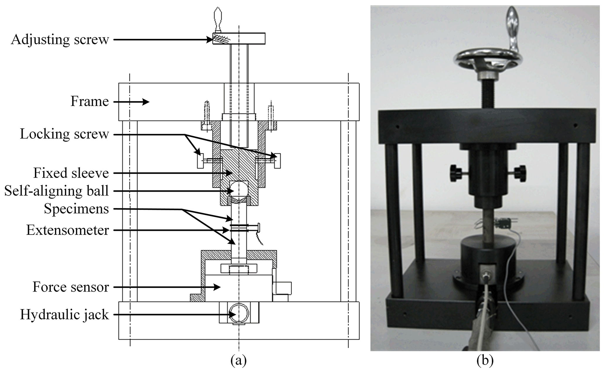
Figure 11 Experiment set-up of normal contact stiffness. (a) Schematic diagram and (b) real experiment set-up.

Based on the experimental set-up, the normal contact stiffness of the two specimens K_n can be obtained using an indirect method as follows:

$$\begin{array}{}\text{(20)}& K_n={\displaystyle \frac{\mathrm{d}F}{\mathrm{d}{\mathit{\delta }}_n}},\end{array}$$

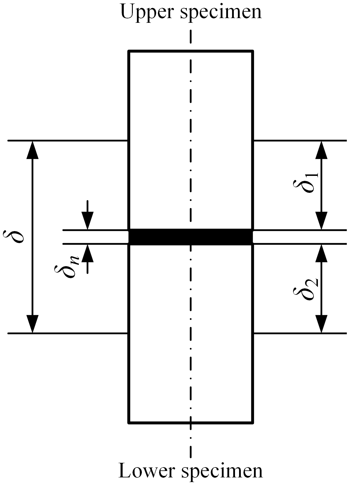
where δ_n is the normal relative deformation between the contact surfaces, as shown in Fig. 12, and can be derived indirectly by the following formula:

$$\begin{array}{}\text{(21)}& {\mathit{\delta }}_n=\mathit{\delta }-{\mathit{\delta }}_{\mathrm{1}}-{\mathit{\delta }}_{\mathrm{2}},\end{array}$$

where δ is the total deformation obtained by the extensometer. δ_i is the deformation of the contact specimen within the original length L_i, and can be calculated by the following formula:

$$\begin{array}{}\text{(22)}& {\mathit{\delta }}_i={\displaystyle \frac{F{L}_i}{E_{i}A}},i=\mathrm{1},\mathrm{2},\end{array}$$

where two specimens are differentiated by i. A is the nominal contact area. F is the normal force measured by the force sensor. E_i is the elastic modulus of the two specimens.

Figure 12 Schematic diagram of deformation between experimental specimens.

5 Results and discussion

The experimental data between the normal force and deformation and the curves fitted using a power function are shown in Fig. 13 for two types of specimens. The fitting function is given by the following:

$$\begin{array}{}\text{(23)}& {\displaystyle }& {\displaystyle }{F}_n=\mathrm{0.5636}{\mathit{\delta }}_n^{\mathrm{4.6870}}\text{for the turning specimen},\text{(24)}& {\displaystyle }& {\displaystyle }{F}_n=\mathrm{0.0006}{\mathit{\delta }}_n^{\mathrm{8.7230}}\text{for the milling specimen}.\end{array}$$

The normal contact stiffness was calculated with an indirect method of derivation with respect to deformation, and the fitting function can be expressed as follows:

$$\begin{array}{}\text{(25)}& {\displaystyle }& {\displaystyle }{K}_n=\mathrm{4.1473}{F}_n^{\mathrm{0.7866}}\text{for the turning specimen},\text{(26)}& {\displaystyle }& {\displaystyle }{K}_n=\mathrm{6.9133}{F}_n^{\mathrm{0.5005}}\text{for the milling specimen}.\end{array}$$

From the literature, there are currently three methods for calculating the normal contact stiffness of the contact surfaces, i.e. the CBE model, the KE model, and α-CBE model. In the CBE model and the KE model, the contact between two rough surfaces was simplified as being that between an ideal smooth surface and a nominally flat rough surface, while the contact between the two rough surfaces was considered for the α-CBE model. These three models calculated the normal stiffness by simple integration, based on the assumed Gaussian distribution function and the statistics parameters in Table 1.

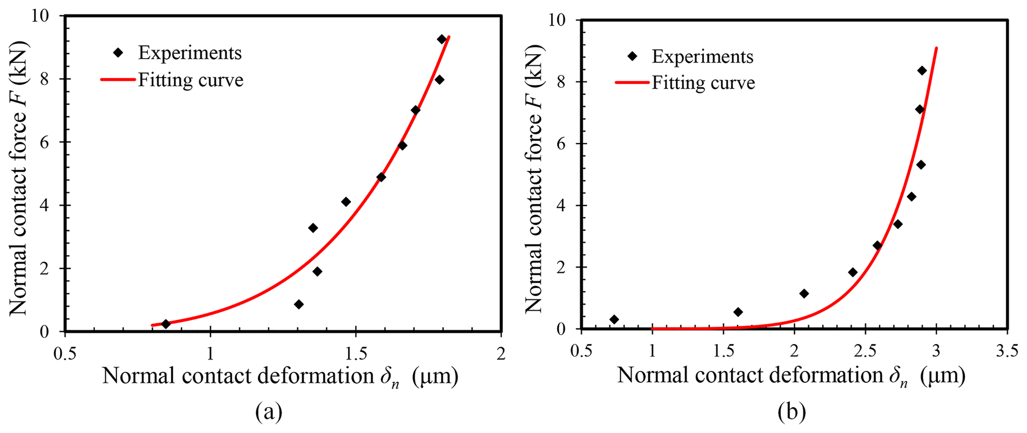
Figure 13 Experimental results and fitting curves of the relationship between normal force and deformation. (a) Turning specimens and (b) milling specimens.

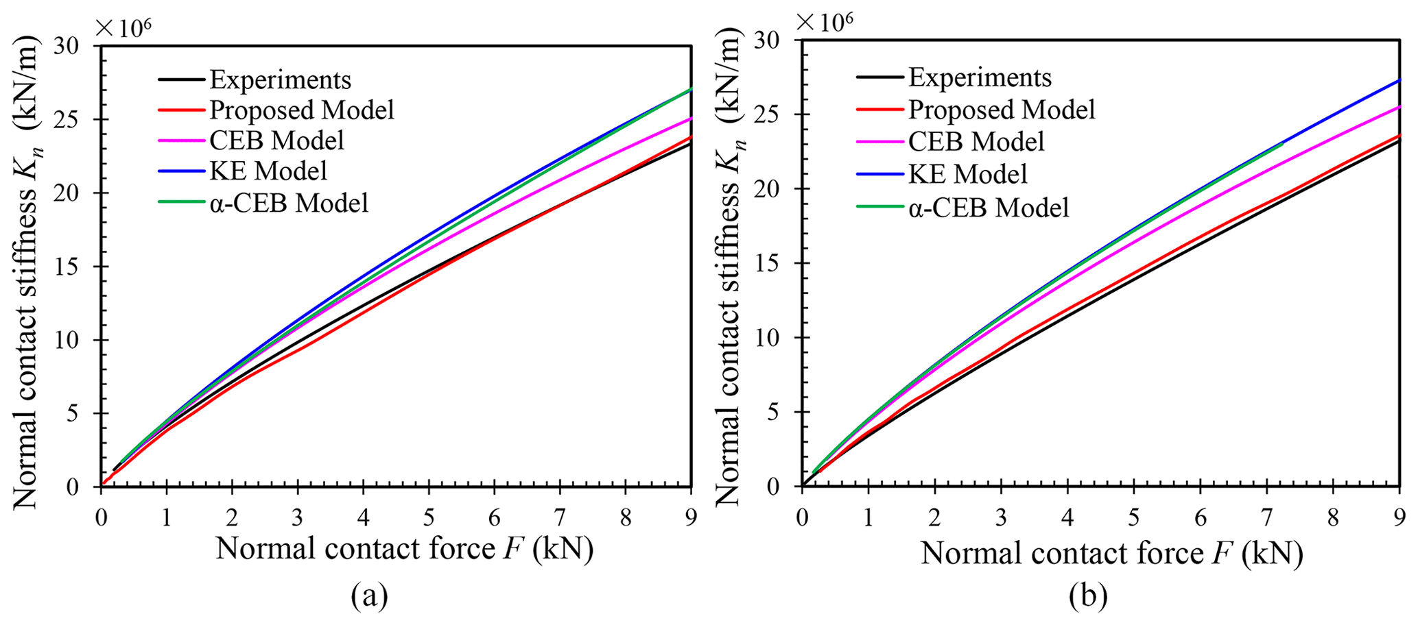
Figure 14 Comparison of normal contact stiffness predicted by a theoretical model and experimental results. (a) Turning specimens and (b) milling specimens.

The results from the proposed model in this paper were compared to those obtained from the three models and experimental tests, as shown in Fig. 14. It can be seen that the normal contact stiffness calculated by the proposed model is in good agreement with the experimental results, compared with other models. The difference in the normal contact stiffness predicted by the CBE model and KE model becomes larger as the pressure increases. This is due to more loads causing more asperities to make the plastic deformation. In the plastic state, the KE model has a higher plastic contact stiffness than the CBE model. When the normal force is small, the normal contact stiffness calculated by CBE model and α-CBE model is very close, while the difference becomes larger with the increase in the normal force. It means that the contact between two rough surfaces when calculating the normal contact stiffness cannot be treated as being that between a flat and a rough surface. The shoulder–shoulder of asperities has a greater impact on the contact stiffness.

Meanwhile, it can be observed the normal contact stiffness gradually increases with the increase in normal force. That is because the increase in the normal contact force increases the number of asperities and the actual contact area, which makes the contact surface more resistant to the deformation. Based on Eqs. (25) and (26), it can be noted that the indexes of the fitting functions are all less than one. It means that the increase rate of the normal contact stiffness with the normal force is gradually decreased. In general, very good agreement between the present model and the experimental results is found compared to the prediction of the other contact models. It can be said that the proposed model in this paper can be used to accurately predict the normal contact stiffness of the rough surfaces when considering the 3D topography surface and actual contact state. Furthermore, it can be noted that, for the joints made of 2A12 material with turning and milling, technicians can directly use Eqs. (25) and (26), respectively, to calculate the normal contact stiffness of joint surfaces. For other situations, the proposed model can be used to obtain the normal contact stiffness according to the material properties, surface roughness, normal load etc., as shown in Fig. 5.

6 Conclusions

A normal contact stiffness model of rough surfaces has been presented. In this model, shoulder–shoulder contact between asperity pairs is considered, and three different contact regimes, namely elastic, elastic–plastic, and fully plastic, are modelled. An iterative computational strategy is developed to calculate the total normal stiffness at the contact surface. The proposed model is validated using experimental tests conducted on two types of specimens, and it was compared with published theoretical models. The results show that the normal contact stiffness calculated by the proposed model is in good agreement with the experimental results when compared to the prediction of other models. Meanwhile, it could be found that the normal contact stiffness significantly increases with the increase in normal force, and the increase rate is gradually decreased. The proposed model in the paper can provide a tool for the efficient calculation of the contact force, the deformation, and the contact stiffness in engineering surfaces.