On co-estimation and validation of vehicle driving states by a UKF-based approach

It is necessary to acquire the accurate information of vehicle driving states for the implementation of automobile active safety control. To this end, this paper proposes an effective co-estimation method based on an unscented Kalman filter (UKF) algorithm to accurately predict the sideslip angle, yaw rate, and longitudinal speed of a ground vehicle. First, a 3 degrees-of-freedom (DOFs) nonlinear vehicle dynamics model is established as the nominal control plant. Then, based on CarSim software, the simulation results of the front steer angle and longitudinal and lateral acceleration are obtained under a variety of working conditions, which are regarded as the pseudo-measured values. Finally, the joint simulation of vehicle state estimation is realized in the MATLAB/Simulink environment by using the pseudo-measured values and UKF algorithm concurrently. The results show that the proposed UKF-based vehicle driving state estimation method is effective and more accurate in different working scenarios compared with the EKF-based estimation method.

1 Introduction

As we all know, a variety of vehicles has become a popular and common device in people's daily lives; meanwhile, an active safety system (ASC) of a ground vehicle plays an important role in avoiding traffic accidents as a means of guaranteeing passenger safety. However, the effective operation of ASC systems is inseparable from the accurate acquisition of vehicle driving states (Zhang et al., 2019). In general, most vehicle state information is obtained by onboard sensors. However, due to the limitation of cost and measurement methods, it is difficult for some vehicle state signals to be measured directly by sensors, which makes the estimation of vehicle states a hot topic in the field of vehicle ASCs.

Among the vehicle state signals, the sideslip angle, yaw rate, and longitudinal speed are important input variables for the vehicle ASC systems, such as the Electronic Stabilization Program (ESP), Adaptive Cruise Control (ACC), and Lane Keeping Assist (LKA), as well as the state signals that often need to be estimated (Li et al., 2020).

Currently, the common vehicle state estimation methods are usually divided into kinematics methods and dynamics methods (Selmanaj et al., 2017). Based on the relationship between the known state and the unknown state, the kinematics model-based methods calculate the unknown states by directly integrating the kinematics equation (Yamamoto et al., 1995). Generally, these methods have good accuracy for vehicle parameters, road adhesion coefficient, and driving operation. Under the condition of accurate sensor signals, these methods have high estimation accuracy for the sideslip angle in both linear and nonlinear regions (Li et al., 2014). However, the accuracy of these estimation methods is heavily dependent on the measurement accuracy of sensors, which will directly affect the estimation result of the kinematics method. What is more, due to the error accumulations in the integral process, the estimation error caused by measurement noise will increase gradually, and this will still result in the deviation of the estimated value of kinematics from its corresponding values (Piyabongkarn et al., 2009; Kim et al., 2020).

Based on the vehicle dynamics model and tire model, the dynamics methods use modern observation technology to estimate the unknown state, which can reduce the dependence on the sensor precision. The Kalman filter (KF) algorithm family are the common dynamics model-based methods, and lots of scholars have conducted extensive research on the Kalman filter family-based state estimation method. Based on an extended Kalman filter (EKF), Zong et al. (2009) established an information fusion algorithm, which gave out fusion results of vehicle state at minimum square error, and an offline simulation with real vehicle site test data in the MATLAB/Simulink environment was carried out. In Naets et al. (2017)'s research, a nonlinear least square tire parameter estimator was designed to estimate the sideslip angle and the side force of the tire based on the EKF approach, and the covariance caused by the model changes and the variation of driving conditions were also considered. Besides, Katriniok and Abel (2016) proposed an EKF-based estimator to estimate the dynamic parameters of electric vehicles, such as the longitudinal and lateral speeds, along with the yaw rate. Meanwhile, the effectiveness of this EKF-based estimator was validated through MATLAB/Simulink. Moreover, a model-based state observer (Reina et al., 2017) was developed to estimate the key motion states and the vehicle mass online; based on this, a type of vehicle parameter estimation approach was proposed by integrating with the EKF algorithm, and a comparative study between the proposed method and the KF approach was also conducted. Considering that the steering torque signal has faster and more direct response characteristics than the steering angle signal, Ma et al. (2018) proposed an EKF estimation method for the sideslip angle based on the steering torque and verified the accuracy of this method by real vehicle tests.

Like the study above, Liu et al. (2016) proposed a state estimation method for four-wheel drive vehicles based on the minimum model error (MME) criterion by combing with the EKF algorithm. It should be noticed that this method can effectively find out the dynamic tire force errors and then update the system model parameters, which improves the estimation accuracy of the vehicle state.

It is worth pointing out that the EKF algorithm is usually used to estimate the weak-nonlinear systems and simple systems. When the system is strongly nonlinear, the EKF estimation results may lead to large errors or even diverge. In addition, when the estimated system is too complex, the computational load of the EKF algorithm will increase dramatically, which may cause no solution of the Jacobian matrix (Zhou et al., 2019; Strano and Terzo, 2018). Fortunately, compared with the EKF algorithm, the unscented Kalman filter (UKF) algorithm approximates linearization by sampling instead of calculating the Jacobian matrix, which can avoid the above-mentioned problems.

In recent years, some scholars have used the UKF algorithm to estimate the driving states of vehicles. Heidfeld et al. (2019) proposed a state estimation method for all-wheel drive electric vehicles based on the UKF algorithm, which realized the comprehensive estimation of longitudinal and lateral speed, tire slip angle, and tire friction coefficient on each wheel. Based on the UKF algorithm, Song et al. (2020) designed a state observer to realize the joint estimation of vehicle states and parameters and carried out the simulation verification on the Simulink/Carsim platform. The results showed that the joint observer could effectively estimate and identify the relevant vehicle states and parameters and had a good convergence effect.

Inspired by these studies, in this paper, an effective estimation method is conducted based on the UKF algorithm in order to accurately estimate the driving states of vehicles.

This paper is organized as follows: 3 degrees-of-freedom (DOFs) vehicle dynamics modeling and problem formulation of vehicle state estimation are provided in Sect. 2, and Sect. 3 synthesizes the proposed UKF-based vehicle driving state estimation method. Besides, in Sect. 4, the validity of this UKF-based vehicle state estimation is verified by the joint simulation of CarSim and MATLAB/Simulink. Finally, Sect. 5 summarizes the conclusions and future works along this research direction.

2 3-DOFs vehicle dynamics modeling

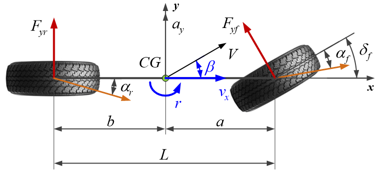
In this paper, the 3-DOFs nonlinear vehicle dynamics model is selected as the nominal model for vehicle state estimation. Based on the 2-DOFs linear vehicle dynamics model (Li et al., 2017), a dynamic model including longitudinal, lateral, and yaw motion is established, as demonstrated in Fig. 1.

Figure 1 3-DOFs vehicle dynamics model.

The 3-DOFs vehicle dynamics model can be described as follows:

$$\begin{array}{}\text{(1)}& {\displaystyle }\dot{\mathit{\beta }}={\displaystyle \frac{k_{\mathrm{1}}+k_{\mathrm{2}}}{m}}{\displaystyle \frac{\mathit{\beta }}{v_x}}+{\displaystyle \frac{a{k}_{\mathrm{1}}-b{k}_{\mathrm{2}}-m{v}_x^{\mathrm{2}}}{m}}{\displaystyle \frac{r}{v_x^{\mathrm{2}}}}-{\displaystyle \frac{k_{\mathrm{1}}}{m}}{\displaystyle \frac{\mathit{\delta }}{v_x}},\text{(2)}& {\displaystyle }\dot{r}={\displaystyle \frac{a{k}_{\mathrm{1}}-b{k}_{\mathrm{2}}}{I_z}}\mathit{\beta }+{\displaystyle \frac{a^{\mathrm{2}}{k}_{\mathrm{1}}+b^{\mathrm{2}}{k}_{\mathrm{2}}}{I_z}}{\displaystyle \frac{r}{v_x}}-{\displaystyle \frac{a{k}_{\mathrm{1}}}{I_z}}\mathit{\delta },\text{(3)}& {\displaystyle }{\dot{v}}_x=a_x+v_{y}r=a_x+\mathit{\beta }{v}_{x}r,\text{(4)}& {\displaystyle }{a}_y={\displaystyle \frac{k_{\mathrm{1}}+k_{\mathrm{2}}}{m}}\mathit{\beta }+{\displaystyle \frac{a{k}_{\mathrm{1}}-b{k}_{\mathrm{2}}}{m{v}_x}}r-{\displaystyle \frac{k_{\mathrm{1}}}{m}}\mathit{\delta },\end{array}$$

where a and b are the distances between the vehicle center of mass and the front axle and rear axle, respectively; k₁ and k₂ are equivalent cornering stiffness of the front and rear axles, respectively; m and I_z are the mass and the rotational inertia of the vehicle, respectively; v_x is the longitudinal velocity; r is the vehicle yaw rate; β is the vehicle sideslip angle; δ is the front steer angle; a_y is the lateral acceleration.

It is noted that we aim to estimate β, r, and v_x in real time by using the measured a_x and a_y as well as δ (obtained indirectly by measuring the steering wheel angle).

The system state vector x is defined as

$$\begin{array}{}\text{(5)}& \mathit{x}=[\mathit{\beta }r{v}_x{]}^T,\end{array}$$

the system input vector u is defined as

$$\begin{array}{}\text{(6)}& \mathit{u}=\left[\mathit{\delta }{a}_x\right],\end{array}$$

and the system output vector z (the measurement vector) is defined as

$$\begin{array}{}\text{(7)}& \mathit{z}=\left[a_y\right].\end{array}$$

Combining Eqs. (1)–(7), the vehicle dynamics model is expressed in the form of a state-space equation as

$$\begin{array}{}\text{(8)}& \left\{\begin{array}{l}\dot{\mathit{x}}=\mathbf{A}\mathit{x}+\mathbf{B}\mathit{u}\\ \mathit{z}=\mathbf{C}\mathit{x}+\mathbf{D}\mathit{u}\end{array},\right.\end{array}$$

where the state matrices A, B, C, and D are described in Appendix A.

3 State estimation of vehicles based on UKF

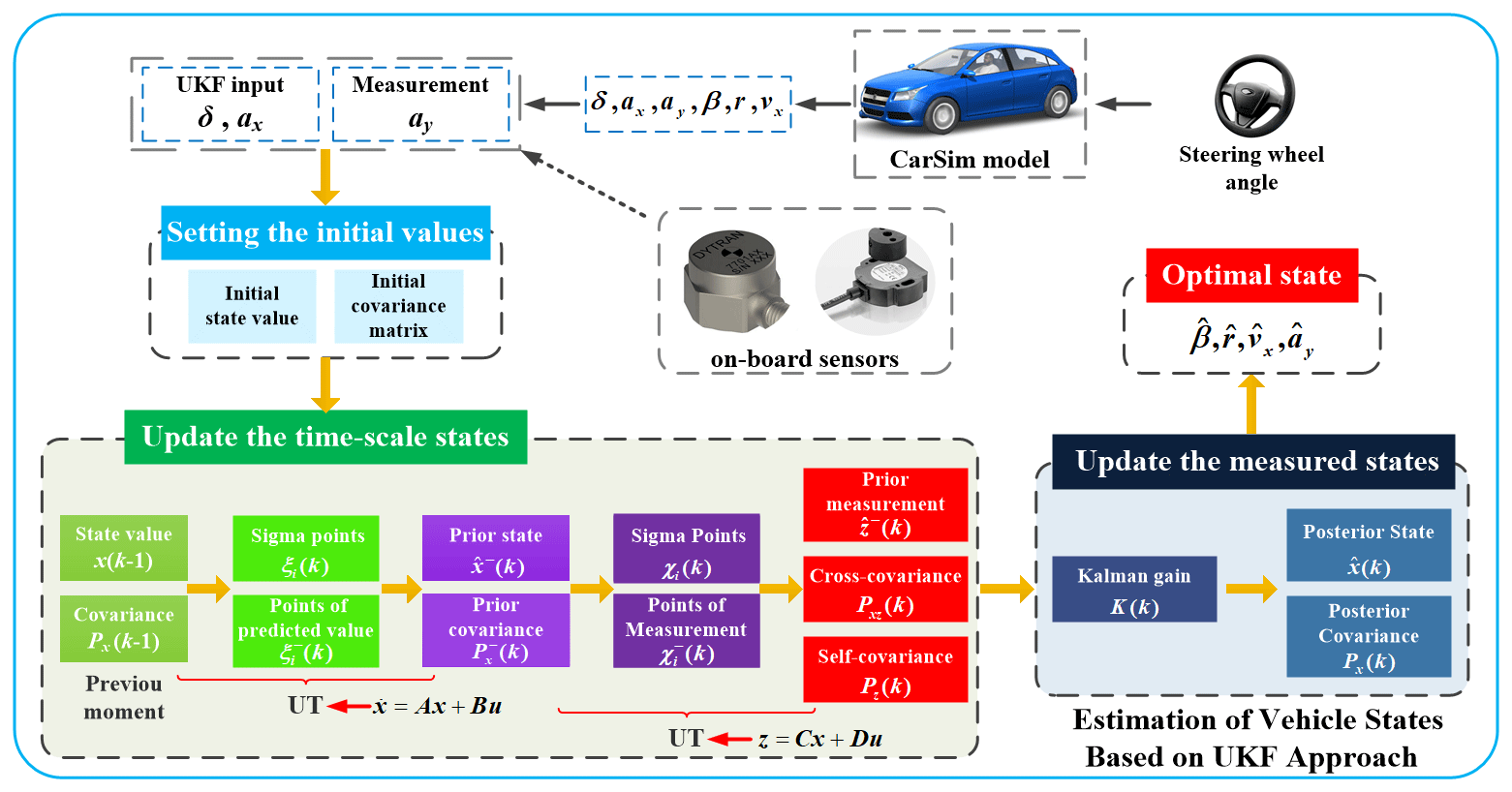
Based on the 3-DOFs vehicle dynamics model established above in Eq. (8), the UKF algorithm is applied to estimate the key driving states with the measured inputs acquired by the vehicle onboard sensors.

3.1 Unscented transformation (UT)

UT is the key of the UKF algorithm, which is a method to approximate Gaussian distribution by using a fixed number of parameter branches (Kim and Park, 2010). The UT approach can realize the linearization process of a nonlinear system by the sampling method, and it can also avoid the complicated calculation of the Jacobian matrix. The flowchart of UT is demonstrated in Fig. 2.

Figure 2 The flowchart of UT.

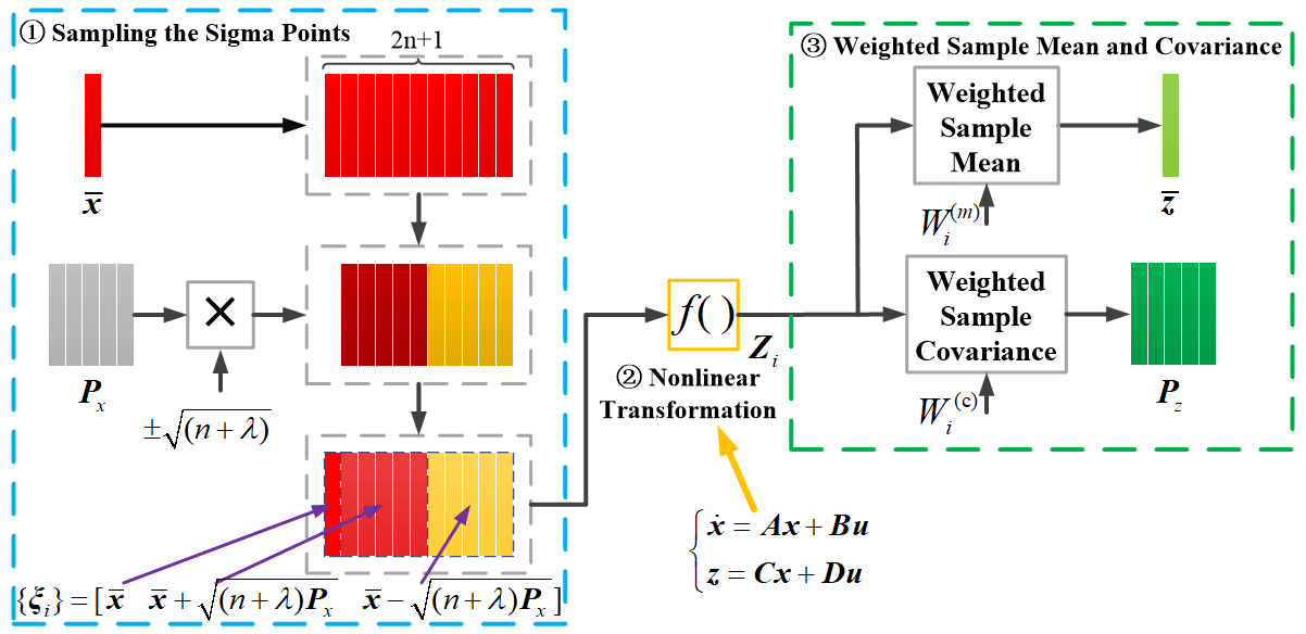
The detailed procedure of the UT is illustrated as follows.

1. Constructing the Sigma points

   According to a certain sampling strategy, a series of sampling points χ_i ($i=\mathrm{0},\mathrm{1},\mathrm{\dots },\mathrm{2}n$) are sampled from the vehicle state variables at the previous moment, which are called Sigma points. 2n is the number of sampling points, and the weights of the mean and covariance are ${\mathit{W}}_i^{\left(\mathrm{m}\right)}$ and ${\mathit{W}}_i^{\left(\mathrm{c}\right)}$, which represent the weighted coefficients of the first-order and second-order statistical properties, respectively.

2. Nonlinear transformation

   After the nonlinear transformation of χ_i, ${\mathit{\chi }}_i^{-}$ can be obtained, which can approximately represent the distribution of the prediction function $\dot{\mathit{x}}=\mathbf{A}\mathit{x}+\mathbf{B}\mathit{u}$ or measurement function $\mathit{z}=\mathbf{C}\mathit{x}+\mathbf{D}\mathit{u}$ in Eq. (8).

3. Calculating the weighted sample mean and covariance

   By calculating the weighted sum of ${\mathit{\chi }}_i^{-}$, the prior distribution of vehicle states can be approximated; that is, the mean value and covariance of the state vector x in Eq. (5) can be calculated. The crucial issue of UT is to determine the sampling strategy of Sigma points, that is, to determine the number, position, and corresponding weight of each Sigma point (Kim and Park, 2010).

Figure 3 The estimation flowchart of vehicle states based on the UKF approach.

3.2 UKF algorithm

When the one-step prediction equation of the standard KF algorithm uses UT to realize the nonlinear transformation of the mean and covariance matrix, the UKF algorithm is then constructed. The steps of the UKF algorithm are as follows.

1. Setting the initial values:

   $$\begin{array}{}\text{(9)}& \left\{\begin{array}{l}\widehat{\mathit{x}}\left(\mathrm{0}\right)=E\left[\mathit{x}\left(\mathrm{0}\right)\right]\\ \mathit{P}\left(\mathrm{0}\right)=E\left\{\left[\mathit{x}\left(\mathrm{0}\right)-\widehat{\mathit{x}}\left(\mathrm{0}\right)\right]{\left[\mathit{x}\left(\mathrm{0}\right)-\widehat{\mathit{x}}\left(\mathrm{0}\right)\right]}^{\mathrm{T}}\right\}\end{array}\right.,\end{array}$$

   wherein x(0) is the initial state value in Eq. (5).

2. Update the timescale states.

   • a.

     Sampling the Sigma points

     Based on the symmetric sampling strategy, the Sigma points and the weights of Sigma points, together with the corresponding covariance, are calculated by using the estimated state $\widehat{\mathit{x}}(k-\mathrm{1})$ and the corresponding covariance P_x(k−1) of Eq. (5) at k−1 sampling time. The Sigma points ξ_i are constructed as

     $$\begin{array}{}\text{(10)}& {\mathit{\xi }}_i\left(k\right)=\left\{\begin{array}{ll}\widehat{\mathit{x}}(k-\mathrm{1}),& i=\mathrm{0},\\ \widehat{\mathit{x}}(k-\mathrm{1})& \\ +(\sqrt{\left(n+\mathit{\lambda }\right){\mathit{P}}_x(k-\mathrm{1})}{)}_j& i=\mathrm{1},\mathrm{2},\mathrm{\dots },n,\\ \widehat{\mathit{x}}(k-\mathrm{1})& \\ -(\sqrt{\left(n+\mathit{\lambda }\right){\mathit{P}}_x(k-\mathrm{1})}{)}_j& i=n+\mathrm{1},\mathrm{\dots },\mathrm{2}n,\end{array}\right.\end{array}$$

     where n is the dimension of the state vector to be estimated; $\mathit{\lambda }={\mathit{\alpha }}^{\mathrm{2}}(n+k_{\mathrm{p}})-n$ is the proportionality coefficient, which is used to adjust the distance between $\widehat{\mathit{x}}(k-\mathrm{1})$ and Sigma points. The constant α determines the degree of dispersion of Sigma points which usually takes a small positive value. The constant k_p is the second scale parameter, which is usually set as 0 or 3−n. $(\sqrt{\left(n+\mathit{\lambda }\right)P_x(k-\mathrm{1})}{)}_j$ is the jth column of the covariance matrix square root where $j=\mathrm{1},\mathrm{2},\mathrm{\dots },n$.

     The weights of each Sigma point and the covariance matrix, i.e., ${\mathit{W}}_i^{\left(\mathrm{m}\right)}$ and ${\mathit{W}}_i^{\left(\mathrm{c}\right)}$, are determined by

     $$\begin{array}{}\text{(11)}& {\displaystyle }{\mathit{W}}_i^{\left(\mathrm{m}\right)}=\left\{\begin{array}{ll}\frac{\mathit{\lambda }}{n+\mathit{\lambda }},& i=\mathrm{0},\\ \frac{\mathrm{1}}{\mathrm{2}(n+\mathit{\lambda })},& i=\mathrm{1},\mathrm{2},\mathrm{\dots },\mathrm{2}n,\end{array}\right.\text{(12)}& {\displaystyle }{\mathit{W}}_i^{\left(\mathrm{c}\right)}=\left\{\begin{array}{ll}{\mathit{W}}_{\mathrm{0}}^{\left(\mathrm{c}\right)}+(\mathrm{1}-{\mathit{\alpha }}^{\mathrm{2}}+\mathit{\gamma }),& i=\mathrm{0},\\ \frac{\mathrm{1}}{\mathrm{2}(n+\mathit{\lambda })},& i=\mathrm{1},\mathrm{2},\mathrm{\dots },\mathrm{2}n,\end{array}\right.\end{array}$$

     where γ is the state distribution parameter, which is used to describe the distribution information of $\widehat{\mathit{x}}(k-\mathrm{1})$. In the case of Gaussian distribution, the optimal value is 2.

     When k>1, a Sigma point set containing 2n+1 sample points is constructed according to Eq. (10), which can be represented by

     $$\begin{array}{}\text{(13)}& \begin{array}{rl}{\mathit{\xi }}_i\left(k\right)& =\left\{\widehat{\mathit{x}}(k-\mathrm{1}),\widehat{\mathit{x}}(k-\mathrm{1})+(\sqrt{(n+\mathit{\lambda }){\mathit{P}}_x(k-\mathrm{1})}{)}_j,\right.\\ & \left.\widehat{\mathit{x}}(k-\mathrm{1})-(\sqrt{(n+\mathit{\lambda }){\mathit{P}}_x(k-\mathrm{1})}{)}_j\right\},\end{array}\end{array}$$

     where $i=\mathrm{1},\mathrm{2},\mathrm{\dots },\mathrm{2}n+\mathrm{1}$; $j=\mathrm{1},\mathrm{2},\mathrm{\dots },n$.

   • b.

     Calculating the sample points of the predicted values

     The prediction function $\dot{\mathit{x}}=\mathbf{A}\mathit{x}+\mathbf{B}\mathit{u}$ in Eq. (8) is used to perform the nonlinear transformation on each Sigma point to obtain the predicted value of each point, as shown in Eq. (14):

     $$\begin{array}{}\text{(14)}& \begin{array}{rl}& {\mathit{\xi }}_i^{-}\left(k\right)=f\left({\mathit{\xi }}_i\right(k),\mathit{u}(k\left)\right)={\mathbf{A}}_i{\mathit{\xi }}_i\left(k\right)+{\mathbf{B}}_i\mathit{u}\left(k\right),\\ & i=\mathrm{1},\mathrm{2},\mathrm{\dots },\mathrm{2}n+\mathrm{1}.\end{array}\end{array}$$
   • c.

     Calculating the prior state estimate and covariance

     By using the weight of Sigma points and corresponding covariance obtained from Eqs. (11) and (12), the weighted sum of the predicted sample points and covariance can be calculated; that is, the prior state and covariance can be given by

     $$\begin{array}{}\text{(15)}& {\displaystyle }{\widehat{\mathit{x}}}^{-}\left(k\right)=\sum _{i=\mathrm{0}}^{\mathrm{2}n}{\mathit{W}}_i^{\left(\mathrm{m}\right)}{\mathit{\xi }}_i^{-}\left(k\right),\text{(16)}& {\displaystyle }\begin{array}{rl}{\mathit{P}}_x^{-}\left(k\right)& =\sum _{i=\mathrm{0}}^{\mathrm{2}n}{\mathit{W}}_i^{\left(\mathrm{c}\right)}\left[{\mathit{\xi }}_i^{-}\right(k)-{\widehat{\mathit{x}}}^{-}(k\left)\right]\\ & \cdot \left[{\mathit{\xi }}_i^{-}\right(k)-{\widehat{\mathit{x}}}^{-}(k){]}^{\mathrm{T}}+{\mathbf{Q}}_k,\end{array}\end{array}$$

     wherein Q_k is the covariance matrix of system noise.

     In fact, the essence of steps (a) to (c) is to perform a UT on $\widehat{\mathit{x}}(k-\mathrm{1})$ and P_x(k−1) using the prediction function $\dot{\mathit{x}}=\mathbf{A}\mathit{x}+\mathbf{B}\mathit{u}$ in Eq. (8).

   • d.

     Calculating the prior measurement

     Return to step (a) and use the measurement function $\mathit{z}=\mathbf{C}\mathit{x}+\mathbf{D}\mathit{u}$ in Eq. (8) to carry out the second UT on ${\widehat{\mathit{x}}}^{-}\left(k\right)$ and ${\mathit{P}}_x^{-}\left(k\right)$ to obtain the prior measurement values ${\widehat{\mathit{z}}}^{-}\left(k\right)$, where the weight of each Sigma point is the same as step (a). The reconstructed Sigma point and the corresponding sampling points of prior measurement values are represented by χ_i(k) and ${\mathit{\chi }}_i^{-}\left(k\right)$, respectively. Simultaneously, the self-covariance P_z(k) of ${\widehat{\mathit{z}}}^{-}\left(k\right)$ and the cross-covariance of ${\widehat{\mathit{x}}}^{-}\left(k\right)$ and ${\widehat{\mathit{z}}}^{-}\left(k\right)$ can be calculated. The relevant calculation formulas are as follows:

     $$\begin{array}{}\text{(17)}& \begin{array}{rl}{\mathit{\chi }}_i\left(k\right)& =\left\{{\widehat{\mathit{x}}}^{-}\left(k\right),{\widehat{\mathit{x}}}^{-}\left(k\right)+(\sqrt{(n+\mathit{\lambda }){\mathit{P}}_x^{-}\left(k\right)}{)}_j,\right.\\ & \left.{\widehat{\mathit{x}}}^{-}\left(k\right)-(\sqrt{(n+\mathit{\lambda }){\mathit{P}}_x^{-}\left(k\right)}{)}_j\right\},\end{array}\end{array}$$

     where $i=\mathrm{1},\mathrm{2},\mathrm{\dots },\mathrm{2}n+\mathrm{1}$; $j=\mathrm{1},\mathrm{2},\mathrm{\dots },n$, ${\mathit{\chi }}_i^{-}\left(k\right)$ and ${\widehat{\mathit{z}}}^{-}\left(k\right)$ are as follows:

     $$\begin{array}{}\text{(18)}& {\displaystyle }{\mathit{\chi }}_i^{-}\left(k\right)=h\left({\mathit{\chi }}_i\right(k),\mathit{u}(k\left)\right)={\mathbf{C}}_i{\mathit{\chi }}_i\left(k\right)+{\mathbf{D}}_{i}u\left(k\right),\text{(19)}& {\displaystyle }{\widehat{\mathit{z}}}^{-}\left(k\right)=\sum _{i=\mathrm{0}}^{\mathrm{2}n}{\mathit{W}}_i^{\left(\mathrm{m}\right)}{\mathit{\chi }}_i^{-}\left(k\right),\text{(20)}& {\displaystyle }\begin{array}{rl}{\mathit{P}}_z\left(k\right)& =\sum _{i=\mathrm{0}}^{\mathrm{2}n}{\mathit{W}}_i^{\left(\mathrm{m}\right)}\left[{\mathit{\chi }}_i^{-}\right(k)-{\widehat{\mathit{z}}}^{-}(k\left)\right]\\ & \cdot \left[{\mathit{\chi }}_i^{-}\right(k)-{\widehat{\mathit{z}}}^{-}(k){]}^{\mathrm{T}}+{\mathbf{R}}_k,\end{array}\end{array}$$

     wherein R_k is the covariance matrix of measured noise.

     $$\begin{array}{}\text{(21)}& \begin{array}{rl}{\mathit{P}}_{xz}\left(k\right)& =\sum _{i=\mathrm{0}}^{\mathrm{2}n}{\mathit{W}}_i^{\left(\mathrm{m}\right)}\left[{\mathit{\chi }}_i\right(k)-{\widehat{\mathit{x}}}^{-}(k\left)\right]\\ & \cdot \left[{\mathit{\chi }}_i^{-}\right(k)-{\widehat{\mathit{z}}}^{-}(k){]}^{\mathrm{T}}\end{array}\end{array}$$

3. Update the posterior estimation with measured values.

   By comparing the actual measured value and the estimated measured value in Eq. (19), the Kalman gain is used to update the prior state and covariance, and we can obtain the updated value of the posterior state $\widehat{\mathit{x}}\left(k\right)$ and covariance ${\widehat{\mathit{P}}}_x\left(k\right)$ by using Eq. (22).

   $$\begin{array}{}\text{(22)}& \left\{\begin{array}{l}\mathit{K}\left(k\right)={\mathit{P}}_{xz}\left(k\right){\mathit{P}}_z^{-\mathrm{1}}\left(k\right)\\ \widehat{\mathit{x}}\left(k\right)={\widehat{\mathit{x}}}^{-}\left(k\right)+\mathit{K}\left[\mathit{z}\right(k)-{\widehat{\mathit{z}}}^{-}(k\left)\right]\\ {\widehat{\mathit{P}}}_x\left(k\right)={\mathit{P}}_x^{-}\left(k\right)-\mathit{K}\left(k\right){\mathit{P}}_z\left(k\right)\mathit{K}(k{)}^{\mathrm{T}}\end{array}\right.\end{array}$$

   By synthesizing the above derivations, the estimation flowchart of vehicle states based on the UKF approach is provided in Fig. 3.

4 Co-estimation and validation based on CarSim and MATLAB/Simulink

In order to validate the accuracy and feasibility of the proposed UKF-based vehicle states estimation approach, a co-simulation and verification in CarSim and MATLAB/Simulink is performed. First, the response curves of δ, β, r, and v_x as well as a_x and a_y are obtained in the CarSim environment under sine and fishhook maneuvers. Then, based on MATLAB/Simulink, the UKF and EKF algorithms are used to estimate β, r, and v_x, wherein δ and a_x are regarded as the input values and a_y is regarded as the measurement. Finally, the estimation results of UKF and EKF are compared with those of CarSim to judge the accuracy of the estimation of vehicle driving states by the UKF algorithm.

Table 1 The related vehicle parameters.

Figure 4 The structure of the simulator based on the UKF algorithm.

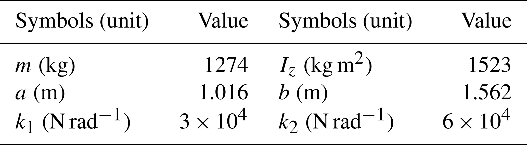
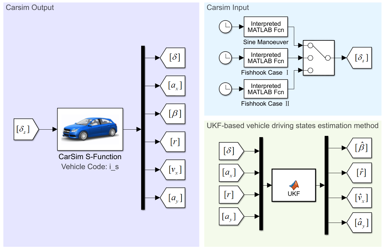
In this work, the initial value of the state covariance matrix of the UKF algorithm is set as ${\mathit{P}}_{\mathrm{0}}=I_{\mathrm{4}\times \mathrm{4}}$, and the system process noise Q_k and the measured noise R_k are given as ${\mathit{Q}}_k=\mathrm{0.001}\times I_{\mathrm{4}\times \mathrm{4}}$ and R_k=0.005, respectively. The related vehicle parameters used in the simulation model are shown in Table 1 (Li et al., 2017), and the structure of the simulator based on the UKF algorithm is shown in Fig. 4.

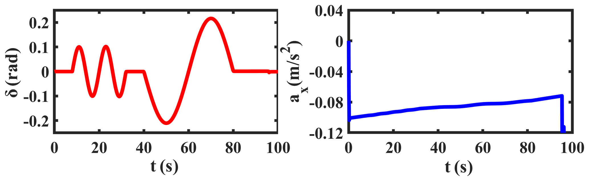
4.1 Sine manoeuver test

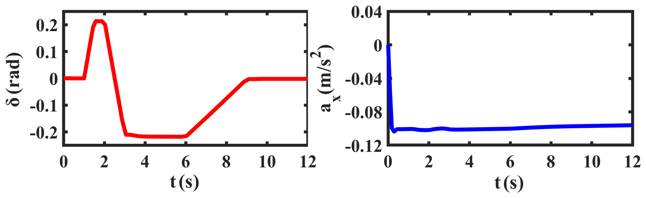
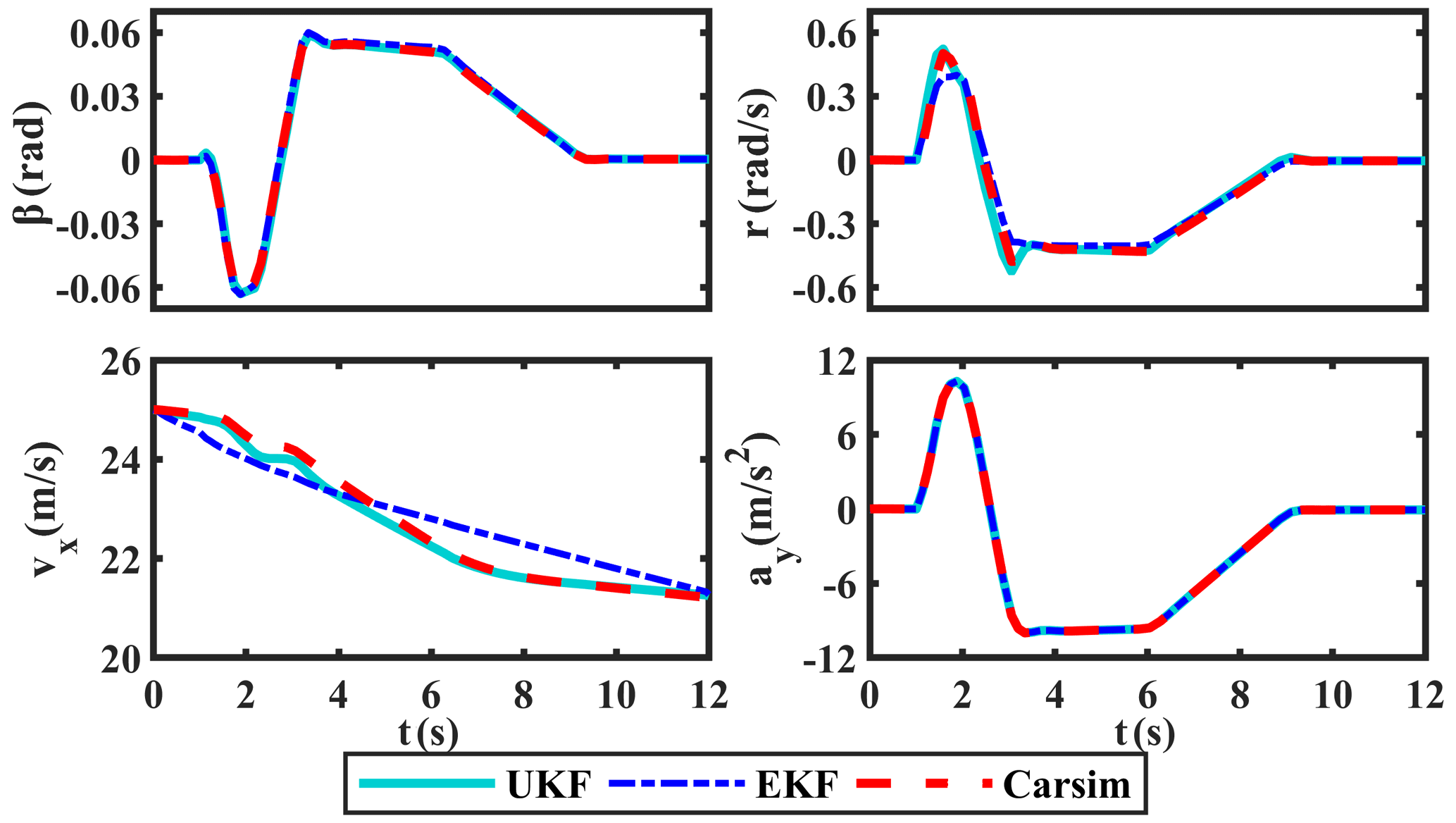
The sine manoeuver test is first carried out in the CarSim environment, and the simulation results of δ and a_x are shown in Fig. 5. Taking these estimates as pseudo-measured values and input values, we use the proposed UKF-based estimation method to estimate the required states. Simultaneously, the comparison curves of β, r, v_x, and a_y, along with their corresponding absolute and relative error curves, are provided in Figs. 6, 7, and 8, respectively.

Figure 5 The results of δ and a_x under the sine manoeuver test.

Figure 6 The estimated results of β, r, v_x, and a_y under the sine manoeuver test.

Figure 7 The absolute error curves of β, r, v_x, and a_y under the sine manoeuver test.

Figure 8 The relative error curves of β, r, v_x, and a_y under the sine manoeuver test.

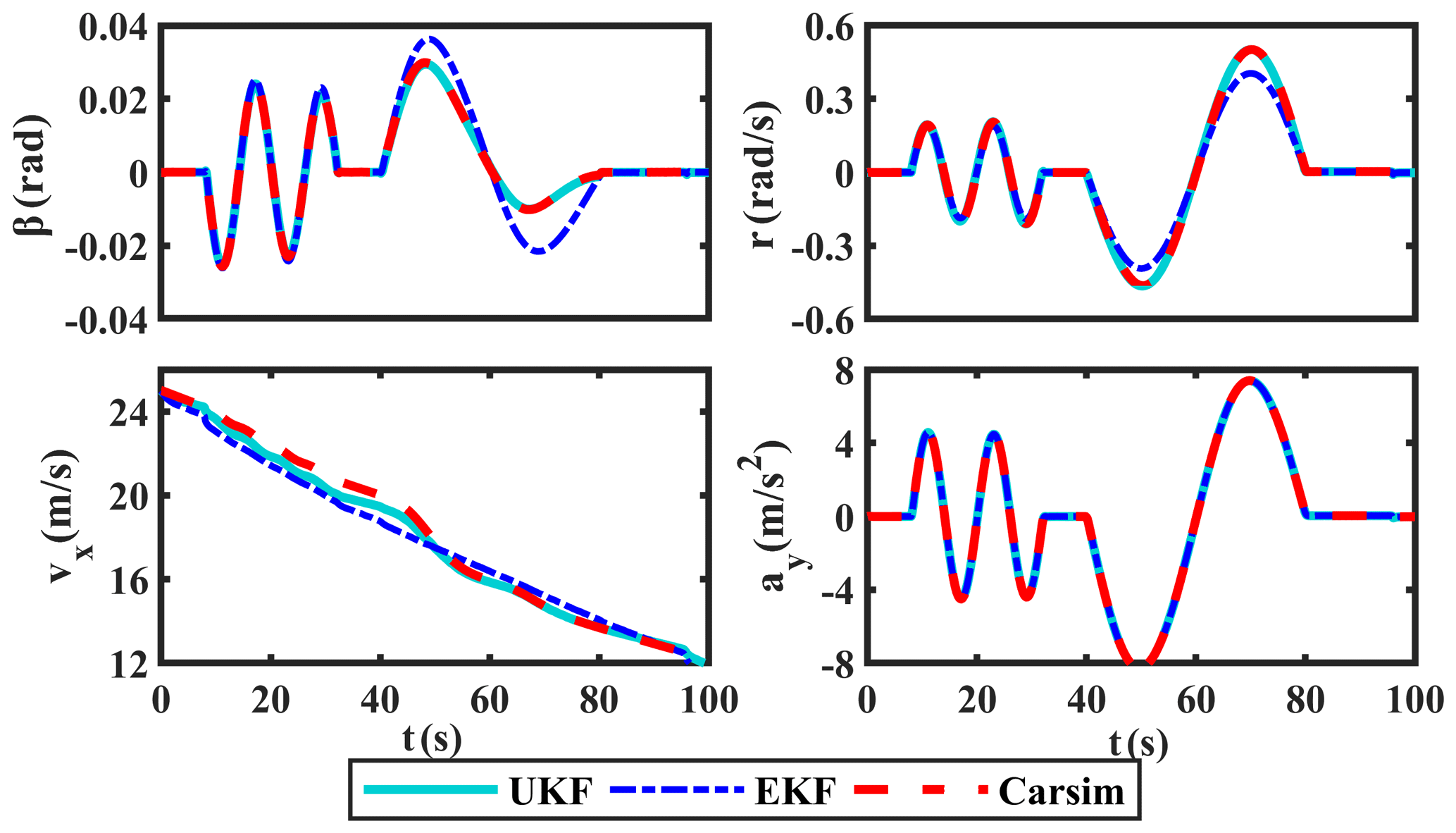
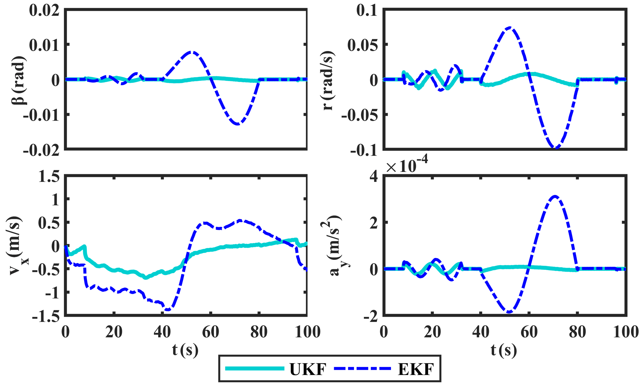
In terms of the results in Figs. 6, 7, and 8, the estimated values of UKF on β, r, v_x, and a_y are basically consistent with the measured values gotten by CarSim software and have smaller absolute errors than EKF. Among them, the relative errors of UKF on β, r, v_x, and a_y are basically kept below 3 %; only when the steering wheel angle reaches its maximum will the fluctuation of the relative errors be a little larger. In general, the relative errors of UKF are lower than EKF. Obviously, UKF has better estimation ability than EKF.

4.2 Fishhook manoeuver test

4.2.1 Case I

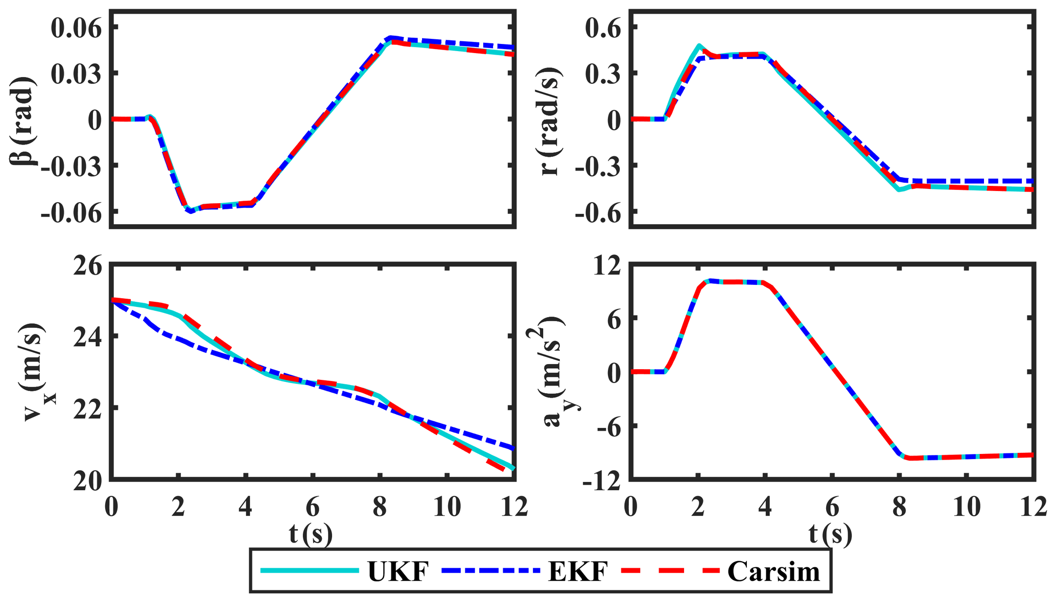
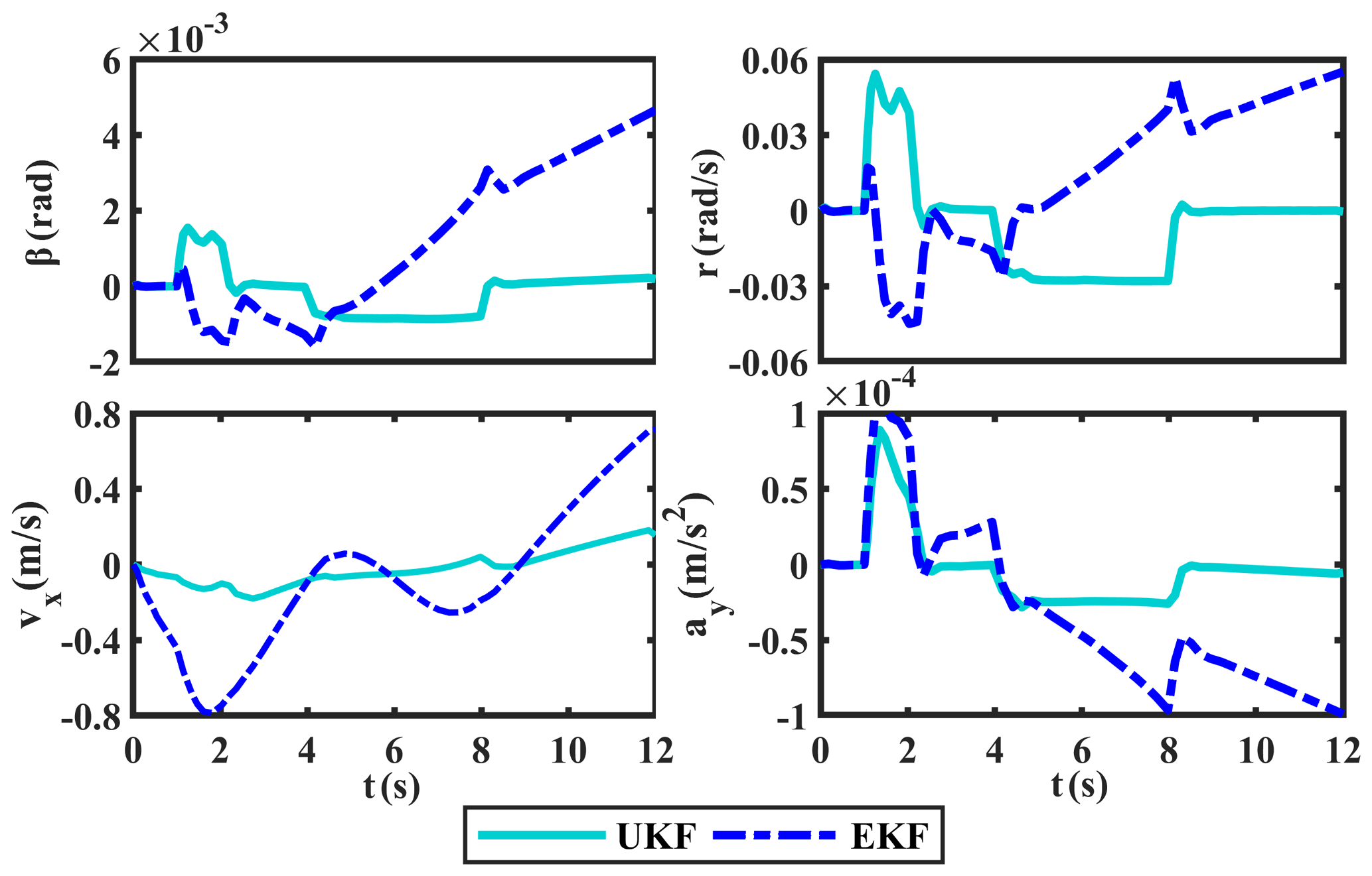
The similar simulations are conducted under the fishhook manoeuver test I scenario using CarSim software, and the obtained δ and a_x are shown in Fig. 9. Meanwhile, the comparison curves of β, r, v_x, and a_y, along with their corresponding absolute and relative error curves, are provided Figs. 10, 11, and 12, respectively.

In terms of Figs. 10, 11, and 12, there is also a high consistency in UKF between the estimated and measured values of β, r, v_x, and a_y under fishhook manoeuver test I. Especially the absolute error of v_x with UKF is far lower than that with EKF. Under the circumstance that the absolute error of EKF presents an increasing trend, the error curve of UKF is still relatively flat. Meanwhile, the relative errors of UKF on v_x and a_y are always kept below 3 %; only the relative errors of β and r are relatively high at 0 and 2 s, respectively, and later they also decrease to below 3 %, which indicates that the estimation results of the proposed UKF-based driving states estimation method have higher accuracy.

Figure 9 The obtained δ and a_x under fishhook manoeuver test I.

Figure 10 The estimated results of β, r, v_x, and a_y under fishhook manoeuver test I.

Figure 11 The absolute error curve of β, r, v_x, and a_y under fishhook manoeuver test I.

Figure 12 The relative error curve of β, r, v_x, and a_y under fishhook manoeuver test I.

Table 2 The MAPE of UKF on β, r, v_x, and a_y.

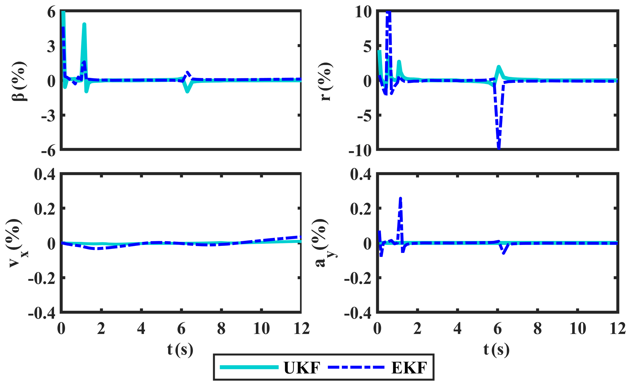
4.2.2 Case II

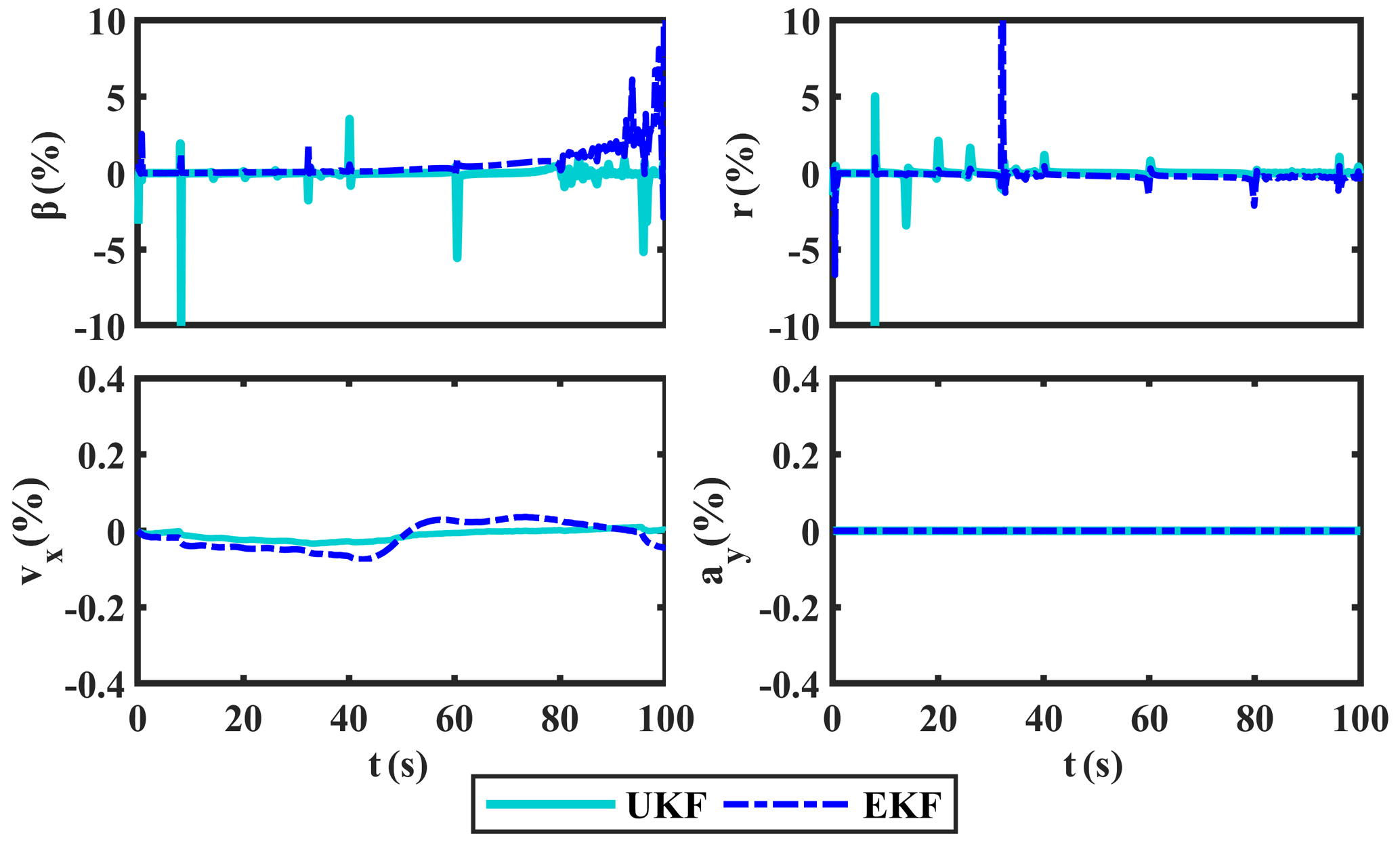
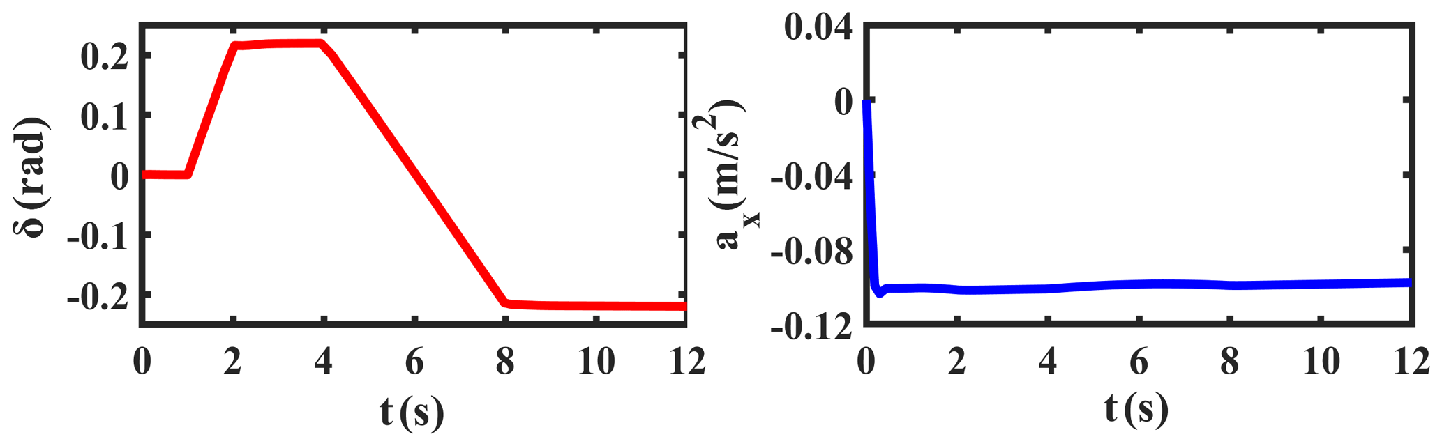
Similar to the simulation in Case I, the related simulations are carried out under fishhook manoeuver test II. The obtained results of δ and a_x are displayed in Fig. 13, which are used as the inputs to the UKF-based simulation model in the MATLAB/Simulink environment. Thus, the comparison curves of β, r, v_x, and a_y, along with their corresponding error curves, are displayed in Figs. 14, 15, and 16, respectively.

Figure 13 The obtained δ and a_x under fishhook manoeuver test II.

Figure 14 The estimated results of β, r, v_x, and a_y under fishhook manoeuver test II.

Figure 15 The absolute error curve of β, r, v_x, and a_y under fishhook manoeuver test II.

Figure 16 The relative error curve of β, r, v_x, and a_y under fishhook manoeuver test II.

Figure 17 The average error of the proposed UKF-based estimation method and traditional EKF.

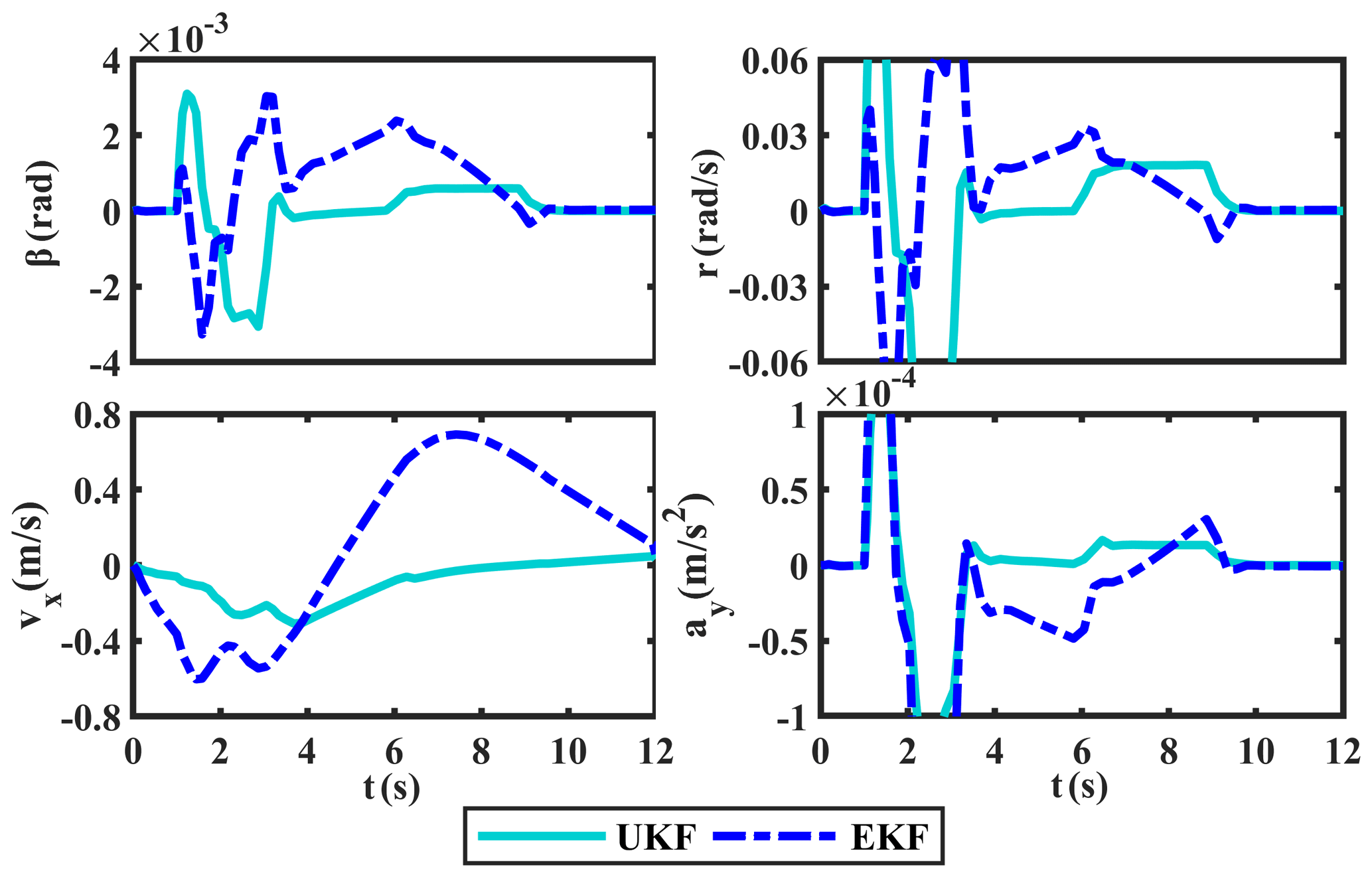
Like the situations in Case I, the proposed UKF-based vehicle estimation method still maintains a higher accuracy than EKF in Case II, and only the error of β and r at 2 and 10 s is relatively large. It is noted that the vehicle will be unstable at these two moments when steering quickly at a high speed. In other words, the working area of the tire is shifted, which weakens the axle cornering characteristic and changes the steering characteristic of the vehicle (Zhang et al., 2014), resulting in a larger error.

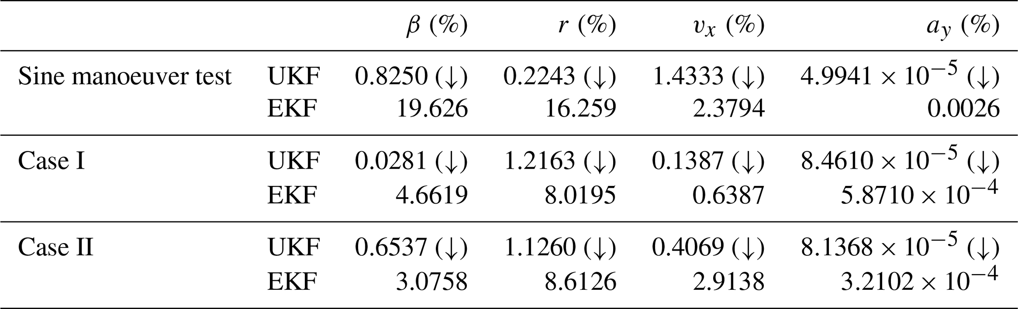
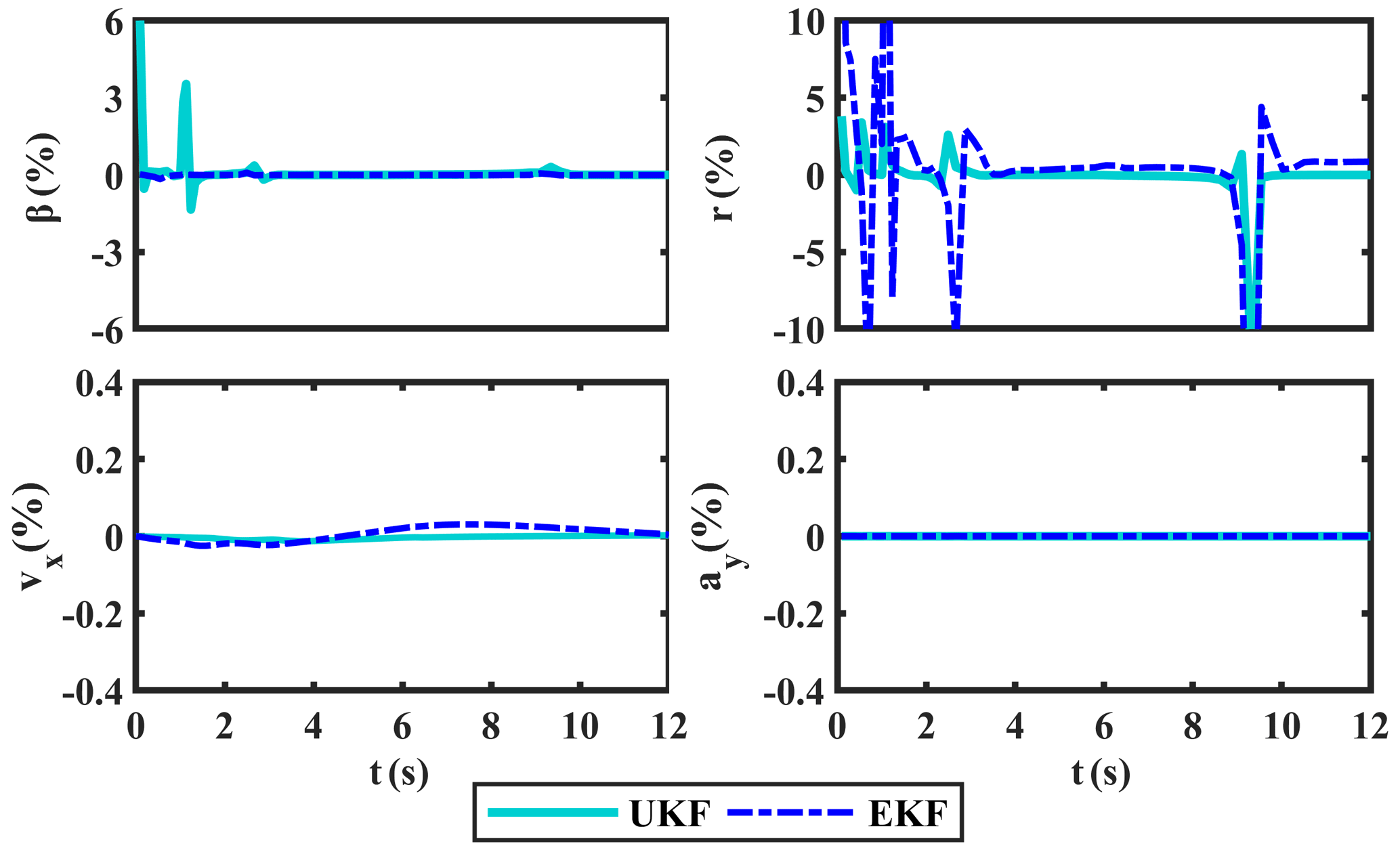
To further demonstrate the accuracy of the proposed UKF-based vehicle states estimation method, the mean absolute percentage error (MAPE) (Ma et al., 2016), a statistical index which can express the estimation error as a percentage, is given as below:

$$\begin{array}{}\text{(23)}& {\mathit{x}}_{\mathrm{MAPE}}={\displaystyle \frac{\mathrm{1}}{N}}\sum _{k=\mathrm{1}}^N\left|{\displaystyle \frac{{\mathit{x}}^{\ast }\left(k\right)-\widehat{\mathit{x}}\left(k\right)}{{\mathit{x}}^{\ast }\left(k\right)}}\right|,k=\mathrm{1},\mathrm{2},\mathrm{\dots },N,\end{array}$$

where x^∗(k) is the exact value of the vehicle state at moment k, which is the state value estimated by CarSim software in this paper; $\widehat{\mathit{x}}\left(k\right)$ is the estimated value of UKF at moment k, that is, the posterior state value obtained by Eq. (22); N is the number of state values of the vehicle.

The MAPE of UKF and EKF on β, r, v_x, and a_y under the sine manoeuver test, Case I, and Case II are shown in Table 2, and the average errors of the proposed UKF-based method and traditional EKF are displayed in Fig. 17.

As shown in Table 2, the MAPEs of UKF on β, r, and v_x are all around 1 % and lower than that of EKF under the three kinds of conditions, while the MAPE of a_y is so small that it can be ignored. In addition, the average error of the proposed UKF-based estimation method displayed in Fig. 17 was lower far from these of the EKF, which implies that the proposed UKF-based estimation method can keep a better overall accuracy than EKF when estimating the driving states of vehicles.

5 Conclusions and future work

In this paper, we proposed a type of UKF-based vehicle driving state estimation method with higher accuracy. First, a 3-DOFs vehicle dynamics model is established, and then a vehicle driving state estimation method is designed based on the UKF algorithm. Finally, by using CarSim and MATLAB/Simulink software, the co-simulation and validation are carried out to validate the accuracy of the proposed estimation method under the sinusoidal and fishhook conditions. Several highlights of this work are given below.

1. A complete UKF-based co-estimation method is proposed to predict the values of β, r, v_x, and a_y for a ground vehicle by combining CarSim and MATLAB/Simulink software.

2. Through the co-simulation and validation, we obtain that the average errors of β, r, v_x, and a_y with our proposed UKF-based estimation approach are, respectively, reduced by about 94 %, 92 %, 67 %, and 97 % in comparison with those with the EKF-based approach. The simulation results validate that the proposed co-estimation method can well predict the driving states of vehicles with higher accuracy.

In the future works, we would like to focus on the research of the adaptive UKF-based estimation method and try to use the adaptive algorithm to reduce the impacts of noise covariance on the accuracy of the desirable estimation method.

Appendix A

The state matrices of state-space Eq. (8):

$$\begin{array}{rl}& \mathbf{A}=\left[\begin{array}{lll}\frac{k_{\mathrm{1}}+k_{\mathrm{2}}}{m{v}_x}& \frac{a{k}_{\mathrm{1}}-b{k}_{\mathrm{2}}-m{v}_x^{\mathrm{2}}}{m{v}_x^{\mathrm{2}}}& \mathrm{0}\\ \frac{a{k}_{\mathrm{1}}-b{k}_{\mathrm{2}}}{I_z}& \frac{a^{\mathrm{2}}{k}_{\mathrm{1}}+b^{\mathrm{2}}{k}_{\mathrm{2}}}{I_z{v}_x}& \mathrm{0}\\ \mathrm{0}& \mathrm{0}& \mathit{\beta }r\end{array}\right],\\ & \mathbf{B}=\left[\begin{array}{ll}-\frac{k_{\mathrm{1}}}{m{v}_x}& \mathrm{0}\\ -\frac{a{k}_{\mathrm{1}}}{I_z}& \mathrm{0}\\ \mathrm{0}& \mathrm{1}\end{array}\right],\\ & \mathbf{C}=\left[\begin{array}{lll}\frac{k_{\mathrm{1}}+k_{\mathrm{2}}}{m}& \frac{a{k}_{\mathrm{1}}-b{k}_{\mathrm{2}}}{m{v}_x}& \mathrm{0}\end{array}\right],\\ & \mathbf{D}=\left[\begin{array}{ll}-\frac{k_{\mathrm{1}}}{m}& \mathrm{0}\end{array}\right].\end{array}$$