Design and analysis of mobile mechanism based on three-dimensional Hilbert curve

This paper introduces a mobile mechanism inspired by three-dimensional Hilbert curves, comprising the Hilbert first-order curve mobile mechanism (HFCM) and the second-order curve mobile mechanism (HSCM). The HFCM, a bipedal system, utilizes seven actuated telescopic joints to replicate the geometric expansion–contraction behaviour of the first-order Hilbert curve. Featuring an amoeba-like adaptive morphology, this mechanism demonstrates high manoeuvrability in confined environments such as narrow pipelines and rubble zones through sequential segment actuation. Stability analysis, kinematic modelling, and experimental validation confirmed its capabilities for static walking, rotational motion, and stair negotiation on planar surfaces. The HSCM, designed based on the second-order Hilbert curve, underwent comprehensive gait planning and dynamic stability evaluation. ADAMS simulations validated its planar translation and omni-directional rotation performance under uniform mass distribution. This research establishes a novel design framework for reconfigurable mechanisms, with future work focusing on developing higher-order Hilbert curve-based systems and exploring their applications in disaster response robotics.

1 Introduction

The design of the mechanism may be approached in a number of ways. One such method is to combine the regular geometric patterns found in mathematics as a basis for designing the mechanism to be made into a physical entity. This may then be actuated so that it has a variety of motions. Such a design may be analysed using spiral theory (Gogu, 2005), the centre of gravity offset method (COG) (Phipps et al., 2008), the zero moment method (ZMP) (Tian and Yao, 2015), etc. It is usual for this combined design to be classified into the following three types.

1. The design of planar mechanisms involves the combination of planar geometries, with the nodes of these mechanisms being designed as rotary joints and the edges or interior being designed as mobile joints. Sugiyama et al. (2005) utilized a circle as a reference to design a circular mechanism for crawling, with the shape of the external flexible crawler being controlled through the internal rigid structure to achieve mobility. Liu et al. (2012a) employed a triangle as a basis for the design of a new type of triangular mechanism, with the triangular shape being a fundamental element of the design. An analysis was conducted of in-plane linear walking and up-step movement. Subsequently, the steering function was realized through enhancement of the structure. Liu et al. (2012b) proposed a series of mobile 4R linkage mechanisms to accomplish rolling gait, utilizing the parallelogram as a template. These linkage mechanisms are capable of performing straight-line movement or turning movement. Wang et al. (2018) combined the ortho-five deformation with the circular ring and proposed a closed five-circle arc rod mechanism for the morphological rolling mechanism. Yao et al. designed a hexagonal mechanism based on the hexagonal shape with multiple deformations that can be rolled in a manner modelled on a track. Hao et al. (2020) designed two single-degree-of-freedom rolling extensible mobile linkage mechanisms whose shapes can be considered as originating from hexagonal and octagonal shapes. This combined design retains the dimensions of plane geometry, thereby imposing limitations on the direction of motion when moving on a plane.

2. The integration of plane geometry in the design of spatial mechanisms: the combination of multiple plane geometries results in the formation of a spatial geometric pattern, wherein the nodes of the plane geometries are engineered as rotary joints. Böhm et al. (2016) proposed a mobile mechanism based on a tensile monolithic structure, in which two rigidly disconnected bending members of the system can be regarded as two vertically arranged semi-circles connected by multiple tensile members. These members are capable of movement in a specific direction, facilitated by the action of internal mass. Semi-circular rings, connected by several tensile members, can be moved in a certain direction under the action of internal mass. Sugiyama et al. (2005) arranged three rings in a vertical configuration with respect to each other and proposed a spherical soft mechanism that is capable of crawling and jumping. Wei et al. (2019) arranged three octagons in a vertical configuration with respect to each other in a similar way to achieve rolling motion. Tian et al. (2015) connected eight identical isosceles right triangles with rotary joints to form a rolling eight-bar linkage mechanism. Eight identical equilateral triangles are connected with rotary joints in order to create a deformable polyhedral mechanism. These two designs can achieve various forms of rolling. Liu et al. (2012c) designed a basic biped RCCR mechanism, which can be structurally viewed as a smaller square inside a square, through the two squares' sequentially leaving and landing on the ground to achieve a walking gait.

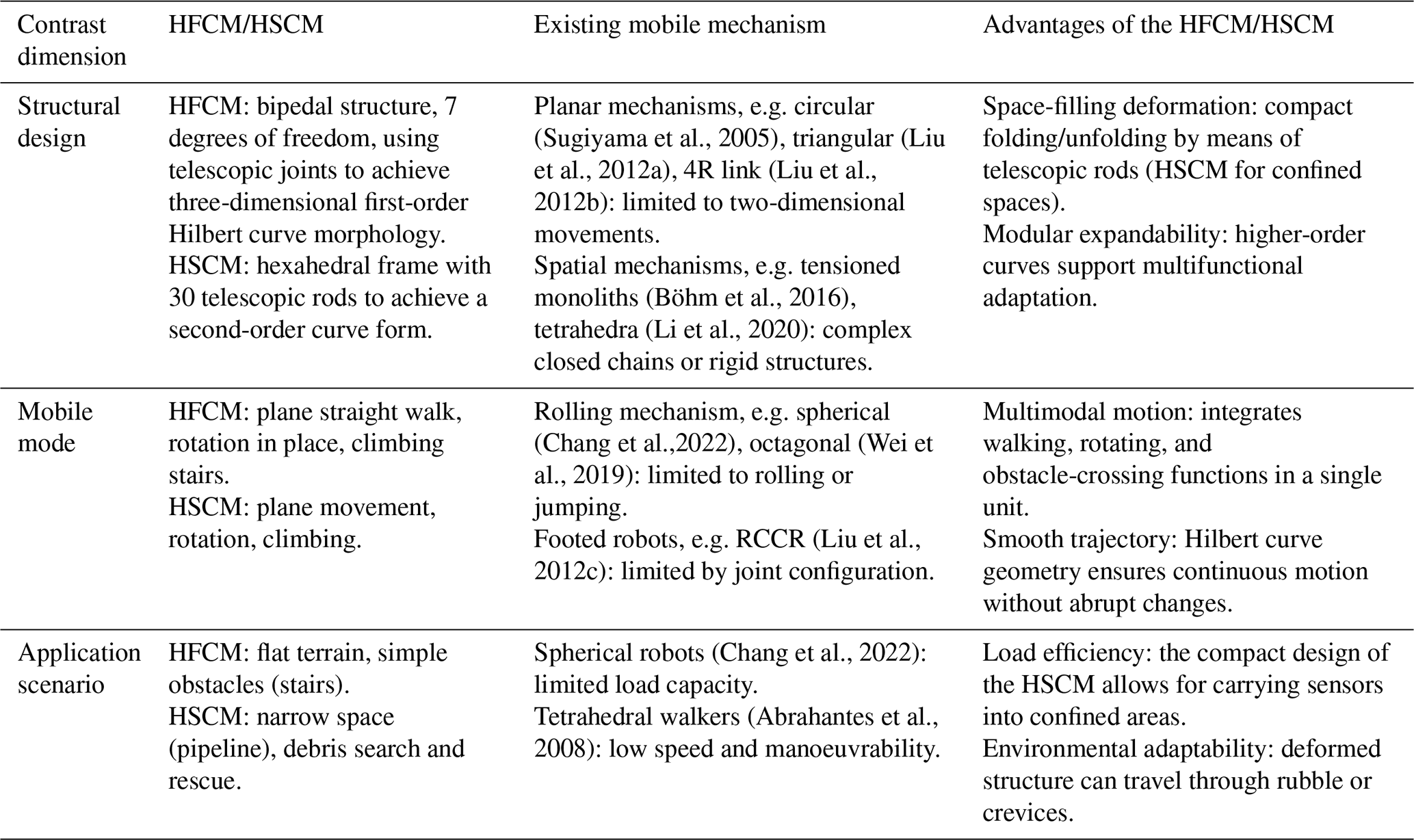
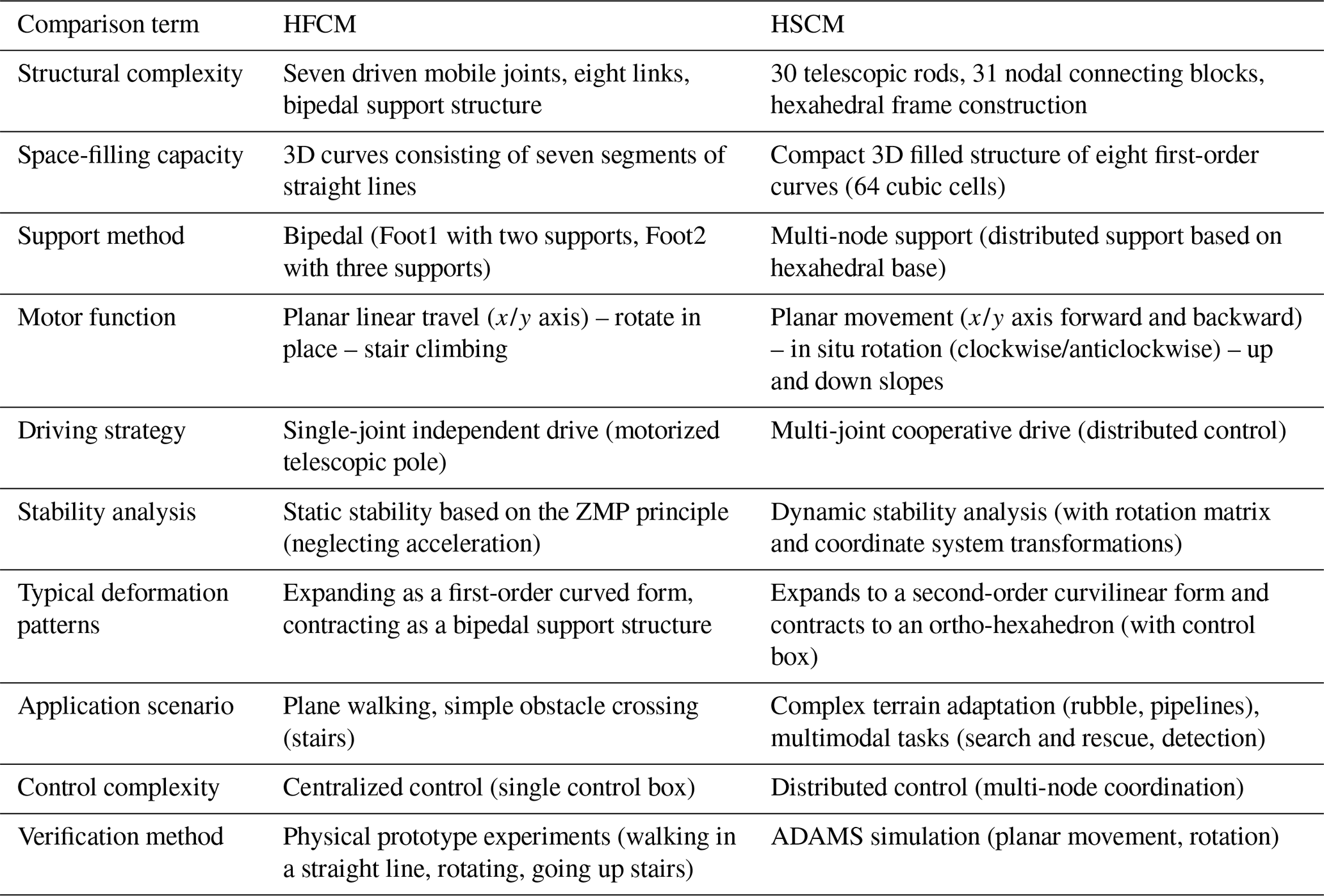
3. The design of spatial mechanisms by combining spatial geometry: spatial geometry is integrated into the structural design by establishing rotational joints, moving joints, and actuation. Kilin et al. (2015) conceived a combined spherical mechanism with a spherical shape, and by moving the centre of mass and altering the momentum of the internal gyroscope, it can attain an arbitrary trajectory motion along the plane. Chang et al. (2022) divided the spherical surface into two hemispherical surfaces and set up a jumping structure in the middle, with the hemispherical surface being designed as a wheel, which can achieve rotation, rolling, and jumping motion. Bian et al. (2024) proposed a novel wheeled rolling robot composed of a planar 3-RRR parallel mechanism and spoke-type variable-diameter wheels and validated its ability to perform linear rolling, turning, and small-angle climbing through kinematic/dynamic modelling, simulation, and prototype experiments. Building on the theoretical foundation of the planar 6R single-loop chain, Liu et al. (2024) developed a 4–5R rolling mechanism and introduced a unified gait strategy expression along with evaluation indices, achieving both high-speed and stable rolling gaits through simulation and physical validation. More recently, Xun et al. (2025) designed an anti-parallelogram ring four-array rolling mechanism capable of flexibly switching among parallelogram rolling, anti-parallelogram tumbling, and spherical rolling gaits, with its feasibility confirmed through dynamic analysis and experiments. Mahboubi et al. (2013) mixed the structure of spherical and common quadrupedal mechanisms and proposed a new hybrid quadrupedal football-shaped mobile mechanism. Li et al. (2020) based their deformable tetrahedral rolling mechanism on a tetrahedron design, comprising four platforms and six URU chains. Building on this, Liu et al. (2020a) added four branching tetrahedra to design a new deployable tetrahedral mobile mechanism consisting of an eight-degree-of-freedom Sarrus link mechanism. Abrahantes et al. (2008) also designed a mechanism based on tetrahedra that can walk. Liu and Yao (2019) proposed a novel nine-degree-of-freedom series parallel hybrid worm mechanism by combining the worm's kinematic mechanism and the combinatorial properties of the series-parallel structure, which can be conceptualized as a tri-prism with deformation capability. Paul and Lipson (2005) combined the tensioning mechanism with the characteristics of tri-prisms and torsion quadrangles and designed a mechanism based on the tensioning of the whole body by three and four strut prisms, where the mechanism can move in a straight line under the motion of the tensioning structure. Liu et al. (2020b) proposed and analysed a novel spring-containing tensioned integral mechanism by combining the tensioning mechanism with rhombohedrons. Cui et al. (2022) proposed a tensioned integral leg quadrupedal mechanism by designing such a mechanism as the foot of a quadrupedal mechanism. Tian et al. (2017) designed a reconfigurable multimodal mobile parallel mechanism, whose structure can be considered as setting the rotational joints at the vertices of a rectangular body and at the centres of the prismatic edges. Ding and Yao (2017) proposed a type of expandable cubes (E-cubes) that can achieve a variety of mobility functions by combining multiple E-cubes into different configurations. This was achieved by combining the mobile joints with a square body. Ding and Yao (2014) set a large number of mobile joints on a square structure so that the square can achieve rolling motion. A comparison of HFCM/HSCM with a similar mechanism as the above is shown in Table 2.

The majority of mechanisms conceived under these three categories are closed-chain mechanisms and shorter open-chain mechanisms with predominantly rolling motion. However, in our design, the longer open-chain mechanism is employed. In this paper, we propose a moving mechanism based on Hilbert curve features. The primary advantage of this mechanism is its ability to move and rotate smoothly along a straight line on a flat surface while requiring a relatively simple control strategy. The three-dimensional (3D) Hilbert curve, as a representative space-filling curve, has attracted increasing attention in the robotics field due to its advantages in locality preservation and spatial coverage. In path planning, it enables the generation of continuous and uniformly distributed trajectories, making it suitable for coverage tasks such as inspection, spraying, and cleaning. Compared with conventional approaches, it reduces the number of turns and improves motion efficiency. In 3D environment modelling and perception, the 3D Hilbert curve has been utilized for point cloud ordering and sparse sampling, thereby accelerating voxel partitioning and data retrieval and enhancing the real-time performance of SLAM and 3D reconstruction. Moreover, its data-mapping and partitioning capabilities have shown potential for multi-robot systems, particularly in workload distribution and storage optimization. In addition, researchers have explored its role in workspace division and cooperative task allocation to improve operational uniformity and system-level efficiency.In computational modelling and simulation, 3D Hilbert curves offer advantages in terms of efficient data management and visualization. For example, in the context of 3D city modelling, 3D Hilbert space-filling curves (HSFCs) can significantly accelerate spatial queries by providing a linearized representation of complex 3D data, which is especially useful for applications in urban planning and photogrammetry (Ujang et al., 2014). Similarly, in volumetric mesh visualization, an adaptive strategy based on extending the autonomous leaves graph to 3D, potentially leveraging principles akin to Hilbert curves, can reduce the computational cost of constructing and visualizing complex volumetric data generated from numerical simulations (Robaina et al., 2010). The Hilbert curve also aids in the visual comparison of 3D volumes by linearizing them into 1D Hilbert line plots, which can reveal subtle differences in ensembles of 3D data, as shown in applications such as medical imaging or materials science (Weissenbock et al., 2018).

Despite these promising applications, several challenges remain. First, the construction of 3D Hilbert curves is computationally complex, and high-order curves impose significant overhead on real-time generation and embedded systems. Second, the inherent sharp turns within Hilbert-based trajectories often conflict with the kinematic and dynamic constraints of robots, limiting efficiency and feasibility in practice. Third, the curve is naturally suited to regular cubic spaces, while real robotic environments are typically irregular and dynamically changing. Integrating 3D Hilbert curves with real-time obstacle avoidance and dynamic re-planning thus remains an open issue. Furthermore, in multi-robot collaboration, task division and trajectory scheduling based on Hilbert curves have yet to fully resolve conflicts and ensure fairness.

Overall, research on 3D Hilbert curves in robotics is of significant value and importance. On the one hand, it provides a mathematically elegant and computationally efficient approach for addressing coverage, data organization, and task allocation problems. On the other hand, it offers a unifying framework that bridges geometric theory with robotic motion planning and intelligent decision-making. Future investigations into adaptive curve optimization, integration with dynamic perception, and multi-robot coordination are therefore not only necessary for overcoming current limitations but also critical for unlocking the full potential of Hilbert-curve-based methods in advancing robotic intelligence and autonomy. Integrating the three-dimensional Hilbert curve with mechanism design provides a novel perspective for subsequent robotic design.

The contributions of this paper are as follows:

1. A novel design concept integrating the spatial properties of mathematical curves with the design of mechanical mechanisms is introduced.

2. A first-order and second-order curve moving mechanism based on the characteristics of Hilbert curves is proposed. This mechanism exhibits a variety of moving functions.

The paper is organized as follows: Sect. 2 details the design of the mechanism; Sect. 3 presents the stability analysis of the first-order and second-order mechanisms and the motion analysis of the first-order mechanism; Sect. 4 presents the simulation analysis; Sect. 5 shows the experiments on the first-order prototype; and Sect. 6 offers a summary and an outlook for future work.

2 Design method

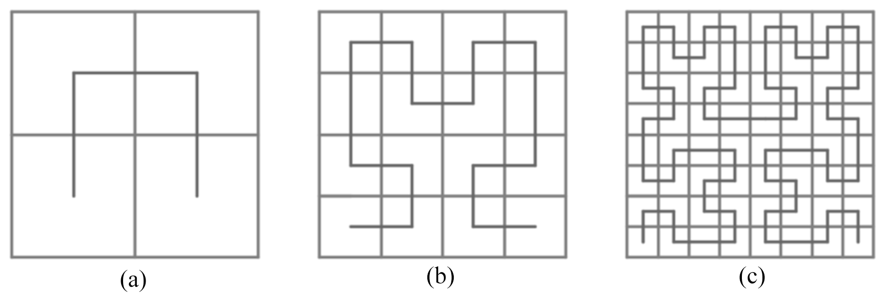
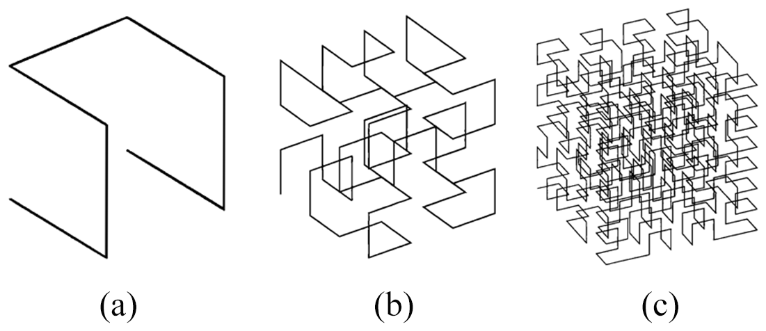
The three-dimensional (3D) Hilbert curve originates from the Hilbert curve proposed by the German mathematician David Hilbert in 1891 (see Fig. 1), which is a fractal curve capable of filling a two-dimensional square. As a natural extension, the 3D Hilbert curve maps a one-dimensional sequence onto three-dimensional space through a recursive construction, thereby achieving space-filling within a cubic domain; see Fig. 2 (Chen et al., 2022).

Figure 1 Hilbert curve. (a) First order, (b) second order, (c) third order.

Figure 2 3D Hilbert curve. (a) First order, (b) second order, (c) third order.

2.1 Design of HFCM

The Hilbert first-order curve moving mechanism (HFCM) has been designed based on three-dimensional Hilbert first-order curves, which exhibit a variety of spatial types (Zhang and Kamata, 2006). The HFCM has been designed with the spatial characteristics of the type of Fig. 2, which is a bipedal mechanism with a three-dimensional Hilbert first-order curve configuration. The three-dimensional Hilbert first-order curve consists of seven straight lines and six folds. The telescoping of the seven straight lines in the curve is realized by seven moving joints with actuators, as illustrated in Fig. 3c. Utilizing the motorized telescopic rods as moving joints with actuation enables them to function as reversible unfolding pillars. The adjustment of the position of the electric telescopic rod is conducted in accordance with the configuration depicted in Fig. 3c, with the objective of enhancing the compactness of the overall structure, reducing its dimensions, minimizing its weight, and aligning the spatial characteristics of the HFCM with those of the three-dimensional Hilbert first-order curve. The addition of linear bearings and guide shafts serves to enhance the strength and precision of the mechanism whilst concomitantly reducing the influence generated by gravity, as illustrated in Fig. 3d. The eight nodes are labelled A, B, C, D, E, F, G, and H, and the configuration is illustrated in Fig. 3a and b. Between points A and B, there are two rods connected by a mobile joint with a travel of Δl. The assembly of points B and C, C and D, D and E, E and F, F and G, and G and H is identical. The structure of Foot1 consists of a rod between points A and B and two support structures fixed below. The second foot (Foot2) consists of a rod between points G and H and three support structures fixed below. The support structure consists of a support rod and a base plate in contact with the ground. Seven mobile joints made of rods are connected to each other at the first point. Thus, the HFCM is a spatial open-chain mechanism with eight rods and seven moving joints. In the following, the foot containing points A and B is designated Foot1, and the foot containing points G to H is designated Foot2.

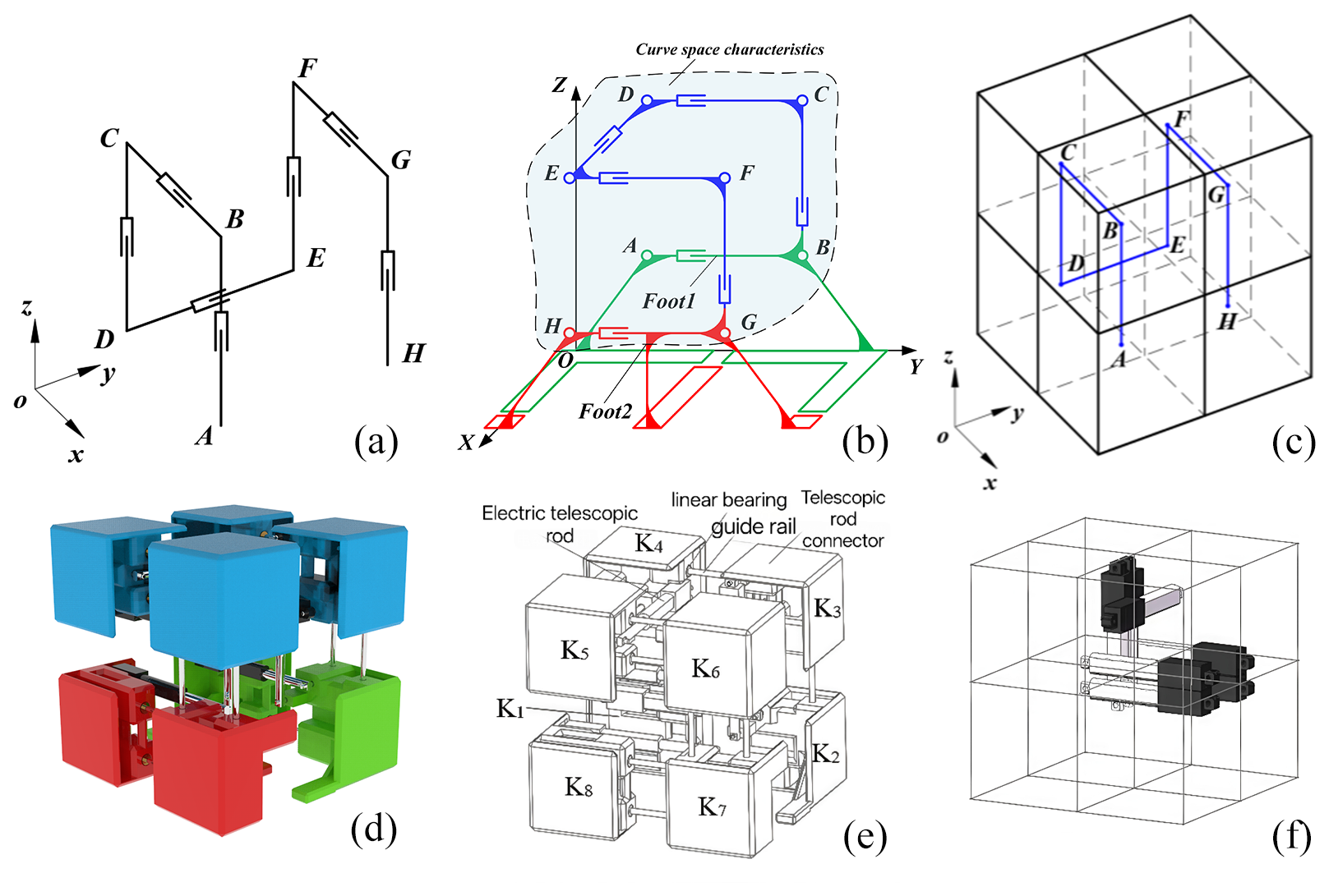
Figure 3 (a) Settings for first-order curve movement joints. (b) Schematic diagram of the mobile drive setup. (c) Simplified scheme of HFCM. (d) Diagram of 3D model. (e) 3D model. (f) Axonometric drawing.

2.2 HFCM's principle of mobility

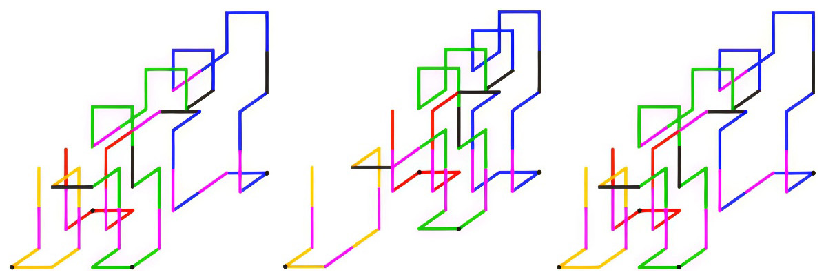
In light of the gravitational forces at play, the focus is narrowed to the study of the HFCM's degrees of freedom along the x and y axes within the two-dimensional plane. The underlying principle governing the act of walking is elucidated as follows. For the x-axis direction, consider curve A₀B₀C₀D₀E₀F₀G₀H₀ shown in Fig. 4a. a_i is the centre of mass of the eight connectors. Figure 4a shows the initial stance. If Foot1 is the stance foot, B₀C₀ and D₀E₀ are expanded to change the curve to A₀B₀C₁D₁E₁F₁G₁H₁. As shown in Fig. 4b, Foot2 lifts, and the EFGH part of the curve is shifted positively along the x axis by Δl. Then, expanding F₁G₁, to change the curve configuration to A₀B₀C₁D₁E₁F₁G₂H₂, Foot2 falls. Similarly, Foot2 is the standing foot. The configuration curve A₀B₀C₁D₁E₁F₁G₂H₂ is transformed into a curve A₁B₁C₂D₂E₁F₁G₂H₂ by sequentially contracting or expanding the straight lines in the curve. Lifting Foot1, the ABCD part of the curve is shifted positively along the x axis by Δl. Then, the configuration i changed to A₂B₂C₂D₂E₁F₁G₂H₂. As demonstrated in Fig. 4f, at this particular point, the curve exhibits the same attitude as the initial curve. The curve as a whole is shifted positively along the x axis by Δl. It is evident that by repeating procedures (b) to (e) in Fig. 4, the curve can be continuously shifted positively along the x axis. In a similar manner, by inverting the trajectory of a curve that is progressing in a positive direction along the x axis, the curve can be repeatedly shifted in a negative direction along the same axis.

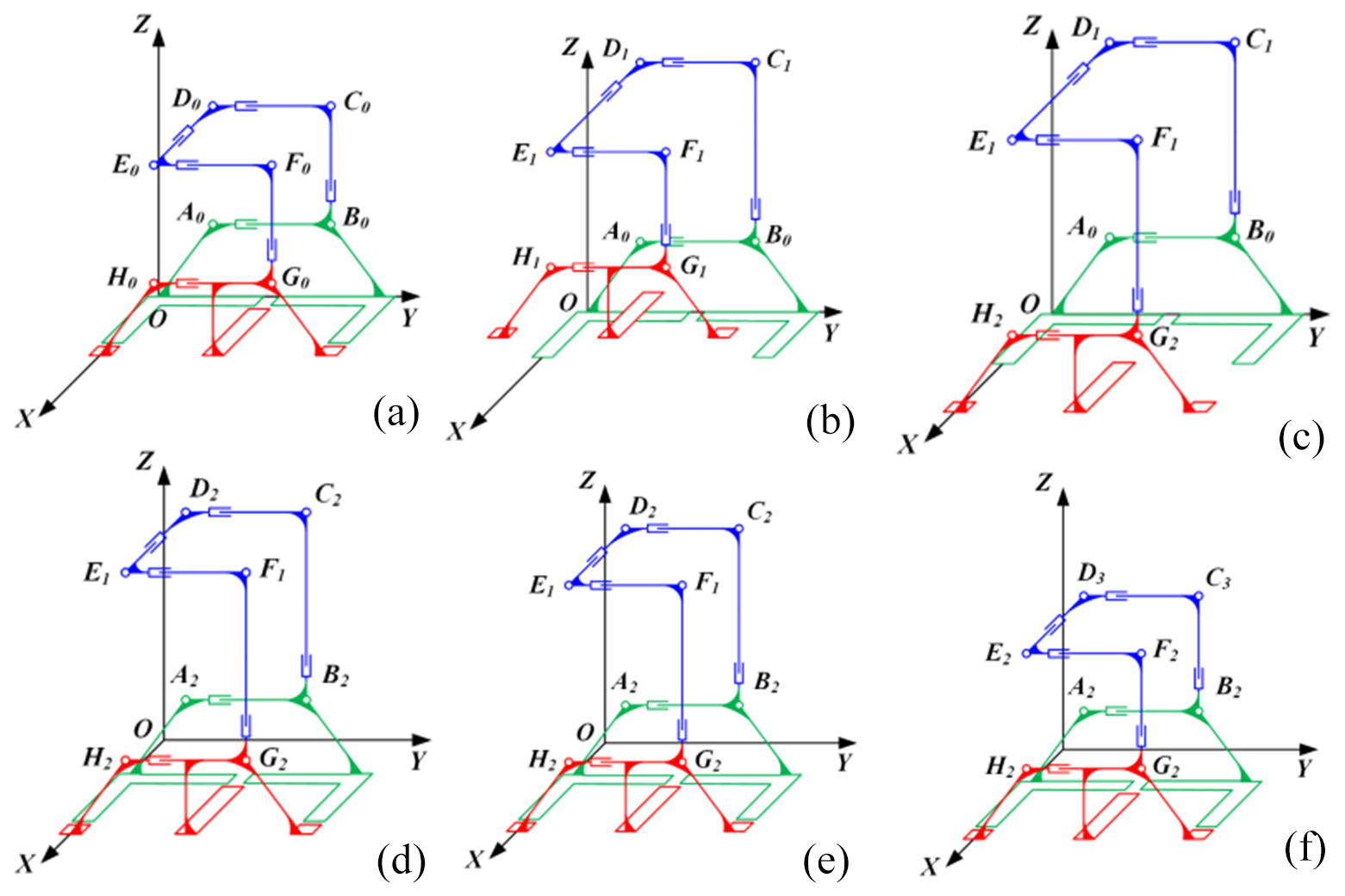
Figure 4 Gait diagram of forward movement along the x axis. (a) Gait 1, (b) gait 2, (c) gait 3, (d) gait 4, (e) gait 5, (f) gait 6.

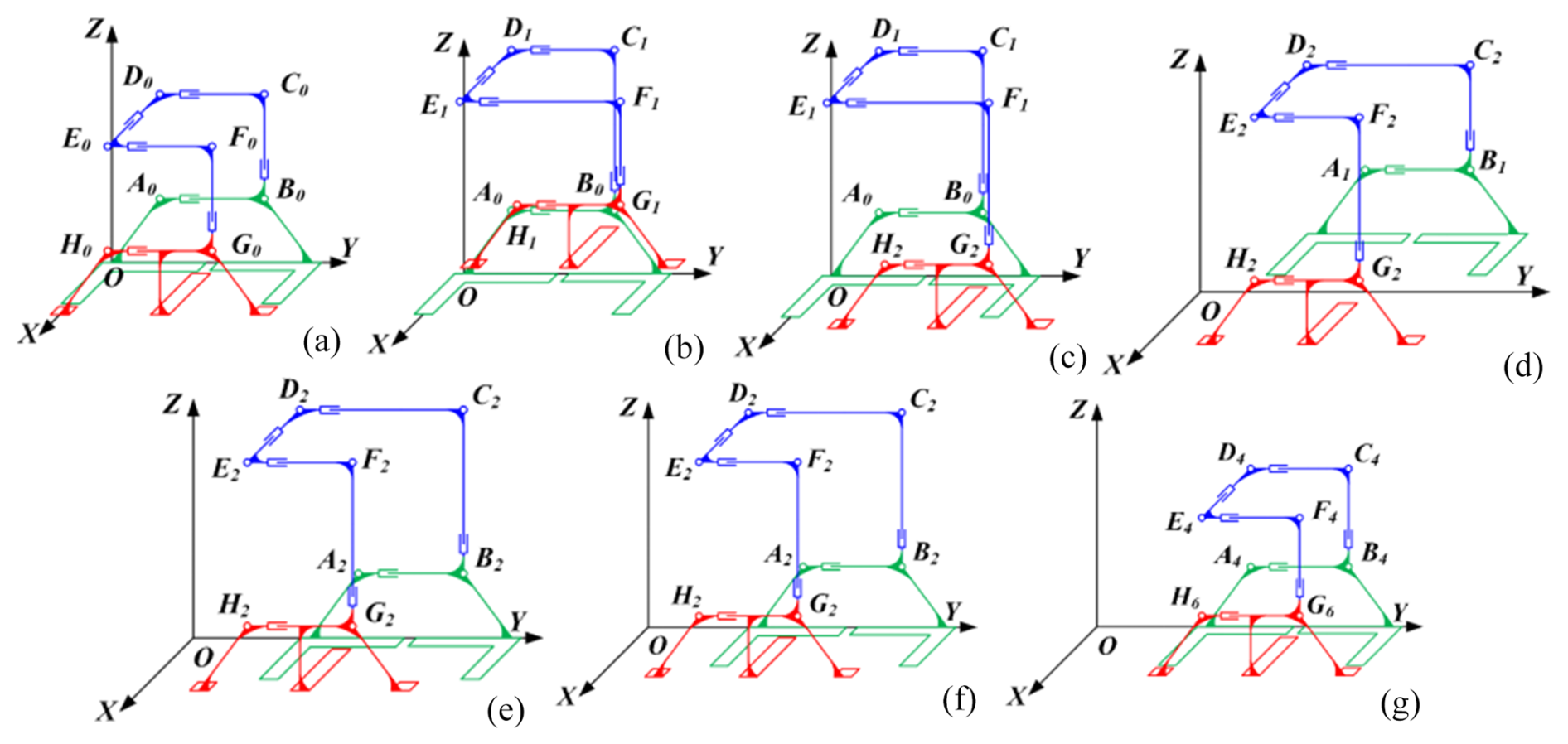
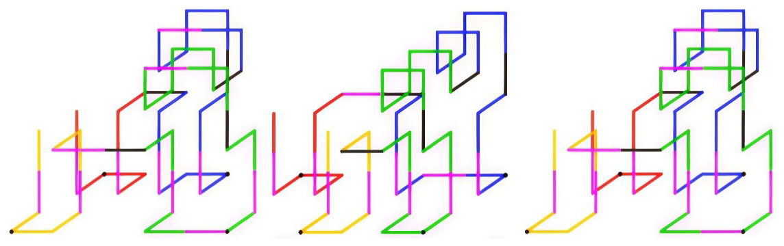
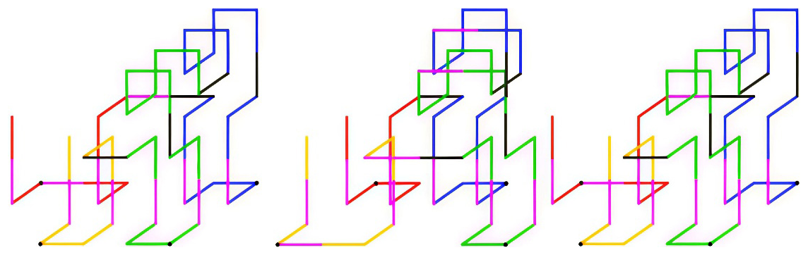
Figure 5 Gait diagram for forward movement along the y axis. (a) Gait 1, (b) gait 2, (c) gait 3, (d) gait 4, (e) gait 5, (f) gait 6, (g) gait 7.

In Fig. 5, the curve is A₀B₀C₀D₀E₀F₀G₀H₀. Figure 5a shows the initial attitude. When Foot1 is the standing foot, B₀C₀ and E₀F₀ expand to change the configuration to curve A₀B₀C₁D₁E₁F₁G₁H₁ to lift Foot2. Then, changing the configuration to curve A₀B₀C₁D₁E₁F₁G₂H₂, Foot2 falls. At this point, Foot2 is the standing foot, and then E₁F₁ and B₀C₁ contract, expand, and lift Foot1. Then, the configuration is changed to curve A₂B₂C₂D₂E₂F₂G₂H₂. At this point, the curve as a whole advances along the y axis by Δl. Then, the straight lines in the curve are contracted or expanded in sequence, turning the curve into curve A₄B₄C₃D₂E₂F₂G₃H₃, and Foot1 falls. Subsequently, the configuration is to be altered to A₂B₂C₂D₂E₂F₂G₃H₃, with Foot2 then being elevated. Finally, the configuration is changed to A₂B₂C₃D₃E₃F₃G₄H₄, as illustrated in Fig. 5g. When Foot2 falls to the ground, the curve has the same attitude as the initial curve. At this juncture, the curve is shifted positively along the y axis by 2Δl. By repeating procedures (b) to (f) illustrated in Fig. 5, the curve can be shifted positively along the y axis in a continuous manner.

Conversely, the curve can be continuously moved in the negative direction along the y axis by reversing the configuration of the curve's gait in the positive direction along the y axis.

2.3 Design of HSCM

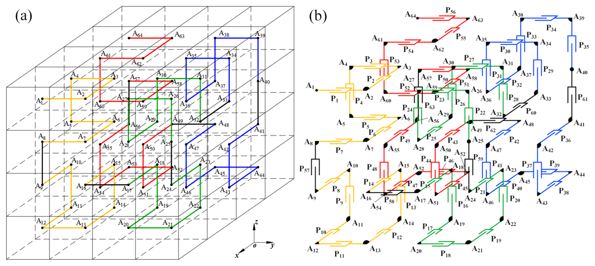
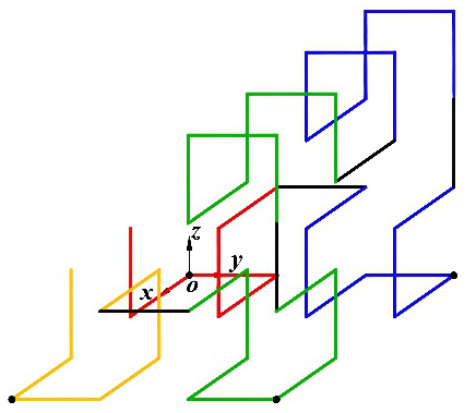
The three-dimensional Hilbert second-order curve depicted in Fig. 6a comprises eight first-order curves, which are interconnected by 63 straight segments of equal length. As demonstrated in Fig. 6b, the second-order curves can be arranged in a more compact configuration within the three-dimensional square space. The points A₁–A₆₄ represent the centres of 64 small squares, which are arranged in a stacked configuration to form a large square, and they also serve as the nodes of the second-order curves, respectively.

Figure 6 (a) 3D Hilbert second-order curve. (b) Mobile driver configuration diagram.

Table 1 HSCM base gait.

Table 2 Mechanism comparison.

The Hilbert second-order curvilinear moving mechanism (HSCM) necessitates a minimum of 30 telescopic rods, the corresponding positions of which are delineated in Fig. 7a. The red thick solid line signifies the requirement for a telescopic rod at that specific position. Leveraging this data, the structural design of the second-order moving mechanism is executed as follows:

1. The square space that the second-order curvilinear moving mechanism occupies is designed as the shape of the mechanism itself.

2. It is important to note that components A₁–A₁₀ and A₅₅–A₆₄ are exclusively implicated in the inverted reset motion. Consequently, the geometric characteristics of these components are streamlined in the structural design by eliminating components A₅–A₁₀ and A₅₅–A₆₀ and establishing direct connections between components A₅A₁₀ and A₅₅A₆₀ via straight lines, as illustrated in Fig. 7b.

3. The curved node part should be designed as a node connector, with 30 pushrods set between the connectors and combined with each other if no pushrods are set between the neighbouring connections and designed as one connector. Given that the inner part of the mechanism is a tandem mechanism, it is also necessary to add a guide rail structure similar to the first-order curve mechanism to increase the structural strength.

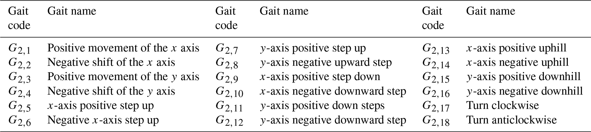
The three-dimensional diagram illustrating the structure of the second-order curve mechanism is presented in Fig. 8a and b. Figure 8a depicts the state in which the mechanism is fully expanded, exhibiting the spatial characteristics of the second-order curve. The second-order curve mechanism consists of 31 node connecting blocks N_i (i=1, 2, …, 31). The state of complete contraction of the mechanism is illustrated in Fig. 8b, where the mechanism adopts a positive six-sided configuration comprising 30 telescopic drives, guide rails, and control boxes. The guide rails are composed of metal rods and linear bearings, with the node connecting blocks positioned in groups of four between the guide rails to enhance the structural integrity of the mechanism. The control boxes are situated within the first and last node connecting blocks of the mechanism, serving as storage for the control board. The control box is located in the first and last node blocks of the mechanism and is used to store the necessary electronic components, such as control boards, actuators, and batteries. The basic gait for designing the HSCM is shown in Table 1.

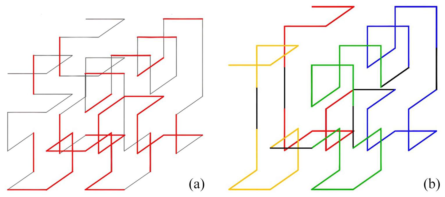
Figure 7 (a) Second-order curve expansion rod setting position diagram. (b) Spatial feature graph based on the second-order curve mechanism.

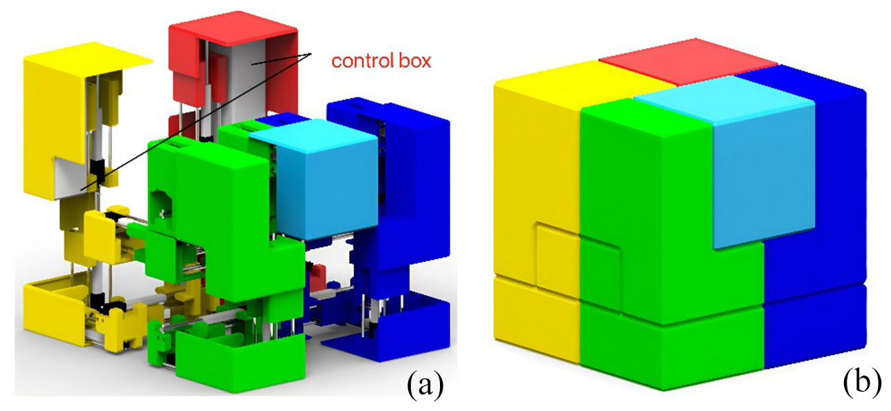
Figure 8 (a) 3D view of the structure of the second-order curvilinear mechanism (fully expanded). (b) 3D view of the structure of the second-order curvilinear mechanism (fully contracted).

Figure 9 Schematic diagram of the initial state of planar walking.

2.4 HSCM gait design

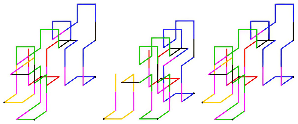
The initial state of planar walking is illustrated in Fig. 9. By executing the gait planning of G_2,1 and G_2,3 in reverse, the G_2,2 and G_2,4 gait can be derived. Additionally, due to the high symmetry of the lower part of the residual curve, G_2,2 and G_2,4 can also be derived by setting G_2,1 and G_2,3 symmetrically, respectively. In this study, symmetry is employed for the planning, and the planar walking gait planning is depicted in Figs. 10 to 13. As illustrated in Figs. 10 through 13, the subsequent gaits of G_2,5 and G_2,18 exhibit symmetry. Consequently, it is sufficient to plan the various types of motion along the x-axis positive, y-axis positive, and clockwise motion. Subsequently, the setup should be mirrored, and minor adjustments should be made to derive the x-axis negative, y-axis negative, and anticlockwise motion. A comparison of HFCM and HSCM as above is shown in Table 3.

Figure 10 Schematic representation of the expansion and contraction of G_2,1.

Figure 11 Schematic representation of the expansion and contraction of G_2,2.

Figure 12 Schematic representation of the expansion and contraction of G_2,3.

Figure 13 Schematic diagram of the expansion of G_2,4.

Table 3 Differences between HFCM and HSCM.

3 Stability and kinematic analysis

3.1 Static stability analysis

The zero moment point (ZMP) is a key indicator that the robot remains statically stable and needs to ensure that it is located within the support area of the supporting foot. The area of support is determined by the area of the soleplate at the end of the foot.

Table 4 The rotation angle of step j in G_2,13–G_2,16.

In order to guarantee the stability of the HFCM during operation, the position of the ZMP must be calculated using the zero moment point (ZMP) principle. The conditions for stable movement of the HFCM are as follows: the ZMP must be within the support area of Foot1 and Foot2. The following equations comprise the ZMP calculation:

$$\begin{array}{}\text{(1)}& \left\{\begin{array}{l}{x}_{\mathrm{ZMP}}=\frac{\left[\sum _{i=\mathrm{1}}^n{m}_i\left({\ddot{z}}_i+g_z\right)x_i-\sum _{i=\mathrm{1}}^n{m}_i{\ddot{x}}_i{z}_i-{\left(\sum _{i=\mathrm{0}}^n{J}_i{\mathit{\alpha }}_i\right)}_y\right]}{\sum _{i=\mathrm{1}}^n{m}_i\left({\ddot{z}}_i+g_z\right)}\\ y_{\mathrm{ZMP}}=\frac{\left[\sum _{i=\mathrm{1}}^n{m}_i\left({\ddot{z}}_i+g_z\right)y_i-\sum _{i=\mathrm{1}}^n{m}_i{\ddot{y}}_i{z}_i-{\left(\sum _{i=\mathrm{0}}^n{J}_i{\mathit{\alpha }}_i\right)}_x\right]}{\sum _{i=\mathrm{1}}^n{m}_i\left({\ddot{z}}_i+g_z\right)}\end{array}\right..\end{array}$$

This HFCM travels in a straight line with static stability as it moves along the x and y axes; therefore, acceleration and angular acceleration are neglected, and the mass of each linkage is the same. The ZMP of the HFCM is calculated as follows:

$$\begin{array}{}\text{(2)}& \left\{\begin{array}{l}{x}_{\mathrm{ZMP}}=\frac{\left[\sum _{i=\mathrm{1}}^n{m}_i\left({\ddot{z}}_i+g_z\right)x_i-\sum _{i=\mathrm{1}}^n{m}_i{\ddot{x}}_i{z}_i-{\left(\sum _{i=\mathrm{0}}^n{J}_i{\mathit{\alpha }}_i\right)}_y\right]}{\sum _{i=\mathrm{1}}^n{m}_i\left({\ddot{z}}_i+g_z\right)}\\ y_{\mathrm{ZMP}}=\frac{\left[\sum _{i=\mathrm{1}}^n{m}_i\left({\ddot{z}}_i+g_z\right)y_i-\sum _{i=\mathrm{1}}^n{m}_i{\ddot{y}}_i{z}_i-{\left(\sum _{i=\mathrm{0}}^n{J}_i{\mathit{\alpha }}_i\right)}_x\right]}{\sum _{i=\mathrm{1}}^n{m}_i\left({\ddot{z}}_i+g_z\right)}\end{array}\right..\end{array}$$

When the HFCM moves along the x axis and y axis,

$$\begin{array}{}\text{(3)}& \left\{\begin{array}{l}{x}_{\mathrm{ZMP}}=\frac{x_A+x_B+x_C+x_D+x_E+x_F+x_G+x_H}{\mathrm{8}}\\ y_{\mathrm{ZMP}}=\frac{y_A+y_B+y_C+y_D+y_E+y_F+y_G+y_H}{\mathrm{8}}\end{array}\right..\end{array}$$

In order to maintain static stability, it is necessary that the ZMP be located within the support area. When Foot1 is designated as the support foot, the support region is generated by the two base plates contained within Foot1. In order for this to be satisfied, the following conditions must be met:

$$\begin{array}{}\text{(4)}& x_{h\mathrm{1}}<x_{\mathrm{ZMP}}<x_{k\mathrm{1}}{y}_{h\mathrm{1}}-d_{\mathrm{1}}/\mathrm{2}<y_{\mathrm{ZMP}}<y_{h\mathrm{2}}+d_{\mathrm{1}}/\mathrm{2}.\end{array}$$

In the configuration where Foot2 assumes a supportive role, the supporting area is delineated by the base plate positioned centrally within Foot2. The conditions that must be met to ensure the efficacy of this configuration are as follows:

$$\begin{array}{}\text{(5)}& x_{k\mathrm{3}}<x_{\mathrm{ZMP}}<x_{h\mathrm{4}},y_{h\mathrm{4}}-d_{\mathrm{2}}/\mathrm{2}<y_{\mathrm{ZMP}}<y_{h\mathrm{4}}+d_{\mathrm{2}}/\mathrm{2}.\end{array}$$

Use the following parameters: $L_{AB}=L_{CD}=L_{DE}=L_{EF}=L_{GH}=\mathrm{90}$ mm, $L_{BC}=L_{FG}=\mathrm{80}$ mm, L₈=45 mm, l₁=68.75 mm, l₂=55 mm, u₁=80 mm, u₂=10 mm, u₃=80 mm, t₁=1 s, d₁=7.5 mm, d₂=65 mm, $\mathit{\theta }=\arctan (\mathrm{55}/\mathrm{41.25})$, and Δl=50 mm.

As the HFCM traverses the x axis, the trajectories of x_h1, x_h4, x_k1, x_k3, and x_ZMP are exhibited in Fig. 14a, while the trajectories of $y_{h\mathrm{1}}-d_{\mathrm{1}}/\mathrm{2}$, $y_{h\mathrm{2}}+d_{\mathrm{1}}/\mathrm{2}$, $y_{h\mathrm{4}}-d_{\mathrm{2}}/\mathrm{2}$, $y_{h\mathrm{4}}+d_{\mathrm{2}}/\mathrm{2}$, and y_ZMP are delineated in Fig. 14b.

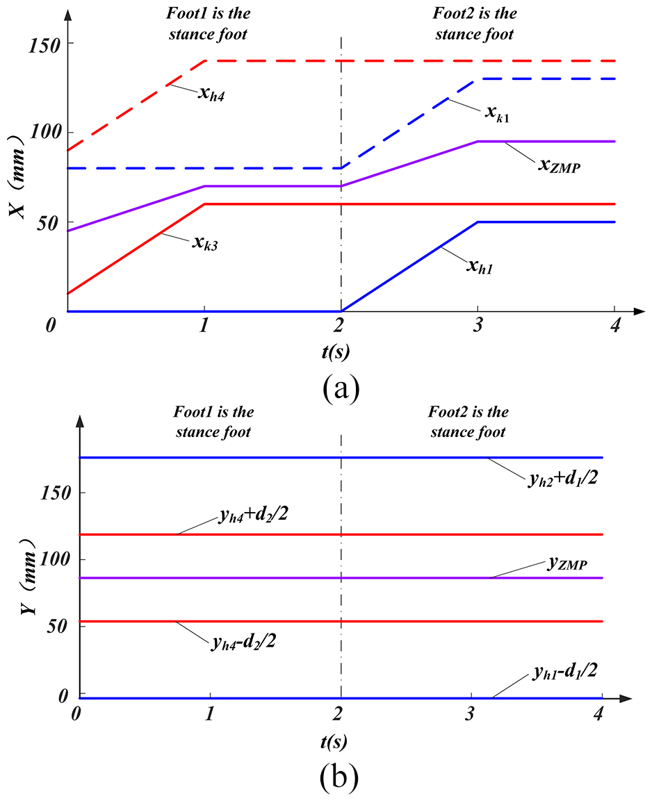
Figure 14 (a) Motion along the x-axis x_h1, x_h4, x_k1, x_k3, and x_ZMP trajectory graph. (b) Motion along the x-axis $y_{h\mathrm{1}}-d_{\mathrm{1}}/\mathrm{2}$, $y_{h\mathrm{2}}+d_{\mathrm{1}}/\mathrm{2}$, $y_{h\mathrm{4}}-d_{\mathrm{2}}/\mathrm{2}$, $y_{h\mathrm{4}}+d_{\mathrm{2}}/\mathrm{2}$, and y_ZMP trajectory graph.

As illustrated in Fig. 14, the ZMP consistently resides within the support range during the movement of the HFCM along the x axis, thereby satisfying the condition of static stability.

As the HFCM traverses the y axis, the trajectories of x_h1, x_h4, x_k1, x_k3, and x_ZMP are depicted in Fig. 15a, while the trajectories of y_h1, y_h2, $y_{h\mathrm{3}}-d_{\mathrm{2}}/\mathrm{2}$, $y_{h\mathrm{3}}+d_{\mathrm{2}}/\mathrm{2}$, and y_ZMP are illustrated in Fig. 15b.

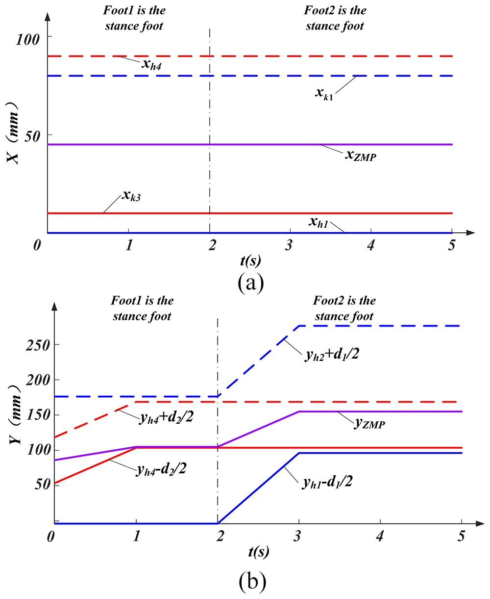
Figure 15 (a) Motion along the y-axis x_h1, x_h4, x_k1, x_k3, and x_ZMP trajectory graph. (b) Motion along the y-axis y_h1, y_h2, $y_{h\mathrm{3}}-d_{\mathrm{2}}/\mathrm{2}$, $y_{h\mathrm{3}}+d_{\mathrm{2}}/\mathrm{2}$, and y_ZMP trajectory graph.

As demonstrated in Fig. 15, during the movement of the HFCM along the y axis, x_ZMP remains within the support range at all times, while y_ZMP approaches the line $y_{h\mathrm{3}}-d_{\mathrm{2}}/\mathrm{2}$ at the 16 s mark. However, it remains above the line $y_{h\mathrm{3}}-d_{\mathrm{2}}/\mathrm{2}$, which remains within the support range. This fulfils the condition of static stability.

Consequently, the HFCM is capable of moving in a smooth and continuous straight line along both the x axis and y axis. Furthermore, by integrating the gaits of linear movement along the x axis and y axis, the HFCM is capable of achieving movement between any position on the plane

3.2 HFCM kinematic analysis

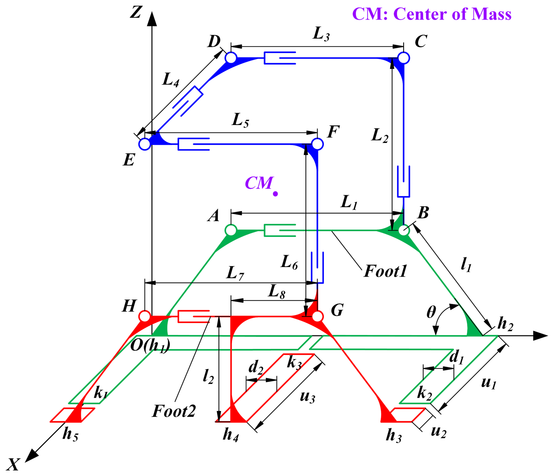
A simplified scheme of the HFCM is shown in Fig. 16. In the figure, points A, B, C, D, E, F, G, and H are the centre of mass of each connecting link. L_i (i=1, 2, 3, 4, 5, 6, 7) are the distances to the neighbouring centres of mass, respectively, and are the distances from the support structure in the middle of Foot2 to the G points. h_i (i=1, 2, 3, 4, 5) are the connection points between the support rods and the base plate in each support structure. k₁k₂ are the centres of the ends of the two base plates in Foot1, and k₃ is the centre point of the end of the middle base plate of Foot2. l₁ is the length of the support rods in the support mechanism on both sides in Foot1 and Foot2. l₂ is the length of the support bar in the Foot2 intermediate support mechanism. θ is the angle between the support bar and the base plate on both sides in Foot1 and Foot2. u₁ is the length of the bottom plate on both sides in Foot1. u₂ is the length of the bottom plate on both sides in Foot2. u₃ is the length of the middle base plate of Foot2. The width of the bottom plate on both sides in Foot1 and Foot2 is d₁. The width of the Foot2 intermediate base plate is d₂. Δl is the travelling distance of each moving joint. The time for each joint to complete Δl telescopic stroke is t₁. The centre of mass (CM) of the HFCM is located at the centre of the system. The CM coordinates are as follows:

$$\begin{array}{}\text{(6)}& \mathrm{CM}={\left[\begin{array}{ccc}{\mathrm{CM}}_x& {\mathrm{CM}}_y& {\mathrm{CM}}_z\end{array}\right]}^T.\end{array}$$

The objective of the positive kinematic analysis is to ascertain the coordinates of points h₃ and h₄ for stationary footholds and points h₁ and h₂ for stationary footholds during the linear travel of the HFCM along the x axis and y axis, utilizing the aforementioned parameters.

$$\begin{array}{}\text{(7)}& \begin{array}{rl}& A={\left[\begin{array}{ccc}{x}_{h\mathrm{1}}& y_{h\mathrm{1}}+I_{\mathrm{1}}& z_{h\mathrm{1}}+I_{\mathrm{2}}\end{array}\right]}^T\\ & B={\left[\begin{array}{ccc}{x}_{h\mathrm{1}}& y_{h\mathrm{1}}+I_{\mathrm{1}}+L_{\mathrm{1}}& z_{h\mathrm{1}}+I_{\mathrm{2}}\end{array}\right]}^T\\ & C={\left[\begin{array}{ccc}{x}_{h\mathrm{1}}& y_{h\mathrm{1}}+I_{\mathrm{1}}+L_{\mathrm{1}}& z_{h\mathrm{1}}+I_{\mathrm{2}}+L_{\mathrm{2}}\end{array}\right]}^T\\ & D={\left[\begin{array}{ccc}{x}_{h\mathrm{1}}& y_{h\mathrm{1}}+I_{\mathrm{1}}+L_{\mathrm{1}}-L_{\mathrm{3}}& z_{h\mathrm{1}}+I_{\mathrm{2}}+L_{\mathrm{2}}\end{array}\right]}^T\\ & E={\left[\begin{array}{ccc}{x}_{h\mathrm{1}}+L_{\mathrm{4}}& y_{h\mathrm{1}}+I_{\mathrm{1}}+L_{\mathrm{1}}-L_{\mathrm{3}}& z_{h\mathrm{1}}+I_{\mathrm{2}}+L_{\mathrm{2}}\end{array}\right]}^T\\ & F={\left[\begin{array}{ccc}{x}_{h\mathrm{1}}+L_{\mathrm{4}}& y_{h\mathrm{1}}+I_{\mathrm{1}}+L_{\mathrm{1}}-L_{\mathrm{3}}+L_{\mathrm{5}}& z_{h\mathrm{1}}+I_{\mathrm{2}}+L_{\mathrm{2}}\end{array}\right]}^T\\ & G={\left[\begin{array}{ccc}{x}_{h\mathrm{1}}+L_{\mathrm{4}}& y_{h\mathrm{1}}+I_{\mathrm{1}}+L_{\mathrm{1}}-L_{\mathrm{3}}+L_{\mathrm{5}}& z_{h\mathrm{1}}+I_{\mathrm{2}}+L_{\mathrm{2}}-L_{\mathrm{6}}\end{array}\right]}^T\\ & H={\left[\begin{array}{ccc}{x}_{h\mathrm{1}}+L_{\mathrm{4}}& y_{h\mathrm{1}}+I_{\mathrm{1}}+L_{\mathrm{1}}-L_{\mathrm{3}}+L_{\mathrm{5}}-L_{\mathrm{8}}& z_{h\mathrm{1}}+I_{\mathrm{2}}+L_{\mathrm{2}}-L_{\mathrm{6}}\end{array}\right]}^T\end{array}\end{array}$$

Here, I₁=l₁cos θ, and I₂=l₁sin θ.

Figure 16 Simplified scheme of HFCM.

Using the coordinates of the points of the curve, the coordinates of the turning point h_i (i=1, 2, 3, 4, 5) can be expressed as

$$\begin{array}{}\text{(8)}& \begin{array}{rl}& h_{\mathrm{1}}={\left[\begin{array}{ccc}{x}_{h\mathrm{1}}& y_{h\mathrm{1}}& z_{h\mathrm{1}}\end{array}\right]}^T,\\ & h_{\mathrm{2}}={\left[\begin{array}{ccc}{x}_B& y_B+I_{\mathrm{1}}& z_B-I_{\mathrm{2}}\end{array}\right]}^T,\\ & h_{\mathrm{3}}={\left[\begin{array}{ccc}{x}_G& y_G+I_{\mathrm{1}}& z_G-I_{\mathrm{2}}\end{array}\right]}^T,\\ & h_{\mathrm{4}}={\left[\begin{array}{ccc}{x}_G& y_G+L_{\mathrm{8}}& z_G-l_{\mathrm{2}}\end{array}\right]}^T,\\ & h_{\mathrm{5}}={\left[\begin{array}{ccc}{x}_H& y_H-I_{\mathrm{1}}& z_H-I_{\mathrm{2}}\end{array}\right]}^T.\end{array}\end{array}$$

When it is a station, the coordinates of the points in the curve in the world coordinate system can be obtained from the point h₄.

$$\begin{array}{}\text{(9)}& \begin{array}{rl}& A={\left[\begin{array}{ccc}{x}_{h\mathrm{5}}-L_{\mathrm{4}}& y_{h\mathrm{5}}+I_{\mathrm{1}}+L_{\mathrm{7}}-L_{\mathrm{5}}+L_{\mathrm{3}}-L_{\mathrm{1}}& z_{h\mathrm{5}}+I_{\mathrm{2}}+L_{\mathrm{6}}-L_{\mathrm{2}}\end{array}\right]}^T\\ & B={\left[\begin{array}{ccc}{x}_{h\mathrm{5}}-L_{\mathrm{4}}& y_{h\mathrm{5}}+I_{\mathrm{1}}+L_{\mathrm{7}}-L_{\mathrm{5}}+L_{\mathrm{3}}& z_{h\mathrm{5}}+I_{\mathrm{2}}+L_{\mathrm{6}}-L_{\mathrm{2}}\end{array}\right]}^T\\ & C={\left[\begin{array}{ccc}{x}_{h\mathrm{5}}-L_{\mathrm{4}}& y_{h\mathrm{5}}+I_{\mathrm{1}}+L_{\mathrm{7}}-L_{\mathrm{5}}+L_{\mathrm{3}}& z_{h\mathrm{5}}+I_{\mathrm{2}}+L_{\mathrm{6}}\end{array}\right]}^T\\ & D={\left[\begin{array}{ccc}{x}_{h\mathrm{5}}-L_{\mathrm{4}}& y_{h\mathrm{5}}+I_{\mathrm{1}}+L_{\mathrm{7}}-L_{\mathrm{5}}& z_{h\mathrm{5}}+I_{\mathrm{2}}+L_{\mathrm{6}}\end{array}\right]}^T\\ & E={\left[\begin{array}{ccc}{x}_{h\mathrm{5}}& y_{h\mathrm{5}}+I_{\mathrm{1}}+L_{\mathrm{7}}-L_{\mathrm{5}}& z_{h\mathrm{5}}+I_{\mathrm{2}}+L_{\mathrm{6}}\end{array}\right]}^T\\ & F={\left[\begin{array}{ccc}{x}_{h\mathrm{5}}& y_{h\mathrm{5}}+I_{\mathrm{1}}+L_{\mathrm{7}}& z_{h\mathrm{5}}+I_{\mathrm{2}}+L_{\mathrm{6}}\end{array}\right]}^T\\ & G={\left[\begin{array}{ccc}{x}_{h\mathrm{5}}& y_{h\mathrm{5}}+I_{\mathrm{1}}+L_{\mathrm{7}}& z_{h\mathrm{5}}+I_{\mathrm{2}}\end{array}\right]}^T\\ & H={\left[\begin{array}{ccc}{x}_{h\mathrm{5}}& y_{h\mathrm{5}}+I_{\mathrm{1}}& z_{h\mathrm{4}}+I_{\mathrm{2}}\end{array}\right]}^T\end{array}\end{array}$$

Using the coordinates of the points of the middle curve, the coordinates of the turning point $h_i\left(i=\mathrm{1},\mathrm{2},\mathrm{3},\mathrm{4},\mathrm{5}\right)$ can be expressed as

$$\begin{array}{}\text{(10)}& \begin{array}{rl}& h_{\mathrm{1}}={\left[\begin{array}{ccc}{x}_A& y_A-I_{\mathrm{1}}& z_A-I_{\mathrm{2}}\end{array}\right]}^T,\\ & h_{\mathrm{2}}={\left[\begin{array}{ccc}{x}_B& y_B+I_{\mathrm{1}}& z_B-I_{\mathrm{2}}\end{array}\right]}^T,\\ & h_{\mathrm{3}}={\left[\begin{array}{ccc}{x}_G& y_G+I_{\mathrm{1}}& z_G-I_{\mathrm{2}}\end{array}\right]}^T,\\ & h_{\mathrm{4}}={\left[\begin{array}{ccc}{x}_G& y_G-L_{\mathrm{8}}& z_G-I_{\mathrm{2}}\end{array}\right]}^T,\\ & h_{\mathrm{5}}={\left[\begin{array}{ccc}{x}_{h\mathrm{5}}& y_{h\mathrm{5}}& z_{h\mathrm{5}}\end{array}\right]}^T.\end{array}\end{array}$$

Using the coordinates of h_i (i=1, 2, 3, 4, 5), the coordinates of k_i (i=1, 2, 3) can be expressed as

$$\begin{array}{}\text{(11)}& \begin{array}{rl}& k_{\mathrm{1}}={\left[\begin{array}{ccc}{x}_{h\mathrm{1}}+u_{\mathrm{1}}& y_{h\mathrm{1}}& z_{h\mathrm{1}}\end{array}\right]}^T,\\ & k_{\mathrm{2}}={\left[\begin{array}{ccc}{x}_{h\mathrm{2}}+u_{\mathrm{1}}& y_{h\mathrm{2}}& z_{h\mathrm{2}}\end{array}\right]}^T,\\ & k_{\mathrm{3}}={\left[\begin{array}{ccc}{x}_{h\mathrm{4}}-u_{\mathrm{3}}& y_{h\mathrm{4}}& z_{h\mathrm{4}}\end{array}\right]}^T.\end{array}\end{array}$$

In accordance with the established principles of motion (a) to (e) as illustrated in Fig. 4, the equation for the variation of L_i (i=1, 2, 3, 4, 5, 6, 7) with time in the continuous motion of the HFCM along the x axis is as follows:

$$\begin{array}{}\text{(12)}& \begin{array}{rl}& \left\{\begin{array}{l}{L}_{\mathrm{1}}=L_{AB}\\ L_{\mathrm{2}}=L_{BC}+\left(t-T_{\mathrm{1}}-T_{\mathrm{2}}+\mathrm{2}{T}_{\mathrm{3}}\right)v\\ L_{\mathrm{3}}=L_{CD}\\ L_{\mathrm{4}}=L_{DE}+\left(t-T_{\mathrm{1}}-T_{\mathrm{2}}+T_{\mathrm{3}}\right)v\\ L_{\mathrm{5}}=L_{EF}\\ L_{\mathrm{6}}=L_{FG}+\left(T_{\mathrm{1}}-T_{\mathrm{2}}\right)v\\ L_{\mathrm{7}}=L_{GH}\\ T_i=\frac{\left|t-i{t}_{\mathrm{1}}\right|+\left(t-i{t}_{\mathrm{1}}\right)}{\mathrm{2}}\left(i=\mathrm{1},\mathrm{2},\mathrm{3}\mathrm{\dots }\right),v=\frac{\mathrm{\Delta }l}{t_{\mathrm{1}}}\end{array}\right.,\\ & t\in \left[\mathrm{0},\mathrm{4}{t}_{\mathrm{1}}\right]\end{array}\end{array}$$

where L_AB, L_BC, L_CD, L_DE, L_FG, and L_GH are the distances of each point in the initial state. From the simplified scheme of the mechanism and the motion principle (Fig. 4a–e), it can be seen that when the HFCM moves continuously along the x axis, Foot1 is a stationary footing when $t\in [\mathrm{0},\mathrm{2}{t}_{\mathrm{1}}]$, which corresponds to Eqs. (7) and (8):

$$\begin{array}{}\text{(13)}& h_{\mathrm{1}}={\left[\begin{array}{ccc}{x}_{h\mathrm{1}}& y_{h\mathrm{1}}& z_{h\mathrm{1}}\end{array}\right]}^T={\left[\begin{array}{ccc}\mathrm{0}& \mathrm{0}& \mathrm{0}\end{array}\right]}^T.\end{array}$$

When $t\in (\mathrm{2}{t}_{\mathrm{1}},\mathrm{4}{t}_{\mathrm{1}}]$, Foot2 is station-based, corresponding to Eqs. (8) and (9):

$$\begin{array}{}\text{(14)}& h_{\mathrm{5}}={\left[\begin{array}{ccc}{x}_{h\mathrm{5}}& y_{h\mathrm{5}}& z_{h\mathrm{5}}\end{array}\right]}^T={\left[\begin{array}{ccc}{L}_{DE}+\mathrm{\Delta }l& \mathrm{0}& \mathrm{0}\end{array}\right]}^T.\end{array}$$

From Eqs. (7)–(10), (12), and (13), the trajectories of the points in the continuous motion of the HFCM along the x axis in space and the displacements in the direction of the z axis are calculated. These are calculated using Eqs. (7), (8), (12), and (13) when $t\in [\mathrm{0},\mathrm{2}{t}_{\mathrm{1}}]$. In the event of $t\in (\mathrm{2}{t}_{\mathrm{1}},\mathrm{4}{t}_{\mathrm{1}}]$, the calculation and plotting of Eqs. (9), (10), (12), and (14) as images is to be conducted using MATLAB. Figure 17a demonstrates the trajectory of h_i when the HFCM is moving along the x axis, and Fig. 17b illustrates the displacement of h_i in the direction of the z axis when the HFCM is moving along the x axis.

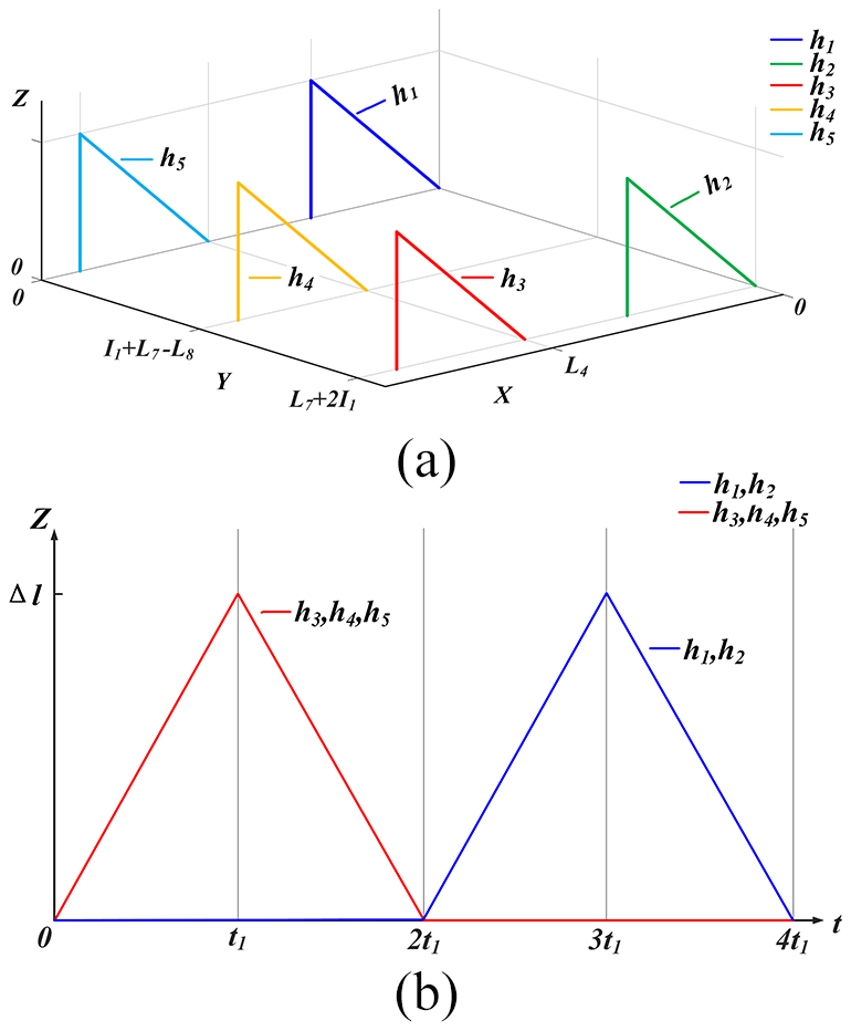
Figure 17 (a) Trajectory of g during motion along the x axis. (b) Displacement of j in the direction of the z axis during motion along the x axis.

According to motion principles (a)–(f) shown in Fig. 5, the equation of variation of L_i with time in the continuous motion of the HFCM along the y axis is

$$\begin{array}{}\text{(15)}& \begin{array}{rl}& \left\{\begin{array}{l}{L}_{\mathrm{1}}=L_{AB}\\ L_{\mathrm{2}}=L_{BC}+\left(t-T_{\mathrm{1}}-T_{\mathrm{2}}+\mathrm{2}{T}_{\mathrm{3}}-T_{\mathrm{4}}\right)v\\ L_{\mathrm{3}}=L_{CD}+\left(T_{\mathrm{2}}-T_{\mathrm{3}}\right)v\\ L_{\mathrm{4}}=L_{DE}\\ L_{\mathrm{5}}=L_{EF}+\left(t-T_{\mathrm{1}}-T_{\mathrm{2}}+T_{\mathrm{3}}\right)v\\ L_{\mathrm{6}}=L_{FG}+\left(T_{\mathrm{1}}-T_{\mathrm{2}}-T_{\mathrm{4}}\right)v\\ L_{\mathrm{7}}=L_{GH}\end{array}\right..\\ & t\in \left[\mathrm{0},\mathrm{5}{t}_{\mathrm{1}}\right]\end{array}\end{array}$$

In a similar manner, an examination of the motion schematic (see Fig. 5a–f) reveals that when the HFCM moves continuously along the y axis, Foot1 is the stationary footing when $t\in [\mathrm{0},\mathrm{2}{t}_{\mathrm{1}}]$, which corresponds to Eqs. (7) and (8):

$$\begin{array}{}\text{(16)}& h_{\mathrm{1}}={\left[\begin{array}{ccc}{x}_{h\mathrm{1}}& y_{h\mathrm{1}}& z_{h\mathrm{1}}\end{array}\right]}^T={\left[\begin{array}{ccc}\mathrm{0}& \mathrm{0}& \mathrm{0}\end{array}\right]}^T.\end{array}$$

When $t\in [\mathrm{2}{t}_{\mathrm{1}},\mathrm{5}{t}_{\mathrm{1}}]$, Foot2 is station-based, corresponding to Eqs. (9) and (10):

$$\begin{array}{}\text{(17)}& h_{\mathrm{5}}={\left[\begin{array}{ccc}{x}_{h\mathrm{5}}& y_{h\mathrm{5}}& z_{h\mathrm{5}}\end{array}\right]}^T={\left[\begin{array}{ccc}{L}_{DE}& \mathrm{\Delta }l& \mathrm{0}\end{array}\right]}^T.\end{array}$$

From Eqs. (7)–(10) and (15)–(17), the trajectory of the point h_i in space and the displacement in the direction of the z axis are calculated for the continuous motion of the HFCM along the y axis. When $t\in [\mathrm{0},\mathrm{2}{t}_{\mathrm{1}}]$, Eqs. (7), (8), (15), and (16) are used, and when $t\in [\mathrm{2}{t}_{\mathrm{1}},\mathrm{5}{t}_{\mathrm{1}}]$, Eqs. (9), (10), (15), and (17) are used, and the image is plotted. Figure 18a shows the trajectory diagram of h_i when the HFCM moves along the y axis, and Fig. 18b shows the displacement of h_i in the z-axis direction when the HFCM moves along the x axis.

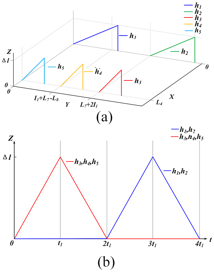
Figure 18 (a) Trajectory of h_i when moving along the y axis. (b) Displacement of h_i in the direction of the z axis during motion along the y axis.

3.3 Analysis of HFCM rotational kinematics

It is evident that HFCM is equipped with multiple base plate mechanisms in its two feet. The substantial contact area of these base plates with the ground can generate friction, which is introduced into the motion of HFCM. The rotating walking gait of HFCM is designed, and the principle of walking gait is explained as follows.

Figure 19 (a) Sketch of initial attitude of rotation. (b) Sketch of completed rotation.

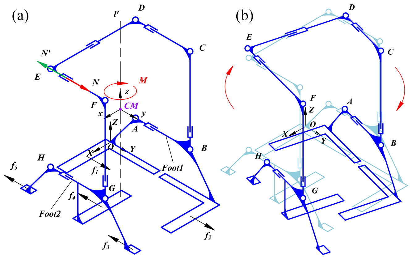
As demonstrated in Fig. 19, the curve undergoes a transformation to the configuration depicted in Fig. 19a through the deformation process illustrated in Fig. 4a and b. Subsequently, the mobile mechanism situated between EF undergoes an extension, resulting in an expansion of EF. During the extension of the mobile mechanism between EF, this results in the application of a driving force of magnitude N to the FGH portion of the HFCM, causing the FGH portion to move forward. The reaction force, N^′, is generated by this driving force and acts on the ABCDE portion of the HFCM, leading to its backward movement. The reaction force, N^′, is generated by this driving force and acts on the ABCDE portion of the HFCM, causing the portion to move backward. Consequently, Foot1 and Foot2 will move in opposite directions under the action of the driving force N. The base plates in contact with the ground in Foot1 and Foot2 will generate a sliding friction force, f_i (i=1, 2, 3, 4, 5), at this movement.

It is evident that points f₁ and f₂ are oriented in a direction that is contrary to that of points f₃, f₄, and f₅. Furthermore, it is notable that these points do not intersect with the centre of mass of the machine. This configuration results in the generation of a moment M, which is exerted under the influence of f_i. The consequence of this interaction is the rotation of the HFCM in a specific axis, designated as axis l^′. The direction of rotation along this axis is defined as clockwise.

The establishment of CM-xyz, set l^′, is to be executed over the centre of mass of the HFCM, with the subsequent perpendicularity to the XWY plane being a requisite element of this process. The initial coordinates and attitude of the CM-xyz coordinate system in the O-xyz coordinate system are represented as follows:

$$\begin{array}{}\text{(18)}& {}_{\mathrm{CM}}^{O}P=\left[\begin{array}{cccc}{r}_{\mathrm{CM}xx}& r_{\mathrm{CM}yx}& r_{\mathrm{CM}zx}& p_{\mathrm{CM}x}\\ r_{\mathrm{CM}xy}& r_{\mathrm{CM}yy}& r_{\mathrm{CM}zy}& p_{\mathrm{CM}y}\\ r_{\mathrm{CM}xz}& r_{\mathrm{CM}yz}& r_{\mathrm{CM}zz}& p_{\mathrm{CM}z}\\ \mathrm{0}& \mathrm{0}& \mathrm{0}& \mathrm{1}\end{array}\right].\end{array}$$

The initial χ² coordinates of h_i in the CM-xy coordinate system are expressed as

$$\begin{array}{}\text{(19)}& {}_{h_i}^{\mathrm{CM}}P={\left[\begin{array}{cccc}{x}_i& y_i& \mathrm{0}& \mathrm{1}\end{array}\right]}^T.\end{array}$$

In this particular gait, the motion of CM-xy is characterized as a translational transformation, whereas h_i is designated as a rotational transformation with respect to CM-xy. Consequently, the transformation of h_i is identified as a composite transformation. The transformation matrix during rotation is expressed as follows:

$$\begin{array}{}\text{(20)}& \begin{array}{rl}& T\left({}_{\mathrm{CM}}^{O}P\right)={\left[\begin{array}{cccc}\mathrm{1}& \mathrm{0}& \mathrm{0}& \mathrm{\Delta }x\\ \mathrm{0}& \mathrm{1}& \mathrm{0}& \mathrm{\Delta }y\\ \mathrm{0}& \mathrm{0}& \mathrm{1}& \mathrm{\Delta }z\\ \mathrm{0}& \mathrm{0}& \mathrm{0}& \mathrm{1}\end{array}\right]}^T,\\ & {}_{h_i}^{\mathrm{CM}}R\left(Z,\mathit{\alpha }\right)={\left[\begin{array}{cccc}c\mathit{\alpha }& -s\mathit{\alpha }& \mathrm{0}& \mathrm{0}\\ s\mathit{\alpha }& c\mathit{\alpha }& \mathrm{0}& \mathrm{0}\\ \mathrm{0}& \mathrm{0}& \mathrm{1}& \mathrm{0}\\ \mathrm{0}& \mathrm{0}& \mathrm{0}& \mathrm{1}\end{array}\right]}^T,\end{array}\end{array}$$

where α is the angle of rotation.

Therefore, the coordinates of h_i after the rotational transformation with respect to the O-xyz coordinate system are

$$\begin{array}{}\text{(21)}& {}_{h_i}^{O}P=T{\left({}_{\mathrm{CM}}^{O}P\right)}_{\mathrm{CM}}^O{P}_{h_i}^{\mathrm{CM}}R{\left(Z,\mathit{\alpha }\right)}_{h_i}^{\mathrm{CM}}P.\end{array}$$

When the EF is fully extended, the position of the HFCM undergoes a transformation as depicted in Fig. 19b. Through the repetition of this process, the HFCM can be made to rotate continuously clockwise.

A similar effect can be achieved by expanding the DC part in the attitude of Fig. 19a, thereby inducing an anticlockwise rotation of the HFCM.

Figure 20 Establishment of the HSCM coordinate system.

3.4 HSCM stability analysis

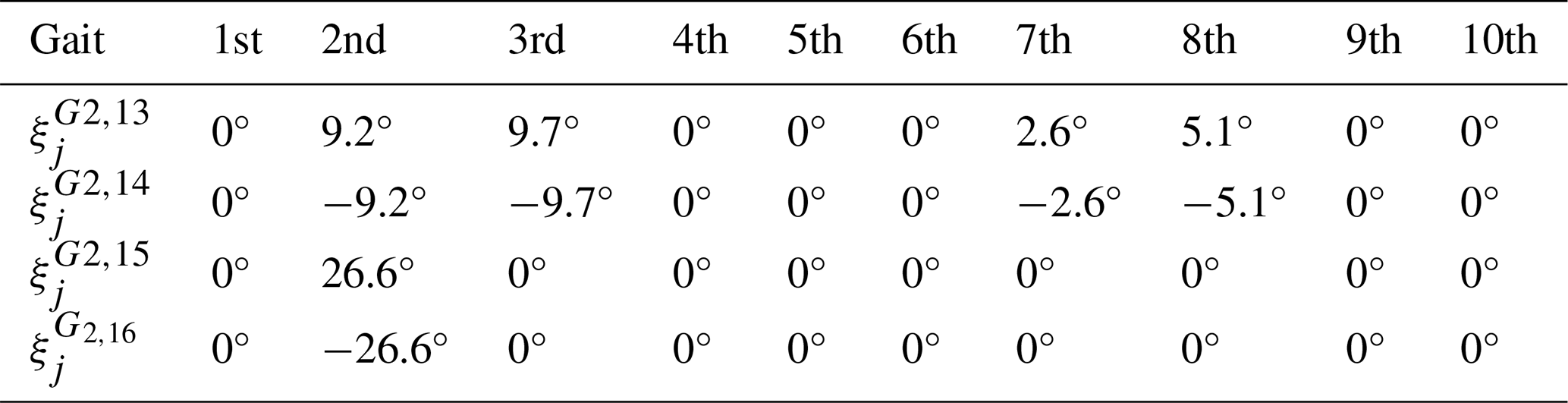
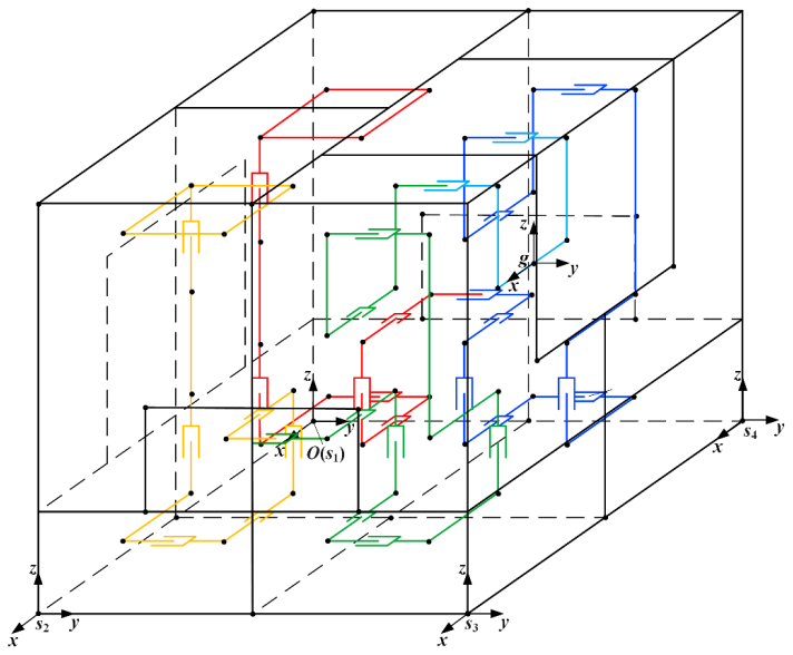
It is evident that gaits G_2,1–G_2,18 in G_2,1–G_2,17 and G_2,18 are executed in an upright position. It is discernible that the equivalent support range is considerably more extensive than that of the G_2,13–G_2,16 mechanism in a tilted state. Consequently, it is reasonable to conclude that the G_2,13–G_2,16 gait is more prone to tilting than the other gaits during operation. Therefore, the primary objective of the stability analysis of the HSCM is to ascertain the stability of G_2,13–G_2,16. As demonstrated in Figs. 6b and 20, the origin O of the fixed coordinate system O−XYZ is consistently located on the ground at points e₂, e₇, e₁₂, and e₁₃ and at the midpoint of the straight line segment A₃₂A₃₃. Initially, this coincides with the bottom vertex e₁₃ of the robot. The x axis corresponds to e₁₃e₂, the y axis corresponds to e₁₃e₁₂, and the z axis corresponds to e₁₃e₃₀. The origin of the coordinate system S_i-xyz is always located at e₂, e₇, e₁₂, and e₁₃, the origin of g-xyz is always located at the centre of the line segment A₃₂A₃₃, and the node connector at the corresponding position is N₁₆. In the initial state, the x, y, and z axes of all dynamic coordinate systems are parallel to the x, y, and z axes of the fixed coordinate system, respectively. The centre of mass (CM2) of the HSCM in the coordinate system g-xyz can be solved by the centre of mass coordinates as follows:

$$\begin{array}{}\text{(22)}& x_{{\mathrm{CM}}_{\mathrm{2}}}^g={\displaystyle \frac{\sum _{i=\mathrm{1}}^n{M}_i{x}_{{\mathrm{CM}}_{i^{\prime }}}^g}{\sum _{i=\mathrm{1}}^n{M}_i{y}_{{\mathrm{CM}}_{\mathrm{2}}}^g}}={\displaystyle \frac{\sum _{i=\mathrm{1}}^n{M}_i{y}_{{\mathrm{CM}}_{i^{\prime }}}^g}{\sum _{i=\mathrm{1}}^n{M}_i{z}_{{\mathrm{CM}}_{\mathrm{2}}}^g}}={\displaystyle \frac{\sum _{i=\mathrm{1}}^n{M}_i{z}_{{\mathrm{CM}}_{i^{\prime }}}^g}{\sum _{i=\mathrm{1}}^n{M}_i}},\end{array}$$

where $x_{{\mathrm{CM}}_{\mathrm{2}}}^g$, $y_{{\mathrm{CM}}_{\mathrm{2}}}^g$, $z_{{\mathrm{CM}}_{\mathrm{2}}}^g$ is the centre of mass coordinate of the mechanism in the coordinate system g-xyz. n is the number of HSCM node connection blocks. $x_{{\mathrm{CM}}_i}^g$, $y_{{\mathrm{CM}}_i}^g$, $z_{{\mathrm{CM}}_i}^g$ denotes the centre of mass coordinates of the ith node connector in the coordinate system g-xyz. Under the coordinate system O-xyz, the initial position and attitude of the coordinate system S_i-xyz are represented as follows:

$$\begin{array}{}\text{(23)}& \begin{array}{rl}& {}_{S_i}^{O}R=\left[\begin{array}{ccc}{r}_{s_i,xx}& r_{s_i,yx}& r_{s_i,zx}\\ r_{s_i,xy}& r_{s_i,yy}& r_{s_i,zy}\\ r_{s_i,xz}& r_{s_i,yz}& r_{s_i,zz}\end{array}\right],\\ & {}_{S_i}^{O}P=\left[\begin{array}{l}{p}_{s_i,x}\\ p_{s_i,y}\\ p_{s_i,z}\end{array}\right].\end{array}\end{array}$$

Under the coordinate system S_i-xyz, the initial position and attitude of the coordinate system g-xyz are represented as follows:

$$\begin{array}{}\text{(24)}& \begin{array}{rl}& {}_g^{S_i}P={\left[\begin{array}{ccc}{x}_i& y_i& z_i\end{array}\right]}^T,\\ & {}_g^{S_i}R=\left[\begin{array}{ccc}{r}_{gxx}& r_{gyx}& r_{gzx}\\ r_{gxy}& r_{gyy}& r_{gzy}\\ r_{gxz}& r_{gyz}& r_{gzz}\end{array}\right].\end{array}\end{array}$$

In the coordinate system g-xyz, the initial coordinates of vertex A_i are expressed as follows:

$$\begin{array}{}\text{(25)}& {}_{A_i}^{g}P={\left[\begin{array}{ccc}{x}_i& y_i& z_i\end{array}\right]}^T.\end{array}$$

When certain telescopic rods are extended or shortened, the relative displacement of point A_i in the coordinate system g-xyz is expressed as follows:

$$\begin{array}{}\text{(26)}& \mathrm{\Delta }{A}_i={\left[\begin{array}{ccc}\mathrm{\Delta }{x}_i& \mathrm{\Delta }{y}_i& \mathrm{\Delta }{z}_i\end{array}\right]}^T.\end{array}$$

The initial coordinates of vertex e_i in the g-xyz coordinate system are expressed as follows:

$$\begin{array}{}\text{(27)}& {}_{e_i}^{g}P={\left[\begin{array}{ccc}{x}_i& y_i& z_i\end{array}\right]}^T.\end{array}$$

When certain telescopic rods are extended or shortened, the relative displacement of point e_i in the coordinate system g-xyz is expressed as follows:

$$\begin{array}{}\text{(28)}& \mathrm{\Delta }{e}_i={\left[\begin{array}{ccc}\mathrm{\Delta }{x}_i& \mathrm{\Delta }{y}_i& \mathrm{\Delta }{z}_i\end{array}\right]}^T.\end{array}$$

From the gait planning, it can be concluded that when the robot performs G_2,13–G_2,18 gaits, the coordinate system S_i-xyz will do only translational motion in the coordinate system O-xyz, while the coordinate system g-xyz will do composite motion in the coordinate system S_i-xyz. Therefore, the translation matrix of the coordinate system S_i-xyz in the coordinate system O-xyz at the jth step can be expressed as

$$\begin{array}{}\text{(29)}& \begin{array}{rl}& {}_g^{s_i}{P}_{j+\mathrm{1}}=T_j{(}_g^{s_i}P){+}_g^{s_i}{P}_j,\\ & {}_g^{s_i}{R}_{j+\mathrm{1}}=R{\left({\mathit{\psi }}_{j+\mathrm{1}}^{G_{\mathrm{2},i}},{\mathit{\xi }}_{j+\mathrm{1}}^{G_{\mathrm{2},i}}\right)}_g^{s_i}{R}_j.\end{array}\end{array}$$

The translation matrix of the coordinate system g-xyz in the coordinate system S_i-xyz at step j can be expressed as

$$\begin{array}{}\text{(30)}& T_j\left({}_g^{s_i}P\right)={\left[\begin{array}{ccc}\mathrm{\Delta }\mathrm{d}x& \mathrm{\Delta }\mathrm{d}y& \mathrm{\Delta }\mathrm{d}z\end{array}\right]}^T.\end{array}$$

After its own deformation, the representation of the position of the coordinate system S_i-xyz in step j+1 is updated under the coordinate system O-xyz as

$$\begin{array}{}\text{(31)}& {}_g^{s_i}{P}_{j+\mathrm{1}}=T_j\left({}_{s_i}^{O}P\right){+}_{s_i}^O{P}_j,\text{(32)}& {}_{s_i}^O{R}_{j+\mathrm{1}}{=}_{s_i}^O{R}_j.\end{array}$$

After the first step, the position of the coordinate system g-xyz in the coordinate system S_i-xyz is calculated as follows:

$$\begin{array}{}\text{(33)}& {}_g^{s_i}{P}_{j+\mathrm{1}}=T_j\left({}_g^{s_i}P\right){+}_g^{s_i}{P}_j,\text{(34)}& {}_g^{s_i}{R}_{j+\mathrm{1}}=R{\left({\mathit{\psi }}_{j+\mathrm{1}}^{G_{\mathrm{2},i}},{\mathit{\xi }}_{j+\mathrm{1}}^{G_{\mathrm{2},i}}\right)}_g^{s_i}{R}_j.\end{array}$$

$R\left({\mathit{\psi }}_{j+\mathrm{1}}^{G_{\mathrm{2},i}}{\mathit{\xi }}_{j+\mathrm{1}}^{G_{\mathrm{2},i}}\right)$ is the rotation matrix, ${\mathit{\psi }}_j^{G_{\mathrm{2},i}}$ is the rotation axis of G_2,i at step j, and ${\mathit{\xi }}_j^{G_{\mathrm{2},i}}$ is the rotation angle of G_2,i at step j. From the gait planning, we can derive the rotation axis of step j corresponding to gait G₁₃–G₁₆ when the mechanism performs the G₁₃–G₁₆ gait. The rotation matrix for rotation around the x axis and y axis of the coordinate system S_i-xyz is

$$\begin{array}{}\text{(35)}& \begin{array}{rl}& R\left(x_{s_i}{\mathit{\xi }}_j^{G_{\mathrm{2},i}}\right)=\left[\begin{array}{cccc}\mathrm{1}& \mathrm{0}& \mathrm{0}& \mathrm{0}\\ \mathrm{0}& c{\mathit{\xi }}_j^{G_{\mathrm{2},i}}& -s{\mathit{\xi }}_j^{G_{\mathrm{2},i}}& \mathrm{0}\\ \mathrm{0}& s{\mathit{\xi }}_j^{G_{\mathrm{2},i}}& c{\mathit{\xi }}_j^{G_{\mathrm{2},i}}& \mathrm{0}\\ \mathrm{0}& \mathrm{0}& \mathrm{0}& \mathrm{1}\end{array}\right],\\ & R\left(y_{s_i}{\mathit{\xi }}_j^{G_{\mathrm{2},i}}\right)=\left[\begin{array}{cccc}c{\mathit{\xi }}_j^{G_{\mathrm{2},i}}& \mathrm{0}& s{\mathit{\xi }}_j^{G_{\mathrm{2},i}}& \mathrm{0}\\ \mathrm{0}& \mathrm{1}& \mathrm{0}& \mathrm{0}\\ -s{\mathit{\xi }}_j^{G_{\mathrm{2},i}}& \mathrm{0}& c{\mathit{\xi }}_j^{G_{\mathrm{2},i}}& \mathrm{0}\\ \mathrm{0}& \mathrm{0}& \mathrm{0}& \mathrm{1}\end{array}\right].\end{array}\end{array}$$

The coordinates of points A_i and e_i of the organization at step j+1 under the coordinate system O-xyz are computed as

$$\begin{array}{}\text{(36)}& {}_{A_i}^O{P}_j{=}_{s_i}^O{P}_{j+\mathrm{1}}{+}_{s_i}^{O}R\left({}_g^{S_i}{P}_{j+\mathrm{1}}{+}_g^{s_i}{R}_{j+\mathrm{1}}\left(P_{A_i}^{g}P+\mathrm{\Delta }{A}_i\right)\right),\text{(37)}& {}_{e_i}^O{P}_{j+\mathrm{1}}{=}_{s_i}^O{P}_{j+\mathrm{1}}{+}_{s_i}^{O}R\left({}_g^{S_i}{P}_{j+\mathrm{1}}{+}_g^{s_i}{R}_{j+\mathrm{1}}\left(P_{e_i}^g\mathrm{P}+\mathrm{\Delta }{e}_i\right)\right).\end{array}$$

From the obtained ${}_{A_i}^O{P}_j$, we can determine the coordinates of CM₂ at step j under the coordinate system O-xyz. From the obtained ${}_{e_i}^O{P}_j$, we can determine the support polygon of the robot in the state at step j under the coordinate system O-xyz.

Table 5 The parameters of M_i.

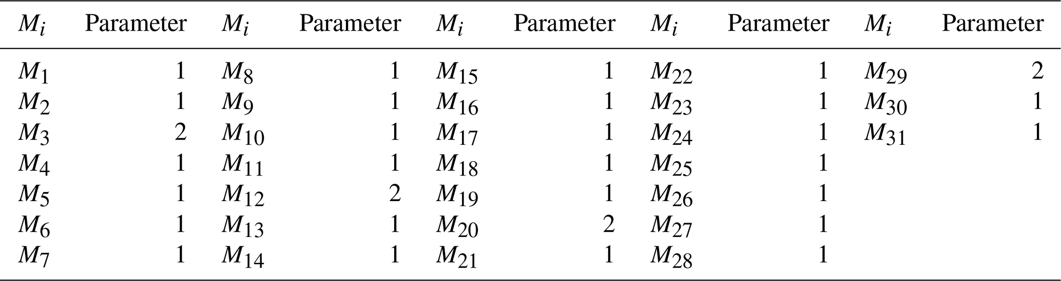
Based on the above analysis, a set of M_i parameters consistent with G_2,1–G_2,18 is derived, as shown in Table 5.

4 Simulation analysis

4.1 HFCM gait simulation

In the simulation, the parameters were configured as follows: the gravitational acceleration was set to 9.8 m s⁻², the static friction coefficient was 0.8, the dynamic friction coefficient was 0.7, and the material was specified as polylactic acid (PLA).

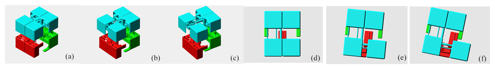
Figure 21 Rotational gait. (a) Gait 1, (b) gait 2, (c) gait 3, (d) gait 1 top view, (e) gait 2 top view, and (f) gait 3 top view.

The rotational simulation of the HFCM is shown in Fig. 21. The change in angular velocity of point A during the rotation with respect to the coordinates of CM is shown in Fig. 22. The angular velocity increases steadily and then decreases steadily, and CM_x and CM_y have only small changes in the overall motion, which is mainly caused by the deformation of the HFCM. For CM_z, no change occurs. During each cycle (6.3 s), a rotation angle of 14.2° was achieved. The average rotational speed was measured to be 2.25° s⁻¹ in the clockwise direction and 2.3° s⁻¹ in the anticlockwise direction. This indicates that the HFCM can rotate stably.

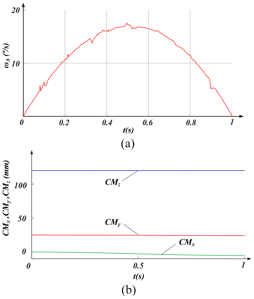
Figure 22 (a) Angular velocity of point A during rotation. (b) CM coordinate change during rotation.

4.2 HFCM step-up gait simulation

It is evident that the HFCM will be affected by gravity, which will likely result in its descent when the process of ascending the stairs reaches the point of lifting Foot1, as depicted in Fig. 23b. This occurrence renders the stair-climbing process impractical. To address this issue, the distribution of mass must be optimized to ensure the forward movement of the centre of gravity. Subsequently, the HFCM can elevate Foot1 in a stable manner, thereby completing the stair-climbing operation. The simulation depicted in Fig. 23 validates the feasibility of the proposed gait. Upon reaching Fig. 23e, it can be deduced that the HFCM has successfully ascended the stairs.

Figure 23 Step-up gait simulation. (a) t = 0 s. (b) t = 6 s. (c) t = 10.2 s. (d) t = 14.4 s. (e) t = 18.6 s. (f) t = 22.6 s.

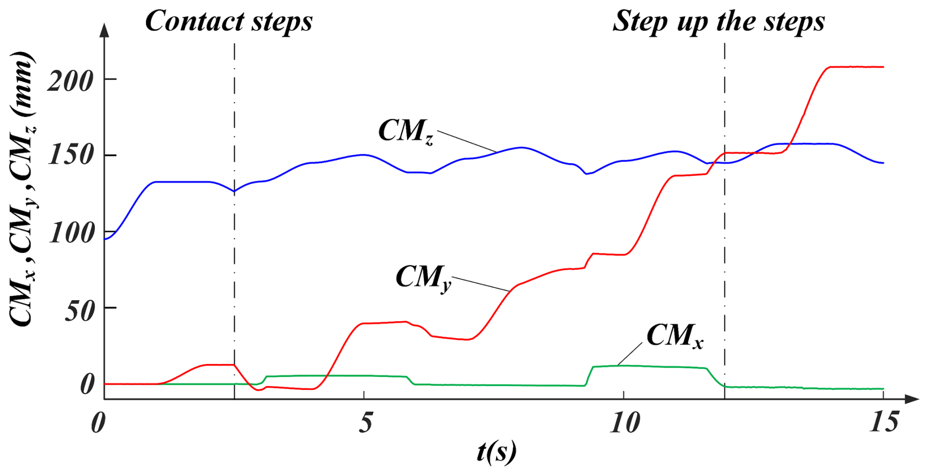
The coordinate change of CM over time during the simulation is shown in Fig. 24, which shows that the range of variation of CM_x during the motion is small and produces only a small change throughout the completion of the step-up gait. CM_y is the forward direction of the HFCM going up the step; after contacting the step, it increases gradually with the operation of the HFCM. The change in CM_z is related to the change in the HFCM's own shape and the height of the step. The change in the HFCM has a certain regularity, so the change in CM_z after contacting the step also has a certain regularity, and the change in CM_z after contacting the step has always been in a small range. According to the simulation results, the maximum step height achieved by the mechanism was 25 mm. This shows that the HFCM can stably complete the step-up operation.

Figure 24 CM coordinate changes during step ups.

4.3 HSCM simulation

4.3.1 HSCM plane shift simulation

The simulation process of G_2,1–G_2,4 completes one cycle, as shown in Figs. 25–28, respectively, and then repeats the cycle for five cycles, and the value of the centre of mass of N₁₆ on the coordinate axis changes as shown in Fig. 29. From Figs. 25–28, it can be concluded that when moving along the x axis, the x-axis coordinates change smoothly and regularly, and there is no obvious change in the y-axis coordinates; when moving along the y axis, the y-axis coordinates change smoothly and regularly, and there is no obvious change in the x-axis coordinates, which indicates that the HSCM can move along the x axis and y axis smoothly and continuously on the plane, and there will be no deviation. According to the simulation results, the maximum planar motion speed of the mechanism was 19 mm s⁻¹.

Figure 25 G_2,1 simulation. (a) t = 5.25 s. (b) t = 10.4 s. (c) t = 15.6 s.

Figure 26 G_2,2 simulation. (a) t = 5.25 s. (b) t = 10.4 s. (c) t = 15.6 s.

Figure 27 G_2,3 simulation. (a) t = 5.25 s. (b) t = 10.4 s. (c) t = 15.6 s.

Figure 28 G_2,4 simulation. (a) t = 5.25 s. (b) t = 10.4 s. (c) t = 15.6 s.

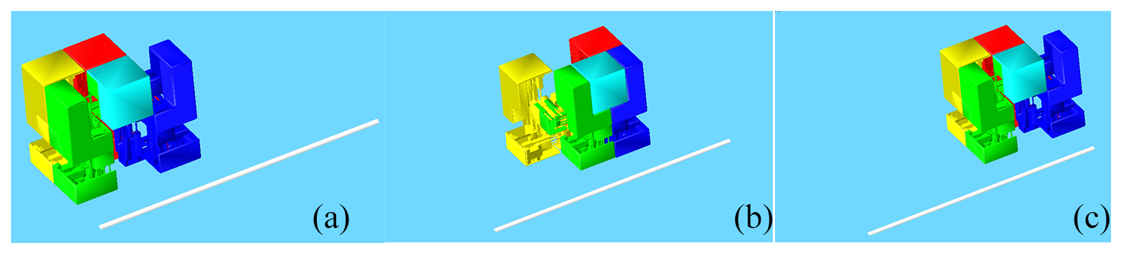
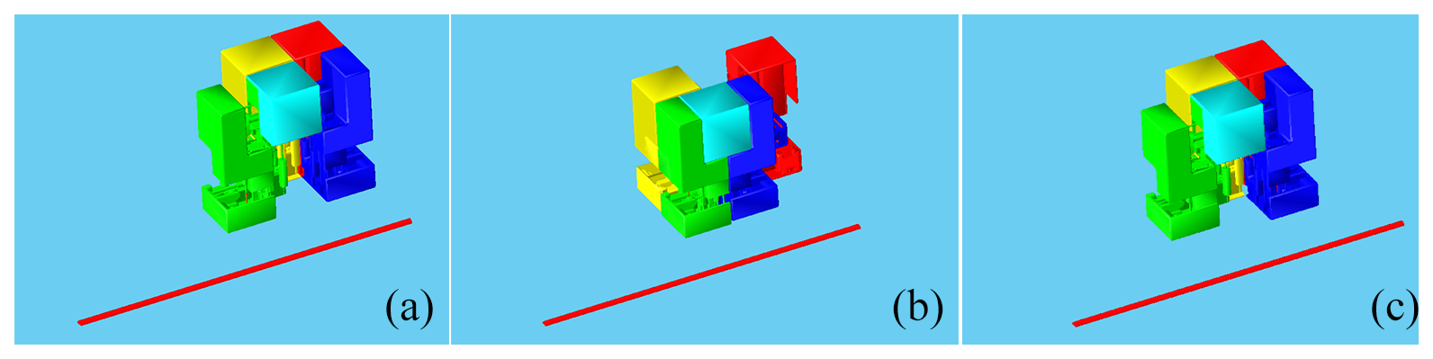
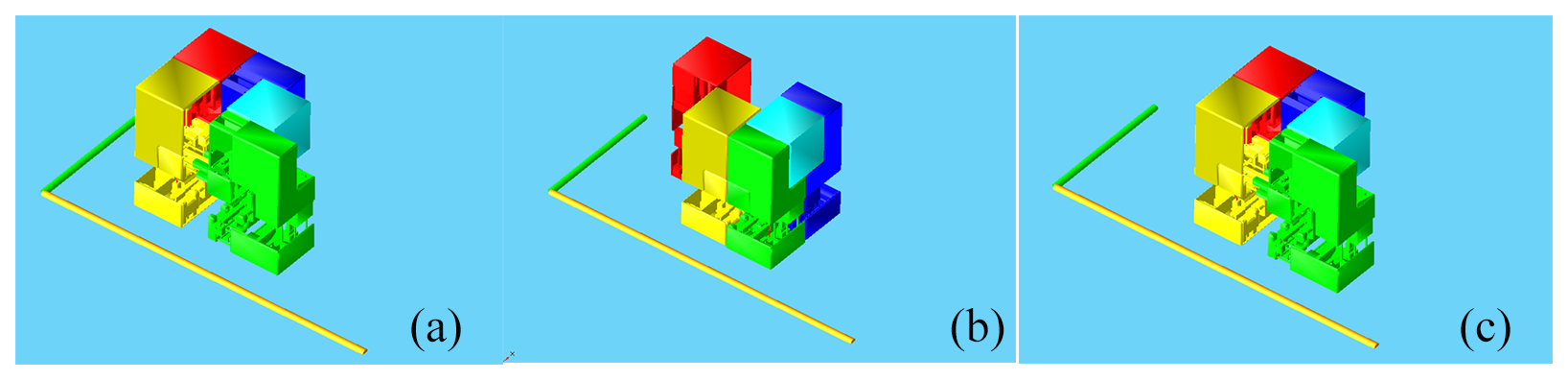
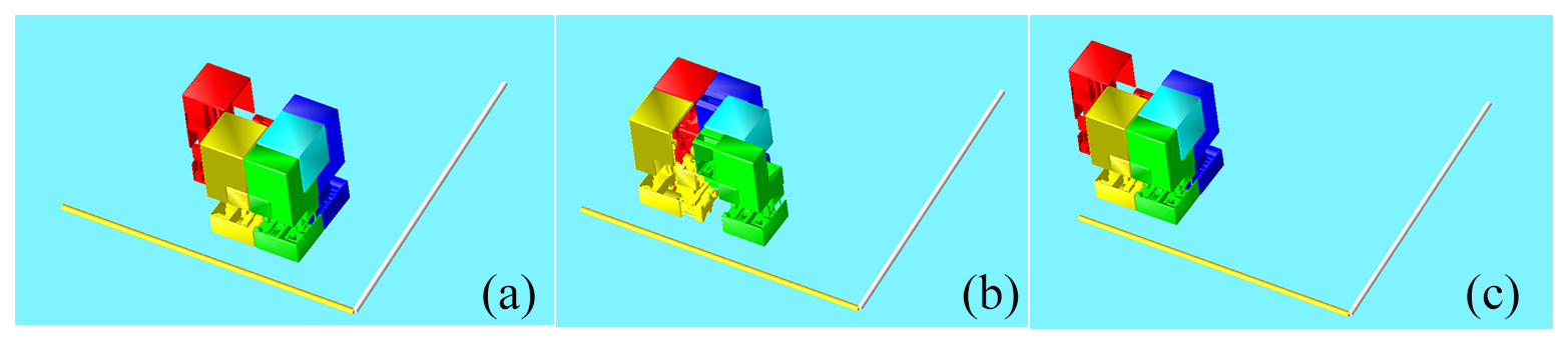
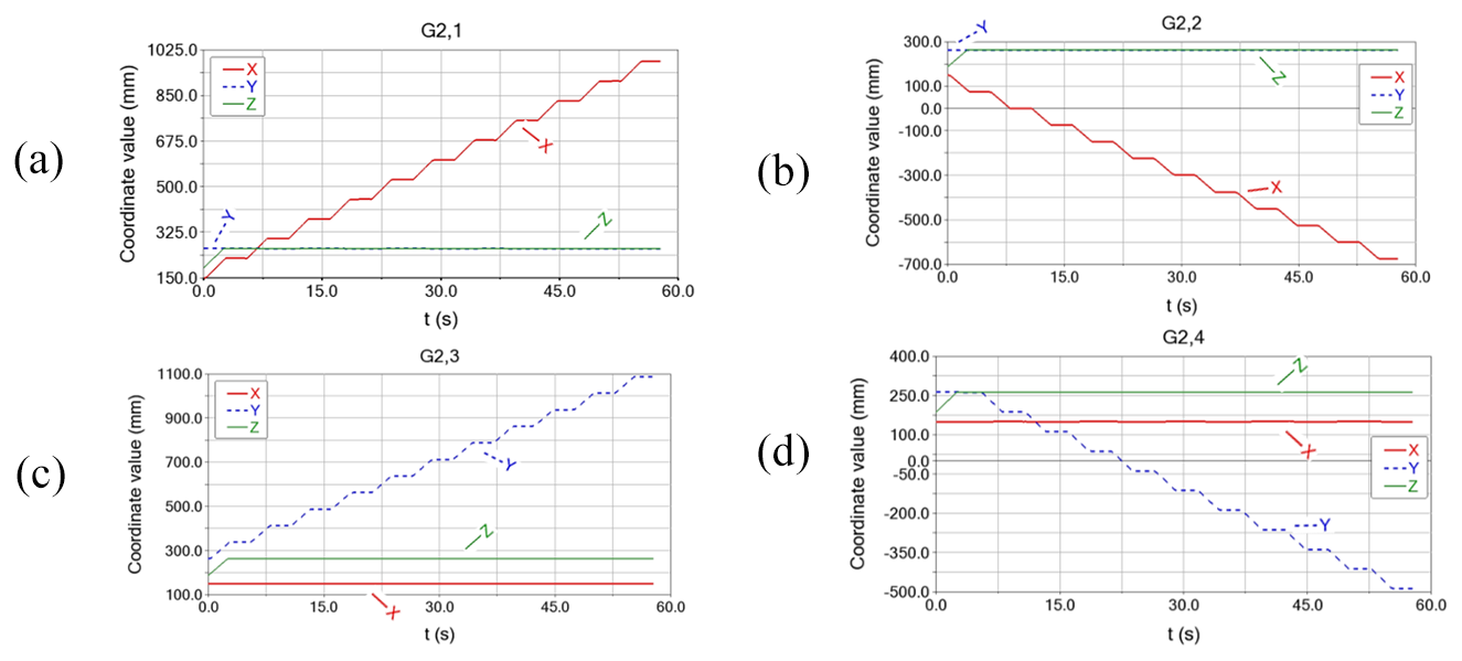
Figure 29 Change in the centroid coordinates of N₁₆ in plane motion. (a) G_2,1. (b) G_2,2. (c) G_2,3. (d) G_2,4.

4.3.2 HSCM rotary motion simulation

The movement of G_2,17 and G_2,18 during a simulation cycle is illustrated in Figs. 30 and 31, respectively. Subsequent to measuring and executing a rotation of 15°, G_2,17 and G_2,18 will each complete 10 cycles. The trajectory of the centre of mass of N₁₆ movement in the ground projection is depicted in Fig. 32. During each cycle (72 s), a rotation angle of 180° was achieved. The average rotational speed was measured to be 2.5° s⁻¹ in the clockwise direction and 2.5° s⁻¹ in the anticlockwise direction. The projection of the trajectory indicates that the robot's rotational motion planning is sustainable and stable.

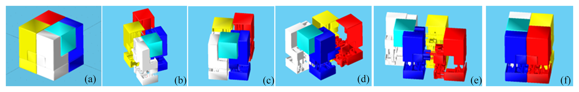
Figure 30 G_2,17 simulation. (a) t = 0 s. (b) t = 14.4 s. (c) t = 29 s. (d) t = 43.2 s. (e) t = 57.6 s. (f) t = 72 s.

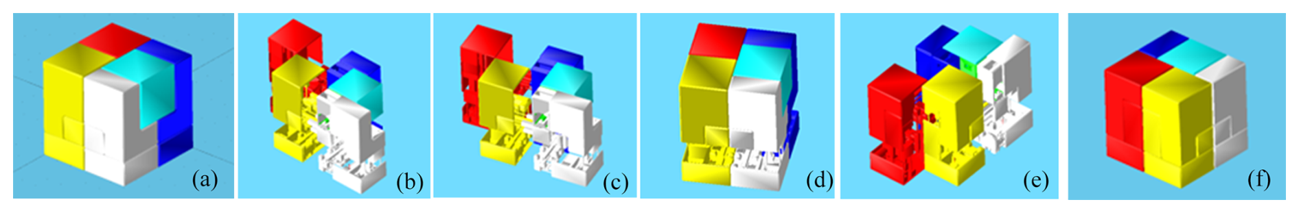
Figure 31 G_2,18 simulation. (a) t = 0 s. (b) t = 14.4 s. (c) t = 29 s. (d) t = 43.2 s. (e) t = 57.6 s. (f) t = 72 s.

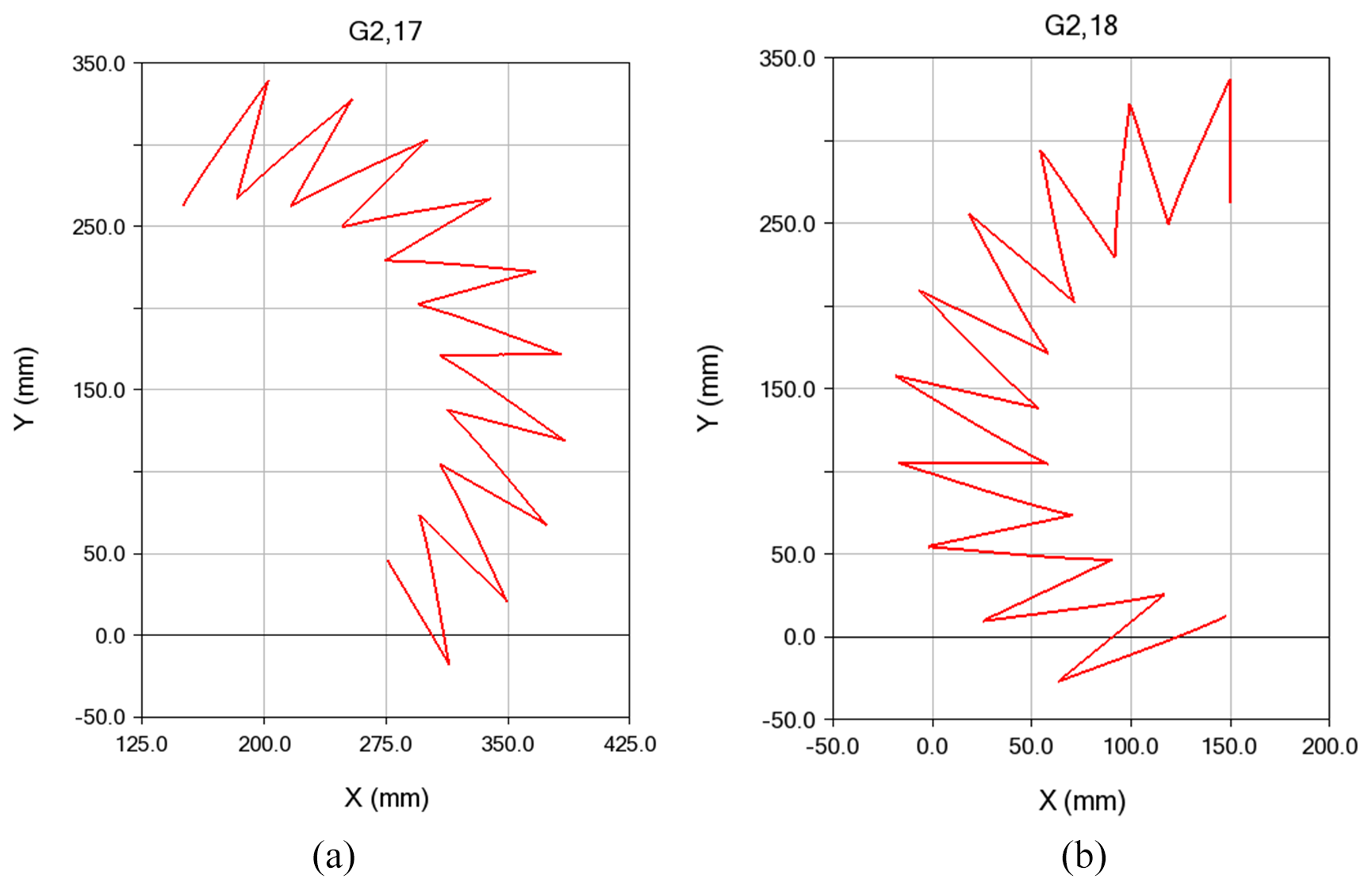
Figure 32 Trajectory projection of the centre of mass of N₁₆ in two rotational motions. (a) G_2,17. (b) G_2,18.

5 Prototypes and experiment

5.1 Construction of first-order robot prototype

Due to the specially designed and complex structure of the components, conventional machining methods proved both costly and technically challenging. To address this issue, several non-standard parts were fabricated using the laboratory's 3D printer.

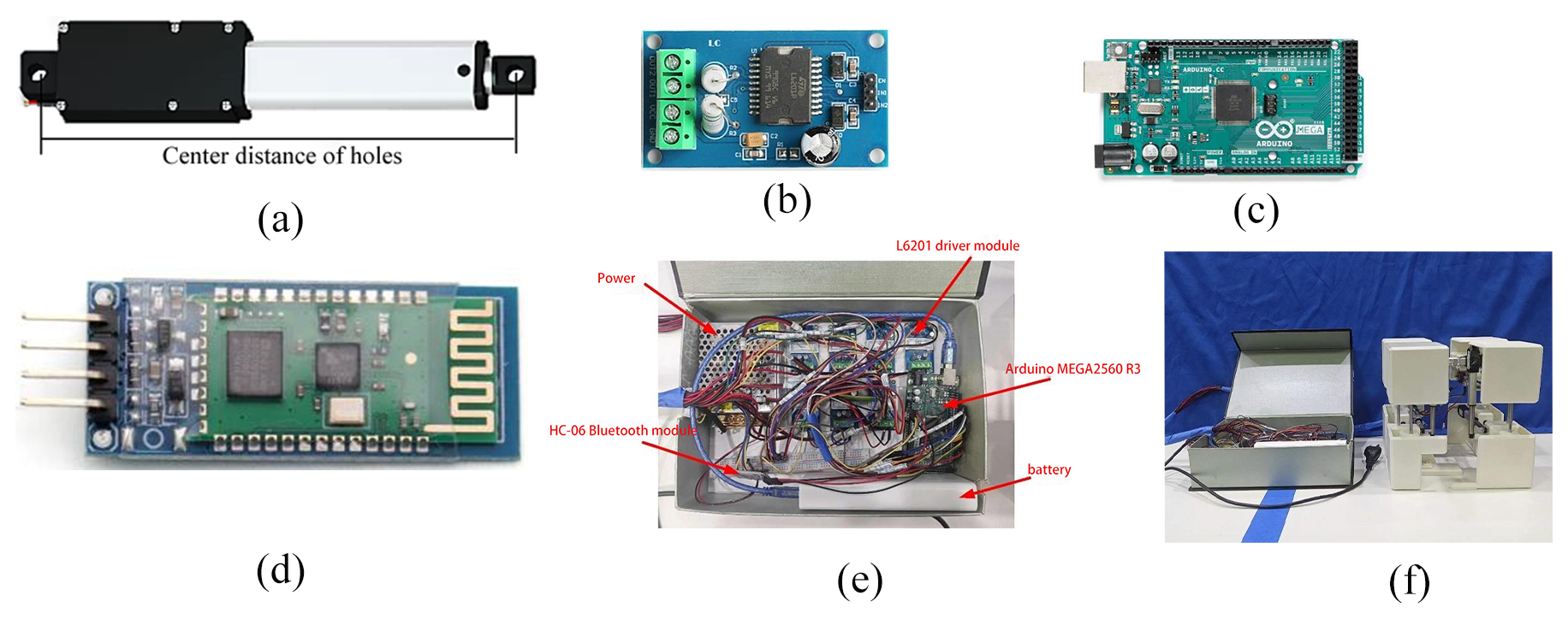
Figure 33 (a) DC motor pushrod. (b) L6201. (c) Arduino MEGA2560 R3. (d) HC-06 Bluetooth module. (e) Control box interior diagram. (f) The prototype.

DC motors were selected as the robot's drive system because they offer high efficiency under normal operating conditions, excellent speed regulation, a wide and smooth speed range, a simple structure, convenient control, and ease of maintenance. Furthermore, the linear relationship between input and output makes them highly suitable for precise actuation. Accordingly, DC motor pushrods were chosen as the driving mechanism, as shown in Fig. 33a. A pushrod length of 50 mm was determined to be sufficient for supporting various gaits of the mechanism.

The L6201 driver module was employed as the motor driver, as shown in Fig. 33b. This full-bridge driver chip is based on multi-source BCD (Bipolar, CMOS, DMOS) technology. It integrates independent DMOS field-effect transistors, CMOS circuits, and diodes on a single chip, thereby ensuring efficient and reliable motor control. The Arduino MEGA2560 R3 development board served as the main control unit, as shown in Fig. 33c. For wireless communication, HC-06 Bluetooth 2.0 slave modules were used, as illustrated in Fig. 33d.

Mechanical connections were reinforced by installing linear bearings and metal rods in the corresponding positions of eight 3D-printed connecting blocks. The metal rods acted as guide rails, ensuring precise alignment and improving structural strength. They were inserted into the linear bearings, and the DC motor pushrods were firmly attached to the connecting blocks to complete the assembly.

All electronic components – including the power supply, battery, Arduino MEGA2560 R3 development board, HC-06 Bluetooth module, and multiple L6201 driver modules – were integrated within a control box, as shown in Fig. 33e. Based on the designed gaits, a control program was developed and uploaded to the control board. Finally, the assembled mechanical structure was connected to the control box, yielding the complete prototype model shown in Fig. 33f.

5.2 HFCM linear mobility gait

In order to validate the HFCM structure and kinematic analysis, prototypes were developed and experiments were conducted. The geometry of the prototype is as follows (initial attitude): overall, a square with a prism length of 195 mm, m_i=218.75 g, $L_{AB}=L_{CD}=L_{DE}=L_{EF}=L_{GH}=\mathrm{90}$ mm, $L_{BC}=L_{FG}=\mathrm{80}$ mm, t=8 s, L₈=45 mm, u₁=8 mm, u₂=1 mm, u₃=8 mm, d₁=7.5 mm, d₂=65 mm, and Δl=50 mm. The course of the experimental forward walking gait along the x axis is shown in Fig. 34. The process of the forward walking gait along the y axis is shown in Fig. 35.

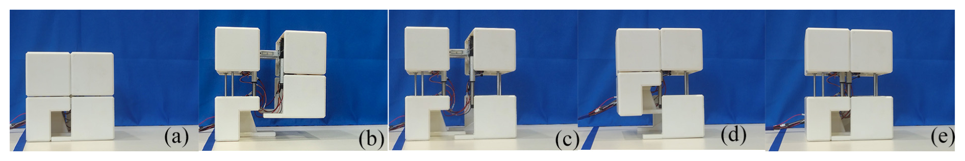
Figure 34 Positive movement of the prototype along the x axis. (a) Initial state. (b) Foot1 lifts. (c) Foot1 falls. (d) Foot2 lifts. (e) Foot2 falls.

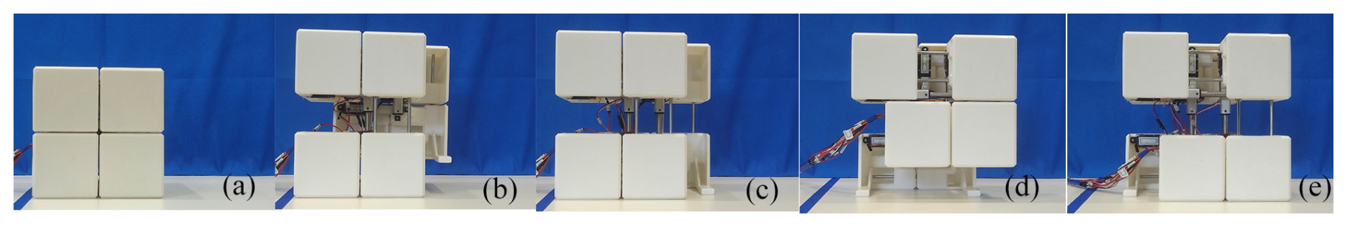
Figure 35 Positive movement of the prototype along the y axis. (a) Initial state. (b) Foot1 lifts. (c) Foot1 falls. (d) Foot2 lifts. (e) Foot2 falls.

Table 6 Gait feasibility analysis form.

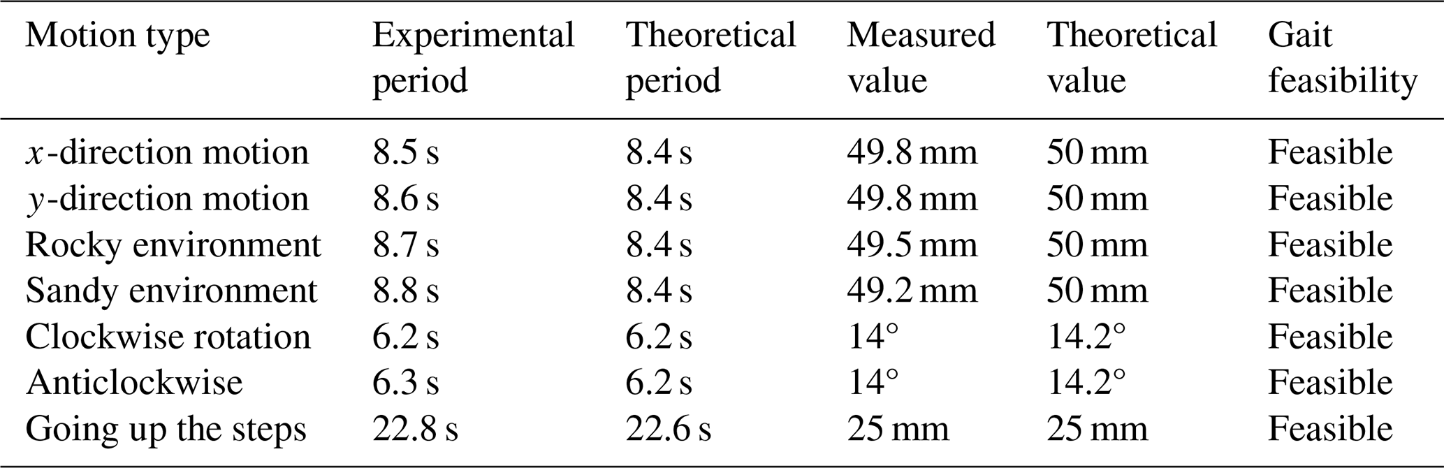
Figures 36 and 37 illustrate the linear locomotion of the HFCM in rocky and sandy environments. The experimental results demonstrate that both the stability and the errors of the HFCM remain within a controllable range, thereby validating the feasibility of the proposed gait. These findings provide a foundation for subsequent analysis and discussion of the mechanism's adaptability under varying terrain conditions.

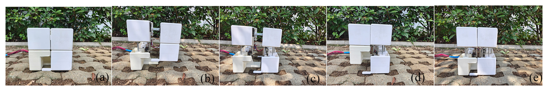
Figure 36 Linear locomotion of the HFCM in a rocky environment. (a) Initial state. (b) Foot1 lifts. (c) Foot1 falls. (d) Foot2 lifts. (e) Foot2 falls.

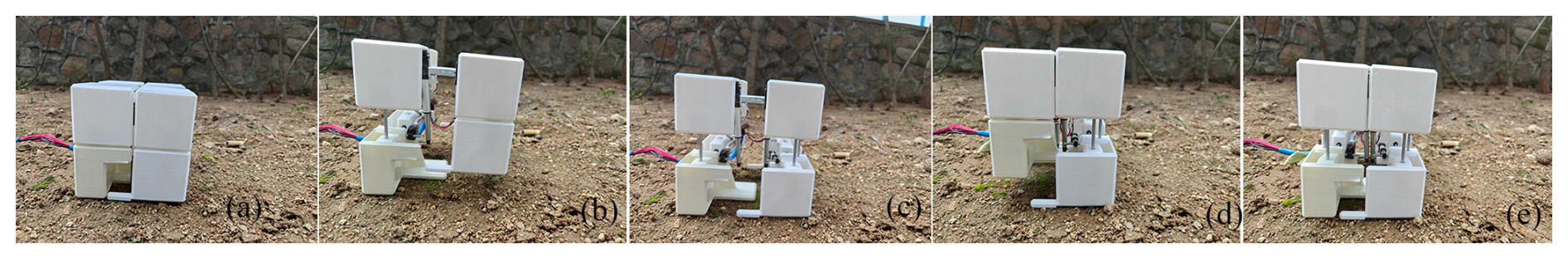
Figure 37 Linear locomotion of the HFCM in a sandy environment. (a) Initial state. (b) Foot1 lifts. (c) Foot1 falls. (d) Foot2 lifts. (e) Foot2 falls.

5.3 HFCM rotational gait

The process of rotational gait in the experiment is shown in Fig. 38. The angle of rotation of the HFCM in the clockwise direction after the completion of a rotational gait is shown in Table 4.

Figure 38 Clockwise rotation of the prototype. (a) Gait 1, (b) gait 2, (c) gait 3, (d) gait 1 top view, (e) gait 2 top view, and (f) gait 3 top view.

5.4 HFCM step-up gait

The process of rotational gait in the experiment is shown in Fig. 39. The mass of m_G is increased by 200 g. The step height is designed to be h = 25 mm, and the initial distance between the HFCM and the step is 0. The detailed feasibility analysis of the gait is summarized in Table 6.

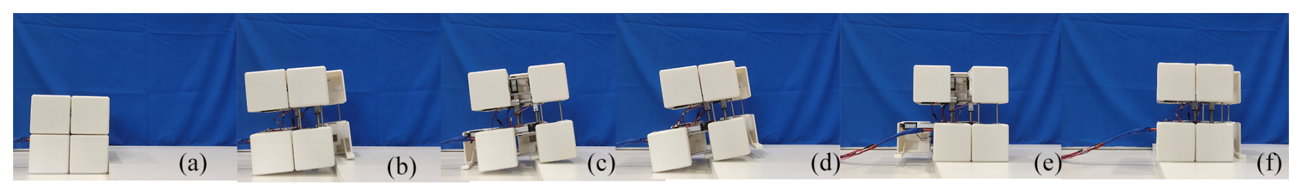
Figure 39 Going up the steps. (a) Initial pose. (b) Foot1 is out. (c) Foot2 is out. (d) Foot1 is out. (e) Foot2 takes a step up. (f) Gait completion.

6 Conclusion and Prospects

6.1 Sporting advantage

The space-filling property of the three-dimensional Hilbert curve enables compact deformation through the contraction and extension of joints, offering a unique advantage in confined environments. For example, the second-order mechanism can transform within a 64-cell cube, and its “fold–open” capability allows effective deployment in constrained settings such as pipelines and disaster ruins.

The Hilbert curve mechanism (HFCM) also supports diverse modes of movement. Dynamic gait adjustment allows adaptation to varying terrains. Alternating support feet enable stable planar walking. Step-crossing enhances its ability to overcome obstacles, while joint-driven actuation enables 360° in situ rotation.

Overall, the Hilbert curve mechanism represents a significant advancement in mobile robotics through its seamless integration of mathematical theory and engineering practice. By overcoming the conventional limitations of wheeled and legged robots, it demonstrates strong potential for applications in confined spaces, complex terrains, and specialized operational scenarios.

6.2 Application expansion

In the aftermath of a disaster, emergency response efforts primarily focus on rescue operations, including both post-disaster recovery and search-and-rescue missions. Conventional wheeled or legged robots are often hindered in confined environments such as ruins or pipelines due to structural limitations. By contrast, the Hilbert curve mechanism (HCM) offers the unique ability to transition between compact and expanded forms through continuous deformation. For example, it can contract to pass through narrow gaps in earthquake rubble and then expand to deploy sensors or rescue equipment. This adaptability significantly enhances the efficiency of search-and-rescue operations. The multi-legged support design further ensures stability on uneven terrain and enables navigation around complex obstacles.

In minimally invasive surgery, the flexibility of deformable mechanisms can be applied to retractable interventional instruments. HSCM-based serpentine robots, for instance, can be inserted into the body through natural cavities to perform precise operations in the heart or gastrointestinal tract. This approach reduces trauma, shortens recovery time, and minimizes surgical risk by avoiding rigid collisions with tissue.

In the context of spaceflight and deep-space exploration, where launch space is highly constrained, the folding property of the Hilbert curve mechanism allows significant volume reduction. For example, the HSCM can serve as a deformable arm for a Mars rover, unfolding into a three-dimensional structure after landing to integrate functions such as sampling and drilling. Its modular architecture also supports in-orbit self-repair and mission reconfiguration.

In industrial and agricultural inspection, the mechanism's adaptability is particularly valuable for navigating narrow passages and performing maintenance tasks in complex environments. The HFCM's straight-line extension enables non-destructive inspection within pipelines, while the HSCM's multi-step adaptability supports precision spraying or crop harvesting in greenhouses by traversing ridges and obstacles.

6.3 Conclusion

This paper introduces a novel integration of mathematical curves with mechanical structures, establishing a new paradigm for structural innovation. The proposed mobile mechanism is based on three-dimensional Hilbert curves. It incorporates seven straight lines connected by seven driven mobile joints, which enable the mechanism to expand and contract.

A comprehensive kinematic analysis is conducted to determine the parameters of the HFCM, followed by a detailed stability assessment. The biped demonstrates multiple gaits, including static walking, rotation, and stair climbing on flat surfaces. The feasibility of these motions is confirmed through both simulations and experiments.

The stability analysis is grounded in the zero moment point (ZMP) assumption, where acceleration and angular acceleration are neglected. This assumption is reasonable for static or quasi-static gaits at low speeds. However, it imposes limitations when the mechanism performs dynamic or high-speed motions. In such cases, the static ZMP approach may underestimate instability, making dynamic stability criteria more appropriate in the future.

To further validate the design, the HSCM model is implemented in ADAMS for motion simulation. Kinematic simulations are carried out using the derived mass configurations and motion planning. The results confirm the operational stability of all motion modes under a uniform mass configuration, thereby demonstrating the feasibility of the HSCM design.

6.4 Prospects

In future research, prototypes of second-order curve-based mechanisms will be further developed. Experimental studies will continue to verify the feasibility and stability of their structural configuration, mass distribution, and gait planning. These efforts will provide stronger evidence for the viability of mechanism designs derived from second-order three-dimensional Hilbert curves.

The extension of this mechanism to higher-order curves will require more driving joints. Under such conditions, traditional centralized control systems are likely to encounter delays and coupling problems. To overcome these challenges, distributed control architectures that combine edge computing with real-time path gauging will need to be developed. Such approaches will enable dynamic joint coordination and ensure reliable performance in complex environments.

At the same time, higher-order mechanisms will inevitably increase system mass. This will create a demand for lightweight materials and optimized structural designs that can enhance stiffness without compromising mobility. The integration of energy recovery systems – such as springs that store and release energy during deformation – will also be essential to improving overall efficiency.

From the perspective of motion stability, current zero moment point (ZMP) analyses are limited to static gaits. Future work will incorporate dynamic stability analysis to account for inertial effects and angular accelerations. Moving beyond the static ZMP assumption will make it possible to evaluate gait robustness under dynamic conditions and ensure stable locomotion in more complex and high-speed scenarios. For example, fuzzy PID controllers could be introduced into Hilbert curve-based mechanisms to compensate for terrain disturbances in real time and enhance adaptability.

Ultimately, Hilbert curve mechanisms demonstrate strong potential to transcend the morphological constraints of conventional mobile robots by integrating mathematical theory with engineering practice. With continuous progress in control strategies, material technologies, and interdisciplinary applications, these mechanisms are expected to evolve from laboratory validation toward real-world deployment, establishing a new paradigm for the development of intelligent robotic systems.

Appendix A: Symbol implication

A, B, C, D, E, F, G, H	Eight nodes of the HFCM / centre of mass of each connecting rod
Ni (i=1, 2, …, 31)	HSCM's 31 node connection block
hi (i=1, 2, 3, 4, 5)	Connection point of support rods to the base plate in HFCM support structures
k1, k2, k3	HFCM support base plate end point centre
LAB, LBC, LCD, LDE, LEF, LFG, LGH	Distance between nodes in the initial state of the HFCM
Li (i=1, 2, 3, 4, 5, 6, 7)	Distance between neighbouring centres of mass in HFCM to point G
l1	Length of support rods of the support mechanism on both sides of Foot1 and Foot2 in the HFCM
l2	Length of support rods for intermediate support mechanism of Foot2 in the HFCM
u1	Length of base plate on both sides of Foot1 in the HFCM
u2	Length of base plate on both sides of Foot2 in the HFCM
u3	Length of intermediate base plate of Foot2 in the HFCM
d1	Width of Foot1 and Foot2 base plates on both sides of the HFCM
d2	Width of intermediate base plate of Foot2 in the HFCM
Δl	HFCM travel distance per travelling joint
t1	HFCM time to complete t1 extension/retraction strokes per joint
θ	Angle between the support bar and the base plate on both sides of Foot1 and Foot2 in the HFCM
CM	Centre of mass
CMx, CMy, CMz	HFCM coordinates of the centre of mass in the direction of the x, y, and z axes
CM2	HSCM centre of mass
$x_{{\mathrm{CM}}_{\mathrm{2}}}^g$, $y_{{\mathrm{CM}}_{\mathrm{2}}}^g$, $z_{{\mathrm{CM}}_{\mathrm{2}}}^g$	HSCM coordinates of the centre of mass in the x, y, and z directions in the coordinate system g-xyz
ZMP	Zero moment point
xZMP, yZMP	ZMP coordinates in the x, y directions
mi	Quality of connecting blocks at each node of the HFCM
Mi	Quality parameters of HSCM connecting blocks for each node
Ji	Moment of inertia (mechanics)
αi	Angular acceleration
${\ddot{x}}_i$, ${\ddot{y}}_i$, ${\ddot{z}}_i$	Acceleration of each centre of mass in the x, y, and z directions
gz	Component of gravitational acceleration in the z-axis direction
O-xyz	Fixed coordinate system (terrestrial coordinate system)
Si-xyz	Dynamic coordinate system
g-xyz	Dynamic coordinate system
${}_{\mathrm{CM}}^{O}P$	HFCM chiral coordinates of the centre of mass CM in the O-xyz coordinate system
${}_{h_i}^{\mathrm{CM}}P$	Initial coordinates of point hi in the CM-xy coordinate system
$T\left({}_{\mathrm{CM}}^{O}P\right)$	Translation transform matrix
${}_{h_i}^{\mathrm{CM}}R(Z,\mathit{\alpha })$	Rotational transformation matrix around the z axis
${}_{A_i}^O{P}_j$, ${}_{e_i}^O{P}_j$	Coordinates of points Ai, ei in the O-xyz coordinate system at step j
ΔAi, Δei	Relative displacement of points Ai, ei in the g-xyz coordinate system
${}_{S_i}^{O}R$, ${}_g^{S_i}R$	Rotation matrix between coordinate systems
${\mathit{\psi }}_j^{G_{\mathrm{2},i}}$	Axis of rotation of gait G2,i at step j
${\mathit{\xi }}_j^{G_{\mathrm{2},i}}$	Angle of rotation of gait G2,i at step j
G2,1–G2,18	The 18 basic gaits of HSCM