Dimensional synthesis of a spatial revolute–revolute–spherical–cylindrical (RRSC) mechanism for motion generation

This paper presents a dimensional synthesis method of a spatial revolute–revolute–spherical–cylindrical (RRSC) rigid-body guidance mechanism for motion generation. The inputs into the mechanism, namely the prescribed spatial poses, are analysed, revealing that, after two steps of coordinate transformation, the corresponding coupler points lie on a circle. Based on this finding, an input angle determination method is proposed. The design process for the 21 geometric parameters is then decomposed into four steps: first, obtaining the installation angles, the initial input angle, and the angle between the rotation axes of the input link and coupler link; second, determining the basic dimensional types; third, calculating the remaining parameters based on the relationship between the prescribed poses and the generated coupler points; and, fourth, optimizing the mechanism parameters obtained in the first three steps. This approach assumes rigid links and ideal joints. Through this four-step approach, the design efficiency is significantly improved by reducing the dimensionality of the design problem. Notably, the method accommodates both prescribed- and unprescribed-timing design requirements. Its practicality and effectiveness are demonstrated through numerical examples.

1 Introduction

The spatial revolute–revolute–spherical–cylindrical (RRSC) mechanism has several practical applications in industry due to its ability to generate complex spatial motion with relatively few joints. For example, it can be used in robotic wrists to smoothly and accurately track curved surfaces, as well as in packaging machinery to achieve three-dimensional positioning and orientation adjustments of objects. Furthermore, this mechanism is suitable for aircraft landing gear systems, large-scale antenna adjustment mechanisms, and more. Additionally, the spatial RRSC mechanism holds broad application prospects in fields such as aerospace and medical rehabilitation. Synthesizing such a mechanism is important because it allows engineers to systematically design a linkage that meets specific motion requirements, such as following a desired pose in space. This process helps optimize the mechanism's performance, improve its efficiency, and reduce development time and physical prototyping costs.

The dimensional synthesis of mechanisms represents a classical yet persistent challenge in mechanical design. The planar linkage mechanisms have been well-studied, and numerous effective synthesis methods exist, such as analytical methods (Bai and Angeles, 2015; Liu and Yu, 2022), optimization methods (Kim et al., 2016; Kafash and Nahvi, 2017), and atlas methods (Liu et al., 2025), along with dedicated design software (Purwar et al., 2017). However, compared with planar linkages, spatial linkage mechanisms remain significantly more difficult to address. This complexity arises from their intricate spatial geometries, higher number of design variables, and strong nonlinearities, as well as the difficulty in satisfying constraints simultaneously.

The analytical method can establish a system of equations based on the given design conditions and then realize the dimensional synthesis of the linkage mechanism by solving the nonlinear system of equations. Han and Cao (2019) investigated the problem of motion generation for the spatial revolute–cylindrical–cylindrical–cylindrical (RCCC) mechanism and proposed a synthesis method for the four-position design requirements. Cervantes-Sánchez et al. (2014) investigated the problem of synthesizing the six-position function of a spatial revolute–revolute–revolute–cylindrical–revolute (RRRCR) mechanism and developed a system of nonlinear equations for solving the dimensional parameters of the desired mechanism. Wang et al. (2019) proposed a synthesis method for motion generation of a spherical four-bar mechanism with four-position design requirements based on Burmester's theory. Bai (2021) and Bai et al. (2022) established a set of algebraic equations for the dimensional parameters and installation angle parameters of the mechanism with the help of parametric coordinates and provided a path synthesis method for spherical linkage and spatial RCCC mechanisms with fewer positional design requirements. Cao and Han (2020) investigated the rigid-body guidance synthesis problem of the spatial helical–cylindrical–cylindrical–cylindrical (HCCC) mechanism and proposed a step-by-step design method for the space HCCC rigid-body guidance mechanism with four-position design requirements. The advantage of the analytical method is that it can precisely determine the geometric parameters of the linkage mechanism based on design requirements. However, it is also limited by the fact that the number of prescribed exact positions cannot exceed the number of available equations. As a result, this method is unable to solve dimensional synthesis problems involving a broad range of multi-position design requirements, which are commonly encountered in engineering practice.

The numerical atlas method is one of the primary techniques used in mechanism dimensional synthesis to meet multiple position design requirements. This method offers advantages such as broad applicability, repeatability, stability, reliability, and ease of controlling the synthesized trend. Its key challenge involves the extraction of characteristic parameters. McGarva (1994) normalized the harmonic parameters to eliminate the effects of translations and rotations of the linkage curves and proposed a method for describing the output linkage curves of a planar four-bar mechanism using these parameters. Mullineux (2011) proposed using a Fourier series to describe the output trajectory curve of a spherical linkage mechanism and to extract its characteristic parameters. Li et al. (2016) proposed a motion-fitting scheme in Fourier representation for the dimensional synthesis of motion generation for four-bar mechanisms. Sharma et al. (2019) introduced an analytical approach leveraging Fourier approximation to address the Alt–Burmester problem, effectively simplifying it into a pure motion synthesis issue. Sun et al. (2015) proposed a wavelet feature parameter method for the dimensional synthesis of linkage mechanisms, which enables the solution of the dimensional synthesis problem for planar and spherical linkage mechanisms with arbitrary design intervals. Zhang et al. (2022) investigated the problem of path generation of a spherical five-bar mechanism based on a numerical atlas method. Since the numerical atlas method is a dimensional synthesis technique based on exhaustive methods and fuzzy recognition theory, it necessitates the pre-establishment of a vast numerical atlas database. This approach presents issues such as significant space occupation by the atlas database, a protracted synthesis process, and diminished efficiency in matching and recognition. Moreover, achieving highly accurate synthesis results with a static numerical atlas database is challenging due to the discrete nature of the mechanism parameters contained within it.

Compared to the numerical atlas method, the optimization method is less time-consuming and more efficient in performing matching and identification. Zhao et al. (2016) utilized a greedy search algorithm to address the motion generation problem involving multiple position design requirements. Peón-Escalante et al. (2020) established an optimization objective function that incorporates Euclidean distance error and utilizes a differential evolution algorithm to achieve path synthesis for planar and spherical Stephenson-III-type six-bar mechanisms, meeting multiple position design requirements. Liu et al. (2023) proposed a dimensional synthesis method for motion generation of a spatial revolute–revolute–spherical–spherical (RRSS) mechanism using a genetic algorithm. Lee et al. (2020) proposed a general optimization model for a spatial multi-loop revolute–spherical–spherical–revolute–spherical–spherical linkage. Building on this, they calculated the dimensions of the mechanism necessary to approximate precise positions. Hernández et al. (2021) proposed a method for synthesizing the trajectories of a planar four-bar mechanism, which is based on the gradient method and uses the mechanism's input angle as design variables, to meet 18 specified position design requirements. Torres-Moreno et al. (2022) implemented a solution to the trajectory synthesis problem for a planar four-bar mechanism with multiple position design requirements using a teach-and-learn optimization algorithm. They also developed an associated computer-aided design programme. The optimization method can yield a highly accurate design solution in a very short design cycle when the initial values of the optimization variables are good. Additionally, this method can be applied to solve dimension synthesis problems with unprescribed-timing design requirements. However, the optimization method cannot avoid the issue that the synthesis results are significantly influenced by the initial values of the optimization variables, the choice of optimization method, and the objective function. Essentially, it is a global optimization problem involving multi-dimensional variables. Therefore, when applying the optimization method to solve the dimensional synthesis problem of a linkage mechanism with multiple positions and unprescribed-timing design requirements, it is challenging to guarantee the convergence of the optimization method and the stability of the design outcomes.

In this paper, a method for dimensional synthesis that integrates the numerical atlas method with the optimization method to achieve an accurate design solution is proposed. Compared to existing spatial mechanism motion synthesis methods, the method proposed in this paper employs a step-by-step approach to overcome the deficiencies of the numerical atlas method, which requires establishing a large numerical atlas database. It also retains the advantages of the numerical atlas method, such as conceptual clarity, simplicity of calculation, and high accuracy in analysis methods. Finally, the geometric parameters of the mechanism are optimized using a genetic algorithm, which enhances synthesis accuracy and ensures the stability of the design outcomes. This paper contributes three principal insights to the field of spatial mechanism synthesis. First, it establishes a systematic methodology for determining input angles for RRSC rigid-body guidance mechanisms, overcoming the critical coupling constraint that necessitates the concurrent optimization of input angles and linkage dimensional parameters. Second, it strategically decomposes the complex 21-geometric-parameter design problem into three cascaded optimization stages, achieving dimensionality reduction through controlled variable allocation at each phase. Most notably, we demonstrate the first successful realization of non-prescribed-timing motion generation for spatial RRSC mechanisms. The optimized geometric parameters exhibit pose quantity invariance; this crucial property ensures solution robustness even when subjected to escalating positional constraints.

The remainder of this paper is organized as follows. In Sect. 2, the mathematical model of a spatial RRSC rigid-body guidance mechanism is established. A processing method is proposed to obtain the feature coupler circles. Then, an input angle determination method for a spatial RRSC mechanism in a standard installation position is presented. In Sect. 3, the input angle determination method is extended to spatial RRSC mechanisms in general installation positions, providing a foundation for solving the 21-geometric-parameter design process, which is divided into three steps. In Sect. 4, the specific design steps for the dimensional synthesis of spatial RRSC rigid-body guidance mechanisms are presented. In Sect. 5, two examples are provided to demonstrate the efficacy of the proposed method.

Figure 1 A spatial RRSC rigid-body guidance mechanism in a standard installation position.

2 Feature coupler circles of a spatial RRSC mechanism

2.1 Mathematical model of a spatial RRSC rigid-body guidance mechanism

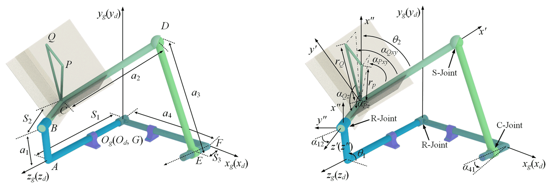
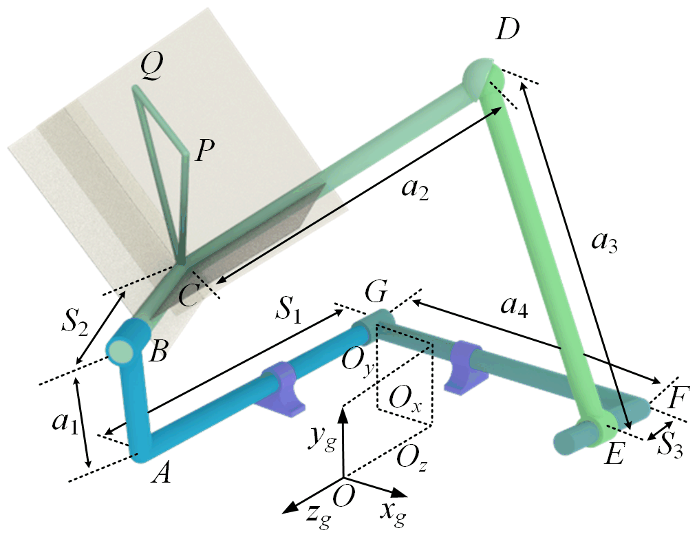
Figure 1 shows a single-degree-of-freedom RRSC spatial mechanism in a standard installation position. Here, AB is the input link, CD is the coupler link, DE is the driven link, and FG is the frame. The lengths of the links (AB, CD, DE, FG, GA, BC, and EF) are denoted by a₁, a₂, a₃, a₄, S₁, S₂, and S₃, respectively, as depicted in Fig. 1 O_d−x_dy_dz_d is a coordinate system attached to the frame, where the coordinate origin O_d aligns with point G of the frame, the z_d axis aligns with the axis of rotation of the input link, and the x_d axis coincides with the vertical line of the z_d axis passing through the point F. Two additional coordinate systems, O^′-$x^{\prime }{y}^{\prime }{z}^{\prime }$ and O^′′-$x^{\prime \prime }{y}^{\prime \prime }{z}^{\prime \prime }$, are attached to the input link and the coupler link, respectively. In the coordinate system O^′-$x^{\prime }{y}^{\prime }{z}^{\prime }$, the origin O^′ coincides with the point C, the z^′ axis aligns with the axis of rotation of the coupler link, and the x^′ axis aligns with the vertical line of the z^′ axis passing through the centre of the spherical pair D. For the coordinate system O^′′-$x^{\prime \prime }{y}^{\prime \prime }{z}^{\prime \prime }$, the origin O^′′ coincides with point B, the z^′′ axis aligns with the z^′ axis, and the x^′′ axis aligns with AB. θ represents the angle between the x^′ axis and the x^′' axis, defined as the coupler angle. α₁₂ is the angle between the rotation axis of the input link and the rotation axis of the coupler link. α₄₁ is the angle between the rotation axis of the driven link and the rotation axis of the input link. The directions of α₁₂ and α₄₁ are determined by the right-hand rule. For α₁₂, the thumb is aligned along the common normal between the two axes (AB) pointing from A to B; for α₄₁, the thumb is aligned along the common normal between the two axes (FG) pointing from F to G. The curl of the fingers indicates the positive directions. θ₁ is the input angle. The position of point P is determined by the three parameters r_P, α_Pxy, and α_Pz. α_Pxy is the angle between the x^′ axis and the projection of CP on the $x^{\prime }{O}^{\prime }{y}^{\prime }$ plane, while α_Pz is the angle between CP and the z^′ axis. r_P is the length of CP. Similarly, the position of point Q is determined by the three parameters r_Q, α_Qxy, and α_Qz. α_Qxy is the angle between the x^′ axis and the projection of CQ on the $x^{\prime }{O}^{\prime }{y}^{\prime }$ plane, and α_Qz is the angle between CQ and the z^′ axis. r_Q is the length of CQ. O_g−x_gy_gz_g is a global coordinate system. For a spatial RRSC rigid-guidance mechanism in a standard installation position, the coordinates O_d−x_dy_dz_dcoincide with O_g−x_gy_gz_g. PQ is a guidance line – a fixed reference line on the coupler link that defines the body's precise position and orientation at each prescribed point along its path. According to the geometric relationship between each link, the positions of points P and Q in the global coordinate system O_g−x_gy_gz_g can be expressed as follows:

$$\begin{array}{}\text{(1)}& {\displaystyle }\begin{array}{rl}& \left[\begin{array}{c}{x}_P\\ y_P\\ z_P\end{array}\right]\\ & =\left[\begin{array}{c}\left[r_P\sin {\mathit{\alpha }}_{Pz}\cos ({\mathit{\alpha }}_{Pxy}-{\mathit{\theta }}_{\mathrm{2}})+a_{\mathrm{1}}\right]\cos {\mathit{\theta }}_{\mathrm{1}}+\left[\left(r_P\cos {\mathit{\alpha }}_{Pz}-S_{\mathrm{2}}\right)\sin {\mathit{\alpha }}_{\mathrm{12}}-\right.\left.r_P\sin {\mathit{\alpha }}_{Pz}\cos {\mathit{\alpha }}_{\mathrm{12}}\sin ({\mathit{\alpha }}_{Pxy}-{\mathit{\theta }}_{\mathrm{2}})\right]\sin {\mathit{\theta }}_{\mathrm{1}}\\ \left[r_P\sin {\mathit{\alpha }}_{Pz}\cos ({\mathit{\alpha }}_{Pxy}-{\mathit{\theta }}_{\mathrm{2}})+a_{\mathrm{1}}\right]\sin {\mathit{\theta }}_{\mathrm{1}}-\left[\left(r_P\cos {\mathit{\alpha }}_{Pz}-S_{\mathrm{2}}\right)\sin {\mathit{\alpha }}_{\mathrm{12}}-\right.\left.r_P\sin {\mathit{\alpha }}_{Pz}\cos {\mathit{\alpha }}_{\mathrm{12}}\sin ({\mathit{\alpha }}_{Pxy}-{\mathit{\theta }}_{\mathrm{2}})\right]cos{\mathit{\theta }}_{\mathrm{1}}\\ \left(r_P\cos {\mathit{\alpha }}_{Pz}-S_{\mathrm{2}}\right)\cos {\mathit{\alpha }}_{\mathrm{12}}+r_P\sin {\mathit{\alpha }}_{Pz}\sin \left({\mathit{\alpha }}_{Pxy}-{\mathit{\theta }}_{\mathrm{2}}\right)\sin {\mathit{\alpha }}_{\mathrm{12}}+S_{\mathrm{1}}\end{array}\right],,\end{array}\text{(2)}& {\displaystyle }\begin{array}{rl}& \left[\begin{array}{c}{x}_Q\\ y_Q\\ z_Q\end{array}\right]\\ & =\left[\begin{array}{c}\left[r_Q\sin {\mathit{\alpha }}_{Qz}\cos ({\mathit{\alpha }}_{Qxy}-{\mathit{\theta }}_{\mathrm{2}})+a_{\mathrm{1}}\right]\cos {\mathit{\theta }}_{\mathrm{1}}+\left[\left(r_Q\cos {\mathit{\alpha }}_{Qz}-S_{\mathrm{2}}\right)\sin {\mathit{\alpha }}_{\mathrm{12}}-\right.\left.r_Q\sin {\mathit{\alpha }}_{Qz}\cos {\mathit{\alpha }}_{\mathrm{12}}\sin ({\mathit{\alpha }}_{Qxy}-{\mathit{\theta }}_{\mathrm{2}})\right]\sin {\mathit{\theta }}_{\mathrm{1}}\\ \left[r_Q\sin {\mathit{\alpha }}_{Qz}\cos ({\mathit{\alpha }}_{Qxy}-{\mathit{\theta }}_{\mathrm{2}})+a_{\mathrm{1}}\right]\sin {\mathit{\theta }}_{\mathrm{1}}-\left[\left(r_Q\cos {\mathit{\alpha }}_{Qz}-S_{\mathrm{2}}\right)\sin {\mathit{\alpha }}_{\mathrm{12}}-\right.\left.r_Q\sin {\mathit{\alpha }}_{Qz}\cos {\mathit{\alpha }}_{\mathrm{12}}\sin ({\mathit{\alpha }}_{Qxy}-{\mathit{\theta }}_{\mathrm{2}})\right]\cos {\mathit{\theta }}_{\mathrm{1}}\\ \left(r_Q\cos {\mathit{\alpha }}_{Qz}-S_{\mathrm{2}}\right)\cos {\mathit{\alpha }}_{\mathrm{12}}+r_Q\sin {\mathit{\alpha }}_{Qz}\sin \left({\mathit{\alpha }}_{Qxy}-{\mathit{\theta }}_{\mathrm{2}}\right)\sin {\mathit{\alpha }}_{\mathrm{12}}+S_{\mathrm{1}}\end{array}\right]..\end{array}\end{array}$$

Based on the geometric relationships among the four links of the spatial RRSC rigid-body guidance mechanism, the distance from point D to point F can be derived using the Pythagorean theorem:

$$\begin{array}{}\text{(3)}& L_{DF}={\left(x_D-x_F\right)}^{\mathrm{2}}+{\left(y_D-y_F\right)}^{\mathrm{2}}+{\left(z_D-z_F\right)}^{\mathrm{2}}=a_{\mathrm{3}}^{\mathrm{2}}+S_{\mathrm{3}}^{\mathrm{2}},\end{array}$$

where x_D, y_D, and z_D are the coordinates of point D, and x_F, y_F, and z_F are the coordinates of point F. In the coordinate system O_g−x_gy_gz_g, x_D, y_D, and z_D can be expressed as follows:

$$\begin{array}{}\text{(4)}& \left[\begin{array}{c}{x}_D\\ y_D\\ z_D\end{array}\right]=\left[\begin{array}{c}{a}_{\mathrm{2}}\cos {\mathit{\theta }}_{\mathrm{2}}\cos {\mathit{\theta }}_{\mathrm{1}}+a_{\mathrm{1}}\cos {\mathit{\theta }}_{\mathrm{1}}-S_{\mathrm{2}}\sin {\mathit{\alpha }}_{\mathrm{12}}\sin {\mathit{\theta }}_{\mathrm{1}}+a_{\mathrm{2}}\sin {\mathit{\theta }}_{\mathrm{2}}\cos {\mathit{\alpha }}_{\mathrm{12}}\sin {\mathit{\theta }}_{\mathrm{1}}\\ a_{\mathrm{2}}\cos {\mathit{\theta }}_{\mathrm{2}}\sin {\mathit{\theta }}_{\mathrm{1}}+a_{\mathrm{1}}\sin {\mathit{\theta }}_{\mathrm{1}}+S_{\mathrm{2}}\sin {\mathit{\alpha }}_{\mathrm{12}}\cos {\mathit{\theta }}_{\mathrm{1}}-a_{\mathrm{2}}\sin {\mathit{\theta }}_{\mathrm{2}}\cos {\mathit{\alpha }}_{\mathrm{12}}\cos {\mathit{\theta }}_{\mathrm{1}}\\ S_{\mathrm{1}}-S_{\mathrm{2}}\cos {\mathit{\alpha }}_{\mathrm{12}}-a_{\mathrm{2}}\sin {\mathit{\theta }}_{\mathrm{2}}\sin {\mathit{\alpha }}_{\mathrm{12}}\end{array}\right].\end{array}$$

x_F, y_F, and z_F can be expressed as follows:

$$\begin{array}{}\text{(5)}& \left[\begin{array}{c}{x}_F\\ y_F\\ z_F\end{array}\right]=\left[\begin{array}{c}{a}_{\mathrm{4}}\\ \mathrm{0}\\ \mathrm{0}\end{array}\right].\end{array}$$

By projecting the vector loop closure ABCDEFG onto EF, the expression for the mechanism parameter S₃ can be obtained as follows:

$$\begin{array}{}\text{(6)}& \begin{array}{rl}{S}_{\mathrm{3}}& =a_{\mathrm{2}}\cos {\mathit{\theta }}_{\mathrm{2}}\sin {\mathit{\theta }}_{\mathrm{1}}\sin {\mathit{\alpha }}_{\mathrm{41}}{a}_{\mathrm{2}}\sin {\mathit{\theta }}_{\mathrm{2}}(\sin a_{\mathrm{12}}\cos {\mathit{\alpha }}_{\mathrm{41}}+\cos a_{\mathrm{12}}\\ & \cos {\mathit{\theta }}_{\mathrm{1}}\sin {\mathit{\alpha }}_{\mathrm{41}})+(a_{\mathrm{1}}\sin {\mathit{\theta }}_{\mathrm{1}}+S_{\mathrm{2}}\sin {\mathit{\alpha }}_{\mathrm{12}}\cos {\mathit{\theta }}_{\mathrm{1}})\sin {\mathit{\alpha }}_{\mathrm{41}}+S_{\mathrm{1}}\\ & \cos {\mathit{\alpha }}_{\mathrm{41}}{S}_{\mathrm{2}}\cos a_{\mathrm{12}}\cos {\mathit{\alpha }}_{\mathrm{41}}.\end{array}\end{array}$$

Substituting Eqs. (4) to (6) into Eq. (3) yields

$$\begin{array}{}\text{(7)}& \begin{array}{rl}{w}_{\mathrm{1}}{\cos }^{\mathrm{2}}{\mathit{\theta }}_{\mathrm{2}}& +w_{\mathrm{2}}{\sin }^{\mathrm{2}}{\mathit{\theta }}_{\mathrm{2}}+w_{\mathrm{3}}\sin {\mathit{\theta }}_{\mathrm{2}}\cos {\mathit{\theta }}_{\mathrm{2}}+w_{\mathrm{4}}\sin {\mathit{\theta }}_{\mathrm{2}}\\ & +w_{\mathrm{5}}\cos {\mathit{\theta }}_{\mathrm{2}}+w_{\mathrm{6}}=\mathrm{0},\end{array}\end{array}$$

where

$$\begin{array}{}\text{(8)}& {\displaystyle }{w}_{\mathrm{1}}={\displaystyle \frac{\mathrm{1}}{\mathrm{2}}}{v}_{\mathrm{1}}^{\mathrm{2}},\text{(9)}& {\displaystyle }{w}_{\mathrm{2}}={\displaystyle \frac{\mathrm{1}}{\mathrm{2}}}{v}_{\mathrm{2}}^{\mathrm{2}},\text{(10)}& {\displaystyle }{w}_{\mathrm{3}}=v_{\mathrm{1}}{v}_{\mathrm{2}},\text{(11)}& {\displaystyle }{w}_{\mathrm{4}}=S_{\mathrm{1}}{a}_{\mathrm{2}}\sin {\mathit{\theta }}_{\mathrm{12}}{a}_{\mathrm{2}}{a}_{\mathrm{4}}\sin {\mathit{\theta }}_{\mathrm{1}}\cos {\mathit{\theta }}_{\mathrm{12}}{v}_{\mathrm{2}}{v}_{\mathrm{3}},\text{(12)}& {\displaystyle }{w}_{\mathrm{5}}=a_{\mathrm{1}}{a}_{\mathrm{2}}{a}_{\mathrm{2}}{a}_{\mathrm{4}}\cos {\mathit{\theta }}_{\mathrm{1}}{v}_{\mathrm{1}}{v}_{\mathrm{3}},\text{(13)}& {\displaystyle }\begin{array}{rl}{w}_{\mathrm{6}}& ={\displaystyle \frac{\mathrm{1}}{\mathrm{2}}}\left(a_{\mathrm{1}}^{\mathrm{2}}+a_{\mathrm{2}}^{\mathrm{2}}-a_{\mathrm{3}}^{\mathrm{2}}+a_{\mathrm{4}}^{\mathrm{2}}+S_{\mathrm{1}}^{\mathrm{2}}+S_{\mathrm{2}}^{\mathrm{2}}\right)+S_{\mathrm{2}}{a}_{\mathrm{4}}\sin {\mathit{\theta }}_{\mathrm{12}}\\ & \sin {\mathit{\theta }}_{\mathrm{1}}{a}_{\mathrm{1}}{a}_{\mathrm{4}}\cos {\mathit{\theta }}_{\mathrm{1}}{S}_{\mathrm{1}}{S}_{\mathrm{2}}\cos {\mathit{\theta }}_{\mathrm{12}}{\displaystyle \frac{\mathrm{1}}{\mathrm{2}}}{v_{\mathrm{3}}}^{\mathrm{2}},\end{array}\text{(14)}& {\displaystyle }{v}_{\mathrm{1}}=a_{\mathrm{2}}\sin {\mathit{\theta }}_{\mathrm{1}}\sin {\mathit{\alpha }}_{\mathrm{41}},\text{(15)}& {\displaystyle }{v}_{\mathrm{2}}=-a_{\mathrm{2}}\sin {\mathit{\alpha }}_{\mathrm{12}}\cos {\mathit{\alpha }}_{\mathrm{41}}{a}_{\mathrm{2}}\cos {\mathit{\alpha }}_{\mathrm{12}}\cos {\mathit{\theta }}_{\mathrm{1}}\sin {\mathit{\alpha }}_{\mathrm{41}},\text{(16)}& {\displaystyle }\begin{array}{rl}{v}_{\mathrm{3}}& =\left(a_{\mathrm{1}}\sin {\mathit{\theta }}_{\mathrm{1}}+S_{\mathrm{2}}\sin {\mathit{\alpha }}_{\mathrm{12}}\cos {\mathit{\theta }}_{\mathrm{1}}\right)\sin {\mathit{\alpha }}_{\mathrm{41}}\\ & +\left(S_{\mathrm{1}}-S_{\mathrm{2}}\cos {\mathit{\alpha }}_{\mathrm{12}}\right)\cos {\mathit{\alpha }}_{\mathrm{41}}.\end{array}\end{array}$$

Based on Eq. (7), the coupler angle θ₂ of the spatial RRSC mechanism can be expressed as follows:

$$\begin{array}{}\text{(17)}& \begin{array}{rl}{\mathit{\theta }}_{\mathrm{2}}& =\mathrm{2}\arctan \left[{\displaystyle \frac{-b}{\mathrm{4}a}}+{\displaystyle \frac{\mathrm{1}}{\mathrm{2}}}\sqrt{{\displaystyle \frac{b^{\mathrm{2}}}{\mathrm{4}{a}^{\mathrm{2}}}}-{\displaystyle \frac{\mathrm{2}c}{\mathrm{3}a}}+\mathrm{\Delta }}\right.\\ & \left.-{\displaystyle \frac{\mathrm{1}}{\mathrm{2}}}\sqrt{{\displaystyle \frac{b^{\mathrm{2}}}{\mathrm{2}{a}^{\mathrm{2}}}}-{\displaystyle \frac{\mathrm{4}c}{\mathrm{3}a}}-\mathrm{\Delta }+{\displaystyle \frac{-\frac{b^{\mathrm{3}}}{a^{\mathrm{3}}}+\frac{\mathrm{4}bc}{a^{\mathrm{2}}}-\frac{\mathrm{8}d}{a}}{\mathrm{4}\sqrt{\frac{b^{\mathrm{2}}}{\mathrm{4}{a}^{\mathrm{2}}}-\frac{\mathrm{2}c}{\mathrm{3}a}+\mathrm{\Delta }}}}}\right],\end{array}\end{array}$$

where

$$\begin{array}{}\text{(18)}& {\displaystyle }\mathrm{\Delta }={\displaystyle \frac{\sqrt[\mathrm{3}]{\mathrm{2}}{\mathrm{\Delta }}_{\mathrm{1}}}{\mathrm{3}a\sqrt[\mathrm{3}]{{\mathrm{\Delta }}_{\mathrm{2}}+\sqrt{-\mathrm{4}{\mathrm{\Delta }}_{\mathrm{1}}^{\mathrm{3}}+{\mathrm{\Delta }}_{\mathrm{2}}^{\mathrm{2}}}}}}+{\displaystyle \frac{\mathrm{3}\sqrt[\mathrm{3}]{{\mathrm{\Delta }}_{\mathrm{2}}+\sqrt{-\mathrm{4}{\mathrm{\Delta }}_{\mathrm{1}}^{\mathrm{3}}+{\mathrm{\Delta }}_{\mathrm{2}}^{\mathrm{2}}}}}{\sqrt[\mathrm{3}]{\mathrm{2}}}},\text{(19)}& {\displaystyle }{\mathrm{\Delta }}_{\mathrm{1}}=c^{\mathrm{2}}-\mathrm{3}bd+\mathrm{12}ae,\text{(20)}& {\displaystyle }{\mathrm{\Delta }}_{\mathrm{2}}=\mathrm{2}{c}^{\mathrm{3}}-\mathrm{9}bcd+\mathrm{27}a{d}^{\mathrm{2}}+\mathrm{27}{b}^{\mathrm{2}}e-\mathrm{72}ace,\text{(21)}& {\displaystyle }a=-{\displaystyle \frac{\mathrm{1}}{\mathrm{2}}}{v}_{\mathrm{1}}^{\mathrm{2}}{a}_{\mathrm{1}}{a}_{\mathrm{2}}+a_{\mathrm{2}}{a}_{\mathrm{4}}\cos {\mathit{\theta }}_{\mathrm{1}}+v_{\mathrm{1}}{v}_{\mathrm{3}}+f,\text{(22)}& {\displaystyle }b=\mathrm{2}{v}_{\mathrm{1}}{v}_{\mathrm{2}}-\mathrm{2}\left(S_{\mathrm{1}}{a}_{\mathrm{2}}\sin {\mathit{\alpha }}_{\mathrm{12}}+a_{\mathrm{2}}{a}_{\mathrm{4}}\sin {\mathit{\theta }}_{\mathrm{1}}\cos a_{\mathrm{12}}+v_{\mathrm{2}}{v}_{\mathrm{3}}\right),\text{(23)}& {\displaystyle }c=v_{\mathrm{1}}^{\mathrm{2}}-\mathrm{2}{v}_{\mathrm{2}}^{\mathrm{2}}+\mathrm{2}f,\text{(24)}& {\displaystyle }d=-\mathrm{2}{v}_{\mathrm{1}}{v}_{\mathrm{2}}-\mathrm{2}\left(S_{\mathrm{1}}{a}_{\mathrm{2}}\sin {\mathit{\alpha }}_{\mathrm{12}}+a_{\mathrm{2}}{a}_{\mathrm{4}}\sin {\mathit{\theta }}_{\mathrm{1}}\cos a_{\mathrm{12}}+v_{\mathrm{2}}{v}_{\mathrm{3}}\right),\text{(25)}& {\displaystyle }e=-{\displaystyle \frac{\mathrm{1}}{\mathrm{2}}}{v}_{\mathrm{1}}^{\mathrm{2}}+a_{\mathrm{1}}{a}_{\mathrm{2}}{a}_{\mathrm{2}}{a}_{\mathrm{4}}\cos {\mathit{\theta }}_{\mathrm{1}}{v}_{\mathrm{1}}{v}_{\mathrm{3}}+f,\text{(26)}& {\displaystyle }\begin{array}{rl}f& ={\displaystyle \frac{\mathrm{1}}{\mathrm{2}}}\left(a_{\mathrm{1}}^{\mathrm{2}}+a_{\mathrm{2}}^{\mathrm{2}}-a_{\mathrm{3}}^{\mathrm{2}}+a_{\mathrm{4}}^{\mathrm{2}}+s_{\mathrm{1}}^{\mathrm{2}}+s_{\mathrm{2}}^{\mathrm{2}}\right)+S_{\mathrm{2}}{a}_{\mathrm{4}}\sin {\mathit{\alpha }}_{\mathrm{12}}\\ & \sin {\mathit{\theta }}_{\mathrm{1}}{a}_{\mathrm{1}}{a}_{\mathrm{4}}\cos {\mathit{\theta }}_{\mathrm{1}}{\displaystyle \frac{\mathrm{1}}{\mathrm{2}}}{v}_{\mathrm{3}}^{\mathrm{2}}{S}_{\mathrm{1}}{S}_{\mathrm{2}}\cos {\mathit{\alpha }}_{\mathrm{12}}.\end{array}\end{array}$$

Based on Eq. (17), the coupler angle θ₂ is determined by geometric parameters a₁, a₂, a₃, a₄, S₁, S₂, S₃, α₁₂, and α₄₁. For a specific spatial RRSC mechanism, a₁, a₂, a₃, a₄, S₁, S₂, α₁₂, and α₄₁ are fixed values; however, S₃ will change as the input link of the mechanism rotates. Based on the geometric parameters and the corresponding coupler angle, the mechanism parameter S₃ can be calculated using Eq. (6).

According to Eqs. (1), (2), (6), and (17), the rigid-body guidance lines of a spatial RRSC mechanism in a standard installation position are determined by 14 mechanism dimension parameters (a₁, a₂, a₃, a₄, S₁, S₂, r_P, r_Q, α₁₂, α_41,α_Pxy, α_Qxy, α_Pz, and α_Qz) and an input angle (θ₁). For a spatial RRSC rigid-body guidance mechanism, each input angle corresponds to a specific mechanism output pose. With the increase in prescribed poses, the input angles among the design variables will also increase accordingly. It is well-known that the more dimensional parameters there are, the greater the difficulty of mechanism design is. If the input angles are taken as design variables and designed simultaneously with the mechanism dimension parameters, this undoubtedly adds complexity to the solution process. Therefore, in this section, a supplementary method for determining the input angles is proposed. This method can first determine the target mechanism input angles corresponding to the prescribed rigid-body guidance lines.

Figure 2 The technical route.

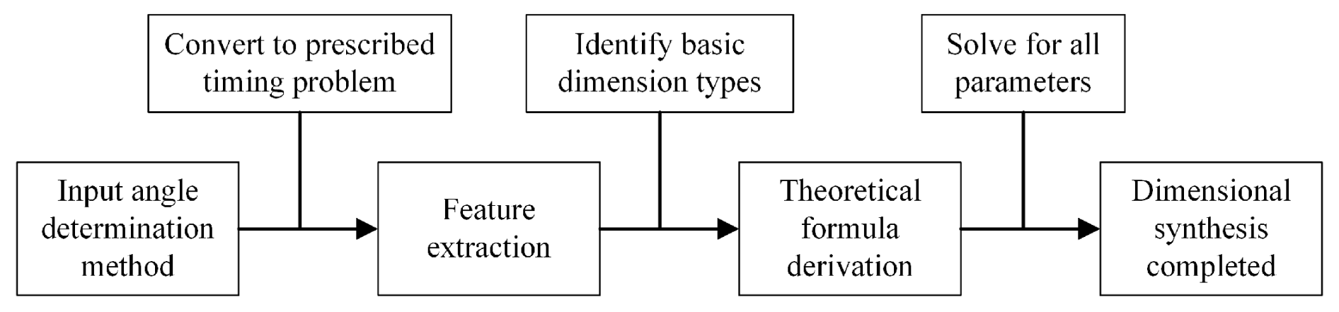
For the dimensional synthesis of spatial RRSC rigid-body guidance mechanisms without prescribed timing, the large number of dimensional parameters makes it highly challenging to adopt a full-parameter synchronous design approach, and it is difficult to obtain a solution. As the numerical atlas method is well-suited for dimensional synthesis with prescribed timing, our idea is to first provide a timing supplement method for the mechanism, thereby transforming the unprescribed-timing dimensional synthesis problem into a prescribed-timing problem. Based on this, since previous research has revealed that the coupler angle of the mechanism is only related to its basic dimensional types (for the spatial RRSC mechanism, the basic dimensional types are a₁, a₂, a₃, a₄, S₁, S₂, α₁₂, and α₄₁), if we can extract the characteristics of the coupler angle of the desired mechanism from design requirements, we can easily obtain the basic dimensional parameters of the target mechanism. On this basis, using the parametric equation of the coupler point of the mechanism, we can derive formulas to calculate the remaining dimensional parameters, thus solving all of the dimensional parameters of the mechanism and achieving mechanism synthesis. The technical route is shown in Fig. 2.

2.2 Input angle determination method for spatial RRSC mechanisms in a standard installation position

Based on the motion law of the R–R two-link mechanism, we found that, after specific processing of the rigid-body guidance lines of the mechanism, the points P and Q on the guidance lines will have distinct characteristics. The processing is divided into two steps. The first step is to rotate the guidance lines clockwise around the z_d axis by the input angle (θ₁). After processing, the coordinates of the obtained points ⁿP^′ and ⁿQ^′ of the nth rigid-body guidance line can be expressed as follows:

$$\begin{array}{}\text{(27)}& {\displaystyle }\begin{array}{rl}& \left[\begin{array}{c}{x}_P{}^{\prime }{(}^n{\mathit{\theta }}_{\mathrm{1}})\\ y_P{}^{\prime }{(}^n{\mathit{\theta }}_{\mathrm{1}})\\ z_P{}^{\prime }{(}^n{\mathit{\theta }}_{\mathrm{1}})\end{array}\right]=R_{z_d}^{-{}_{}^n{\mathit{\theta }}_{\mathrm{1}}}\left[\begin{array}{c}{x}_P{(}^n{\mathit{\theta }}_{\mathrm{1}})\\ y_P{(}^n{\mathit{\theta }}_{\mathrm{1}})\\ z_P{(}^n{\mathit{\theta }}_{\mathrm{1}})\end{array}\right]\\ & =\left[\begin{array}{c}{r}_P\sin {\mathit{\alpha }}_{Pz}\cos \left({\mathit{\alpha }}_{Pxy}{-}^n{\mathit{\theta }}_{\mathrm{2}}\right)+a_{\mathrm{1}}\\ r_P\sin {\mathit{\alpha }}_{Pz}\cos {\mathit{\alpha }}_{\mathrm{12}}\sin \left({\mathit{\alpha }}_{Pxy}{-}^n{\mathit{\theta }}_{\mathrm{2}}\right)-(r_P\cos {\mathit{\alpha }}_{Pz}-S_{\mathrm{2}})\sin {\mathit{\alpha }}_{\mathrm{12}}\\ \left(r_P\cos {\mathit{\alpha }}_{Pz}-S_{\mathrm{2}}\right)\cos {\mathit{\alpha }}_{\mathrm{12}}+r_P\sin {\mathit{\alpha }}_{Pz}\sin \left({\mathit{\alpha }}_{Pxy}{-}^n{\mathit{\theta }}_{\mathrm{2}}\right)\sin {\mathit{\alpha }}_{\mathrm{12}}+S_{\mathrm{1}}\end{array}\right],\end{array}\text{(28)}& {\displaystyle }\begin{array}{rl}& \left[\begin{array}{c}{x}_Q{}^{\prime }{(}^n{\mathit{\theta }}_{\mathrm{1}})\\ y_Q{}^{\prime }{(}^n{\mathit{\theta }}_{\mathrm{1}})\\ z_Q{}^{\prime }{(}^n{\mathit{\theta }}_{\mathrm{1}})\end{array}\right]=R_{z_d}^{-{}_{}^n{\mathit{\theta }}_{\mathrm{1}}}\left[\begin{array}{c}{x}_Q{(}^n{\mathit{\theta }}_{\mathrm{1}})\\ y_Q{(}^n{\mathit{\theta }}_{\mathrm{1}})\\ z_Q{(}^n{\mathit{\theta }}_{\mathrm{1}})\end{array}\right]\\ & =\left[\begin{array}{c}{r}_Q\sin {\mathit{\alpha }}_{Qz}\cos \left({\mathit{\alpha }}_{Qxy}{-}^n{\mathit{\theta }}_{\mathrm{2}}\right)+a_{\mathrm{1}}\\ r_Q\sin {\mathit{\alpha }}_{Qz}\cos {\mathit{\alpha }}_{\mathrm{12}}\sin \left({\mathit{\alpha }}_{Qxy}{-}^n{\mathit{\theta }}_{\mathrm{2}}\right)-(r_Q\cos {\mathit{\alpha }}_{Qz}-S_{\mathrm{2}})\sin {\mathit{\alpha }}_{\mathrm{12}}\\ \left(r_Q\cos {\mathit{\alpha }}_{Qz}-S_{\mathrm{2}}\right)\cos {\mathit{\alpha }}_{\mathrm{12}}+r_Q\sin {\mathit{\alpha }}_{Qz}\sin \left({\mathit{\alpha }}_{Qxy}{-}^n{\mathit{\theta }}_{\mathrm{2}}\right)\sin {\mathit{\alpha }}_{\mathrm{12}}+S_{\mathrm{1}}\end{array}\right],\end{array}\end{array}$$

where $R_{z_d}^{{-}^n{\mathit{\theta }}_{\mathrm{1}}}$ is the rotation matrix and can be expressed as

$$\begin{array}{}\text{(29)}& R_{z_d}^{{}^n{\mathit{\theta }}_{\mathrm{1}}}=\left[\begin{array}{ccc}{\cos }^n{\mathit{\theta }}_{\mathrm{1}}& {\sin }^n{\mathit{\theta }}_{\mathrm{1}}& \mathrm{0}\\ -si{n}^n{\mathit{\theta }}_{\mathrm{1}}& {\cos }^n{\mathit{\theta }}_{\mathrm{1}}& \mathrm{0}\\ \mathrm{0}& \mathrm{0}& \mathrm{1}\end{array}\right].\end{array}$$

The second step is to rotate the rigid-body guidance lines obtained from the first step clockwise around the x_d axis by α₁₂ (the angle between the rotation axis of the input link and the rotation axis of the coupler link), and then the coordinates of obtained points ⁿP^′′ and ⁿQ^′′ of the nth rigid-body guidance line can be expressed as follows:

$$\begin{array}{}\text{(30)}& {\displaystyle }\begin{array}{rl}& \left[\begin{array}{c}{x}_P{}^{\prime \prime }{(}^n{\mathit{\theta }}_{\mathrm{1}})\\ y_P{}^{\prime \prime }{(}^n{\mathit{\theta }}_{\mathrm{1}})\\ z_P{}^{\prime \prime }{(}^n{\mathit{\theta }}_{\mathrm{1}})\end{array}\right]=R_{x_d}^{-{\mathit{\alpha }}_{\mathrm{12}}}\left[\begin{array}{c}{x}_P{}^{\prime }{(}^n{\mathit{\theta }}_{\mathrm{1}})\\ y_P{}^{\prime }{(}^n{\mathit{\theta }}_{\mathrm{1}})\\ z_P{}^{\prime }{(}^n{\mathit{\theta }}_{\mathrm{1}})\end{array}\right]\\ & =\left[\begin{array}{c}{r}_P\sin {\mathit{\alpha }}_{Pz}\cos \left({\mathit{\alpha }}_{Pxy}{-}^n{\mathit{\theta }}_{\mathrm{2}}\right)+a_{\mathrm{1}}\\ r_P\sin {\mathit{\alpha }}_{Pz}\sin \left({\mathit{\alpha }}_{Pxy}{-}^n{\mathit{\theta }}_{\mathrm{2}}\right)+S_{\mathrm{1}}\sin {\mathit{\alpha }}_{\mathrm{12}}\\ r_P\cos {\mathit{\alpha }}_{P_z}-S_{\mathrm{2}}+S_{\mathrm{1}}\cos {\mathit{\alpha }}_{\mathrm{12}}\end{array}\right],\end{array}\text{(31)}& {\displaystyle }\begin{array}{rl}& \left[\begin{array}{c}{x}_Q{}^{\prime \prime }{(}^n{\mathit{\theta }}_{\mathrm{1}})\\ y_Q{}^{\prime \prime }{(}^n{\mathit{\theta }}_{\mathrm{1}})\\ z_Q{}^{\prime \prime }{(}^n{\mathit{\theta }}_{\mathrm{1}})\end{array}\right]=R_{x_d}^{-{\mathit{\alpha }}_{\mathrm{12}}}\left[\begin{array}{c}{x}_Q{}^{\prime }{(}^n{\mathit{\theta }}_{\mathrm{1}})\\ y_Q{}^{\prime }{(}^n{\mathit{\theta }}_{\mathrm{1}})\\ z_Q{}^{\prime }{(}^n{\mathit{\theta }}_{\mathrm{1}})\end{array}\right]\\ & =\left[\begin{array}{c}{r}_Q\sin {\mathit{\alpha }}_{Qz}\cos \left({\mathit{\alpha }}_{Qxy}{-}^n{\mathit{\theta }}_{\mathrm{2}}\right)+a_{\mathrm{1}}\\ r_Q\sin {\mathit{\alpha }}_{Qz}\sin \left({\mathit{\alpha }}_{Qxy}{-}^n{\mathit{\theta }}_{\mathrm{2}}\right)+S_{\mathrm{1}}\sin {\mathit{\alpha }}_{\mathrm{12}}\\ r_Q\cos {\mathit{\alpha }}_{Q_z}-S_{\mathrm{2}}+S_{\mathrm{1}}\cos {\mathit{\alpha }}_{\mathrm{12}}\end{array}\right],\end{array}\end{array}$$

where $R_{x_d}^{-{\mathit{\alpha }}_{\mathrm{12}}}$ is the rotation matrix and can be expressed as

$$\begin{array}{}\text{(32)}& \begin{array}{rl}& R_{x_d}^{-{\mathit{\alpha }}_{\mathrm{12}}}=\left[\begin{array}{ccc}\mathrm{1}& \mathrm{0}& \mathrm{0}\\ \mathrm{0}& \cos {\mathit{\alpha }}_{\mathrm{12}}& \sin {\mathit{\alpha }}_{\mathrm{12}}\\ \mathrm{0}& -sin{\mathit{\alpha }}_{\mathrm{12}}& \cos {\mathit{\alpha }}_{\mathrm{12}}\end{array}\right]\\ & \left[\begin{array}{c}{r}_Q\sin {\mathit{\alpha }}_{Qz}\cos \left({\mathit{\alpha }}_{Qxy}{-}^n{\mathit{\theta }}_{\mathrm{2}}\right)+a_{\mathrm{1}}\\ r_Q\sin {\mathit{\alpha }}_{Qz}\cos {\mathit{\alpha }}_{\mathrm{12}}\sin \left({\mathit{\alpha }}_{Qxy}{-}^n{\mathit{\theta }}_{\mathrm{2}}\right)-(r_Q\cos {\mathit{\alpha }}_{Qz}-S_{\mathrm{2}})\sin {\mathit{\alpha }}_{\mathrm{12}}\\ \left(r_Q\cos {\mathit{\alpha }}_{Qz}-S_{\mathrm{2}}\right)\cos {\mathit{\alpha }}_{\mathrm{12}}+r_Q\sin {\mathit{\alpha }}_{Qz}\sin \left({\mathit{\alpha }}_{Qxy}{-}^n{\mathit{\theta }}_{\mathrm{2}}\right)\sin {\mathit{\alpha }}_{\mathrm{12}}+S_{\mathrm{1}}\end{array}\right].\end{array}\end{array}$$

Based on Eq. (30), the following can be obtained:

$$\begin{array}{}\text{(33)}& {\displaystyle }{x}_P{}^{\prime \prime }{(}^n{\mathit{\theta }}_{\mathrm{1}})-a_{\mathrm{1}}=r_P\sin {\mathit{\alpha }}_{Pz}\cos ({\mathit{\alpha }}_{Pxy}{-}^n{\mathit{\theta }}_{\mathrm{2}}),\text{(34)}& {\displaystyle }{y}_P{}^{\prime \prime }{(}^n{\mathit{\theta }}_{\mathrm{1}})-S_{\mathrm{1}}\sin {\mathit{\alpha }}_{\mathrm{12}}=r_P\sin {\mathit{\alpha }}_{Pz}\sin ({\mathit{\alpha }}_{Pxy}{-}^n{\mathit{\theta }}_{\mathrm{2}}).\end{array}$$

Combining Eqs. (33) and (34) yields

$$\begin{array}{}\text{(35)}& \begin{array}{rl}{\left[x_P{}^{\prime \prime }{(}^n{\mathit{\theta }}_{\mathrm{1}})-a_{\mathrm{1}}\right]}^{\mathrm{2}}& +{\left[y_P{}^{\prime \prime }{(}^n{\mathit{\theta }}_{\mathrm{1}})-S_{\mathrm{1}}\sin {\mathit{\alpha }}_{\mathrm{12}}\right]}^{\mathrm{2}}\\ & ={\left(r_P\sin {\mathit{\alpha }}_{Pz}\right)}^{\mathrm{2}}.\end{array}\end{array}$$

For a specific spatial RRSC mechanism, a₁, S₁, S₂, r_P, r_Q, α₁₂, α_Pxy, α_Qxy, α_Pz, and α_Qz are fixed values. So, in Eq. (35), the input angle ⁿθ₁ is the unique variable; the other parameters are all constant values. According to the standard equation of a circle, it is obvious that x_P^′′(ⁿθ₁) and y_P^′′(ⁿθ₁) are the coordinates of a point whose projection on the xOy plane falls on a circle. Based on Eq. (30), z_P^′′(ⁿθ₁) is a fixed value because all parameters in the expression of z_P^′′(ⁿθ₁) are constant values. From this, we can draw a conclusion that the projection of point ⁿP^′′ on the xOy plane is a circle, and the z coordinate is a fixed value. Therefore, point ⁿP^′′ is a point on this circle, with a centre at (a₁, S₁sin α₁₂, r_Pcos α_PzS₂+S₁cos α₁₂) and a radius of R_P=r_Psin α_Pz. Similarly, point ⁿQ^′′ is also a point on another circle, with a centre at (a₁, S₁sin α₁₂, r_Qcos α_QzS₂+S₁cos α₁₂) and a radius of R_Q=r_Qsin α_Qz. Figure 3 shows the circles.

Figure 3 The coupler points after the processing.

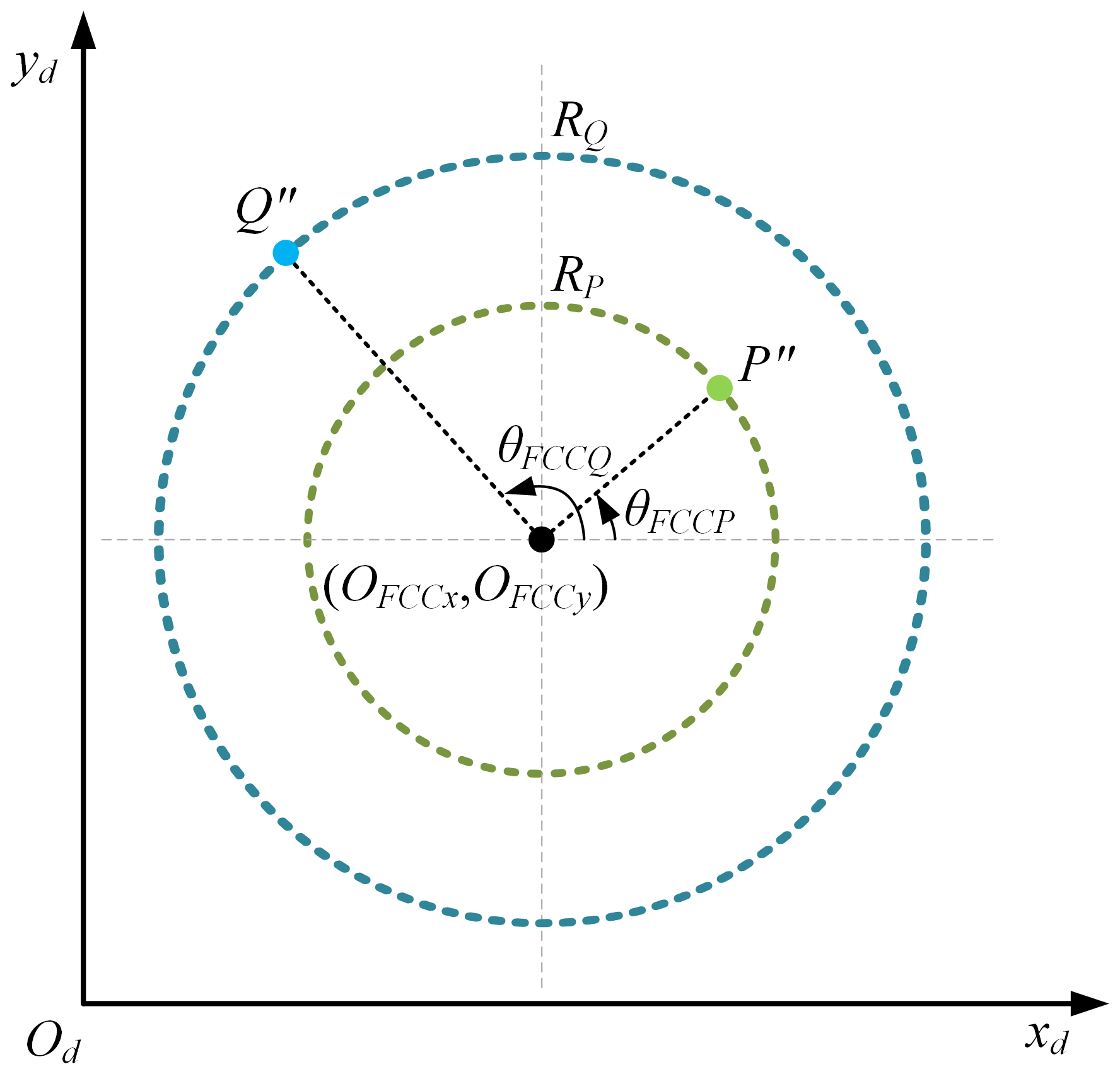
The circles are represented as ⊙P and ⊙Q. They are defined as feature coupler circles, abbreviated as FCC. The origin coordinates of ⊙P and ⊙Q are represented as $O_{P^{\prime \prime }}$ and $O_{Q^{\prime \prime }}$, respectively. The angle between the x_d axis and $O_{P^{\prime \prime }}^n{P}^{\prime \prime }$ is a_Pxy−ⁿθ₂; the angle between the xd axis and $O_{Q^{\prime \prime }}^n{Q}^{\prime \prime }$ is a_Qxy−ⁿθ₂. They are defined as feature central angles (expressed as ⁿθ_FCCP and ⁿθ_FCCQ). The points ⁿP^′′ and ⁿQ^′′ of the processed nth rigid-body guidance line are defined as feature coupler points. The direction of the processed rigid-body guidance line $P^{\prime \prime }{Q}^{\prime \prime }$ can be expressed as follows:

$$\begin{array}{}\text{(36)}& \begin{array}{rl}& \left[\begin{array}{c}{x}_Q{}^{\prime \prime }{(}^n{\mathit{\theta }}_{\mathrm{1}})\\ y_Q{}^{\prime \prime }{(}^n{\mathit{\theta }}_{\mathrm{1}})\\ z_Q{}^{\prime \prime }{(}^n{\mathit{\theta }}_{\mathrm{1}})\end{array}\right]\left[\begin{array}{c}{x}_P{}^{\prime \prime }{(}^n{\mathit{\theta }}_{\mathrm{1}})\\ y_P{}^{\prime \prime }{(}^n{\mathit{\theta }}_{\mathrm{1}})\\ z_P{}^{\prime \prime }{(}^n{\mathit{\theta }}_{\mathrm{1}})\end{array}\right]\\ & =\left[\begin{array}{c}{r}_Q\sin {\mathit{\alpha }}_{Qz}\cos \left({\mathit{\alpha }}_{Qxy}{-}^n{\mathit{\theta }}_{\mathrm{2}}\right)-r_P\sin {\mathit{\alpha }}_{Pz}\cos \left({\mathit{\alpha }}_{Pxy}{-}^n{\mathit{\theta }}_{\mathrm{2}}\right)\\ r_Q\sin {\mathit{\alpha }}_{Qz}\sin \left({\mathit{\alpha }}_{Qxy}{-}^n{\mathit{\theta }}_{\mathrm{2}}\right)-r_P\sin {\mathit{\alpha }}_{Pz}\sin \left({\mathit{\alpha }}_{Pxy}{-}^n{\mathit{\theta }}_{\mathrm{2}}\right)\\ r_Q\cos {\mathit{\alpha }}_{Qz}-r_P\cos {\mathit{\alpha }}_{Pz}\end{array}\right].\end{array}\end{array}$$

According to the first step of the processing, we can obtain

$$\begin{array}{}\text{(37)}& {\displaystyle }\begin{array}{rl}{y}_Q{}^{\prime }& {(}^n{\mathit{\theta }}_{\mathrm{1}})-y_P{}^{\prime }{(}^n{\mathit{\theta }}_{\mathrm{1}})=\left[y_Q{(}^n{\mathit{\theta }}_{\mathrm{1}}\right)-y_P{(}^n{\mathit{\theta }}_{\mathrm{1}}\left)\right]{\cos }^n{\mathit{\theta }}_{\mathrm{1}}\\ & -\left[x_Q{(}^n{\mathit{\theta }}_{\mathrm{1}}\right)-x_P{(}^n{\mathit{\theta }}_{\mathrm{1}}\left)\right]{\sin }^n{\mathit{\theta }}_{\mathrm{1}},\end{array}\text{(38)}& {\displaystyle }\begin{array}{rl}{z}_Q{}^{\prime }& {(}^n{\mathit{\theta }}_{\mathrm{1}})-z_P{}^{\prime }{(}^n{\mathit{\theta }}_{\mathrm{1}})=z_Q{(}^n{\mathit{\theta }}_{\mathrm{1}})-z_P{(}^n{\mathit{\theta }}_{\mathrm{1}})\\ & =\left(r_Q\cos {\mathit{\alpha }}_{Qz}{r}_P\cos {\mathit{\alpha }}_{Pz}\right)\cos {\mathit{\alpha }}_{\mathrm{12}}\\ & +[r_Q\sin {\mathit{\alpha }}_{Qz}\sin \left({\mathit{\alpha }}_{Qxy}-{\mathit{\theta }}_{\mathrm{2}}\right)r_P\sin {\mathit{\alpha }}_{Pz}\\ & \cos {\mathit{\alpha }}_{\mathrm{12}}\sin \left({\mathit{\alpha }}_{Pxy}-{\mathit{\theta }}_{\mathrm{2}}\right)]\sin {\mathit{\alpha }}_{\mathrm{12}}.\end{array}\end{array}$$

Substituting Eqs. (1) and (2) into Eq. (37) yields

$$\begin{array}{}\text{(39)}& \begin{array}{rl}{y}_Q{}^{\prime }& {(}^n{\mathit{\theta }}_{\mathrm{1}})-y_P{}^{\prime }{(}^n{\mathit{\theta }}_{\mathrm{1}})=[r_Q\sin {\mathit{\alpha }}_{Qz}\sin \left({\mathit{\alpha }}_{Qxy}{-}^n{\mathit{\theta }}_{\mathrm{2}}\right)r_P\\ & \sin {\mathit{\alpha }}_{Pz}\cos {\mathit{\alpha }}_{\mathrm{12}}\sin \left({\mathit{\alpha }}_{Pxy}{-}^n{\mathit{\theta }}_{\mathrm{2}}\right)]\cos {\mathit{\alpha }}_{\mathrm{12}}\\ & \left(r_Q\cos {\mathit{\alpha }}_{Qz}-r_P\cos {\mathit{\alpha }}_{Pz}\right)\sin {\mathit{\alpha }}_{\mathrm{12}}.\end{array}\end{array}$$

Substituting Eqs. (36) and (38) into Eq. (39) yields

$$\begin{array}{}\text{(40)}& \begin{array}{rl}& y_Q{}^{\prime }{(}^n{\mathit{\theta }}_{\mathrm{1}})-y_P{}^{\prime }{(}^n{\mathit{\theta }}_{\mathrm{1}})=\\ & {\displaystyle \frac{\left[z_Q{(}^n{\mathit{\theta }}_{\mathrm{1}})-z_P{(}^n{\mathit{\theta }}_{\mathrm{1}})\right]\cos {\mathit{\alpha }}_{\mathrm{12}}-\left[z_Q{}^{\prime \prime }{(}^{\mathrm{1}}{\mathit{\theta }}_{\mathrm{1}})-z_P{}^{\prime \prime }{(}^{\mathrm{1}}{\mathit{\theta }}_{\mathrm{1}})\right]}{\sin {\mathit{\alpha }}_{\mathrm{12}}}}.\end{array}\end{array}$$

Substituting Eq. (40) into Eq. (37), the input angle of the nth rigid-body guidance line can be obtained:

$$\begin{array}{}\text{(41)}& {}^n{\mathit{\theta }}_{\mathrm{1}}=\arcsin \left({\displaystyle \frac{b_{\mathrm{4}}}{\sqrt{b_{\mathrm{2}}^{\mathrm{2}}+b_{\mathrm{3}}^{\mathrm{2}}}}}\right)-\arctan \left({\displaystyle \frac{b_{\mathrm{2}}}{b_{\mathrm{3}}}}\right),\text{(42)}& {\displaystyle }{b}_{\mathrm{2}}=y_Q{(}^n{\mathit{\theta }}_{\mathrm{1}})-y_P{(}^n{\mathit{\theta }}_{\mathrm{1}}),\text{(43)}& {\displaystyle }{b}_{\mathrm{3}}=x_P{(}^n{\mathit{\theta }}_{\mathrm{1}}\left)x_Q{(}^n{\mathit{\theta }}_{\mathrm{1}}\right),\text{(44)}& {\displaystyle }{b}_{\mathrm{4}}=y_Q{}^{\prime }{(}^n{\mathit{\theta }}_{\mathrm{1}})-y_P{}^{\prime }{(}^n{\mathit{\theta }}_{\mathrm{1}}),\end{array}$$

where x_P(ⁿθ₁), y_P(ⁿθ₁), and z_P(ⁿθ₁) are the coordinates of point P on the nth rigid-body guidance line; x_Q(ⁿθ₁), y_Q(ⁿθ₁), and z_Q(ⁿθ₁) are the coordinates of point Q on the nth rigid-body guidance line; and z_P^′′(¹θ₁) and z_Q^′′(¹θ₁) are the z coordinate of the first feature coupler point ¹P^′′ and ¹Q^′′. Because ¹P^′′ and ¹Q^′′ are obtained by rotating the guidance lines clockwise around the z_d axis by the initial input angle (¹θ₁) and then rotating the rigid-body guidance lines obtained from the first step anticlockwise around thex_g axis by α₁₂, if we know the initial input angle and α₁₂, all of the input angles corresponding to the rigid-body guidance lines can be determined.

According to Eqs. (33) and (34), the central angle ⁿθ_FCCP of the corresponding feature coupler point ⁿP^′′ is related to a_Pxy and ⁿθ₂, and the feature central angle ⁿ⁺¹θ_FCCP of the feature coupler point ${}^{n+\mathrm{1}}{P}^{\prime \prime }$ is related to a_Pxy and ⁿ⁺¹θ₂. So, if we can determine the feature central angles ⁿ⁺¹θ_FCCP and ⁿθ_FCCP of the feature coupler points ${}^{n+\mathrm{1}}{P}^{\prime \prime }$ and ⁿP^′′, the difference between the coupler angles of two corresponding adjacent rigid-body guidance lines (${}^{n+\mathrm{1}}{\mathit{\theta }}_{\mathrm{2}}{-}^n{\mathit{\theta }}_{\mathrm{2}}$) can be determined. Furthermore, the basic dimensional types of the desired mechanism can be obtained because the coupler angles are only related to the basic dimensional types, which are the most basic dimensions that constitute a linkage mechanism (for the spatial RRSC mechanism, the basic dimensional types are a₁, a₂, a₃, a₄, S₁, S₂, α₁₂, and α₄₁). In other words, the feature central angles can be used to decouple the basic dimensional types from the geometric parameters. To reduce the dimensionality of the design variables, the theoretical calculation formula for the difference of the coupler angle of the mechanism is derived. First, according to Eq. (36), the following equations can be obtained:

$$\begin{array}{}\text{(45)}& {\displaystyle }\begin{array}{rl}{x}_Q{}^{\prime \prime }& {(}^n{\mathit{\theta }}_{\mathrm{1}})-x_P{}^{\prime \prime }{(}^n{\mathit{\theta }}_{\mathrm{1}})=\left(r_Q\sin {\mathit{\alpha }}_{Qz}\cos {\mathit{\alpha }}_{Qxy}-r_P\sin {\mathit{\alpha }}_{Pz}\right.\\ & \left.\cos {\mathit{\alpha }}_{Pxy}\right){\cos }^n{\mathit{\theta }}_{\mathrm{2}}+(r_Q\sin {\mathit{\alpha }}_{Qz}\\ & \sin {\mathit{\alpha }}_{Qxy}-r_P\sin {\mathit{\alpha }}_{Pz}\sin {\mathit{\alpha }}_{Pxy}){\sin }^n{\mathit{\theta }}_{\mathrm{2}},\end{array}\text{(46)}& {\displaystyle }\begin{array}{rl}{y}_Q{}^{\prime \prime }& {(}^n{\mathit{\theta }}_{\mathrm{1}})-y_P{}^{\prime \prime }{(}^n{\mathit{\theta }}_{\mathrm{1}})=\left(r_Q\sin {\mathit{\alpha }}_{Qz}\sin {\mathit{\alpha }}_{Qxy}-r_P\sin {\mathit{\alpha }}_{Pz}\right.\\ & \left.\sin {\mathit{\alpha }}_{Pxy}\right){\cos }^n{\mathit{\theta }}_{\mathrm{2}}(r_Q\sin {\mathit{\alpha }}_{Qz}\cos {\mathit{\alpha }}_{Qxy}-r_P\sin {\mathit{\alpha }}_{Pz}\\ & \cos {\mathit{\alpha }}_{Pxy}){\sin }^n{\mathit{\theta }}_{\mathrm{2}}.\end{array}\end{array}$$

Let $r_Q\sin a_{Qz}\cos a_{Qxy}-r_P\sin a_{Pz}\cos a_{Pxy}=k\cos \mathit{\tau }$ and $r_Q\sin a_{Qz}\sin a_{Qxy}-r_P\sin a_{Pz}\sin a_{Pxy}=k\sin \mathit{\tau }$; thus, Eqs. (45) and (46) can be expressed as follows:

$$\begin{array}{}\text{(47)}& {\displaystyle }{x}_Q{}^{\prime \prime }{(}^n{\mathit{\theta }}_{\mathrm{1}})-x_P{}^{\prime \prime }{(}^n{\mathit{\theta }}_{\mathrm{1}})=k\cos \mathit{\tau }{\cos }^n{\mathit{\theta }}_{\mathrm{2}}+k\sin \mathit{\tau }{\sin }^n{\mathit{\theta }}_{\mathrm{2}},\text{(48)}& {\displaystyle }{y}_Q{}^{\prime \prime }{(}^n{\mathit{\theta }}_{\mathrm{1}})-y_P{}^{\prime \prime }{(}^n{\mathit{\theta }}_{\mathrm{1}})=k\sin \mathit{\tau }{\cos }^n{\mathit{\theta }}_{\mathrm{2}}k\cos \mathit{\tau }{\sin }^n{\mathit{\theta }}_{\mathrm{2}}.\end{array}$$

It is important to note that k and τ are intermediate variables with no direct physical meaning, serving purely as mathematical constructs to streamline the workflow. Arranging Eqs. (47) and (48) yields

$$\begin{array}{}\text{(49)}& {\displaystyle }{x}_Q{}^{\prime \prime }{(}^n{\mathit{\theta }}_{\mathrm{1}})-x_P{}^{\prime \prime }{(}^n{\mathit{\theta }}_{\mathrm{1}})=k\cos \left(\mathit{\tau }{-}^n{\mathit{\theta }}_{\mathrm{2}}\right),\text{(50)}& {\displaystyle }{y}_Q{}^{\prime \prime }{(}^n{\mathit{\theta }}_{\mathrm{1}})-y_P{}^{\prime \prime }{(}^n{\mathit{\theta }}_{\mathrm{1}})=k\sin \left(\mathit{\tau }{-}^n{\mathit{\theta }}_{\mathrm{2}}\right).\end{array}$$

Based on Eqs. (49) and (50), we have

$$\begin{array}{}\text{(51)}& {\displaystyle \frac{y_Q{}^{\prime \prime }{(}^n{\mathit{\theta }}_{\mathrm{1}})-y_P{}^{\prime \prime }{(}^n{\mathit{\theta }}_{\mathrm{1}})}{x_Q{}^{\prime \prime }{(}^n{\mathit{\theta }}_{\mathrm{1}})-x_P{}^{\prime \prime }{(}^n{\mathit{\theta }}_{\mathrm{1}})}}={\displaystyle \frac{k\sin \left(\mathit{\tau }{-}^n{\mathit{\theta }}_{\mathrm{2}}\right)}{k\cos \left(\mathit{\tau }{-}^n{\mathit{\theta }}_{\mathrm{2}}\right)}}=\tan \left(\mathit{\tau }{-}^n{\mathit{\theta }}_{\mathrm{2}}\right).\end{array}$$

The following can be obtained according to Eq. (51):

$$\begin{array}{}\text{(52)}& \arctan \left[{\displaystyle \frac{y_Q{}^{\prime \prime }{(}^n{\mathit{\theta }}_{\mathrm{1}})-y_P{}^{\prime \prime }{(}^n{\mathit{\theta }}_{\mathrm{1}})}{x_Q{}^{\prime \prime }{(}^n{\mathit{\theta }}_{\mathrm{1}})-x_P{}^{\prime \prime }{(}^n{\mathit{\theta }}_{\mathrm{1}})}}\right]={\mathit{\tau }}^n{\mathit{\theta }}_{\mathrm{2}}.\end{array}$$

Identically obtained is

$$\begin{array}{}\text{(53)}& \arctan \left[{\displaystyle \frac{y_Q{}^{\prime \prime }{(}^{n+\mathrm{1}}{\mathit{\theta }}_{\mathrm{1}})-y_P{}^{\prime \prime }{(}^{n+\mathrm{1}}{\mathit{\theta }}_{\mathrm{1}})}{x_Q{}^{\prime \prime }{(}^{n+\mathrm{1}}{\mathit{\theta }}_{\mathrm{1}})-x_P{}^{\prime \prime }{(}^{n+\mathrm{1}}{\mathit{\theta }}_{\mathrm{1}})}}\right]={\mathit{\tau }}^{n+\mathrm{1}}{\mathit{\theta }}_{\mathrm{2}}.\end{array}$$

According to Eqs. (52) and (53), the difference of the coupler angle can be expressed as follows:

$$\begin{array}{}\text{(54)}& \begin{array}{rl}{}^{n+\mathrm{1}}{\mathit{\theta }}_{\mathrm{2}}^n{\mathit{\theta }}_{\mathrm{2}}& =\arctan \left[{\displaystyle \frac{y_Q{}^{\prime \prime }{(}^n{\mathit{\theta }}_{\mathrm{1}})-y_P{}^{\prime \prime }{(}^n{\mathit{\theta }}_{\mathrm{1}})}{x_Q{}^{\prime \prime }{(}^n{\mathit{\theta }}_{\mathrm{1}})-x_P{}^{\prime \prime }{(}^n{\mathit{\theta }}_{\mathrm{1}})}}\right]\\ & -\arctan \left[{\displaystyle \frac{y_Q{}^{\prime \prime }{(}^{n+\mathrm{1}}{\mathit{\theta }}_{\mathrm{1}})-y_P{}^{\prime \prime }{(}^{n+\mathrm{1}}{\mathit{\theta }}_{\mathrm{1}})}{x_Q{}^{\prime \prime }{(}^{n+\mathrm{1}}{\mathit{\theta }}_{\mathrm{1}})-x_P{}^{\prime \prime }{(}^{n+\mathrm{1}}{\mathit{\theta }}_{\mathrm{1}})}}\right].\end{array}\end{array}$$

The above method of calculating the difference of the coupler angle provides a way to determine the basic dimensional types of the target mechanism by using the coordinates of the ⁿP^′′ and ⁿQ^′′ points of the preprocessed rigid-body guidance line.

2.3 Case verification

In this section, an example is presented to validate the proposed method. Firstly, we randomly give a set of geometric parameters of the mechanism and generate a spatial RRSC mechanism based on these parameters. Then, we sample the rigid-body guidance lines. Finally, we solve the input angles and the difference between the coupler angles of the mechanism according to the sampling information. If the solved values of the input angles and the difference between coupler angles are consistent with the actual values, this proves the validity of our method. The lengths of the links of the spatial RRSC mechanism are given as follows: a₁=80, a₂=200, a₃=170, a₄=140, S₁=270, and S₂=140. The angle between the rotation axes of the input link and coupler link is α₁₂=35°; the angle between the rotation axes of the driven link and the input link is α₄₁=16°. The positional parameters of the coupler points P and Q on the rigid-body guidance line are as follows: r_P=62, α_Pxy=36°, α_Pz=72°, r_Q=87, α_Qxy=55°, and α_Qz=93°. Nine rigid-body guidance lines are generated by the mechanism, and the coordinates of the P and Q points of the sampled rigid-body guidance lines are listed in Table 1. The corresponding input angles and coupler angles of the sampled rigid-body guidance lines are listed in Table 1. Now, using the coordinates of points P and Q of the rigid-body guidance line, the initial input angle of the mechanism (¹θ₁), and the angle between the rotation axis of the input link and the rotation axis of the coupler link (α₁₂), we will inversely determine the input angles and the difference between coupler angles.

Table 1 The values.

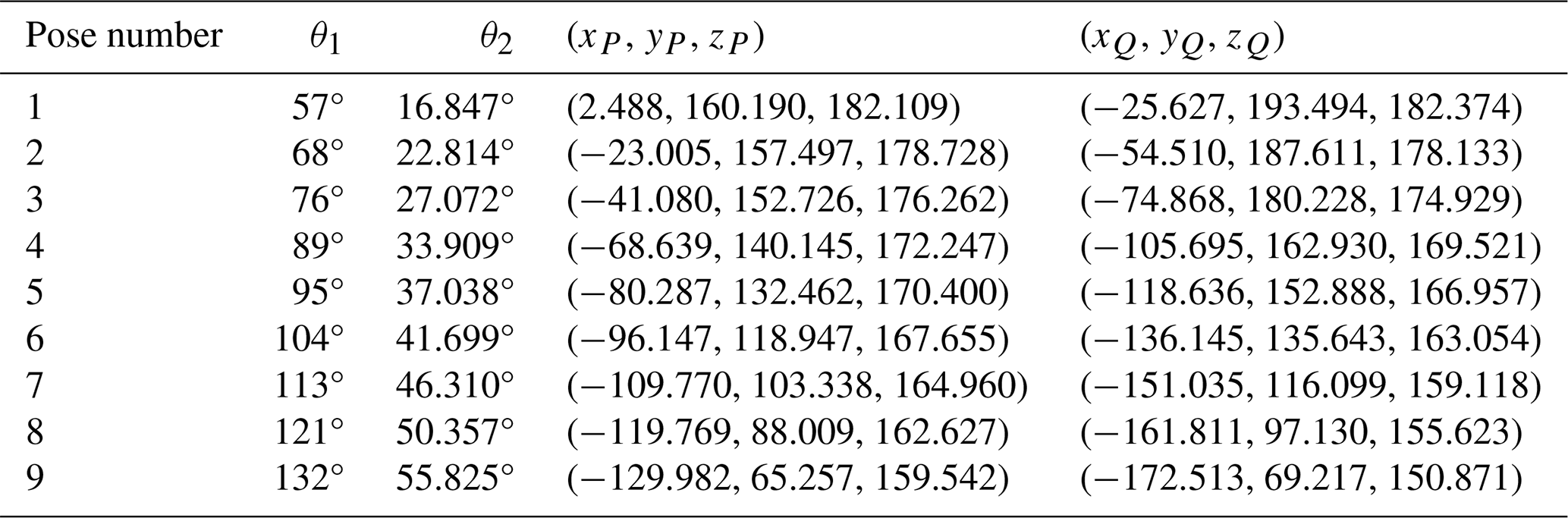
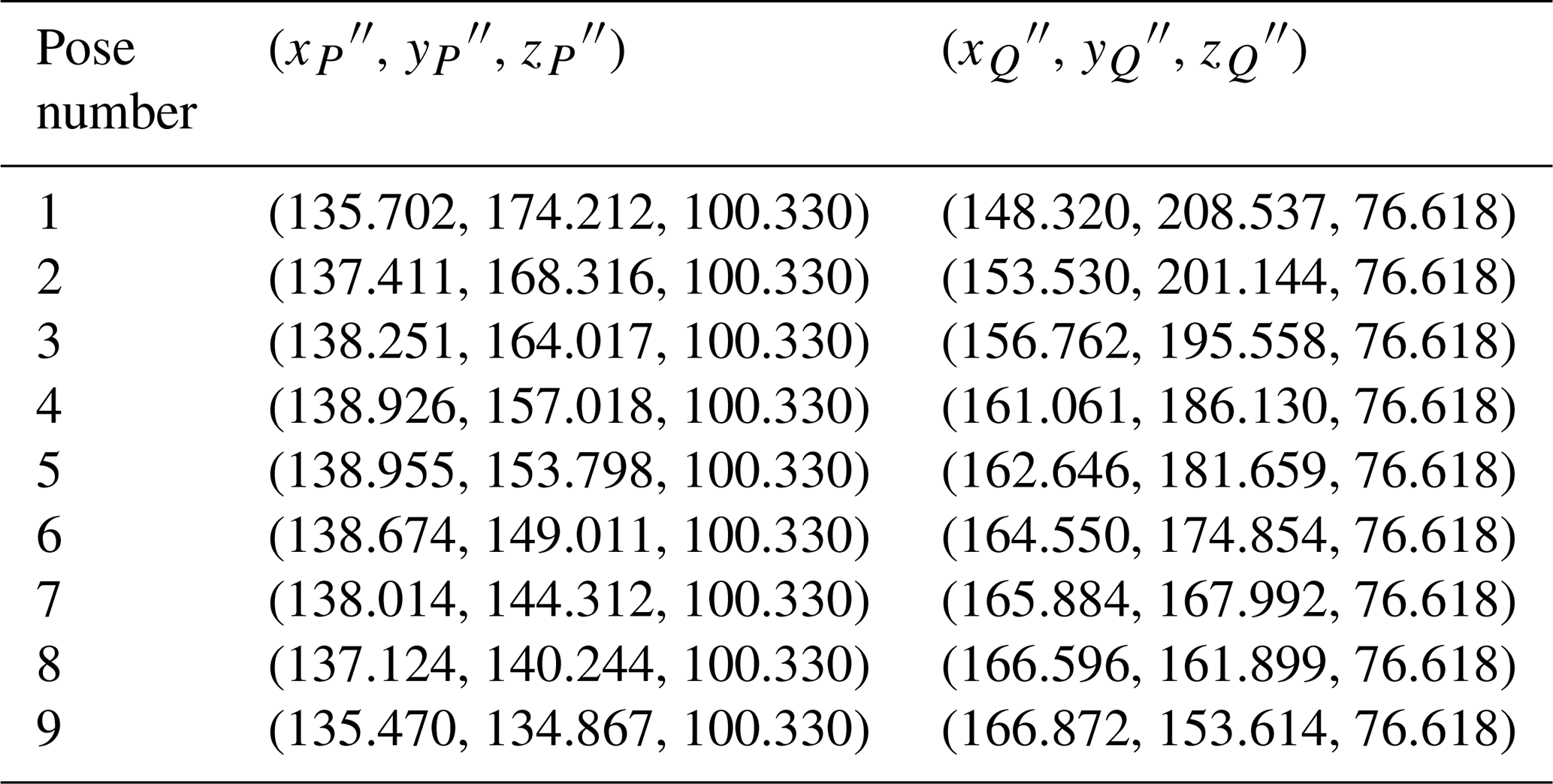
To determine the input angles, we need to know not only the coordinates of points P and Q of the rigid-body guidance line and the angle between the rotation axes of the input link and coupler link but also the first feature coupler point. To determine the first feature coupler point, we need to know the corresponding input angle of the mechanism at that point, which is the initial input angle of the mechanism. That is to say, the parameters we need include (x_P, y_P, z_P), (x_Q, y_Q, z_Q), α₁₂, and ¹θ₁. First, we calculate the y-axis and z-axis coordinates of the points P and Q on the first sampled guidance line after the first processing step. The first processing step is to rotate the ¹P and ¹Q clockwise around the z axis by the initial input angle (¹θ₁). The initial input angle is 57°, and the coordinates of (x_P(¹θ₁), y_P(¹θ₁), z_P(¹θ₁)) and (x_Q(¹θ₁), y_Q(¹θ₁), z_Q(¹θ₁)) are (2.488, 160.190, 182.109) and (−25.627, 193.494, 182.374). After processing, the coordinates of obtained points ¹P^′ and ¹Q^′ of the first rigid-body guidance line can be obtained; these are listed in Table 2.

The second step is to rotate the points ¹P^′ and ¹Q^′ clockwise around the x axis by α₁₂. The angle between the rotation axes of the input link and coupler link is 35°. Then the coordinates of the obtained points ¹P^′′ and ¹Q^′′ can be obtained; these are listed in Table 2.

Finally, the value of the rigid-body guidance line in the z-axis direction after the two-step processing is

$$z_Q{}^{\prime \prime }{(}^{\mathrm{1}}{\mathit{\theta }}_{\mathrm{1}})-z_P{}^{\prime \prime }{(}^{\mathrm{1}}{\mathit{\theta }}_{\mathrm{1}})=\mathrm{23.712}.$$

Table 2 The calculated values.

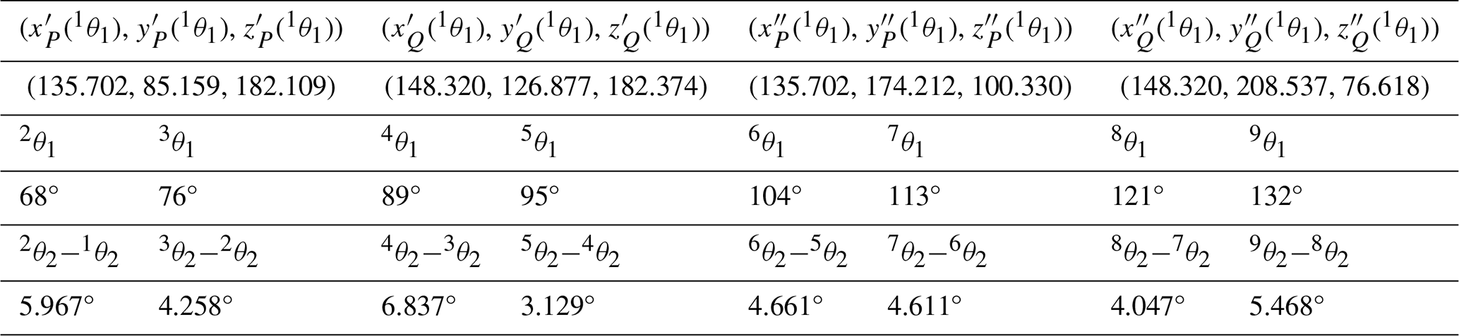
Substituting the value of $z_Q{}^{\prime \prime }{(}^{\mathrm{1}}{\mathit{\theta }}_{\mathrm{1}})-z_P{}^{\prime \prime }{(}^{\mathrm{1}}{\mathit{\theta }}_{\mathrm{1}})$, the coordinates of the points P and Q, and α₁₂ into Eq. (40), the values of each rigid-body guidance line in the y-axis direction after the first processing step can be obtained. Then, based on Eq. (41), the input angle corresponding to each rigid-body guidance line can be obtained; these are listed in Table 2.

Comparing the calculated input angles with the actual input angles of the mechanism (listed in Table 1), they have the same values, thus verifying the validity of the proposed input angle determination method. Since the input angles are obtained, the difference in terms of coupler angles can be calculated. Based on input angles and α₁₂, the feature coupler points can be obtained, and the coordinates are listed in Table 3. Substituting the coordinates of feature coupler point into Eq. (54), the difference in terms of coupler angle can be obtained; these are listed in Table 2. Comparing the calculated difference in coupler angles with the actual difference (the actual coupler angles are listed in Table 4), they have the same values, thus also verifying the validity of the proposed difference in terms of the coupler angle calculation method.

Table 3 The coordinates of feature coupler points.

Table 4 The difference in terms of coupler angles.

3 Dimensional synthesis methods for spatial RRSC rigid-body guidance mechanisms

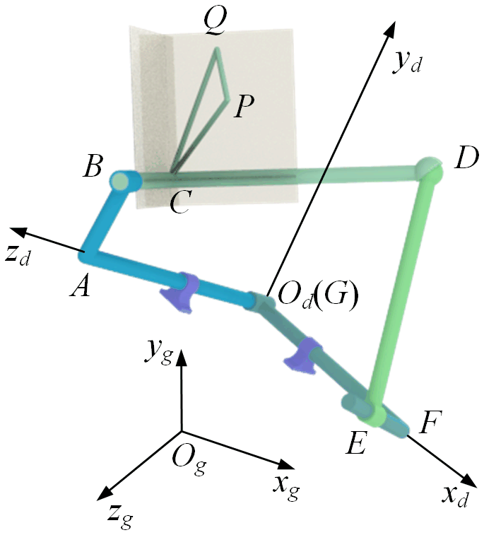
3.1 Input angle determination method for offset installation position spatial RRSC rigid-body guidance mechanism

In Sect. 2.2, an input angle determination method is proposed. However, the method is only suitable for the desired mechanism in a standard installation position. So, we need to extend the proposed method above to a spatial RRSC mechanism in a general installation position. Before that, we first discuss the mechanism in a specific installation position. We translate the frame of a standard installation mechanism along the x, y, and z axes by O_x, O_y, and O_z, respectively, to obtain a spatial RRSC mechanism in an offset installation position, as shown in Fig. 4. Based on Eqs. (1) and (2), the points ⁿP and ⁿQ of the nth rigid-body guidance line can be expressed as follows:

$$\begin{array}{}\text{(55)}& {\displaystyle }\begin{array}{rl}& \left[\begin{array}{c}{x}_P{(}^n{\mathit{\theta }}_{\mathrm{1}})\\ y_P{(}^n{\mathit{\theta }}_{\mathrm{1}})\\ z_P{(}^n{\mathit{\theta }}_{\mathrm{1}})\end{array}\right]\\ & =\left[\begin{array}{c}\left[r_P\sin {\mathit{\alpha }}_{Pz}\cos ({\mathit{\alpha }}_{Pxy}-{\mathit{\theta }}_{\mathrm{2}})+a_{\mathrm{1}}\right]\cos {\mathit{\theta }}_{\mathrm{1}}+\left[\left(r_P\cos {\mathit{\alpha }}_{Pz}-S_{\mathrm{2}}\right)\sin {\mathit{\alpha }}_{\mathrm{12}}-\left.r_P\sin {\mathit{\alpha }}_{Pz}\cos {\mathit{\alpha }}_{\mathrm{12}}\sin ({\mathit{\alpha }}_{Pxy}-{\mathit{\theta }}_{\mathrm{2}})\right]\sin {\mathit{\theta }}_{\mathrm{1}}+O_x\right.\\ \left[r_P\sin {\mathit{\alpha }}_{Pz}\cos ({\mathit{\alpha }}_{Pxy}-{\mathit{\theta }}_{\mathrm{2}})+a_{\mathrm{1}}\right]\cos {\mathit{\theta }}_{\mathrm{1}}-\left[\left(r_P\cos {\mathit{\alpha }}_{Pz}-S_{\mathrm{2}}\right)\sin {\mathit{\alpha }}_{\mathrm{12}}-\left.r_P\sin {\mathit{\alpha }}_{Pz}\cos {\mathit{\alpha }}_{\mathrm{12}}\sin ({\mathit{\alpha }}_{Pxy}-{\mathit{\theta }}_{\mathrm{2}})\right]\sin {\mathit{\theta }}_{\mathrm{1}}+O_y\right.\\ \left(r_P\cos {\mathit{\alpha }}_{Pz}-S_{\mathrm{2}}\right)\cos {\mathit{\alpha }}_{\mathrm{12}}+r_P\sin {\mathit{\alpha }}_{Pz}\sin \left({\mathit{\alpha }}_{Pxy}-{\mathit{\theta }}_{\mathrm{2}}\right)\sin {\mathit{\alpha }}_{\mathrm{12}}+S_{\mathrm{1}}+O_z\end{array}\right],\end{array}\text{(56)}& {\displaystyle }\begin{array}{rl}& \left[\begin{array}{c}{x}_Q{(}^n{\mathit{\theta }}_{\mathrm{1}})\\ y_Q{(}^n{\mathit{\theta }}_{\mathrm{1}})\\ z_Q{(}^n{\mathit{\theta }}_{\mathrm{1}})\end{array}\right]\\ & =\left[\begin{array}{c}\left[r_Q\sin {\mathit{\alpha }}_{Qz}\cos ({\mathit{\alpha }}_{Qxy}-{\mathit{\theta }}_{\mathrm{2}})+a_{\mathrm{1}}\right]\cos {\mathit{\theta }}_{\mathrm{1}}+\left[\left(r_Q\cos {\mathit{\alpha }}_{Qz}-S_{\mathrm{2}}\right)\sin {\mathit{\alpha }}_{\mathrm{12}}-\right.\left.r_Q\sin {\mathit{\alpha }}_{Qz}\cos {\mathit{\alpha }}_{\mathrm{12}}\sin ({\mathit{\alpha }}_{Qxy}-{\mathit{\theta }}_{\mathrm{2}})\right]\sin {\mathit{\theta }}_{\mathrm{1}}+O_x\\ \left[r_Q\sin {\mathit{\alpha }}_{Qz}\cos ({\mathit{\alpha }}_{Qxy}-{\mathit{\theta }}_{\mathrm{2}})+a_{\mathrm{1}}\right]\cos {\mathit{\theta }}_{\mathrm{1}}-\left[\left(r_Q\cos {\mathit{\alpha }}_{Qz}-S_{\mathrm{2}}\right)\sin {\mathit{\alpha }}_{\mathrm{12}}-\right.\left.r_Q\sin {\mathit{\alpha }}_{Qz}\cos {\mathit{\alpha }}_{\mathrm{12}}\sin ({\mathit{\alpha }}_{Qxy}-{\mathit{\theta }}_{\mathrm{2}})\right]\sin {\mathit{\theta }}_{\mathrm{1}}+O_y\\ \left(r_Q\cos {\mathit{\alpha }}_{Qz}-S_{\mathrm{2}}\right)\cos {\mathit{\alpha }}_{\mathrm{12}}+r_Q\sin {\mathit{\alpha }}_{Qz}\sin \left({\mathit{\alpha }}_{Qxy}-{\mathit{\theta }}_{\mathrm{2}}\right)\sin {\mathit{\alpha }}_{\mathrm{12}}+S_{\mathrm{1}}+O_z\end{array}\right].\end{array}\end{array}$$

According to Eqs. (55) and (56), it can be seen that the rigid-body guidance line of the spatial RRSC mechanism in the offset installation position is affected by the installation position parameters (O_x, O_y, and O_z). So, it is difficult to directly use the method proposed in Sect. 2.2 to obtain the input angles of the desired mechanism. In order to eliminate this influence, the direction vector of the rigid-body guidance line is used to describe the feature information of it. The projection of the direction vector on three coordinate axes can be expressed as follows:

$$\begin{array}{}\text{(57)}& \left[\begin{array}{c}{x}_Q^{}{(}^n{\mathit{\theta }}_{\mathrm{1}})\\ y_Q^{}{(}^n{\mathit{\theta }}_{\mathrm{1}})\\ z_Q^{}{(}^n{\mathit{\theta }}_{\mathrm{1}})\end{array}\right]\left[\begin{array}{c}{x}_P^{}{(}^n{\mathit{\theta }}_{\mathrm{1}})\\ y_P^{}{(}^n{\mathit{\theta }}_{\mathrm{1}})\\ z_P^{}{(}^n{\mathit{\theta }}_{\mathrm{1}})\end{array}\right]=\left[\begin{array}{c}{c}_{\mathrm{2}}\cos {\mathit{\theta }}_{\mathrm{1}}+c_{\mathrm{3}}\sin {\mathit{\theta }}_{\mathrm{1}}\\ c_{\mathrm{2}}\sin {\mathit{\theta }}_{\mathrm{1}}+c_{\mathrm{3}}\cos {\mathit{\theta }}_{\mathrm{1}}\\ c_{\mathrm{4}}\end{array}\right],\end{array}$$

where

$$\begin{array}{}\text{(58)}& {\displaystyle }{c}_{\mathrm{2}}=r_Q\sin {\mathit{\alpha }}_{Qz}\cos \left({\mathit{\alpha }}_{Qxy}{\mathit{\theta }}_{\mathrm{2}}\right)-r_P\sin {\mathit{\alpha }}_{Pz}\cos \left({\mathit{\alpha }}_{Pxy}{\mathit{\theta }}_{\mathrm{2}}\right),\text{(59)}& {\displaystyle }\begin{array}{rl}{c}_{\mathrm{3}}& =\left[\right(r_Q\cos {\mathit{\alpha }}_{Qz}{S}_{\mathrm{2}}\left)\sin {\mathit{\alpha }}_{\mathrm{12}}{r}_Q\sin {\mathit{\alpha }}_{Qz}\cos {\mathit{\alpha }}_{\mathrm{12}}\sin \right({\mathit{\alpha }}_{Qxy}{\mathit{\theta }}_{\mathrm{2}})\\ & -\left(r_P\cos {\mathit{\alpha }}_{Pz}{S}_{\mathrm{2}}\right)\sin {\mathit{\alpha }}_{\mathrm{12}}+r_P\sin {\mathit{\alpha }}_{Pz}\cos {\mathit{\alpha }}_{\mathrm{12}}\\ & \sin \left({\mathit{\alpha }}_{Pxy}{\mathit{\theta }}_{\mathrm{2}}\right)],\end{array}\text{(60)}& {\displaystyle }\begin{array}{rl}{c}_{\mathrm{4}}& =r_Q\cos {\mathit{\alpha }}_{Qz}\cos {\mathit{\alpha }}_{\mathrm{12}}+r_Q\sin {\mathit{\alpha }}_{Qz}\sin \left({\mathit{\alpha }}_{Qxy}-{\mathit{\theta }}_{\mathrm{2}}\right)\\ & \sin {\mathit{\alpha }}_{\mathrm{12}}{r}_P\cos {\mathit{\alpha }}_{Pz}\cos {\mathit{\alpha }}_{\mathrm{12}}+r_P\sin {\mathit{\alpha }}_{Pz}\sin \\ & \left({\mathit{\alpha }}_{Pxy}-{\mathit{\theta }}_{\mathrm{2}}\right)\sin {\mathit{\alpha }}_{\mathrm{12}}.\end{array}\end{array}$$

The direction vectors of the rigid-body guidance line are then processed using the processing method proposed in Sect. 2.2 as follows:

$$\begin{array}{}\text{(61)}& \begin{array}{rl}& \left[\begin{array}{c}{x}_Q{}^{\prime \prime }{(}^n{\mathit{\theta }}_{\mathrm{1}})\\ y_Q{}^{\prime \prime }{(}^n{\mathit{\theta }}_{\mathrm{1}})\\ z_Q{}^{\prime \prime }{(}^n{\mathit{\theta }}_{\mathrm{1}})\end{array}\right]\left[\begin{array}{c}{x}_P{}^{\prime \prime }{(}^n{\mathit{\theta }}_{\mathrm{1}})\\ y_P{}^{\prime \prime }{(}^n{\mathit{\theta }}_{\mathrm{1}})\\ z_P{}^{\prime \prime }{(}^n{\mathit{\theta }}_{\mathrm{1}})\end{array}\right]\\ & =\left[\begin{array}{c}{r}_Q\sin {\mathit{\alpha }}_{Qz}\cos \left({\mathit{\alpha }}_{Qxy}{-}^n{\mathit{\theta }}_{\mathrm{2}}\right)-r_P\sin {\mathit{\alpha }}_{Pz}\cos \left({\mathit{\alpha }}_{Pxy}{-}^n{\mathit{\theta }}_{\mathrm{2}}\right)\\ r_Q\sin {\mathit{\alpha }}_{Qz}\sin \left({\mathit{\alpha }}_{Qxy}{-}^n{\mathit{\theta }}_{\mathrm{2}}\right)-r_P\sin {\mathit{\alpha }}_{Pz}\sin \left({\mathit{\alpha }}_{Pxy}{-}^n{\mathit{\theta }}_{\mathrm{2}}\right)\\ r_Q\cos {\mathit{\alpha }}_{Qz}-r_P\cos {\mathit{\alpha }}_{Pz}\end{array}\right].\end{array}\end{array}$$

By comparing Eqs. (61) and (36), it can be found that the values are the same; therefore, it is straightforward to obtain the input angles:

$$\begin{array}{}\text{(62)}& {\mathit{\theta }}_{\mathrm{1}}=\arcsin \left({\displaystyle \frac{b_{\mathrm{7}}}{\sqrt{b_{\mathrm{5}}^{\mathrm{2}}+b_{\mathrm{6}}^{\mathrm{2}}}}}\right)-\arctan \left({\displaystyle \frac{b_{\mathrm{5}}}{b_{\mathrm{6}}}}\right),\end{array}$$

where

$$\begin{array}{}\text{(63)}& {\displaystyle }{b}_{\mathrm{5}}=y_Q{(}^n{\mathit{\theta }}_{\mathrm{1}})-y_P{(}^n{\mathit{\theta }}_{\mathrm{1}}),\text{(64)}& {\displaystyle }{b}_{\mathrm{6}}=x_P{(}^n{\mathit{\theta }}_{\mathrm{1}})-x_Q{(}^n{\mathit{\theta }}_{\mathrm{1}}),\text{(65)}& {\displaystyle }{b}_{\mathrm{7}}=y{{}^{\prime }}_Q{(}^n{\mathit{\theta }}_{\mathrm{1}})-y{{}^{\prime }}_P{(}^n{\mathit{\theta }}_{\mathrm{1}}).\end{array}$$

Similarly the difference of coupler angles can be obtained as follows:

$$\begin{array}{}\text{(66)}& \begin{array}{rl}{}^{n+\mathrm{1}}{\mathit{\theta }}_{\mathrm{2}}^n{\mathit{\theta }}_{\mathrm{2}}& =\arctan \left[{\displaystyle \frac{y_Q{}^{\prime \prime }{(}^n{\mathit{\theta }}_{\mathrm{1}})-y_P{}^{\prime \prime }{(}^n{\mathit{\theta }}_{\mathrm{1}})}{x_Q{}^{\prime \prime }{(}^n{\mathit{\theta }}_{\mathrm{1}})-x_P{}^{\prime \prime }{(}^n{\mathit{\theta }}_{\mathrm{1}})}}\right]\\ & -\arctan \left[{\displaystyle \frac{y_Q{}^{\prime \prime }{(}^{n+\mathrm{1}}{\mathit{\theta }}_{\mathrm{1}})-y_P{}^{\prime \prime }{(}^{n+\mathrm{1}}{\mathit{\theta }}_{\mathrm{1}})}{x_Q{}^{\prime \prime }{(}^{n+\mathrm{1}}{\mathit{\theta }}_{\mathrm{1}})-x_P{}^{\prime \prime }{(}^{n+\mathrm{1}}{\mathit{\theta }}_{\mathrm{1}})}}\right].\end{array}\end{array}$$

Figure 4 An RRSC rigid guidance mechanism in an offset installation position.

Figure 5 A spatial RRSC rigid-body guidance mechanism in a general installation position.

3.2 Input angle determination method for general-installation-position spatial RRSC rigid-body guide mechanism

Translating the frame of a spatial RRSC rigid-body guide mechanism in a standard installation position along the x_g axis, y_g axis, and z_g axis of the fixed coordinate system O_g-x_gy_gz_g by O_x, O_y, and O_z, respectively, and then rotating the frame of the translated mechanism around the x_g axis, y_g axis, and z_g axis by θ_x, θ_y, and  θ_z, respectively, allows us to obtain the spatial RRSC rigid-body guidance mechanism in a general installation position, as shown in Fig. 5. According to Eqs. (1) and (2), the ⁿP_g point coordinates (x_Pg, y_Pg, z_Pg) and ⁿQ_g point coordinates (x_Qg, y_Qg, z_Qg) of the nth (n=1, 2, …, N, where N is the total number of rigid-body guidance lines) rigid-body guidance line can be expressed in the global coordinate system O_g-x_gy_gz_g as follows:

$$\begin{array}{}\text{(67)}& {\displaystyle }\left[\begin{array}{c}{x}_{Pg}{(}^n{\mathit{\theta }}_{\mathrm{1}})\\ y_{Pg}{(}^n{\mathit{\theta }}_{\mathrm{1}})\\ z_{Pg}{(}^n{\mathit{\theta }}_{\mathrm{1}})\end{array}\right]=R_{z_g}^{{\mathit{\theta }}_z}{R}_{y_g}^{{\mathit{\theta }}_y}{R}_{x_g}^{{\mathit{\theta }}_x}\left(\left[\begin{array}{c}{x}_P\\ y_P\\ z_P\end{array}\right]+T\right),\text{(68)}& {\displaystyle }\left[\begin{array}{c}{x}_{Qg}{(}^n{\mathit{\theta }}_{\mathrm{1}})\\ y_{Qg}{(}^n{\mathit{\theta }}_{\mathrm{1}})\\ z_{Qg}{(}^n{\mathit{\theta }}_{\mathrm{1}})\end{array}\right]=R_{z_g}^{{\mathit{\theta }}_z}{R}_{y_g}^{{\mathit{\theta }}_y}{R}_{x_g}^{{\mathit{\theta }}_x}\left(\left[\begin{array}{c}{x}_Q\\ y_Q\\ z_Q\end{array}\right]+T\right),\end{array}$$

where T is a translation vector, and $R_{z_g}^{{\mathit{\theta }}_z}$, $R_{y_g}^{{\mathit{\theta }}_y}$, and $R_{x_g}^{{\mathit{\theta }}_x}$ are rotation matrices. They can be expressed as follows:

$$\begin{array}{}\text{(69)}& {\displaystyle }T=\left[\begin{array}{c}{O}_x\\ O_y\\ O_z\end{array}\right],\text{(70)}& {\displaystyle }{R}_{x_g}^{{\mathit{\theta }}_x}=\left[\begin{array}{ccc}\mathrm{1}& \mathrm{0}& \mathrm{0}\\ \mathrm{0}& \cos {\mathit{\theta }}_x& -\sin {\mathit{\theta }}_x\\ \mathrm{0}& \sin {\mathit{\theta }}_x& \cos {\mathit{\theta }}_x\end{array}\right],\text{(71)}& {\displaystyle }{R}_{y_g}^{{\mathit{\theta }}_y}=\left[\begin{array}{ccc}\cos {\mathit{\theta }}_y& \mathrm{0}& \sin {\mathit{\theta }}_y\\ \mathrm{0}& \mathrm{1}& \mathrm{0}\\ -\sin {\mathit{\theta }}_y& \mathrm{0}& \cos {\mathit{\theta }}_y\end{array}\right],\text{(72)}& {\displaystyle }{R}_{z_g}^{{\mathit{\theta }}_z}=\left[\begin{array}{ccc}\cos {\mathit{\theta }}_z& -\sin {\mathit{\theta }}_z& \mathrm{0}\\ \sin {\mathit{\theta }}_z& \cos {\mathit{\theta }}_z& \mathrm{0}\\ \mathrm{0}& \mathrm{0}& \mathrm{1}\end{array}\right].\end{array}$$

According to Eqs. (67) to (72), it can be found that the proposed input angle determination method cannot be utilized for the spatial RRSC rigid-body guidance mechanism in a general installation position because the installation angle parameters of the mechanism (θ_x, θ_y, and θ_z) affect the position and orientation of the rigid-body guidance line. The input angles cannot be determined by the relationship between the rigid-body guidance lines, and, thus, the proposed input angle determination method cannot be utilized for the spatial RRSC rigid-body guiding mechanism.

If the installation angle of a given mechanism is known, the mechanism can be adjusted to the offset installation position, and, thus, the proposed input angle determination method in Sect. 3.1 can be applied. However, there arises a question: a group of input angles can be derived for any given mechanism installation angle parameters. Considering the lack of an objective function to determine whether a particular installation angle parameter constitutes an optimal solution, as well as the inability to guarantee the accuracy of the resulting input angles, it is necessary to establish an evaluation model for the mechanism installation angle.

According to the formation mechanism of feature coupler circles, an objective function is established to determine the installation angles of the mechanism. The main idea of establishing the objective function is to utilize the fact that the distances between feature coupler points ⁿP^′′ and ⁿQ^′′ remain constant. First, the prescribed rigid-body guidance lines are rotated around three coordinate axes according to a group of mechanism installation angles. The purpose of doing so is to transform the mechanism that generates the prescribed rigid-body guidance lines from a general installation position into an offset installation position. Second, based on Eq. (62), a group of input angles can be calculated, and the rotated rigid-body guidance lines are rotated clockwise around the z_d axis corresponding to the input angles. Third, the rigid-body guidance lines are rotated clockwise around the x_g axis for the angle between rotation axes of the input link and coupler link. Finally, the Euclidean distances between feature coupler points ⁿP^′′ and ⁿQ^′′ on the nth rigid-body guidance line and the nearest-neighbour points on the feature coupler circle can be obtained after the above treatment. The error of the Euclidean distances between the sampled points on the rigid-body guidance lines after processing and the corresponding nearest-neighbour points on the feature coupler circles formed by the sampled points is the objective function. Based on the above research idea, several groups of mechanism installation angles can be given so that the desired mechanism installation angle parameters can be determined by comparing the error of the Euclidean distances between feature coupler points ⁿP^′′ and ⁿQ^′′ and the nearest-neighbour points on the feature coupler circle at various mechanism installation angles.

In order to determine the direction of the z_d axis, it is necessary to obtain the mechanism installation position parameters O_xand O_y, which can be obtained according to Eq. (55):

$$\begin{array}{}\text{(73)}& {\displaystyle }\begin{array}{rl}{O}_x& =x_P{(}^n{\mathit{\theta }}_{\mathrm{1}})-\left[r_P\sin {\mathit{\alpha }}_{Pz}\cos ({\mathit{\alpha }}_{Pxy}-{\mathit{\theta }}_{\mathrm{2}})+a_{\mathrm{1}}\right]\cos {\mathit{\theta }}_{\mathrm{1}}\\ & -[\left(r_P\cos {\mathit{\alpha }}_{Pz}-S_{\mathrm{2}}\right)\sin {\mathit{\alpha }}_{\mathrm{12}}{r}_P\sin {\mathit{\alpha }}_{P_z}\cos {\mathit{\alpha }}_{\mathrm{12}}\\ & \sin \left({\mathit{\alpha }}_{P_{xy}}{\mathit{\theta }}_{\mathrm{2}}\right)]\sin {\mathit{\theta }}_{\mathrm{1}},\end{array}\text{(74)}& {\displaystyle }\begin{array}{rl}{O}_y& =y_P{(}^n{\mathit{\theta }}_{\mathrm{1}})-\left[r_P\sin {\mathit{\alpha }}_{Pz}\cos ({\mathit{\alpha }}_{Pxy}-{\mathit{\theta }}_{\mathrm{2}})+a_{\mathrm{1}}\right]\cos {\mathit{\theta }}_{\mathrm{1}}\\ & +\left[\left(r_P\cos {\mathit{\alpha }}_{Pz}-S_{\mathrm{2}}\right)\sin {\mathit{\alpha }}_{\mathrm{12}}-r_P\sin {\mathit{\alpha }}_{Pz}\cos {\mathit{\alpha }}_{\mathrm{12}}\right.\\ & \left.\sin ({\mathit{\alpha }}_{Pxy}-{\mathit{\theta }}_{\mathrm{2}})\right]\sin {\mathit{\theta }}_{\mathrm{1}}.\end{array}\end{array}$$

According to Eqs. (73) and (74), it can be seen that, in order to obtain the installation position parameters O_x and O_y, not only the mechanism initial input angle (¹θ₁) and the angle between the rotation axes of the input link and coupler link (α₁₂) but also the mechanism parameters θ₂, a_Pxy, r_Psin _Pz, a₁, and r_Pcos a_Pz−S₂ are necessary. According to Eq. (66), if the initial angle of the mechanism (¹θ₂) is known, the coupler angle (ⁿθ₂) corresponding to each rigid-body guidance line can be determined. Combined with Eqs. (55) and (56), the expressions for the mechanism parameters a_Pxy and a_Qxy can be obtained:

$$\begin{array}{}\text{(75)}& {\displaystyle }{a}_{P_{xy}}=\pm \arctan \left[\sqrt{{\displaystyle \frac{\left(d_{\mathrm{1}}i-e_{\mathrm{1}}\mathrm{h}\right){}^{\mathrm{2}}/{\left(d_{\mathrm{1}}g-e_{\mathrm{1}}{f}_{\mathrm{1}}\right)}^{\mathrm{2}}+\mathrm{1}}{\left(d_{\mathrm{1}}g-e_{\mathrm{1}}{f}_{\mathrm{1}}\right){}^{\mathrm{2}}/{\left(d_{\mathrm{1}}i-e_{\mathrm{1}}\mathrm{h}\right)}^{\mathrm{2}}+\mathrm{1}}}}\right],\text{(76)}& {\displaystyle }{a}_{Q_{xy}}=\pm \arctan \left[\sqrt{{\displaystyle \frac{\left(d_{\mathrm{2}}i-e_{\mathrm{2}}\mathrm{h}\right){}^{\mathrm{2}}/{\left(d_{\mathrm{2}}g-e_{\mathrm{2}}{f}_{\mathrm{1}}\right)}^{\mathrm{2}}+\mathrm{1}}{\left(d_{\mathrm{2}}g-e_{\mathrm{2}}{f}_{\mathrm{1}}\right){}^{\mathrm{2}}/{\left(d_{\mathrm{2}}i-e_{\mathrm{2}}\mathrm{h}\right)}^{\mathrm{2}}+\mathrm{1}}}}\right],\end{array}$$

where

$$\begin{array}{}\text{(77)}& {\displaystyle }{d}_{\mathrm{1}}=z_{Pt}\left({}^{n+\mathrm{2}}{\mathit{\theta }}_{\mathrm{1}}\right)z_{Pt}\left({}^{n+\mathrm{1}}{\mathit{\theta }}_{\mathrm{1}}\right),\text{(78)}& {\displaystyle }{d}_{\mathrm{2}}=z_{Qt}\left({}^{n+\mathrm{2}}{\mathit{\theta }}_{\mathrm{1}}\right)z_{Qt}\left({}^{n+\mathrm{1}}{\mathit{\theta }}_{\mathrm{1}}\right),\text{(79)}& {\displaystyle }{e}_{\mathrm{1}}=z_{Pt}\left({}^{n+\mathrm{1}}{\mathit{\theta }}_{\mathrm{1}}\right)z_{Pt}\left({}^n{\mathit{\theta }}_{\mathrm{1}}\right),\text{(80)}& {\displaystyle }{e}_{\mathrm{2}}=z_{Qt}\left({}^{n+\mathrm{1}}{\mathit{\theta }}_{\mathrm{1}}\right)z_{Qt}\left({}^n{\mathit{\theta }}_{\mathrm{1}}\right),\text{(81)}& {\displaystyle }{f}_{\mathrm{1}}=\cos \left({}^{n+\mathrm{2}}{\mathit{\theta }}_{\mathrm{2}}\right)-\cos \left({}^{n+\mathrm{1}}{\mathit{\theta }}_{\mathrm{2}}\right),\text{(82)}& {\displaystyle }g=\cos \left({}^{n+\mathrm{1}}{\mathit{\theta }}_{\mathrm{2}}\right)-\cos \left({}^n{\mathit{\theta }}_{\mathrm{2}}\right),\text{(83)}& {\displaystyle }h=\sin \left({}^{n+\mathrm{2}}{\mathit{\theta }}_{\mathrm{2}}\right)\sin \left({}^{n+\mathrm{1}}{\mathit{\theta }}_{\mathrm{2}}\right),\text{(84)}& {\displaystyle }i=\sin \left({}^{n+\mathrm{1}}{\mathit{\theta }}_{\mathrm{2}}\right)\sin \left({}^n{\mathit{\theta }}_{\mathrm{2}}\right).\end{array}$$

Then, substituting the mechanism parameters a_Pxy and a_Qxy and the coupler angles into Eq. (61), the mechanism parameters r_Psin a_Pz and r_Qsin a_Qz can be obtained:

$$\begin{array}{}\text{(85)}& {\displaystyle }{r}_P\sin a_{Pz}={\displaystyle \frac{\begin{array}{c}\left[y_{Qt}{}^{\prime \prime }{(}^n{\mathit{\theta }}_{\mathrm{1}})-y_{Pt}{}^{\prime \prime }{(}^n{\mathit{\theta }}_{\mathrm{1}})\right]\cos \left({\mathit{\alpha }}_{Qxy}{-}^n{\mathit{\theta }}_{\mathrm{2}}\right)\\ -\left[x_{Qt}{}^{\prime \prime }{(}^n{\mathit{\theta }}_{\mathrm{1}})-x_{Pt}{}^{\prime \prime }{(}^n{\mathit{\theta }}_{\mathrm{1}})\right]\sin \left({\mathit{\alpha }}_{Qxy}{-}^n{\mathit{\theta }}_{\mathrm{2}}\right)\end{array}}{\begin{array}{c}\sin \left({\mathit{\alpha }}_{Qxy}{-}^n{\mathit{\theta }}_{\mathrm{2}}\right)\cos \left({\mathit{\alpha }}_{Pxy}{-}^n{\mathit{\theta }}_{\mathrm{2}}\right)-\\ \cos \left({\mathit{\alpha }}_{Qxy}{-}^n{\mathit{\theta }}_{\mathrm{2}}\right)\sin \left({\mathit{\alpha }}_{Pxy}{-}^n{\mathit{\theta }}_{\mathrm{2}}\right)\end{array}}},\text{(86)}& {\displaystyle }{r}_Q\sin a_{Qz}={\displaystyle \frac{\begin{array}{c}\left[y_{Qt}{}^{\prime \prime }{(}^n{\mathit{\theta }}_{\mathrm{1}})-y_{Pt}{}^{\prime \prime }{(}^n{\mathit{\theta }}_{\mathrm{1}})\right]\cos \left({\mathit{\alpha }}_{Pxy}{-}^n{\mathit{\theta }}_{\mathrm{2}}\right)\\ -\left[x_{Qt}{}^{\prime \prime }{(}^n{\mathit{\theta }}_{\mathrm{1}})-x_{Pt}{}^{\prime \prime }{(}^n{\mathit{\theta }}_{\mathrm{1}})\right]\sin \left({\mathit{\alpha }}_{Pxy}{-}^n{\mathit{\theta }}_{\mathrm{2}}\right)\end{array}}{\begin{array}{c}\sin \left({\mathit{\alpha }}_{Qxy}{-}^n{\mathit{\theta }}_{\mathrm{2}}\right)\cos \left({\mathit{\alpha }}_{Pxy}{-}^n{\mathit{\theta }}_{\mathrm{2}}\right)\\ -\cos \left({\mathit{\alpha }}_{Qxy}{-}^n{\mathit{\theta }}_{\mathrm{2}}\right)\sin \left({\mathit{\alpha }}_{Pxy}{-}^n{\mathit{\theta }}_{\mathrm{2}}\right)\end{array}}}.\end{array}$$

Substituting r_Psin a_Pz and r_Qsin a_Qz into Eq. (55), the values of a₁ and r_Pcos a_Pz−S₂ can be obtained:

$$\begin{array}{}\text{(87)}& {\displaystyle }{a}_{\mathrm{1}}={\displaystyle \frac{q-\frac{pu}{s}}{w-\frac{ru}{s}}},\text{(88)}& {\displaystyle }{r}_P\cos {\mathit{\alpha }}_{Pz}{S}_{\mathrm{2}}={\displaystyle \frac{q-\frac{pw}{r}}{u-\frac{sw}{r}}},\end{array}$$

where

$$\begin{array}{}\text{(89)}& {\displaystyle }\begin{array}{rl}p& =x_{Pt}{(}^{n+\mathrm{1}}{\mathit{\theta }}_{\mathrm{1}})+y_{Pt}{(}^{n+\mathrm{1}}{\mathit{\theta }}_{\mathrm{1}})-x_{Pt}{(}^n{\mathit{\theta }}_{\mathrm{1}})-y_{Pt}{(}^n{\mathit{\theta }}_{\mathrm{1}})\\ & -\left[r_P\sin {\mathit{\alpha }}_{Pz}\cos \left({\mathit{\alpha }}_{Pxy}{-}^{n+\mathrm{1}}{\mathit{\theta }}_{\mathrm{2}}\right)\right]\\ & \left({\cos }^{n+\mathrm{1}}{\mathit{\theta }}_{\mathrm{1}}+{\sin }^{n+\mathrm{1}}{\mathit{\theta }}_{\mathrm{1}}\right)+\left[r_P\sin {\mathit{\alpha }}_{Pz}\cos \left({\mathit{\alpha }}_{Pxy}{-}^n{\mathit{\theta }}_{\mathrm{2}}\right)\right]\\ & ({\cos }^n{\mathit{\theta }}_{\mathrm{1}}+{\sin }^{n+\mathrm{1}}{\mathit{\theta }}_{\mathrm{1}})+r_P\sin {\mathit{\alpha }}_{Pz}\cos \left({\mathit{\alpha }}_{Pxy}{-}^{n+\mathrm{1}}{\mathit{\theta }}_{\mathrm{2}}\right)\\ & \cos {\mathit{\alpha }}_{\mathrm{12}}\left({\sin }^{n+\mathrm{1}}{\mathit{\theta }}_{\mathrm{1}}{\cos }^{n+\mathrm{1}}{\mathit{\theta }}_{\mathrm{1}}\right)r_P\sin {\mathit{\alpha }}_{Pz}\cos \left({\mathit{\alpha }}_{Pxy}{-}^n{\mathit{\theta }}_{\mathrm{2}}\right)\\ & \cos {\mathit{\alpha }}_{\mathrm{12}}\left({\sin }^n{\mathit{\theta }}_{\mathrm{1}}{\cos }^n{\mathit{\theta }}_{\mathrm{1}}\right),\end{array}\text{(90)}& {\displaystyle }\begin{array}{rl}q& =x_{Pt}{(}^{n+\mathrm{2}}{\mathit{\theta }}_{\mathrm{1}})+y_{Pt}{(}^{n+\mathrm{2}}{\mathit{\theta }}_{\mathrm{1}})-x_{Pt}{(}^{n+\mathrm{1}}{\mathit{\theta }}_{\mathrm{1}})-y_{Pt}{(}^{n+\mathrm{1}}{\mathit{\theta }}_{\mathrm{1}})\\ & \left[r_P\sin {\mathit{\alpha }}_{Pz}\cos \left({\mathit{\alpha }}_{Pxy}{-}^{n+\mathrm{2}}{\mathit{\theta }}_{\mathrm{2}}\right)\right]\\ & \left({\cos }^{n+\mathrm{2}}{\mathit{\theta }}_{\mathrm{1}}+{\sin }^{n+\mathrm{2}}{\mathit{\theta }}_{\mathrm{1}}\right)\\ & +\left[r_P\sin {\mathit{\alpha }}_{Pz}\cos \left({\mathit{\alpha }}_{Pxy}{-}^{n+\mathrm{1}}{\mathit{\theta }}_{\mathrm{2}}\right)\right]\\ & ({\cos }^{n+\mathrm{1}}{\mathit{\theta }}_{\mathrm{1}}+{\sin }^{n+\mathrm{1}}{\mathit{\theta }}_{\mathrm{1}})+r_P\sin {\mathit{\alpha }}_{Pz}\cos \left({\mathit{\alpha }}_{Pxy}{-}^{n+\mathrm{2}}{\mathit{\theta }}_{\mathrm{2}}\right)\\ & \cos {\mathit{\alpha }}_{\mathrm{12}}\left({\sin }^{n+\mathrm{2}}{\mathit{\theta }}_{\mathrm{1}}{\cos }^{n+\mathrm{2}}{\mathit{\theta }}_{\mathrm{1}}\right)r_P\sin {\mathit{\alpha }}_{Pz}\cos \\ & \left({\mathit{\alpha }}_{Pxy}{-}^{n+\mathrm{1}}{\mathit{\theta }}_{\mathrm{2}}\right)\cos {\mathit{\alpha }}_{\mathrm{12}}\left({\sin }^{n+\mathrm{1}}{\mathit{\theta }}_{\mathrm{1}}{\cos }^{n+\mathrm{1}}{\mathit{\theta }}_{\mathrm{1}}\right),\end{array}\text{(91)}& {\displaystyle }r={\cos }^{n+\mathrm{1}}{\mathit{\theta }}_{\mathrm{1}}+{\sin }^{n+\mathrm{1}}{\mathit{\theta }}_{\mathrm{1}}{\cos }^n{\mathit{\theta }}_{\mathrm{1}}{\sin }^n{\mathit{\theta }}_{\mathrm{1}},\text{(92)}& {\displaystyle }s=\sin {\mathit{\alpha }}_{\mathrm{12}}({\sin }^{n+\mathrm{1}}{\mathit{\theta }}_{\mathrm{1}}{\cos }^{n+\mathrm{1}}{\mathit{\theta }}_{\mathrm{1}}{\sin }^n{\mathit{\theta }}_{\mathrm{1}}+{\cos }^n{\mathit{\theta }}_{\mathrm{1}}),\text{(93)}& {\displaystyle }w={\cos }^{n+\mathrm{2}}{\mathit{\theta }}_{\mathrm{1}}+{\sin }^{n+\mathrm{2}}{\mathit{\theta }}_{\mathrm{1}}{\cos }^{n+\mathrm{1}}{\mathit{\theta }}_{\mathrm{1}}{\sin }^{n+\mathrm{1}}{\mathit{\theta }}_{\mathrm{1}},\text{(94)}& {\displaystyle }u=\sin {\mathit{\alpha }}_{\mathrm{12}}({\sin }^{n+\mathrm{2}}{\mathit{\theta }}_{\mathrm{1}}{\cos }^{n+\mathrm{2}}{\mathit{\theta }}_{\mathrm{1}}{\sin }^{n+\mathrm{1}}{\mathit{\theta }}_{\mathrm{1}}+{\cos }^{n+\mathrm{1}}{\mathit{\theta }}_{\mathrm{1}}).\end{array}$$

Finally, all of the calculated geometric parameters of the mechanism are substituted into Eqs. (73) and (74) to obtain the mechanism installation position parameters (O_x and O_y). Thus, it is possible to translate the spatial RRSC rigid-body guidance mechanism in the offset installation position into the approximate standard installation position (i.e. to translate the frame of the spatial RRSC rigid-body guidance mechanism in the standard installation position by O_z along the z_g axis of the global coordinate system O_g-x_gy_gz_g). At this point, the rigid-body guidance line of the spatial RRSC rigid-body guidance mechanism in the approximate standard installation position is processed, and the feature coupler circles can be obtained.

Figure 6 Design results for Example 1.

According to the processing method proposed in Sect. 2.2, the rigid-body guidance lines of the spatial RRSC mechanism in the approximate standard installation position can be processed. Since the feature coupler points ${}^n{P}_g^{\prime \prime }$ and ${}^n{Q}_g^{\prime \prime }$ fall on the feature coupler circle ⊙P and ⊙Q, respectively, the geometric parameters of two feature coupler circles ⊙P and ⊙Q with the same centre can be obtained, and the coordinates of the centre of the feature coupler circle are ($O_{FCCx}^{\prime }$, $O_{FCCy}^{\prime })=$ (a₁, S₁sin α₁₂+O_zsin α₁₂); the radii of the feature coupler circles ⊙P and ⊙Q are $R_P^{\prime }=r_P\sin {\mathit{\alpha }}_{pz}$ and $R_Q^{\prime }=r_Q\sin {\mathit{\alpha }}_{Qz}$, respectively. The x_g axis and $O_{FCC}^{\prime }{P}^{\prime \prime }$ are at an angle of a_Pxy−ⁿθ₂, and the x_d axis and $O_{FCC}^{\prime }{Q}^{\prime \prime }$ are at an angle of a_Qxy−ⁿθ₂. The vector values in the z-axis direction of the planes where the feature coupler circles ⊙P and ⊙Q are located are $z_{P^{\prime }}=r_P\cos a_{Pz}-S_{\mathrm{2}}+S_{\mathrm{1}}\cos {\mathit{\alpha }}_{\mathrm{12}}+O_z\cos {\mathit{\alpha }}_{\mathrm{12}}$ and $z_{Q^{\prime }=}{r}_Q\cos a_Q-S_{\mathrm{2}}+S_{\mathrm{1}}\cos {\mathit{\alpha }}_{\mathrm{12}}+O_z\cos {\mathit{\alpha }}_{\mathrm{12}}$, respectively.

Therefore, the numerical atlas method can be used to match the mechanism installation angle parameters (θ_x, θ_y, and θ_z), the mechanism start angle (¹θ₁), and the angle between the rotation axes of the input link and coupler link (α₁₂). The Euclidean distance between the feature coupler points P^′′ and Q^′′ on the rigid-body guidance line after rotation (the rotation angles are θ_x, θ_y, and θ_z around the x_g, y_g, and z_g axis, respectively), translation (the translation distances are O_x and O_y along the x_g and y_g axis, respectively), and processing, and the nearest point on the feature coupler circles is used as an error function to determine the installation angle parameter of the mechanism. The error function is as follows:

$$\begin{array}{}\text{(95)}& \begin{array}{rl}\mathit{\delta }& =\sum _{n=\mathrm{1}}^N\left[\sqrt{{(}^n{x}_P{}^{\prime \prime }{-}^n{x}_{Pc}{)}^{\mathrm{2}}+{(}^n{y}_P{}^{\prime \prime }{-}^n{y}_{Pc}{)}^{\mathrm{2}}+{(}^n{z}_P{}^{\prime \prime }{-}^n{z}_{Pc}{)}^{\mathrm{2}}}\right.\\ & \left.+\sqrt{{(}^n{x}_Q{}^{\prime \prime }{-}^n{x}_{Qc}{)}^{\mathrm{2}}+{(}^n{y}_Q{}^{\prime \prime }{-}^n{y}_{Qc}{)}^{\mathrm{2}}+{(}^n{z}_Q{}^{\prime \prime }{-}^n{z}_{Qc}{)}^{\mathrm{2}}}\right],\end{array}\end{array}$$

where ⁿx_P^′′, ⁿy_P^′′, and ⁿz_P^′′are the coordinates of the nth feature coupler point P^′′ of the rigid-body guidance line; ⁿx_Q^′′, ⁿy_Q^′′, and ⁿz_Q^′′ are the coordinates of the nth feature coupler point Q^′′ of the rigid-body guidance line. ⁿx_Pc, ⁿy_Pc, and ⁿz_Pc are the coordinates of the nth closest feature coupler point P^′′ on the feature coupler circle ⊙P; and ⁿx_Qc, ⁿy_Qc, and ⁿz_Qc are the coordinates of the nth closest feature coupler point Q^′′ on the feature coupler circle ⊙Q.

According to Eqs. (6) and (17), the coupler angle is only related to the eight geometric parameters a₁, a₂, a₃, a₄, S₁, S₂, α₁₂, and α₄₁, as well as the input timing (θ₁). The coupler angle is not affected by the parameters of the installation position and the positional parameters of the coupler points on the rigid-body guidance line. Therefore, it is also possible to use a numerical atlas for matching and identifying the basic dimensional types of the mechanism. The error function can be expressed as follows:

$$\begin{array}{}\text{(96)}& {\mathit{\delta }}_{\mathrm{2}}=\sum _{\mathrm{1}}^{n-\mathrm{1}}\left[{(}^{n+\mathrm{1}}{\mathit{\theta }}_{\mathrm{2}}{-}^n{\mathit{\theta }}_{\mathrm{2}}\right)-{(}^{n+\mathrm{1}}{\mathit{\theta }}_{\mathrm{2}}{}^{\prime }{-}^n{\mathit{\theta }}_{\mathrm{2}}{}^{\prime }\left)\right],\end{array}$$

where ${\mathit{\theta }}_{\mathrm{2}}^{\prime }$ is the coupler angle of the mechanism generated by the basic dimensional types stored in the numerical atlas database, and θ₂ is the coupler angle of the desired mechanism obtained by prescribed design requirements.

Using the proposed method, the geometric parameters can be solved in steps, which effectively reduces the dimensionality of the design variables and, at the same time, has the advantages of short time consumption in terms of the synthesis process and high efficiency in terms of matching identification. However, since the design of the second step of the method is based on the parameters obtained from the first step, there is no guarantee that the obtained mechanism parameters are the globally optimal solutions. If the design variables of the first step and the second step are optimized simultaneously, this will lead to too-high dimensionality of the design variables, which makes it difficult to ensure the accuracy and stability of the design results. To address the above problem, the design results obtained from the step-by-step solution are used as the initial values, and the mechanism parameters solved in two steps are synchronously optimized using genetic algorithms (Goldberg, 1989). Thus, a more optimal solution is found in the vicinity of the already obtained mechanism parameters.

4 Synthesis steps

After determining the basic dimensional type of the mechanism, other mechanism parameters can be determined based on the geometric parameters of the feature coupler circles ⊙P and ⊙Q. The method described above solves the 21-D motion generation of the spatial RRSC mechanism problem in four steps. The specific design steps are as follows:

• Step 1. A database of installation angle parameters is established, containing mechanism installation angles (θ_x, θ_y, and θ_z), the initial input angle (¹θ₁), and an angle between the rotation axes of the input link and the coupler link (α₁₂), where θ_x takes a value in the range of [0, 180°), θ_y takes a value in the range of [0, 360°), θ_z takes a value in the range of [0, 360°), ¹θ₁ takes a value in the range of (0, 180°], and α₁₂ takes a value in the range of (0, 360°]. The step size is 3°, and the database contains 6 220 800 000 groups of parameters. According to the installation angle parameter in the database, the prescribed rigid-body guidance line PQ can be rotated. Then, according to Eqs. (73) and (74), the installation position parameters of the mechanism are calculated, and these are translated according to the installation position parameters. The rotated and translated rigid-body guidance lines are then processed based on the initial input angle of the mechanism in the database and the angle between the rotation axes of the input link and coupler link. The Euclidean distance error between the feature coupler points P^′′ and Q^′′ and the nearest-neighbour points on the feature coupler circle for the prescribed rigid-body guidance lines is calculated according to Eq. (95), and then, by finding the group of the mechanism installation angles, the initial input angle, and the angle between the rotation axes of the input link and coupler link with the smallest error, we can determine the above-mentioned parameters, as well as the input angles and installation position parameters O_x and O_y of the desired mechanism, and the geometric parameters of the feature coupler circle can be obtained.

• Step 2. A database of the basic dimensional types of the mechanism is established, containing a₁, a₂, a₃, a₄, S₁, S₂, and α₄₁. The total length of a₁, a₂, a₃, a₄, S₁, and S₂ is 100, and the step size is 1. The basic dimensional types stored in the database are non-dimensional. α₄₁ takes values in the range (0, 90°], and the step size is 3°. The total number of groups for basic dimensional types is 77 968 800. Combining the basic dimensional types of the mechanism stored in the database with the input angle of the mechanism and the angle between the rotation axes of the input link and coupler link obtained in the first step, we calculate the coupler angles of the mechanism corresponding to each group of basic dimensional types according to Eq. (17). The difference value of the coupler angles of the desired mechanism can be obtained following the method proposed in Sect. 3.2. Then, according to Eq. (96), comparing the similarity between the difference value of the coupler angles of the mechanism corresponding to each group of basic dimensional types in the database and the difference value of the coupler angle of the prescribed design requirements, the basic dimensional types of the desired mechanism can be determined. Since we obtained a₁ in the first step for the desired mechanism, we can determine all link length parameters of the desired mechanism by using the proportional relationship between the a₁ obtained in the first step and the a₁ of the basic dimensional type.

• Step 3. Based on the geometric parameters of feature coupler circles ⊙P and ⊙Q, other mechanism parameters of the desired mechanism can be determined. The specific steps are as follows. First, because the angle between the x_d axis and $O_{FCC}^{\prime }{P}^{\prime \prime }$ is a_Pxy−ⁿθ₂ and because the angle between the x_d axis and $O_{FCC}^{\prime }{P}^{\prime \prime }$ is a_Qxy−ⁿθ₂, the mechanism parameters a_Pxy and a_Qxy can be obtained:

  $$\begin{array}{}\text{(97)}& {\displaystyle }{a}_{Pxy}={\mathit{\theta }}_{FCCP}+{\mathit{\theta }}_{\mathrm{2}},\text{(98)}& {\displaystyle }{a}_{Qxy}={\mathit{\theta }}_{FCCQ}+{\mathit{\theta }}_{\mathrm{2}}.\end{array}$$

  Second, since the y coordinate of the centre of the feature coupler circle is S₁sin α₁₂+O_zsin α₁₂, the mechanism installation position parameter O_z can be expressed as:

  $$\begin{array}{}\text{(99)}& O_z={\displaystyle \frac{O_{Fy}}{\sin a_{\mathrm{12}}}}{S}_{\mathrm{1}}.\end{array}$$

  Third, the radii of the feature coupler circle ⊙P and ⊙Q are R_P=r_Psin a_pz and R_Q=r_Qsin a_Qz, respectively. So, the mechanism parameters r_Psin a_pz and r_Qsin a_Qz can be expressed as follows:

  $$\begin{array}{}\text{(100)}& {\displaystyle }{r}_P\sin a_{Pz}=R_P,\text{(101)}& {\displaystyle }{r}_Q\sin a_{Qz}=R_Q.\end{array}$$

  Based on the z coordinate of the plane where the feature coupler circles ⊙P and ⊙Q are located, they are $r_P\cos a_{Pz}-S_{\mathrm{2}}+S_{\mathrm{1}}\cos {\mathit{\alpha }}_{\mathrm{12}}+O_z\cos {\mathit{\alpha }}_{\mathrm{12}}$ and $r_Q\cos a_{Qz}-S_{\mathrm{2}}+S_{\mathrm{1}}\cos {\mathit{\alpha }}_{\mathrm{12}}+O_z\cos {\mathit{\alpha }}_{\mathrm{12}}$, respectively. The mechanism parameters r_Pcos α_pz and r_Qcos α_Qz can be expressed as follows:

  $$\begin{array}{}\text{(102)}& {\displaystyle }{r}_P\cos a_{Pz}=z_P+S_{\mathrm{2}}{S}_{\mathrm{1}}\cos a_{\mathrm{12}}{O}_z\cos a_{\mathrm{12}},\text{(103)}& {\displaystyle }{r}_Q\cos a_{Qz}=z_Q+S_{\mathrm{2}}{S}_{\mathrm{1}}\cos a_{\mathrm{12}}{O}_z\cos a_{\mathrm{12}}.\end{array}$$

  Based on Eqs. (100) to (103), the mechanism parameters r_Psin a_pz, r_Qsin a_Qz, r_Pcos α_pz, and r_Qcos α_Qz can be obtained, and the CP length r_P and CQ length r_Q can be expressed as follows:

  $$\begin{array}{}\text{(104)}& {\displaystyle }{r}_P=\sqrt{(r_P\sin a_{Pz}{)}^{\mathrm{2}}+(r_P\cos a_{Pz}{)}^{\mathrm{2}}},\text{(105)}& {\displaystyle }{r}_Q=\sqrt{(r_Q\sin a_{Qz}{)}^{\mathrm{2}}+(r_Q\cos a_{Qz}{)}^{\mathrm{2}}}.\end{array}$$

  The mechanism parameters a_Pz and a_Qz can be expressed as follows:

  $$\begin{array}{}\text{(106)}& {\displaystyle }{a}_{Pz}=\arctan \left({\displaystyle \frac{r_P\sin a_{Pz}}{r_P\cos a_{Pz}}}\right),\text{(107)}& {\displaystyle }{a}_{Qz}=\arctan \left({\displaystyle \frac{r_Q\sin a_{Qz}}{r_Q\cos a_{Qz}}}\right).\end{array}$$

• Step 4. Finally, the mechanism parameters obtained in the first three steps are optimized using the genetic algorithm. For the parameters of the genetic algorithm, we initially adopted values commonly found in the relative reference (Cabrera et al., 2002) and drew upon empirical experience summarized from our previous work (Liu et al., 2023). Subsequently, we conducted an extensive parametric study, performing numerous experimental trials to optimize these parameters for our specific application. Then, we selected the population size to be NP=50, the crossover probability to be P_C=0.8, the mutation probability to be $P_M=\mathrm{0}.$1, and the number of generations of terminated evolutions to be G=100. The initial values of optimization variables are taken in the vicinity of the dimensional parameters obtained from the first three steps of matching and identification, as well as computation, with an upper and lower value interval of 10° for the angle parameter and an upper and lower value interval of 20 for the position parameter. The dimensional parameters of the desired mechanism are determined by comparing the error between the rigid-body guidance lines generated by the design mechanism and the given rigid-body guidance lines. The error function is as follows:

  $$\begin{array}{}\text{(108)}& \begin{array}{rl}& {\mathit{\delta }}_{\mathrm{3}}=\sqrt{(x_{Ps}-x_{Pf}{)}^{\mathrm{2}}+(y_{Ps}-y_{Pf}{)}^{\mathrm{2}}+(z_{Ps}-z_{Pf}{)}^{\mathrm{2}}}\\ & +\sqrt{(x_{Qs}-x_{Qf}{)}^{\mathrm{2}}+(y_{Qs}-y_{Qf}{)}^{\mathrm{2}}+(z_{Qs}-z_{Qf}{)}^{\mathrm{2}}},\end{array}\end{array}$$

  where (x_Ps, y_Ps, z_Ps) and (x_Qs, y_Qs, z_Qs) are the coordinates of the points P and Q on the rigid-body guidance lines of the mechanism generated by the optimization variables, and (x_Pf, y_Pf, z_Pf) and (x_Qf, y_Qf, z_Qf) are the coordinates of the points P and Q on the prescribed rigid-body guidance lines.

Figure 7 Error of Example 1.

5 Design examples

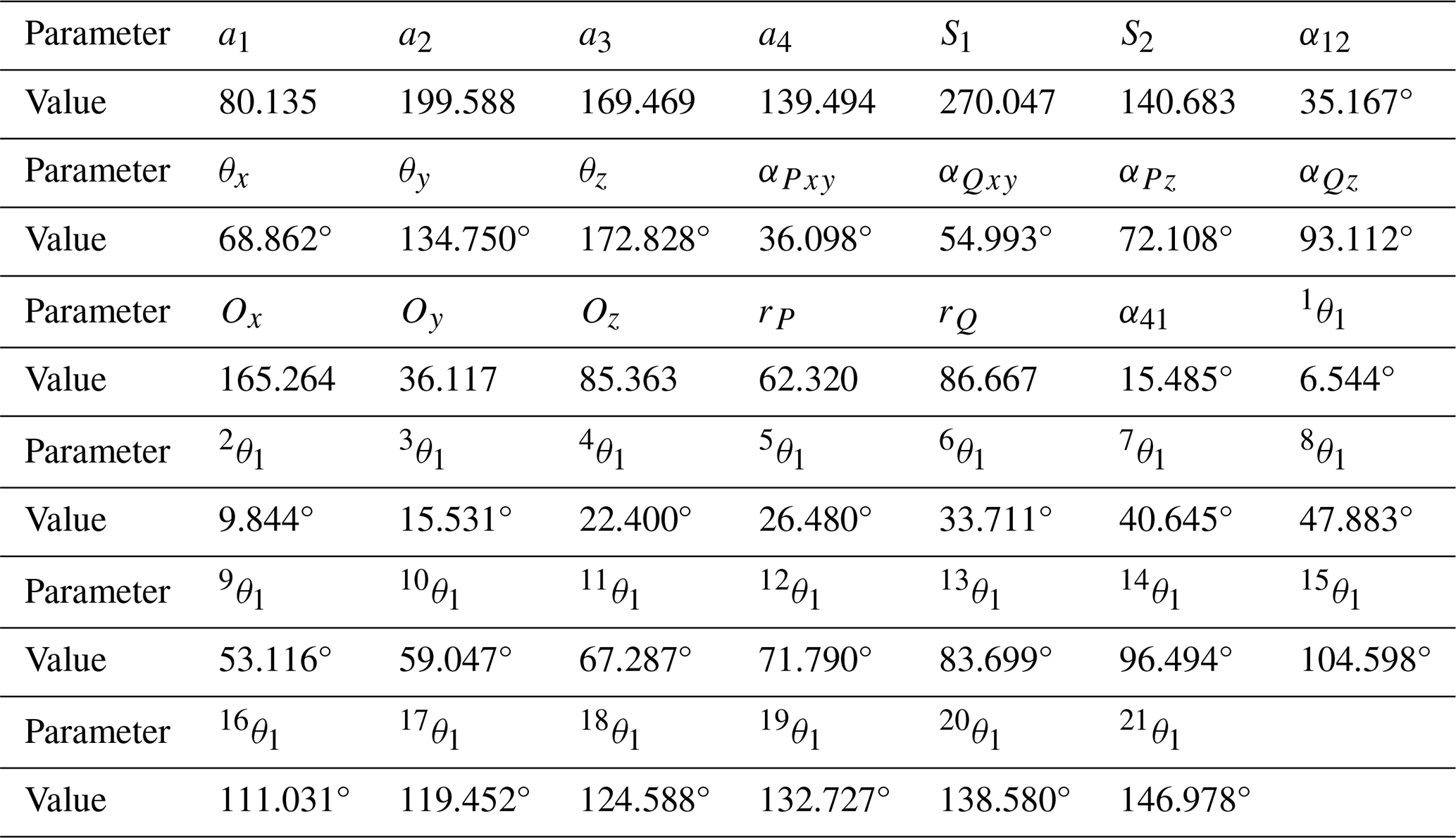
In this section, the proposed spatial RRSC rigid-body guidance mechanism dimensional synthesis method is utilized to solve two cases so as to verify the feasibility and effectiveness of the method. In the first theoretical example, 21 rigid-body guidance lines generated by a spatial RRSC rigid-body guidance mechanism are used as the design requirements for the mechanism so as to validate the correctness of the proposed methodology, as well as the derived computational formulas. In the second example, the rigid-body guidance lines are given in the form of parametric equations.

Table 5 Parameters of the rigid-body guidance lines in Example 1.

5.1 Example 1

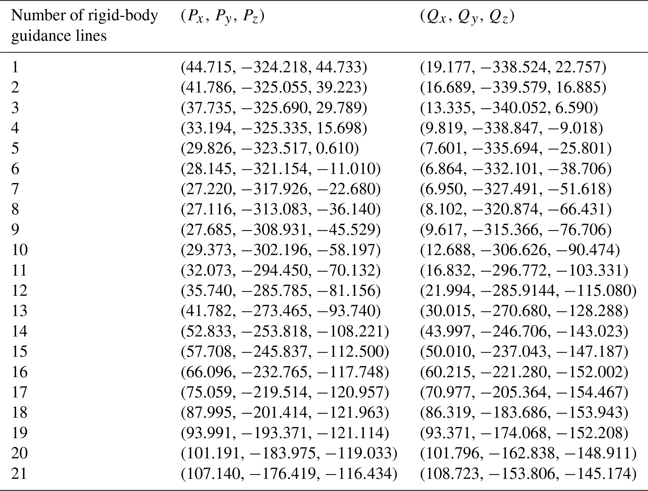
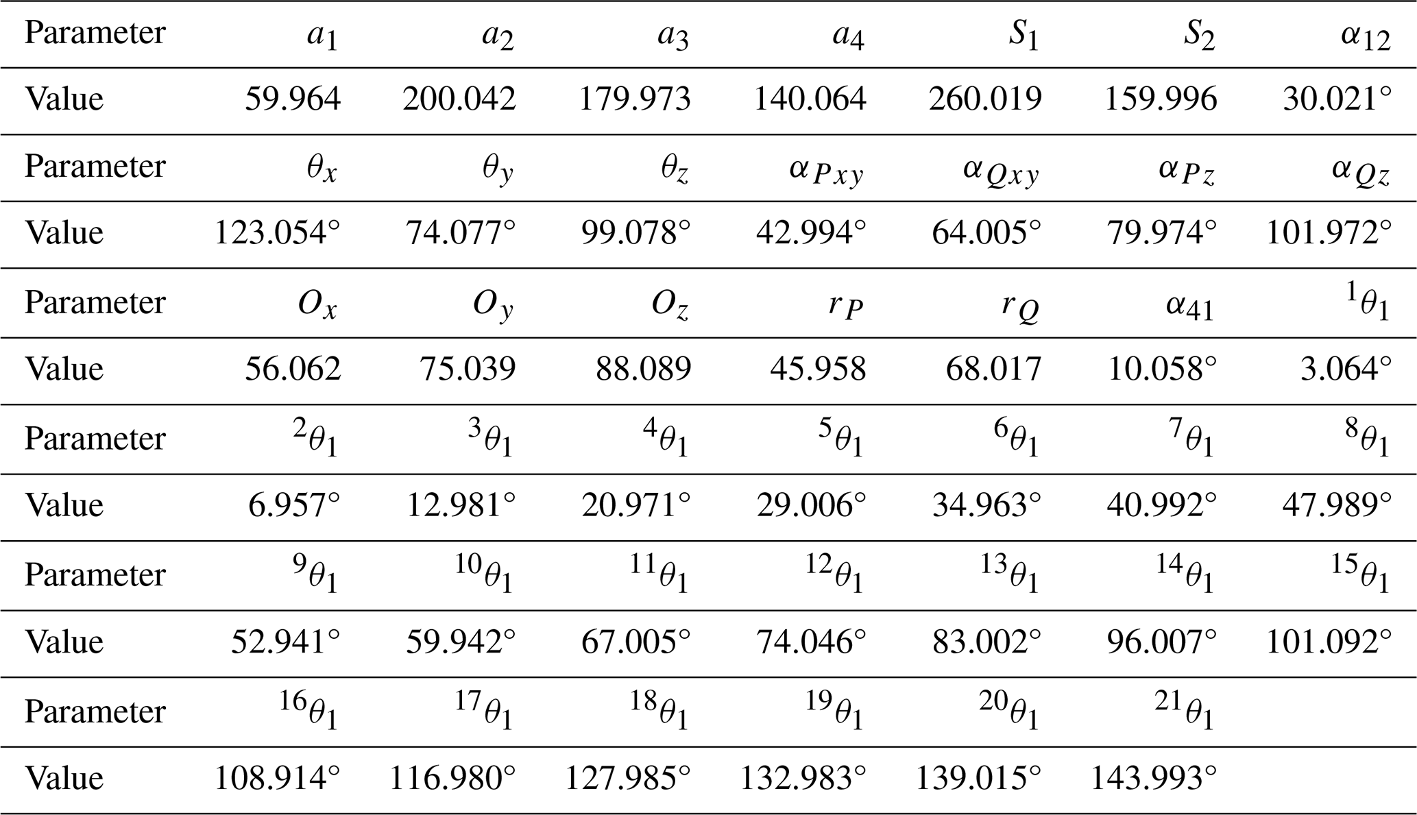
The dimensional parameters of the spatial RRSC rigid-body guidance mechanism are given as follows: a₁=60, a₂=200, a₃=180, a₄=140, S₁=260, S₂=160, α₁₂=30°, and α₄₁=10°. The input angles (θ₁) of the mechanism corresponding to the prescribed rigid-body guidance lines are 3, 7, 13, 21, 29, 35, 41, 48, 53, 60, 67, 74, 83, 96, 101, 109, 117, 128, 133, 139, and 144°, respectively. The position parameters of the coupler points on the rigid-body guidance lines are r_P=46, α_Pxy=43°, α_Pz=80°, r_Q=68, α_Qxy=64°, and α_Qz=102°. The parameters for the installation angle of the mechanism are θ_x=123°, θ_y=74°, and θ_z=99°, and the parameters for the installation position of the mechanism are O_x=56, O_y=75, and O_z=88. According to Eqs. (56) to (61), the coordinates of the coupler points on the rigid-body guidance line can be obtained, and these are listed in Table 5.

To clearly illustrate the calculation process, we take the first input angle θ₁=3° as an example. The coordinates of coupler point P are calculated as follows:

1. With the given geometric parameters a₁=60, a₂=200, a₃=180, a₄=140, S₁=260, S₂=160, α₁₂=30°, and α₄₁=10°, we first calculate the coupler angle θ₂ using Eq. (17). Substituting the values, we get ${}^{\mathrm{1}}{\mathit{\theta }}_{\mathrm{2}}=-\mathrm{21.8079}\mathit{°}$.

2. Subsequently, based on geometric parameters and r_P=46, α_Pxy=43°, α_Pz=80°, r_Q=68, α_Qxy=64°, and α_Qz=102°, the coordinates of point P in the local coordinate system (O_d−x_dy_dz_d), which is a coordinate system attached to the frame, are determined using Eqs. (1) and (2).

   $$\left[\begin{array}{c}{x}_P{(}^{\mathrm{1}}{\mathit{\theta }}_{\mathrm{1}})\\ y_P{(}^{\mathrm{1}}{\mathit{\theta }}_{\mathrm{1}})\\ z_P{(}^{\mathrm{1}}{\mathit{\theta }}_{\mathrm{1}})\end{array}\right]=\left[\begin{array}{c}\mathrm{73.3382}\\ \mathrm{115.5030}\\ \mathrm{148.8498}\end{array}\right]\text{and}\left[\begin{array}{c}{x}_Q{(}^{\mathrm{1}}{\mathit{\theta }}_{\mathrm{1}})\\ y_Q{(}^{\mathrm{1}}{\mathit{\theta }}_{\mathrm{1}})\\ z_Q{(}^{\mathrm{1}}{\mathit{\theta }}_{\mathrm{1}})\end{array}\right]=\left[\begin{array}{c}\mathrm{57.2099}\\ \mathrm{147.7143}\\ \mathrm{142.3601}\end{array}\right]$$

3. The local coordinates are then transformed into the global coordinate system (O_g−x_gy_gz_g) using the installation parameters θ_x=123°, θ_y=74°, θ_z=99°, O_x=56, O_y=75, and O_z=88. The transformation is performed using the rotation matrix

   $$\begin{array}{rl}R& =\left[\begin{array}{ccc}\cos {\mathit{\theta }}_z& -sin{\mathit{\theta }}_z& \mathrm{0}\\ \sin {\mathit{\theta }}_z& \cos {\mathit{\theta }}_z& \mathrm{0}\\ \mathrm{0}& \mathrm{0}& \mathrm{1}\end{array}\right]\left[\begin{array}{ccc}\cos {\mathit{\theta }}_y& \mathrm{0}& \sin {\mathit{\theta }}_y\\ \mathrm{0}& \mathrm{1}& \mathrm{0}\\ -sin{\mathit{\theta }}_y& \mathrm{0}& \cos {\mathit{\theta }}_y\end{array}\right]\\ & \left[\begin{array}{ccc}\mathrm{1}& \mathrm{0}& \mathrm{0}\\ \mathrm{0}& \cos {\mathit{\theta }}_x& -sin{\mathit{\theta }}_x\\ \mathrm{0}& \sin {\mathit{\theta }}_x& \cos {\mathit{\theta }}_x\end{array}\right]\end{array}$$

   and the translation vector

   $$T=\left[\begin{array}{c}{O}_x\\ O_y\\ O_z\end{array}\right].$$

   The local coordinates can be calculated as

   $$\begin{array}{rl}& \left[\begin{array}{c}{x}_{Pg}{(}^{\mathrm{1}}{\mathit{\theta }}_{\mathrm{1}})\\ y_{Pg}{(}^{\mathrm{1}}{\mathit{\theta }}_{\mathrm{1}})\\ z_{Pg}{(}^{\mathrm{1}}{\mathit{\theta }}_{\mathrm{1}})\end{array}\right]=R\left(\left[\begin{array}{c}{x}_P{(}^{\mathrm{1}}{\mathit{\theta }}_{\mathrm{1}})\\ y_P{(}^{\mathrm{1}}{\mathit{\theta }}_{\mathrm{1}})\\ z_P{(}^{\mathrm{1}}{\mathit{\theta }}_{\mathrm{1}})\end{array}\right]+T\right)\\ & =\left[\begin{array}{c}\mathrm{44.7152}\\ \mathrm{324.2177}\\ \mathrm{44.7329}\end{array}\right]\text{and}\left[\begin{array}{c}{x}_{Qg}{(}^{\mathrm{1}}{\mathit{\theta }}_{\mathrm{1}})\\ y_{Qg}{(}^{\mathrm{1}}{\mathit{\theta }}_{\mathrm{1}})\\ z_{Qg}{(}^{\mathrm{1}}{\mathit{\theta }}_{\mathrm{1}})\end{array}\right]\\ & =\text{Rot}\left(\left[\begin{array}{c}{x}_P{(}^{\mathrm{1}}{\mathit{\theta }}_{\mathrm{1}})\\ y_P{(}^{\mathrm{1}}{\mathit{\theta }}_{\mathrm{1}})\\ z_P{(}^{\mathrm{1}}{\mathit{\theta }}_{\mathrm{1}})\end{array}\right]+\text{Trans}\right)=\left[\begin{array}{c}\mathrm{19.1767}\\ \mathrm{338.5237}\\ \mathrm{22.7574}\end{array}\right].\end{array}$$

   The calculated result matches the first row of data in Table 6.

Table 6 Design results of Example 1.

Table 7 Design results for calculation Example 2.

This step-by-step computation verifies the validity of the transformation equations. The coordinates of the coupler points for all other rigid-body guidance lines listed in Table 6 are obtained following the same procedure.

Figure 8 Design results for Example 2.

Figure 9 Error of Example 2.

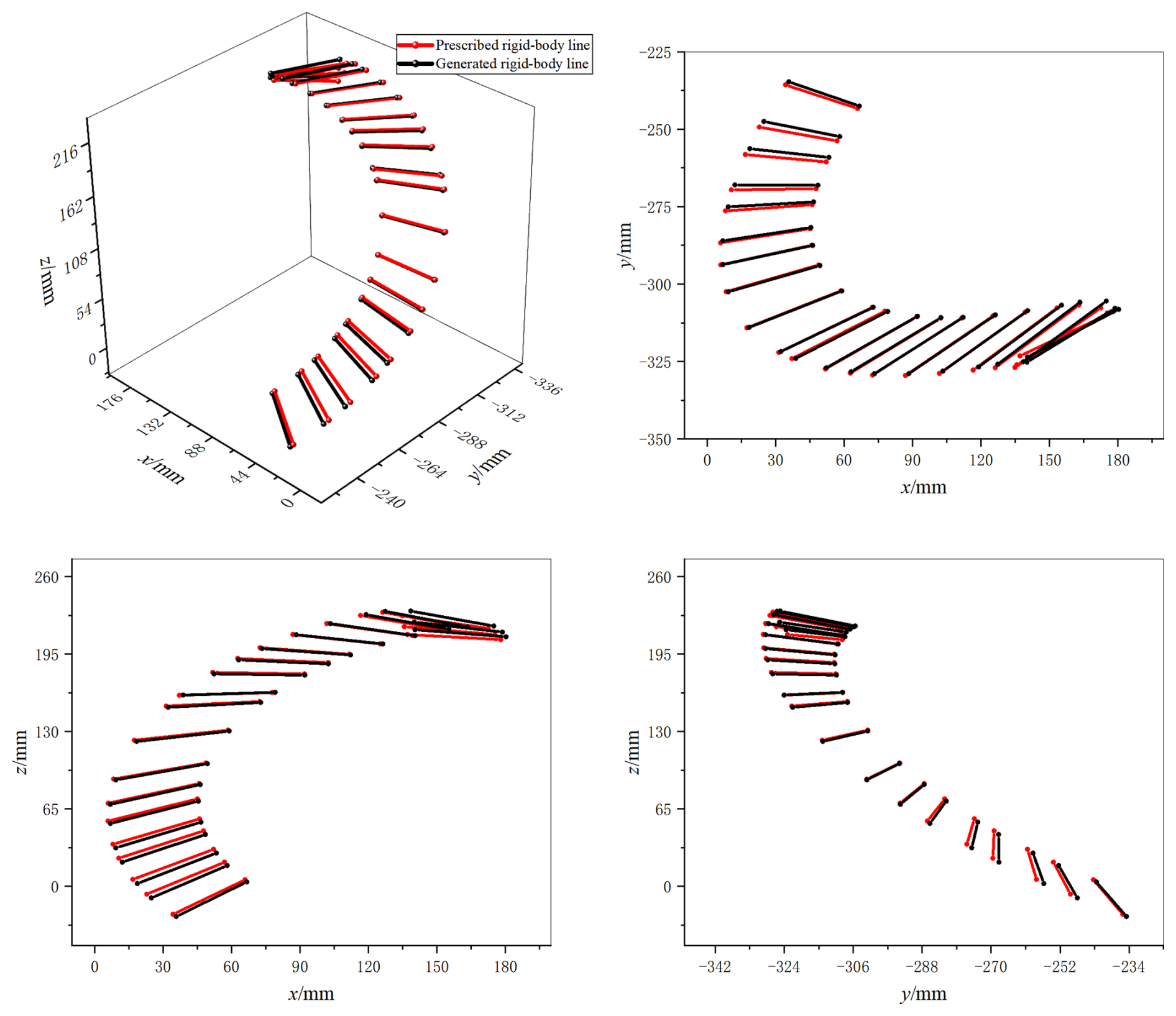
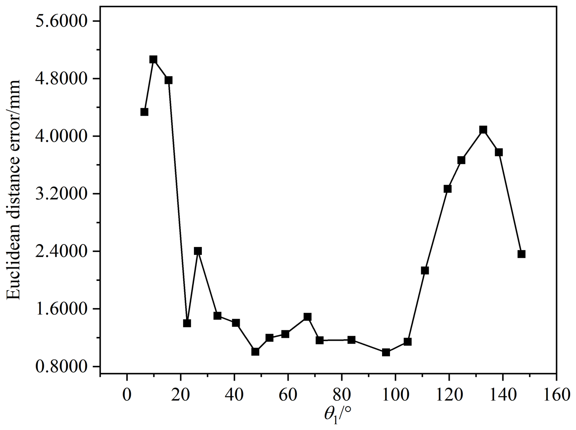
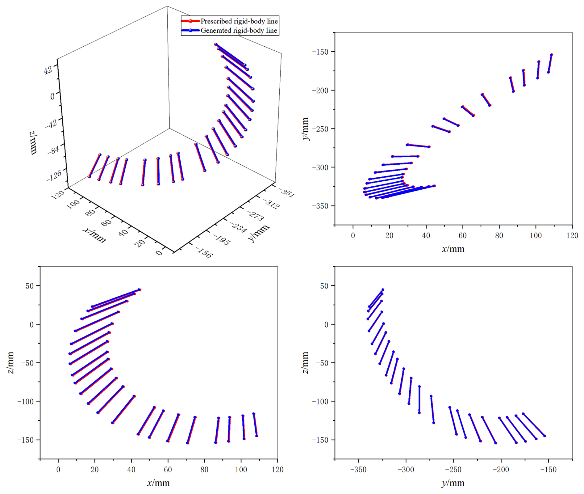
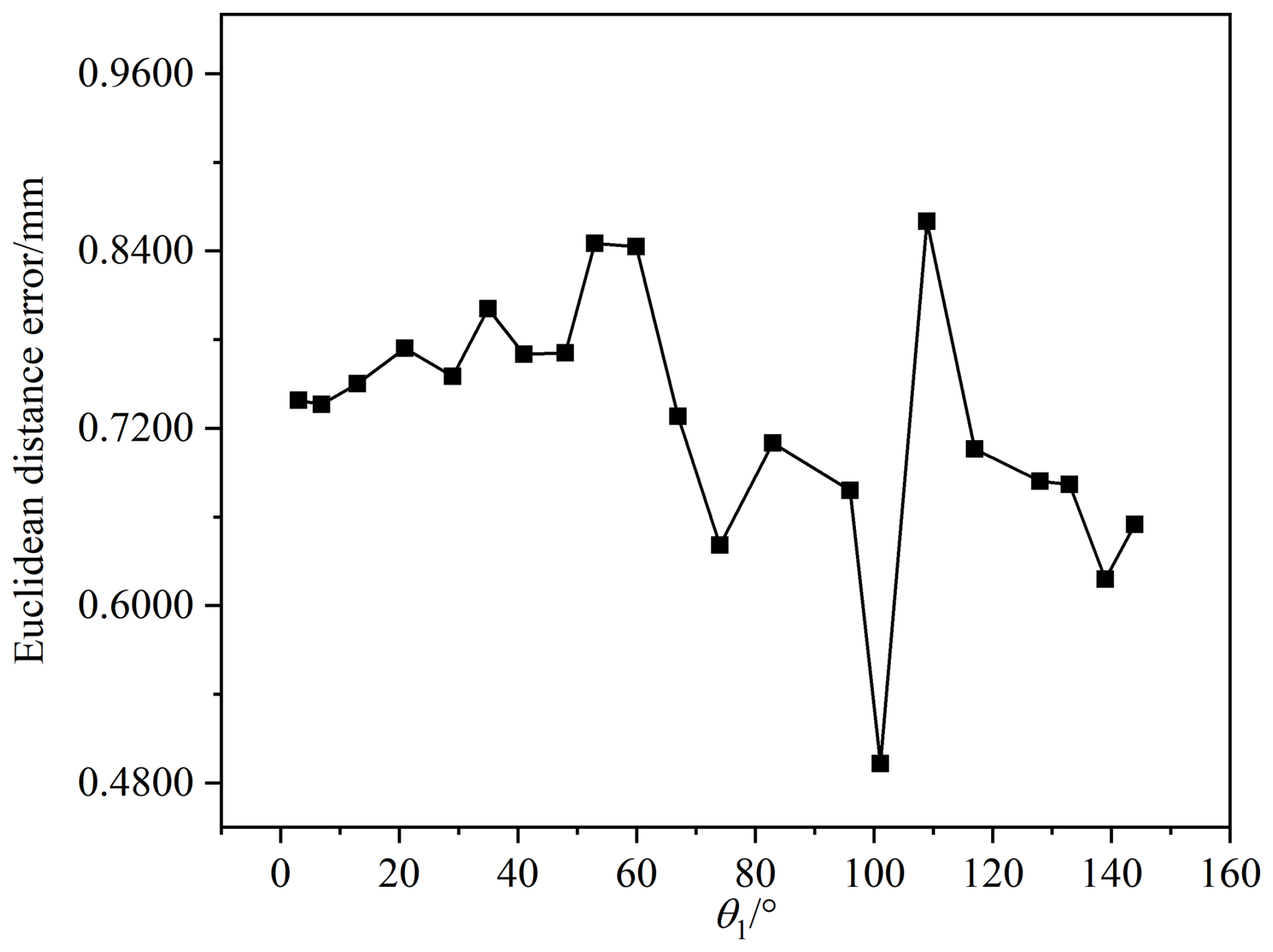
According to the proposed method, two databases are established to match and identify the parameters. First, using the installation angle parameter database, the installation angles (θ_x, θ_y, and θ_z), initial input angle (¹θ₁), and α₁₂ are obtained, and the running time of the process is 412.28 s. Second, the basic dimensional types of the desired mechanism are matched using the basic dimensional type database, and the running time of the process is 386.42 s. Third, the installation parameters and dimensional parameters of the RRSC rigid-body guidance mechanism were obtained based on the theoretical formulas derived for the actual dimensions of the mechanism, and the running time is 0.74 s. Finally, the obtained mechanism parameters are used as initial values to optimize the mechanism geometric parameters using the genetic algorithm, and the running time of optimization process is 1.04 s. The design results and the projections of the rigid-body guidance lines of the target mechanism on the x_gO_gy_g, x_gO_gz_g, and y_gO_gz_g planes are shown in Fig. 6. The error conditions are shown in Fig. 7. All dimensional parameters are shown in Table 6. Comparing the dimensional parameters of the prescribed mechanism and the mechanism generated by the design results, it is obvious that they are basically the same. This demonstrates the feasibility and effectiveness of the method we propose.

5.2 Example 2

In this section, the target rigid-body guidance lines are generated by the following expression:

$$\begin{array}{rl}& x_Q=\mathrm{1185}\sin \left(\mathrm{0.7763}\mathit{\theta }-\mathrm{0.4836}\right)+\mathrm{1178}\sin (\mathrm{0.8234}\mathit{\theta }+\mathrm{2.52}),\\ & y_Q=\mathrm{5386}\sin \left(\mathrm{0.3619}\mathit{\theta }-\mathrm{4.545}\right)+\mathrm{5060}\sin (\mathrm{0.366}\mathit{\theta }+\mathrm{1.411}),\\ & z_Q=\mathrm{211.3}\sin \left(\mathrm{0.4157}\mathit{\theta }-\mathrm{1.587}\right)+\mathrm{32.91}\sin (\mathrm{1.501}\mathit{\theta }+\mathrm{0.1883}),\\ & \mathit{\psi }=\mathrm{2.756}\sin \left(\mathrm{0.6278}\mathit{\theta }-\mathrm{0.2119}\right)+\mathrm{1.442}\sin (\mathrm{0.9051}\mathit{\theta }+\mathrm{2.398}),\\ & \mathit{\eta }=\mathrm{0.9447}\sin \left(\mathrm{1.125}\mathit{\theta }-\mathrm{0.1163}\right)+\mathrm{0.5198}\sin (\mathrm{1.415}\mathit{\theta }+\mathrm{2.353}),\end{array}$$

where θ is a variable (in this algorithm, θ is taken from 10 to 210° with a step size of 10); x_Q, y_Q, and z_Q are the coordinates of the sampling point Q on the prescribed rigid-body guidance line; ψ is the angle between the rigid-body guidance line PQ and the z axis on the global coordinate system; and η is the angle between the projection of the rigid-body guidance line PQ on the xOy plane and the x axis on the global coordinate system. Using the method proposed in this paper, the dimensional synthesis of spatial RRSC rigid-body guidance mechanisms is realized. The design results are presented in Table 7. Figure 8 shows the mechanism generated by the design results and the projections of the rigid-body guidance lines of the target mechanism on the x_gO_gy_g, x_gO_gz_g, and y_gO_gz_g planes, and the error is shown in Fig. 9. The running time of the synthesis process is 788.32 s. The time consumption for each specific step is as follows: step 1, which involves matching the installation angle parameters, took 426.15 s; step 2, which involves matching basic dimensional types, took 360.11 s; step 3, which involves calculating other mechanism parameters, took 0.85 s; and step 4, which involves optimizing all parameters, took 1.21 s.

For comparison, we conduct a full-parameter optimization for the desired mechanism using a pure optimization method. The optimization involved 41 dimensions (21 mechanism parameters, namely a₁, a₂, a₃, a₄, S₁, S₂, α₁₂, θ_x, θ_y, θ_z, α_Pxy, α_Qxy, α_Pz, α_Qz, O_x, O_y, O_z, r_P, r_Q, α₄₁, and ¹θ₁, and 20 input angles, namely ²θ₁, ³θ₁, …, ²⁰θ₁, and ²¹θ₁). To ensure a fair comparison with the method proposed in this paper, we used the same genetic algorithm parameters and executed 100 optimization runs. The best result achieved a mean Euclidean distance error exceeding 50 mm, which is more than 15 times larger than the error obtained by our proposed method. Furthermore, we increased the population size to 50 000 and the number of generations to 500. Due to the significantly increased computational burden, we performed only 10 runs under this configuration. Even with these expanded resources, the best result still exhibited a mean Euclidean distance error of over 30 mm, which is more than 10 times greater than the error achieved by our method.

6 Conclusions

In this paper, the dimensional synthesis of spatial RRSC rigid-body guidance mechanisms for multi-position unprescribed-timing design requirements is investigated. First, based on the relationship among spatial rigid-body guidance mechanisms in standard, deflected, and general installation positions, the timing supplementation method developed for mechanisms in a standard installation position is extended to those in general installation positions. Second, by analysing the structural parameter characteristics of the feature coupler circle, a method for extracting the relative coupler angle of the desired mechanism is presented. Based on the basic idea of the numerical atlas method, a six-dimensional database of basic dimensional mechanism types is established, and the geometric parameters of the target mechanism are determined through matching and identification. Theoretical formulas for calculating the actual dimensions of the mechanism are then derived.

The proposed method fills a gap in existing numerical atlas methods, which have not previously addressed dimensional synthesis for unprescribed-timing constraints. Moreover, our approach solves the 21-D motion generation problem for spatial RRSC mechanisms in several steps. Therefore, it offers unique advantages: it does not require a large pre-established numerical atlas database, enables fast matching and recognition, and achieves high accuracy in design results. It also addresses the shortcomings of approximate synthesis methods – such as unstable accuracy and difficulty in guaranteeing convergence of the optimization algorithm.

Although the step-by-step process significantly reduces computational complexity by decomposing the 21-parameter problem into smaller subproblems, this sequential approach increases the risk of converging to a local rather than the global optimum. Regarding this issue, an optimization method is applied to refine the dimensional parameters of the mechanism, thereby achieving dimensional synthesis of the spatial RRSC rigid-body guidance mechanism under multi-position unprescribed-timing design requirements. However, even with this refinement, the solution may not represent the global optimum; moreover, it reduces efficiency.

Due to the high dimensionality and inherent randomness in the optimization of spatial mechanisms, further improving solution precision and developing global optimization algorithms that are computationally feasible remain important directions for future research.

Appendix A: Nomenclature

Og−xgygzg	The global coordinate system
Od−xdydzd	The coordinate system attached to the frame
O′-$x^{\prime }{y}^{\prime }{z}^{\prime }$	The coordinate system attached to the input link
O′′-x′′y′′z′′	The coordinate system attached to the coupler link
a1, a2, a3, a4, S1, S2 and S3	The lengths of links AB, CD, DE, FG, GA, BC,
	and EF
LDF	The distance from point D to point F
α12	The angle between the rotation axis of the input link
	and the rotation axis of the coupler link
α41	The angle between the rotation axis of the driven link
	and the rotation axis of the input link
θ1 and θ2	The input angle and coupler angle
rP and rQ	The lengths of links CP and CQ
αPxy	The angle between the x′ axis and the projection
	of CP on the $x^{\prime }{O}^{\prime }{y}^{\prime }$ plane
αQxy	The angle between the x′ axis and the projection
	of CQ on the $x^{\prime }{O}^{\prime }{y}^{\prime }$ plane
αPz	The angle between CP and the z′ axis
αQz	The angle between CQ and the z′ axis
Ox,Oy, and Oz	The installation position parameters
θx, θy, and θz	The installation angle parameters
P and Q	The coupler points
P′and Q′	The points obtained by rotating the coupler points
	P and Q clockwise around the zd axis by the
	input angle
P′′ and Q′′	The points obtained by rotating the points P′
	and Q′ clockwise around the xd axis by α12
⊙P and ⊙Q	The feature coupler circles
RP and RQ	The radii of ⊙P and ⊙Q
$O_{P^{\prime \prime }}$ and $O_{Q^{\prime \prime }}$	The origin coordinates of ⊙P and ⊙Q
xP, yP, and zP	The coordinates of point P
xQ, yQ, and zQ	The coordinates of point Q
xD, yD, and zD	The coordinates of point D
xF, yF, and zF	The coordinates of point F
xP′, yP′, and zP′	The coordinates of point P′
xQ′, yQ′, and zQ′	The coordinates of point Q′
xP′′, yP′′, and zP′′	The coordinates of point P′′
xQ′′, yQ′′, and zQ′′	The coordinates of point Q
xPg, yPg, and zPg	The coordinates of point P in a general installation
	position on a spatial RRSC rigid-body guidance
	mechanism, defined within the global coordinate
	system Og−xgygzg
xQg, yQg, and zQg	The coordinates of point Q in a general installation
	position on a spatial RRSC rigid-body guidance
	mechanism, defined within the global coordinate
	system Og−xgygzg
xPc, yPc, and zPc	The coordinates of the closest feature coupler
	point P′′ on the feature coupler
	circles ⊙P
xQc , yQc, and zQc	The coordinates of the closest feature coupler point
	Q′′ on the feature coupler circles ⊙Q
θFCCP and θFCCQ	The feature central angles
w1, w2, w3, w4,	The intermediate variables
w5, w6, v1, v2, v3,
Δ, Δ1, Δ2, a,b,
c,d,e,f, b2,b3,
b4, c2,c3, c4,b5,
b6, b7, k, τ, d1,
d2, e1, e2, f1, g,
h, i, p, q,r, s, w, and u
δ and δ2	The error functions
FCC	The abbreviation for feature coupler circle