Design, modeling and manufacture error identification of a new 6-degree-of-freedom (6-DOF) compliant parallel manipulator

This paper introduces a new 6-degree-of-freedom (6-DOF) compliant parallel manipulator featuring a 6-prismatic, spherical, spherical (6-PSS) configuration, leaf spring compliant joints and manufacture error identification techniques, which collectively enhance motion accuracy, motion range and dynamic performance. The 6-PSS configuration allows actuators to be mounted on the base frame rather than on the moving parts of the manipulator, thereby improving their dynamic performance. The use of leaf spring compliant joints offers superior accuracy over traditional rigid joints due to the absence of backlash and provides a relatively large motion range compared to typical compliant joints with lumped compliance. The kinetostatic models of these compliant joints have been derived and closely align with the finite-element model, exhibiting an average difference of approximately 5.5 %. Additionally, a kinematic model of the whole manipulator has been formulated and, based on it, a manufacture error identification model has been established to identify the manufacture errors, which is crucial for improving the motion accuracy. The Levenberg–Marquardt optimization algorithm is utilized to solve the identification model, with the results verified through finite-element analysis. The proposed 6-DOF compliant parallel manipulator shows great promise for applications in precision engineering, such as optical guidance and chip packaging.

1 Introduction

Six-degree-of-freedom (6-DOF) manipulators play an important role in various engineering fields owing to their dexterous motion capabilities. They are utilized in diverse applications, encompassing the assembly of engines, wings and satellites (Gonzalez and Asada, 2017), precise positioning and packaging of chips (Jeong et al., 2007) and high-precision operations for minimally invasive surgery (Ma et al., 2019). As the relevant application sectors evolve, the demand for 6-DOF manipulators in terms of accuracy, motion range, dynamic performance and lightweight design will continue to grow (Wu and Niu, 2024; Fang et al., 2023). Typically, 6-DOF manipulators employ either serial or parallel configurations (Campos et al., 2008; Alizade et al., 2007). The serial configuration features motion chains connected in sequence to form an open chain and offers a wide working range and high dexterity in handling complex tasks (He et al., 2010). However, this configuration suffers from lower dynamic performance and load capacity, with a consequent reduction in motion accuracy due to the accumulation of errors. In contrast, the parallel configuration, with motion chains arranged in parallel between the base and the moving platform, possesses a relatively high load capacity, dynamic performance and motion accuracy (Hou et al., 2019; Jin et al., 2015; Tsai, 1999). In conclusion, 6-DOF manipulators with parallel configurations outperform their serial counterparts in both motion accuracy and dynamic performance. Hence, this paper focuses on the design of a 6-DOF manipulator utilizing a parallel configuration, here referred to as a 6-DOF parallel manipulator.

Traditional 6-DOF parallel manipulators with rigid joints often face challenges in preserving accuracy due to factors like friction, wear and backlash of joints. In contrast, 6-DOF compliant parallel manipulators utilize elastic deformation of materials to transfer force and displacement. These manipulators require no lubrication, suffer less friction, and exhibit no backlash, thus achieving higher motion resolution and accuracy. Consequently, they are widely used in precision engineering fields (Howell, 2013). For instance, Du et al. (2014) applied a three-axis compliant circular notch joint to a high-precision 6-DOF manipulator for inter-satellite optical communication, achieving sub-micrometer resolution and a sub-millimeter pointing range with micro-radian repeatability. Xu et al. (2021) employed slender beam compliant joints in a 6-DOF manipulator designed for the optical alignment of optoelectronic devices. Similarly, Dan and Rui (2016) used slender beam compliant joints to design a 6-DOF compliant parallel manipulator for micro-positioning applications, where its working precision could be further improved by reducing the workspace. For ultra-high-precision engineering applications, Qi et al. (2023) designed a 6-DOF compliant parallel manipulator and introduced a novel modeling method aimed at addressing the challenges of establishing the relationship between the input voltage and output position. Yang et al. (2019) utilized a 6-DOF compliant manipulator for high-precision spatial system isolation, demonstrating its excellent accuracy and vibration isolation performance through simulation and experimentation. Therefore, while 6-DOF compliant parallel manipulators demonstrate significant promise in precision engineering, ongoing improvements in their accuracy, motion range and dynamic performance are crucial for advancing precision engineering technologies. Building on the above statements, it is advantageous to design a 6-DOF parallel manipulator with compliant joints, referred to as a 6-DOF compliant parallel manipulator, to further the enhance accuracy, expand the motion range, and improve the dynamic performance.

During the manufacturing process of 6-DOF compliant parallel manipulators, the existence of fabrication and assembly errors causes slight deviations between theoretical and actual geometric parameters. These deviations propagate along each chain to the moving platform, leading to deviations in its actual motion trajectory from the ideal one and reducing the motion accuracy. Kinematic calibration can resolve this issue by incorporating manufacture error identification modeling and dimension measurement, solving the manufacture error identification model and compensating for manufacture errors. Numerous scholars have researched manufacture error identification modeling. For example, Denavit and Hartenberg (1955) proposed the classical D–H differential matrix method, establishing a kinematic relationship between the moving platform and base through coordinate transformations among the joints. Nahvi et al. (1994) adopted the closed-loop vector method to establish the manufacture error identification model for a parallel mechanism, which is widely applied in error identification modeling for such parallel mechanisms due to its clear and concise expression. In contrast to these linear modeling methods, nonlinear optimization algorithms can directly identify geometric parameter errors. Alıcıet al. (2006) employed a particle swarm optimization algorithm, inputting dimension measurement data into a manufacture error estimation function to accurately identify manufacture errors in geometric dimensions. In this paper, selecting an appropriate manufacture error identification modeling method is pivotal for accurately identifying manufacture errors, considering that compliant joints are involved.

This paper introduces a new 6-DOF manipulator with a parallel configuration, leaf spring compliant joints and manufacture error identification technologies capable of achieving high precision, a relatively large motion range and high dynamic performance. The main contributions and novelties of this paper include (1) proposing a new 6-DOF compliant parallel manipulator featuring a 6-prismatic, spherical, spherical (6-PSS) configuration and leaf spring compliant joints, which ensures high precision, high load capacity, large motion ranges and superior dynamic performance, and (2) identifying manufacture errors of the proposed 6-DOF compliant parallel manipulator to further improve motion accuracy. In addition to these innovations, this paper also undertakes the following tasks: (1) deriving the forward and inverse kinematic models of the entire manipulator using the closed-loop vector method and Newton iteration method and (2) establishing kinetostatic models of the complex compliant joints using the matrix displacement method.

The remainder of this paper is organized as follows. Section 2 introduces the synthesis of the 6-DOF parallel manipulators with compliant joints. Section 3 establishes the kinematic model of the 6-DOF compliant parallel manipulator. Section 4 constructs and validates the kinetostatic model of the compliant joints. Section 5 identifies the manufacture errors in the geometric parameters. The main conclusions of this paper are drawn in Sect. 6.

2 Mechanism synthesis

In this section, the configuration of the 6-DOF compliant parallel robot is synthesized. The advantages and disadvantages of common 6-DOF parallel configurations and compliant joints are analyzed, selecting the optimal configuration based on the design requirements. A 3D model of the 6-DOF compliant parallel manipulator is established, and a preliminary motion simulation using the finite-element method (FEM) is conducted to validate the rationality of the design.

2.1 Configuration selection

The main configurations employed in parallel mechanisms are illustrated in Fig. 1. In the 6-revolute, universal, spherical (6-RUS) configuration as shown in Fig. 1a, the revolute pairs are directly actuated by rotary actuators that are mounted on the base frame, enhancing the dynamic performance. However, its large size is a disadvantage for miniaturization and is lightweight. In a typical configuration, such as the 6-spherical, prismatic, spherical (6-SPS) depicted in Fig. 1b, actuators are positioned on the legs, which increases the mass of the moving parts and decreases the response speed. To address these issues, actuators can be fixed to the base in a 6-PSS configuration. This configuration encompasses three main types: orthogonal drives, circumferential lateral drives and circumferential vertical drives. The orthogonal configuration, depicted in Fig. 1c, forms a cubic shape, dividing the six legs into three groups, with each group's translational joints mounted vertically on the base. This design streamlines assembly and demonstrates isotropic characteristics of motion and force transmission. It also allows decoupling of deformations under actuation forces, making it suitable for multi-axis force sensor structures. However, the circumferential lateral drive type illustrated in Fig. 1d possesses a large base area, resulting in a less compact structure. In contrast, the vertical drive type, as shown in Fig. 1e, reduces the overall size, decreases the mass of the moving parts, and mitigates additional load on the mechanism, thereby enhancing its response speed. Therefore, this paper adopts 6-PSS parallel configurations based on circular vertical drives for innovative design.

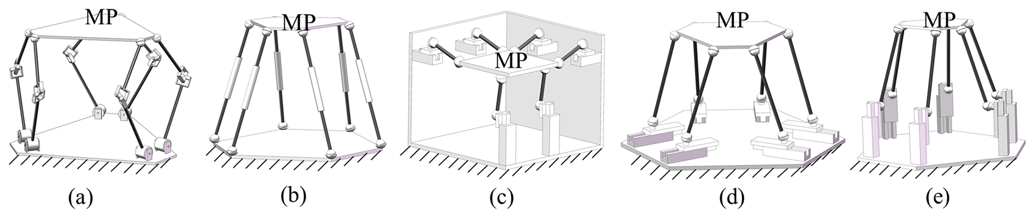
Figure 1 Schematic overview of the five configurations of 6-DOF parallel manipulators, with MP as the moving platform: (a) 6-RUS configuration, (b) 6-SPS configuration, (c) 6-PSS configuration (orthogonal), (d) 6-PSS configuration (lateral drive), and (e) 6-PSS configuration (vertical drive).

A schematic diagram of the mechanism based on the circular vertical-drive 6-PSS parallel configuration is shown in Fig. 2a, primarily comprising a base, a moving platform, translational joints, spherical joints, and six legs, with the base rigidly connected to the ground. Each leg, denoted as A_iB_i, connects the upper and lower spherical joints. The upper spherical joint centers A_i are arranged along a circle termed the upper joint circle, while the lower spherical joints connect to the translational joints fixed on the base, forming a circle at their centers B_i that is referred to as the lower joint circle. As shown in Fig. 2b, the six upper joint points A_i form a symmetrical hexagon with equal long and short sides divided into three groups spaced 120° apart. The distribution of the lower joint points mirrors that of the upper ones. The lines connecting the upper and lower joint points form two symmetrical hexagons spaced 180° apart. In addition, it can be seen from Fig. 2c that the lines connecting the origin of the base O_B, the origin of the moving platform O_A and the spherical joint A_i and B_i form a closed-loop vector. The configuration parameters of the parallel manipulator include the distribution radius of the moving platform's joint points r_A (i.e., the radius of the upper joint circle), the distribution radius of the base joint points r_B (i.e., the radius of the lower joint circle), the central angles of the upper and lower joint point distributions θ_A and θ_B, the leg length L and the overall height of the mechanism H.

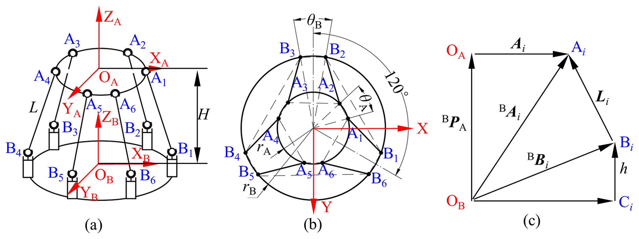
Figure 2 Schematic diagram of the 6-PSS configuration: (a) schematic diagram of the configuration, (b) top view of the joint distribution and (c) vector diagram of the chain.

2.2 Compliant joint synthesis

Compliant spherical joints can be classified into two main types: lumped compliance and distributed compliance. Compared to lumped-compliance compliant spherical joints, those with distributed compliance offer a larger range of motion, less stress concentration and a lower risk of fatigue damage. Figure 3 displays five design schemes for distributed-compliance compliant spherical joints. In Fig. 3a (Hao et al., 2024), the compliant spherical joint comprises three I-shaped leaf springs evenly spaced around a circle, which, due to rotational symmetry, minimizes parasitic and coupling movements associated with the three principal rotations. However, this design suffers from limited supporting stiffness. Figure 3b (Rommers et al., 2021) shows a compliant spherical joint formed by three nested tetrahedral elements, each differing in size and shape to ensure the coincidence of the rotation center. The design in Fig. 3c (Rommers et al., 2021) includes tetrahedral elements configured as two arms set at a specific angle, with each arm made up of four tetrahedral elements in series, thereby extending the motion range and preventing collisions. The extended lines of all the tetrahedral element edges intersect at a distant rotation center. Both compliant joints can be manufactured through 3D printing, which simplifies the manufacturing but constrains the motion range. The compliant spherical joint in Fig. 3d (Parvari et al., 2018) consists of two identical open chains connected in parallel, featuring coincident curvature centers and orthogonal minimum rotational stiffness axes. Each open chain comprises three identical circular compliant beams, symmetrically arranged relative to the curvature center of the beam and providing fully isotropic behavior. However, this design has a larger volume and is not compact enough, which is disadvantageous for miniaturization. The compliant spherical joints described above have limitations, e.g., a small motion range, insufficient supporting stiffness and a bulky design. To address these issues, Naves et al. (2019) proposed a large-range compliant spherical joint based on stacked folded leaf springs, as shown in Fig. 3e. This design maintains high support stiffness over a ±30° tip tilt around the x and y axes and a ±10 ° tip tilt around another axis. It mainly consists of a base, folded leaf springs and an intermediate body. As illustrated in Fig. 4, the compliant spherical joint comprises two sets of folded leaf springs stacked in parallel around a circle that are symmetrical about a plane perpendicular to the rotation axis. To prevent collisions between the leaf springs, one set is rotated a certain angle τ around the symmetry axis. This design means that each set of folded leaf springs contributes only half of the motion, reducing the stress level in the bending section and increasing the support stiffness. Each set of three folded leaf springs has a fold line inclined at a certain angle θ, intersecting at one point to ensure the coincidence of the instantaneous rotation center. Each folded leaf spring connects at its ends to the base and the intermediate body, with the overall height of the compliant spherical joint denoted as h₁.

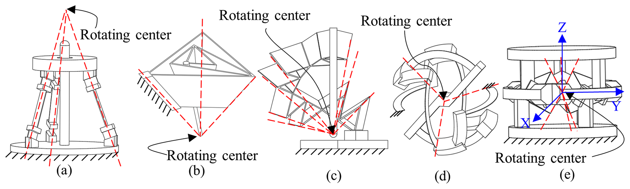
Figure 3 Compliant spherical joints: (a) I-shaped leaf spherical joint, (b) tetrahedral nested spherical joint, (c) tetrahedral series spherical joint, (d) annular leaf spherical joint and (e) folded leaf spring spherical joint.

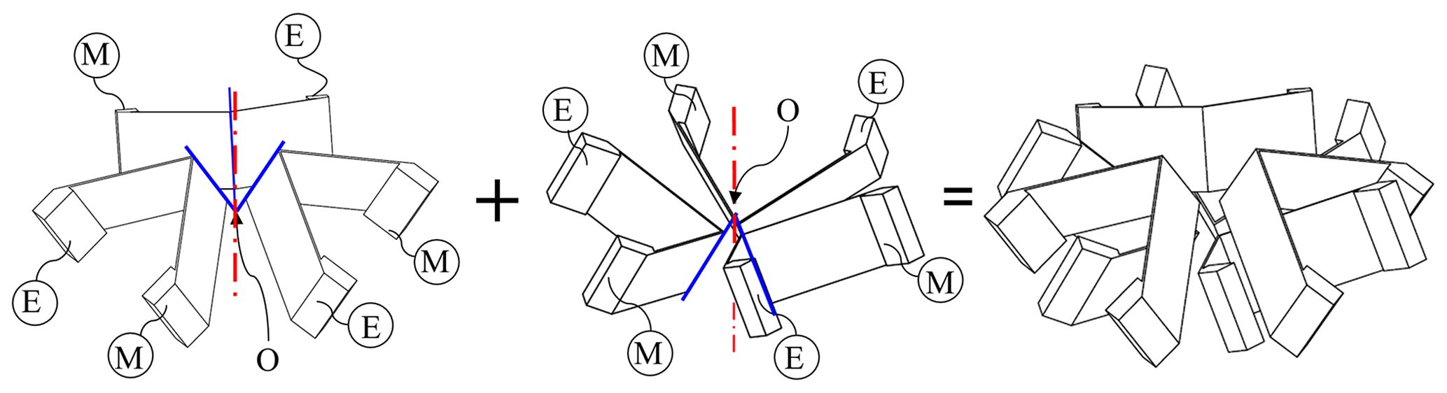
Figure 4 Folded leaf springs in parallel stacking (the M end attached to the intermediate body and the E end to the base).

Figure 5 Common parallelogram compliant translational joints. OT stands for the output stage. (a) Basic parallelogram mechanism (BPM), (b) compound basic parallelogram mechanism (CBPM), (c) double-parallelogram mechanism (DPM) composed of two BPMs in embedded series and (d) compound double-parallelogram mechanism (CDPM) composed of two DPMs in mirror symmetry.

To ensure that the motion direction of the actuator remains consistent and supports the weight of the mechanism, a compliant translational joint is designed to constrain the motion of the actuator. Figure 5 illustrates four common parallelogram compliant translational mechanisms: the basic parallelogram mechanism (BPM), compound basic parallelogram mechanism (CBPM), double-parallelogram mechanism (DPM) and compound double-parallelogram mechanism (CDPM). Compared to the other designs, the BPM is prone to undesired translational parasitic motions. In contrast, the CBPM, formed by mirroring two BPMs, does not produce parasitic motion; however, its main stiffness increases significantly as translational motion progresses due to the load-strengthening effect that restrains the parasitic motion. In addition, the DPM and CDPM offer a large motion range. They introduce an uncontrollable secondary module that reduces off-axis translational stiffness and can lead to dynamic issues. Consequently, the compliant translational joint in this paper is designed based on the CBPM, comprising leaf springs and connecting rigid-body blocks featuring a hexahedral shape and symmetry.

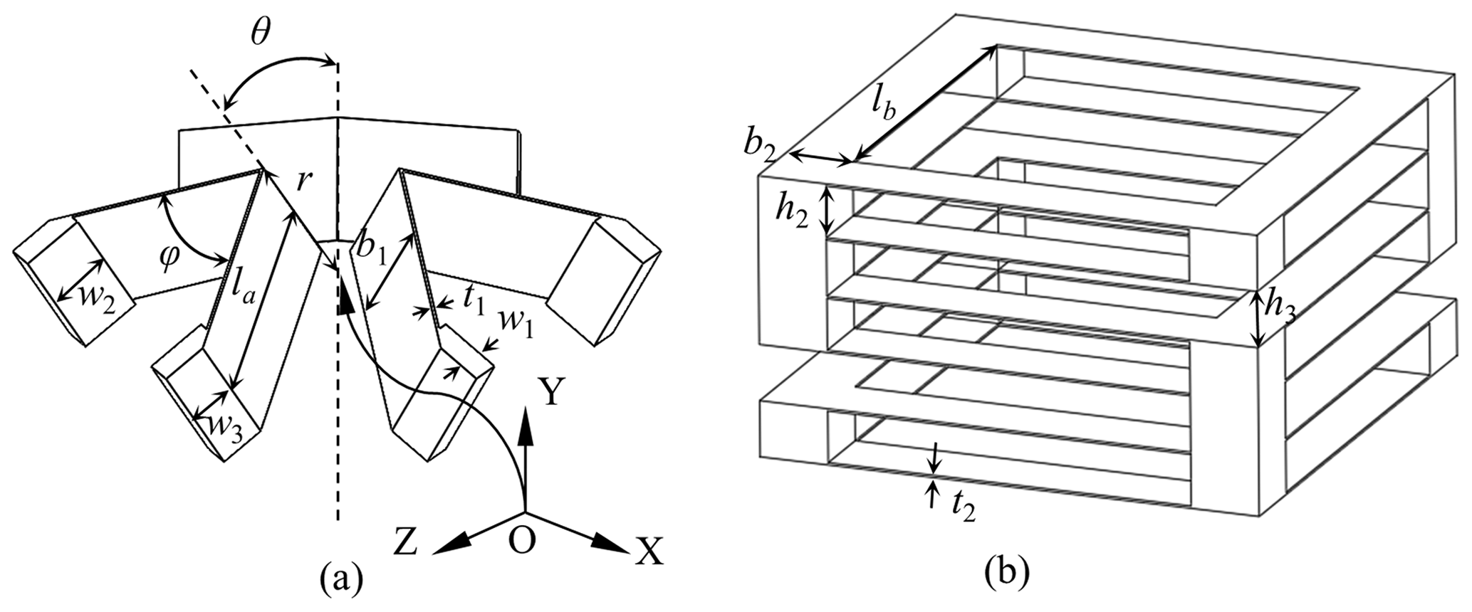
Figure 6 Geometric parameters of the compliant joints: (a) geometric parameters of the compliant spherical joint and (b) geometric parameters of the compliant translational joint.

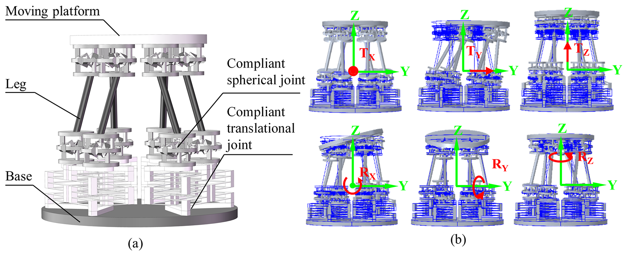
Figure 7 Three-dimensional model of the 6-DOF manipulator and preliminary motion simulation results: (a) 3D model of the 6-DOF compliant parallel manipulator and (b) simulation results of the 6-DOF motion of the 6-DOF compliant parallel manipulator.

The geometric dimensions of the compliant spherical joint and the compliant translational joint used in this paper are shown in Fig. 6. Twenty-four leaf springs are divided into four groups, distributed on four sides of the hexahedron, forming a closed “S” shape with each group of connecting blocks. Following the completion of all the configuration syntheses, the 3D model of the 6-DOF compliant parallel manipulator is obtained, as shown in Fig. 7a. To validate the design rationality of the proposed 6-DOF compliant parallel manipulator, the motion simulation is conducted using the COMSOL5.3 software, with the results presented in Fig. 7b.

3 Kinematic modeling of the 6-DOF manipulator

To analyze the designed 6-DOF compliant parallel manipulator, kinematic modeling is required. In this section, the closed-loop vector method is used for inverse kinematics analysis of the 6-DOF compliant parallel manipulator, while the Newton iteration method is employed to solve the forward kinematics problems. In addition, by establishing the relationship between input displacement and output displacement, a foundation is provided for subsequent manufacture error identification of the manipulator.

3.1 Inverse kinematics

After establishing the configuration of the 6-DOF parallel manipulator and defining the moving coordinate system O_A–X_AY_AZ_A and the fixed coordinate system O_B–X_BY_BZ_B (as shown in Fig. 2), the position, orientation and motion relationship of each component within the fixed coordinate system can be described through the transformation relationship between the moving and fixed coordinate systems.

The position of the moving platform origin O_A in the fixed coordinate system is denoted as ^BP_A= ($x,y,z$), and the orientation of the moving platform relative to the base is denoted as ^B θ_A= (α, β, γ). Here, α represents the rotation angle of the coordinate system {O_A} around the X_B axis. β represents the rotation angle around the Y_B axis. γ represents the rotation angle around the Z_B axis. The coordinate rotation matrices of the moving coordinate system relative to the three axes of the fixed coordinate system are denoted as R_X, R_Y and R_Z, respectively. Following the three rotations, the rotation matrix of the moving coordinate system relative to the fixed coordinate system is represented by ^BR_A, as shown in Eq. (1).

$$\begin{array}{}\text{(1)}& \begin{array}{r}{}^{\mathrm{B}}\mathbf{R}{}_A={\mathbf{R}}_Z{\mathbf{R}}_Y{\mathbf{R}}_X=\left[\begin{array}{ccc}\cos \mathit{\gamma }& -\sin \mathit{\gamma }& \mathrm{0}\\ \sin \mathit{\gamma }& \cos \mathit{\gamma }& \mathrm{0}\\ \mathrm{0}& \mathrm{0}& \mathrm{1}\end{array}\right]\\ \left[\begin{array}{ccc}\cos \mathit{\beta }& \mathrm{0}& \sin \mathit{\beta }\\ \mathrm{0}& \mathrm{1}& \mathrm{0}\\ -\sin \mathit{\beta }& \mathrm{0}& \cos \mathit{\beta }\end{array}\right]\left[\begin{array}{ccc}\mathrm{1}& \mathrm{0}& \mathrm{0}\\ \mathrm{0}& \cos \mathit{\alpha }& -\sin \mathit{\alpha }\\ \mathrm{0}& \sin \mathit{\alpha }& \cos \mathit{\alpha }\end{array}\right]\end{array}\end{array}$$

From Fig. 2c, the position vector of the upper joint point in the fixed coordinate system O_B–X_BY_BZ_B is given by

$$\begin{array}{}\text{(2)}& {}^{\mathrm{B}}{\mathit{A}}_i={}^{\mathrm{B}}{\mathbf{R}}_A{\mathit{A}}_i+{}^{\mathrm{B}}{\mathit{P}}_A,\end{array}$$

where ^BA_i is the position vector of the upper joint point A_i in the fixed coordinate system O_B–X_BY_BZ_B and A_i is the position vector of the upper joint point A_i in the moving coordinate system O_A–X_AY_AZ_A.

The length of each leg can be obtained through the closed-loop vector as follows:

$$\begin{array}{}\text{(3)}& \begin{array}{rl}{\mathit{L}}_i& ={}^{\mathrm{B}}{\mathit{A}}_i-\left({}^{\mathrm{B}}\mathit{B}{}_i+\mathrm{\Delta }{l}_i{\mathit{q}}_i\right)={}^{\mathrm{B}}{\mathbf{R}}_A{\mathit{A}}_i+{}^{\mathrm{B}}{\mathit{P}}_{\mathrm{A}}\\ & -\left({}^{\mathrm{B}}\mathit{B}{}_i+\mathrm{\Delta }{l}_i{\mathit{q}}_i\right),\end{array}\end{array}$$

where L_i is the vector of the leg of the ith chain, Δl_i is the extension amount of the ith actuator, ^BB_i is the position vector of the lower joint point B_i in the fixed coordinate system O_B–X_BY_BZ_B, and q_i is the unit vector in the direction of the extension of the ith actuator.

Thus, the extension amount of the actuator is as follows:

$$\begin{array}{}\text{(4)}& \begin{array}{r}\mathrm{\Delta }{l}_i={}^{\mathrm{B}}\mathit{A}{}_i\left(\mathrm{3}\right)-\sqrt{L_i^{\mathrm{2}}-{\left({}^{\mathrm{B}}\mathit{A}{}_i\left(\mathrm{1}\right)-{}^{\mathrm{B}}{\mathbf{B}}_i\left(\mathrm{1}\right)\right)}^{\mathrm{2}}}\\ \stackrel{\mathrm{‾}}{-{\left({}^{\mathrm{B}}\mathit{A}{}_i\left(\mathrm{2}\right)-{}^{\mathrm{B}}{\mathbf{B}}_i\left(\mathrm{2}\right)\right)}^{\mathrm{2}}-h}\end{array},\end{array}$$

where L_i is the length of the leg and h is the initial height of the actuator.

3.2 Forward kinematics

To obtain the numerical solution of the forward kinematics problem, assuming the extension amount of the actuator is known, i.e., Δl=[Δl₁ Δl₂ Δl₃ Δl₄ Δl₅]^T, the position ^BP_A = (x, y, z) and orientation ^Bθ_A= (α, β, γ) of the moving platform are solved. Denote the six unknowns as

$$\begin{array}{}\text{(5)}& \mathit{x}=[xyz\mathit{\gamma }\mathit{\beta }\mathit{\alpha }{]}^{\mathrm{T}}=[x_{\mathrm{1}}{x}_{\mathrm{2}}{x}_{\mathrm{3}}{x}_{\mathrm{4}}{x}_{\mathrm{5}}{x}_{\mathrm{6}}{]}^{\mathrm{T}}.\end{array}$$

From Eq. (4), the following six nonlinear equations can be obtained.

$$\begin{array}{}\text{(6)}& \left\{\begin{array}{l}{f}_{\mathrm{1}}\left(x_{\mathrm{1}}{x}_{\mathrm{2}}{x}_{\mathrm{3}}{x}_{\mathrm{4}}{x}_{\mathrm{5}}{x}_{\mathrm{6}}\right)=\mathrm{0}\\ f_{\mathrm{2}}\left(x_{\mathrm{1}}{x}_{\mathrm{2}}{x}_{\mathrm{3}}{x}_{\mathrm{4}}{x}_{\mathrm{5}}{x}_{\mathrm{6}}\right)=\mathrm{0}\\ \mathrm{⋮}\\ f_{\mathrm{6}}\left(x_{\mathrm{1}}{x}_{\mathrm{2}}{x}_{\mathrm{3}}{x}_{\mathrm{4}}{x}_{\mathrm{5}}{x}_{\mathrm{6}}\right)=\mathrm{0}\end{array}\right.\end{array}$$

Let F=[f₁ f₂ f₃ f₄ f₅ f₆]^T, Eq. (6) can be rewritten as

$$\begin{array}{}\text{(7)}& \mathit{F}\left(\mathit{x}\right)=\mathrm{0}.\end{array}$$

The derivative of the vector function F (x), represented as F'(x), is the Jacobian matrix of F as shown in Eq. (8).

$$\begin{array}{}\text{(8)}& {\mathit{F}}^{{}^{\prime }}\left(\mathit{x}\right)=\left[\begin{array}{cccc}\frac{\partial f_{\mathrm{1}}\left(\mathit{x}\right)}{\partial x_{\mathrm{1}}}& \frac{\partial f_{\mathrm{1}}\left(\mathit{x}\right)}{\partial x_{\mathrm{2}}}& \mathrm{\cdots }& \frac{\partial f_{\mathrm{1}}\left(\mathit{x}\right)}{\partial x_{\mathrm{6}}}\\ \frac{\partial f_{\mathrm{2}}\left(\mathit{x}\right)}{\partial x_{\mathrm{1}}}& \frac{\partial f_{\mathrm{2}}\left(\mathit{x}\right)}{\partial x_{\mathrm{2}}}& \mathrm{\cdots }& \frac{\partial f_{\mathrm{2}}\left(\mathit{x}\right)}{\partial x_{\mathrm{6}}}\\ \mathrm{⋮}& \mathrm{⋮}& \mathrm{\ddots }& \mathrm{⋮}\\ \frac{\partial f_{\mathrm{6}}\left(\mathit{x}\right)}{\partial x_{\mathrm{1}}}& \frac{\partial f_{\mathrm{6}}\left(\mathit{x}\right)}{\partial x_{\mathrm{2}}}& \mathrm{\cdots }& \frac{\partial f_{\mathrm{6}}\left(\mathit{x}\right)}{\partial x_{\mathrm{6}}}\end{array}\right]\end{array}$$

The solution of the nonlinear equation set using the Newton iteration method is given in Eq. (9):

$$\begin{array}{}\text{(9)}& {\mathit{x}}^{(k+\mathrm{1})}={\mathit{x}}^{\left(k\right)}-{\mathit{F}}^{{}^{\prime }}{\left({\mathit{x}}^{\left(k\right)}\right)}^{-\mathrm{1}}\mathit{F}\left({\mathit{x}}^{\left(k\right)}\right)k=\mathrm{0},\mathrm{1}\mathrm{\cdots },\end{array}$$

where F'(x)⁻¹ is the inverse of the Jacobian matrix F'(x).

4 Kinetostatic modeling of the compliant joints

The proposed 6-DOF compliant parallel mechanism incorporates two types of joints: compliant spherical joints and compliant translational joints. The development process of the analytical kinetostatic models for these joints is detailed in Sect. 4.1 and 4.2, respectively. The validity of these analytical models is subsequently confirmed by the FEM as presented in Sect. 4.3.

4.1 Kinetostatic modeling of the compliant spherical joint

To obtain the relationship between the driving load and displacement response of the mth folded leaf spring, the folded leaf spring is discretized into two leaf springs labeled s₁ and s₂. The terminal nodes of s₁ are defined as nodes j₁ and k₁, with the local coordinate systems {j₁} and {k₁} established at these nodes. Similarly, this discretization approach is applied to s₂, as depicted in Fig. 8a.

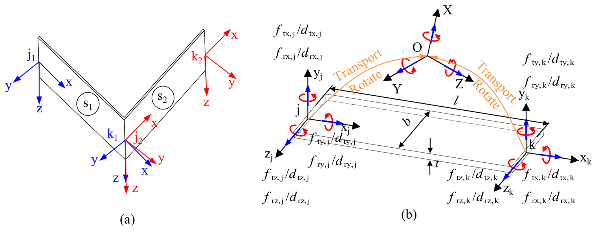
Figure 8 Structural discretization and element analysis: (a) discretization of the folded leaf spring structure and (b) local coordinate system and reference coordinate system of the leaf spring, together with the actuation load and displacement response of the leaf spring.

Figure 9 Compliant spherical joint coordinates.

As shown in Fig. 8b, considering a single leaf spring to be the object of study, its nodes j and k are subjected to driving loads f, producing displacement responses d represented as vectors as follows:

$$\begin{array}{}\text{(10)}& \begin{array}{rl}\mathit{f}=& \left[f_{tx,j}{f}_{ty,j}{f}_{tz,j}{f}_{rx,j}{f}_{ry,j}{f}_{rz,j}{f}_{tx,k}{f}_{ty,k}\right.\\ & {\left.f_{tz,k}{f}_{rx,k}{f}_{ry,k}{f}_{rz,k}\right]}^{\mathrm{T}},\end{array}\end{array}$$

$$\begin{array}{}\text{(11)}& \begin{array}{rl}\mathit{d}=& \left[d_{tx,j}{d}_{ty,j}{d}_{tz,j}{d}_{rx,j}{d}_{ry,j}{d}_{rz,j}{d}_{tx,k}{d}_{ty,k}\right.\\ & {\left.d_{tz,k}{d}_{\mathrm{rx},\mathrm{k}}{d}_{ry,k}{d}_{rz,k}\right]}^{\mathrm{T}},\end{array}\end{array}$$

where f_tx,j denotes the force at node j in the direction of the x_j axis, f_rx,j denotes the torque at node j around the x_j axis, d_tx,j denotes the translational displacement of node j in the x_j direction, and d_rx,j denotes the rotational displacement of node j around the x_j axis, with the rest following similarly. The node-driving loads f and node displacement responses d satisfy the following relationship:

$$\begin{array}{}\text{(12)}& {\mathit{f}}_i={\mathbf{K}}_i\cdot {\mathit{d}}_i,\end{array}$$

where K_i is the stiffness matrix of the element.

The local coordinate systems {J₁} and {K₁} of leaf spring s₁ are rotated to the local coordinate system {J₂}. The driving load ${\mathit{f}}_{\mathrm{1}}^{\mathrm{e}}$ and displacement response ${\mathit{d}}_{\mathrm{1}}^{\mathrm{e}}$ of the s₁ leaf spring in a local coordinate system {J₂} are as follows:

$$\begin{array}{}\text{(13)}& {\mathit{f}}_{\mathrm{1}}^{\mathrm{e}}={\mathbf{R}}^{\mathrm{e}}\cdot {\mathbf{K}}_{\mathrm{1}}\cdot {\mathbf{R}}^{\mathrm{eT}}\cdot {\mathit{d}}_{\mathrm{1}}^{\mathrm{e}},\end{array}$$

where R^e is the rotation matrix as detailed in Eq. (14):

$$\begin{array}{}\text{(14)}& {\mathbf{R}}^{\mathrm{e}}=\left[\begin{array}{cccc}{\mathbf{R}}_{\mathrm{j}}^{\mathrm{e}}& \mathbf{0}& \mathbf{0}& \mathbf{0}\\ \mathbf{0}& {\mathbf{R}}_{\mathrm{j}}^{\mathrm{e}}& \mathbf{0}& \mathbf{0}\\ \mathbf{0}& \mathbf{0}& {\mathbf{R}}_{\mathrm{k}}^{\mathrm{e}}& \mathbf{0}\\ \mathbf{0}& \mathbf{0}& \mathbf{0}& {\mathbf{R}}_{\mathrm{k}}^{\mathrm{e}}\end{array}\right]=\left[\begin{array}{cc}{\mathbf{R}}_{\mathrm{J}}^{\mathrm{e}}& \mathbf{0}\\ \mathbf{0}& {\mathbf{R}}_{\mathrm{K}}^{\mathrm{e}}\end{array}\right],\end{array}$$

where ${\mathbf{R}}_{\mathrm{j}}^{\mathrm{e}}$ and ${\mathbf{R}}_{\mathrm{k}}^{\mathrm{e}}$ are the rotation matrices rotated from the local coordinate system {j₁} and {k₁} to the local coordinate system {j₂}, as detailed in Eqs. (15) and (16):

$$\begin{array}{}\text{(15)}& {\mathbf{R}}_{\mathrm{j}}^{\mathrm{e}}=\left[\begin{array}{ccc}\cos <x_{\mathrm{j}\mathrm{1}},x_{\mathrm{j}\mathrm{2}}>& \cos <y_{\mathrm{j}\mathrm{1}},x_{\mathrm{j}\mathrm{2}}>& \cos <z_{\mathrm{j}\mathrm{1}},x_{\mathrm{j}\mathrm{2}}>\\ \cos <x_{\mathrm{j}\mathrm{1}},y_{\mathrm{j}\mathrm{2}}>& \cos <y_{\mathrm{j}\mathrm{1}},y_{\mathrm{j}\mathrm{2}}>& \cos <z_{\mathrm{j}\mathrm{1}},y_{\mathrm{j}\mathrm{2}}>\\ \cos <x_{\mathrm{j}\mathrm{1}},z_{\mathrm{j}\mathrm{2}}>& \cos <y_{\mathrm{j}\mathrm{1}},z_{\mathrm{j}\mathrm{2}}>& \cos <z_{\mathrm{j}\mathrm{1}},z_{\mathrm{j}\mathrm{2}}>\end{array}\right],\end{array}$$

$$\begin{array}{}\text{(16)}& {\mathbf{R}}_{\mathrm{k}}^{\mathrm{e}}=\left[\begin{array}{ccc}\cos <x_{\mathrm{k}\mathrm{1}},x_{\mathrm{j}\mathrm{2}}>& \cos <y_{\mathrm{k}\mathrm{1}},x_{\mathrm{j}\mathrm{2}}>& \cos <z_{\mathrm{k}\mathrm{1}},x_{\mathrm{j}\mathrm{2}}>\\ \cos <x_{\mathrm{k}\mathrm{1}},y_{\mathrm{j}\mathrm{2}}>& \cos <y_{\mathrm{k}\mathrm{1}},y_{\mathrm{j}\mathrm{2}}>& \cos <z_{\mathrm{k}\mathrm{1}},y_{\mathrm{j}\mathrm{2}}>\\ \cos <x_{\mathrm{k}\mathrm{1}},z_{\mathrm{j}\mathrm{2}}>& \cos <y_{\mathrm{k}\mathrm{1}},z_{\mathrm{j}\mathrm{2}}>& \cos <z_{\mathrm{k}\mathrm{1}},z_{\mathrm{j}\mathrm{2}}>\end{array}\right],\end{array}$$

where < x_j1, x_j2> denotes the angle between the x axis of {j₁} and the x axis of {j₂}, and similarly for the others.

The stiffness matrix ${\mathbf{K}}_{\mathrm{1}}^{\mathrm{e}}$ of the s₁ leaf spring in the local coordinate system {j₂} is given in Eq. (17):

$$\begin{array}{}\text{(17)}& {\mathbf{K}}_{\mathrm{1}}^{\mathrm{e}}={\mathbf{R}}^{\mathrm{e}}\cdot {\mathbf{K}}_{\mathrm{1}}\cdot {\mathbf{R}}^{\mathrm{eT}},\end{array}$$

by partitioning the nodal driving loads ${\mathit{f}}_{\mathrm{1}}^{\mathrm{e}}$ and displacement responses ${\mathit{d}}_{\mathrm{1}}^{\mathrm{e}}$ of the s₁ leaf spring in the local coordinate system {j₂} and those of the s₂ leaf spring, as shown in Eqs. (18) and (19):

$$\begin{array}{}\text{(18)}& {\mathit{f}}_{\mathrm{1}}^{\mathrm{e}}=\left[\begin{array}{c}{\mathit{f}}_{\mathrm{1},\mathrm{j}}^{\mathrm{e}}\\ {\mathit{f}}_{\mathrm{1},\mathrm{k}}^{\mathrm{e}}\end{array}\right]=\left[\begin{array}{cc}{\mathbf{K}}_{\mathrm{1},\mathrm{1}}^{\mathrm{e}}& {\mathbf{K}}_{\mathrm{1},\mathrm{2}}^{\mathrm{e}}\\ {\mathbf{K}}_{\mathrm{1},\mathrm{3}}^{\mathrm{e}}& {\mathbf{K}}_{\mathrm{1},\mathrm{4}}^{\mathrm{e}}\end{array}\right]\cdot \left[\begin{array}{c}{\mathit{d}}_{\mathrm{1},\mathrm{j}}^{\mathrm{e}}\\ {\mathit{d}}_{\mathrm{1},\mathrm{k}}^{\mathrm{e}}\end{array}\right],\end{array}$$

$$\begin{array}{}\text{(19)}& {\mathit{f}}_{\mathrm{2}}=\left[\begin{array}{c}{\mathit{f}}_{\mathrm{2},\mathrm{j}}\\ {\mathit{f}}_{\mathrm{2},\mathrm{k}}\end{array}\right]=\left[\begin{array}{cc}{\mathbf{K}}_{\mathrm{2},\mathrm{1}}& {\mathbf{K}}_{\mathrm{2},\mathrm{2}}\\ {\mathbf{K}}_{\mathrm{2},\mathrm{3}}& {\mathbf{K}}_{\mathrm{2},\mathrm{4}}\end{array}\right]\cdot \left[\begin{array}{c}{\mathit{d}}_{\mathrm{2},\mathrm{j}}\\ {\mathit{d}}_{\mathrm{2},\mathrm{k}}\end{array}\right].\end{array}$$

Considering that k₁ and j₂ are common nodes, the following relationship can be obtained:

$$\begin{array}{}\text{(20)}& {\displaystyle }{\mathit{f}}_{\mathrm{1},\mathrm{k}}^{\mathrm{e}}+{\mathit{f}}_{\mathrm{2},\mathrm{j}}=\mathbf{0},\text{(21)}& {\displaystyle }{\mathit{d}}_{\mathrm{1},\mathrm{k}}^{\mathrm{e}}={\mathit{d}}_{\mathrm{2},\mathrm{j}}.\end{array}$$

Figure 10 Discretization of the compliant translational joint.

Combining Eqs. (18)–(21) yields (Eq. 22)

$$\begin{array}{}\text{(22)}& {\mathit{d}}_{\mathrm{2},\mathrm{j}}=-{\left({\mathbf{K}}_{\mathrm{1},\mathrm{4}}^{\mathrm{e}}+{\mathbf{K}}_{\mathrm{2},\mathrm{1}}\right)}^{-\mathrm{1}}\cdot ({\mathbf{K}}_{\mathrm{1},\mathrm{3}}^{\mathrm{e}}\cdot {\mathit{d}}_{\mathrm{1},\mathrm{j}}^{\mathrm{e}}+{\mathbf{K}}_{\mathrm{2},\mathrm{2}}\cdot {\mathit{d}}_{\mathrm{2},\mathrm{k}}).\end{array}$$

Eqs. (13) and (14) provide the basis for deriving Eqs. (23) and (24):

$$\begin{array}{}\text{(23)}& {\mathit{d}}_{\mathrm{1},\mathrm{j}}={\mathbf{R}}_{\mathrm{J}}^{\mathrm{eT}}\cdot {\mathit{d}}_{\mathrm{1},\mathrm{j}}^{\mathrm{e}},\end{array}$$

$$\begin{array}{}\text{(24)}& {\mathit{d}}_{\mathrm{1},\mathrm{k}}={\mathbf{R}}_{\mathrm{K}}^{\mathrm{eT}}\cdot {\mathit{d}}_{\mathrm{1},\mathrm{k}}^{\mathrm{e}}.\end{array}$$

Combining Eqs. (21)–(24) leads to Eq. (15):

$$\begin{array}{}\text{(25)}& \begin{array}{rl}& {\mathit{f}}_{\mathrm{1},\mathrm{j}}=\left({\mathbf{K}}_{\mathrm{1},\mathrm{1}}-{\mathbf{K}}_{\mathrm{1},\mathrm{2}}\cdot {\mathbf{R}}_{\mathrm{K}}^{\mathrm{eT}}\cdot {\left({\mathbf{K}}_{\mathrm{1},\mathrm{4}}^{\mathrm{e}}+{\mathbf{K}}_{\mathrm{2},\mathrm{1}}\right)}^{-\mathrm{1}}\cdot {\mathbf{K}}_{\mathrm{1},\mathrm{3}}^{\mathrm{e}}\cdot {\mathbf{R}}_{\mathrm{J}}^{\mathrm{e}}\right),\\ & \cdot {\mathit{d}}_{\mathrm{1},\mathrm{j}}-{\mathbf{K}}_{\mathrm{1},\mathrm{2}}\cdot {\mathbf{R}}_{\mathrm{K}}^{\mathrm{eT}}\cdot {\left({\mathbf{K}}_{\mathrm{1},\mathrm{4}}^{\mathrm{e}}+{\mathbf{K}}_{\mathrm{2},\mathrm{1}}\right)}^{-\mathrm{1}}\cdot {\mathbf{K}}_{\mathrm{2},\mathrm{2}}\cdot {\mathit{d}}_{\mathrm{2},\mathrm{k}}.\end{array}\end{array}$$

Combining Eqs. (19) and (22) leads to Eq. (26):

$$\begin{array}{}\text{(26)}& \begin{array}{rl}& {\mathit{f}}_{\mathrm{2},\mathrm{k}}=-{\mathbf{K}}_{\mathrm{2},\mathrm{3}}\cdot {\left({\mathbf{K}}_{\mathrm{1},\mathrm{4}}^{\mathrm{e}}+{\mathbf{K}}_{\mathrm{2},\mathrm{1}}\right)}^{-\mathrm{1}}{\mathbf{K}}_{\mathrm{1},\mathrm{3}}^{\mathrm{e}}\cdot {\mathbf{R}}_{\mathrm{J}}^{\mathrm{e}}\cdot {\mathit{d}}_{\mathrm{1},\mathrm{j}}\\ & +\left({\mathbf{K}}_{\mathrm{2},\mathrm{4}}-{\mathbf{K}}_{\mathrm{2},\mathrm{3}}\cdot {\left({\mathbf{K}}_{\mathrm{1},\mathrm{4}}^{\mathrm{e}}+{\mathbf{K}}_{\mathrm{2},\mathrm{1}}\right)}^{-\mathrm{1}}\cdot {\mathbf{K}}_{\mathrm{2},\mathrm{2}}\right.)\cdot {\mathit{d}}_{\mathrm{2},\mathrm{k}}.\end{array}\end{array}$$

Therefore, the relationship between the driving loads and displacement responses of the single folded leaf spring j₁ node and k₂ node can be obtained as follows:

$$\begin{array}{}\text{(27)}& \begin{array}{rl}& \left[\begin{array}{l}{\mathit{f}}_{\mathrm{1},\mathrm{j}}\\ {\mathit{f}}_{\mathrm{2},\mathrm{k}}\end{array}\right]\\ & =\left[\begin{array}{ll}& {\mathbf{K}}_{\mathrm{1},\mathrm{1}}-{\mathbf{K}}_{\mathrm{1},\mathrm{2}}\cdot {\mathbf{R}}_{\mathrm{K}}^{\mathrm{eT}}\cdot {\left({\mathbf{K}}_{\mathrm{1},\mathrm{4}}^{\mathrm{e}}+{\mathbf{K}}_{\mathrm{2},\mathrm{1}}\right)}^{-\mathrm{1}}\\ & \cdot {\mathbf{K}}_{\mathrm{1},\mathrm{3}}^{\mathrm{e}}\cdot {\mathbf{R}}_{\mathrm{J}}^{\mathrm{e}}-{\mathbf{K}}_{\mathrm{1},\mathrm{2}}\cdot {\mathbf{R}}_{\mathrm{K}}^{\mathrm{eT}}\cdot {\left({\mathbf{K}}_{\mathrm{1},\mathrm{4}}^{\mathrm{e}}+{\mathbf{K}}_{\mathrm{2},\mathrm{1}}\right)}^{-\mathrm{1}}\\ & \cdot {\mathbf{K}}_{\mathrm{2},\mathrm{2}}-{\mathbf{K}}_{\mathrm{2},\mathrm{3}}\cdot {\left({\mathbf{K}}_{\mathrm{1},\mathrm{4}}^{\mathrm{e}}+{\mathbf{K}}_{\mathrm{2},\mathrm{1}}\right)}^{-\mathrm{1}}\\ & \cdot {\mathbf{K}}_{\mathrm{1},\mathrm{3}}^{\mathrm{e}}\cdot {\mathbf{R}}_{\mathrm{J}}^{\mathrm{e}}-{\mathbf{K}}_{\mathrm{2},\mathrm{3}}\cdot {\left({\mathbf{K}}_{\mathrm{1},\mathrm{4}}^{\mathrm{e}}+{\mathbf{K}}_{\mathrm{2},\mathrm{1}}\right)}^{-\mathrm{1}}\\ & \cdot {\mathbf{K}}_{\mathrm{2},\mathrm{2}}+{\mathbf{K}}_{\mathrm{2},\mathrm{4}}\end{array}\right]\\ & \cdot \left[\begin{array}{l}{\mathit{d}}_{\mathrm{1},\mathrm{j}}\\ {\mathit{d}}_{\mathrm{2},\mathrm{k}}\end{array}\right]=\left[\begin{array}{cc}{\mathbf{K}}_{\mathrm{1}}^{\mathrm{a}}& {\mathbf{K}}_{\mathrm{2}}^{\mathrm{a}}\\ {\mathbf{K}}_{\mathrm{3}}^{\mathrm{a}}& {\mathbf{K}}_{\mathrm{4}}^{\mathrm{a}}\end{array}\right]\cdot \left[\begin{array}{l}{\mathit{d}}_{\mathrm{1},\mathrm{j}}\\ {\mathit{d}}_{\mathrm{2},\mathrm{k}}\end{array}\right].\end{array}\end{array}$$

For the mth folded leaf spring, assigning node j₁ as j and node k₂ as k leads to the relationship shown in Eq. (28):

$$\begin{array}{}\text{(28)}& \left[\begin{array}{l}{\mathit{f}}_{m,\mathrm{j}}^{\mathrm{a}}\\ {\mathit{f}}_{m,\mathrm{k}}^{\mathrm{a}}\end{array}\right]=\left[\begin{array}{cc}{\mathbf{K}}_{m,\mathrm{1}}^{\mathrm{a}}& {\mathbf{K}}_{m,\mathrm{2}}^{\mathrm{a}}\\ {\mathbf{K}}_{m,\mathrm{3}}^{\mathrm{a}}& {\mathbf{K}}_{m,\mathrm{4}}^{\mathrm{a}}\end{array}\right]\cdot \left[\begin{array}{l}{\mathit{d}}_{m,\mathrm{j}}^{\mathrm{a}}\\ {\mathit{d}}_{m,\mathrm{k}}^{\mathrm{a}}\end{array}\right].\end{array}$$

Figure 11 A flowchart for FEM numerical analysis.

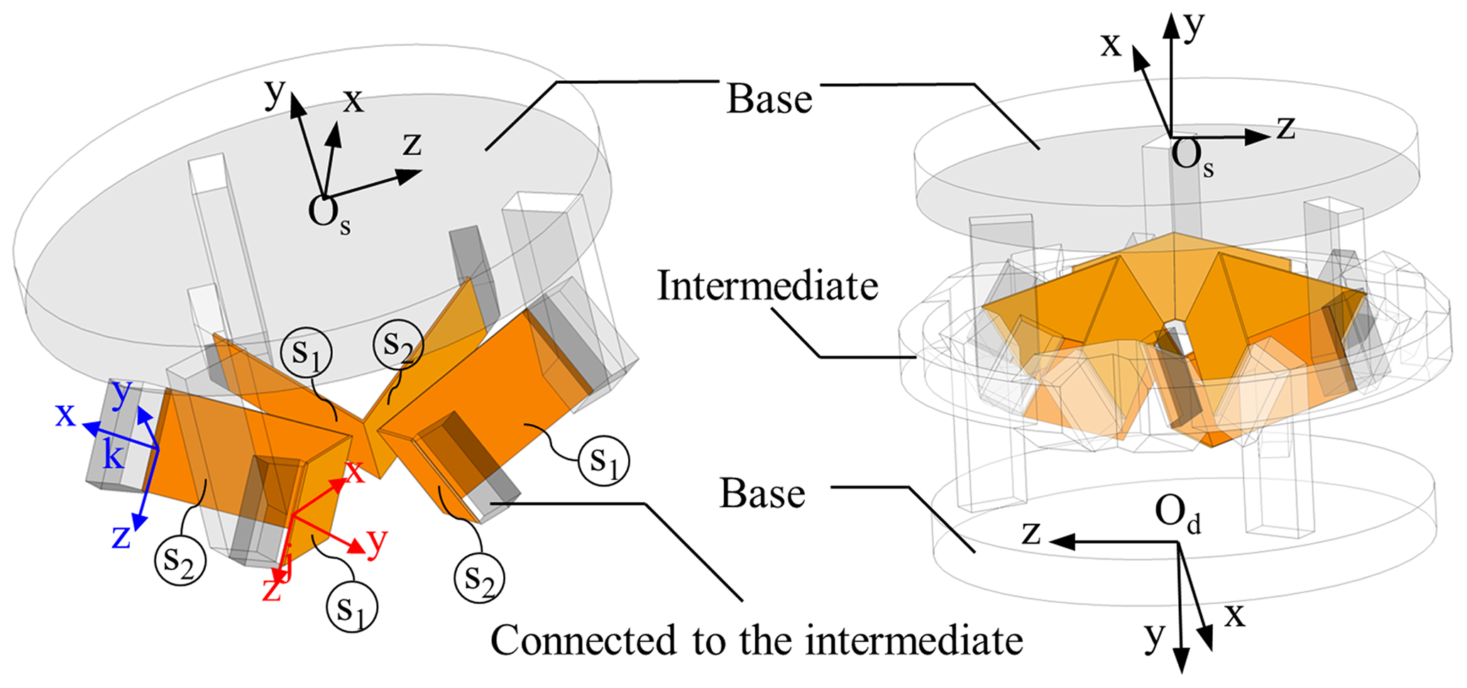
A reference coordinate system {O_s} is established at the center of the upper surface of the compliant spherical joint. One end of the folded leaf spring is attached to the base and designated as the j end, while the opposite end is connected to the intermediate body and referred to as the k end. When the driving load F_s is applied at the origin of the coordinate system {O_s}, the resultant displacement response is d_s. At this point, for the mth folded leaf spring, the displacement responses ${\mathit{d}}_{m,\mathrm{j}}^{\mathrm{a}}$ at the j node can be expressed as

$$\begin{array}{}\text{(29)}& {\mathit{d}}_{m,\mathrm{j}}^{\mathrm{a}}={\mathbf{T}}_{\mathrm{s},m}\cdot {\mathbf{R}}_{\mathrm{s},m}\cdot {\mathit{d}}_{\mathrm{s}},\end{array}$$

where T_s,m and R_s,m are the coordinate shift matrix and rotation matrix, respectively, as detailed in Eqs. (30) and (31):

$$\begin{array}{}\text{(30)}& {\mathbf{T}}_{\mathrm{s},m}=\left[\begin{array}{cccccc}\mathrm{1}& \mathrm{0}& \mathrm{0}& \mathrm{0}& -z_{\mathrm{s},m}& y_{\mathrm{s},m}\\ \mathrm{0}& \mathrm{1}& \mathrm{0}& z_{\mathrm{s},m}& \mathrm{0}& -x_{\mathrm{s},m}\\ \mathrm{0}& \mathrm{0}& \mathrm{1}& -y_{\mathrm{s},m}& x_{\mathrm{s},m}& \mathrm{0}\\ \mathrm{0}& \mathrm{0}& \mathrm{0}& \mathrm{1}& \mathrm{0}& \mathrm{0}\\ \mathrm{0}& \mathrm{0}& \mathrm{0}& \mathrm{0}& \mathrm{1}& \mathrm{0}\\ \mathrm{0}& \mathrm{0}& \mathrm{0}& \mathrm{0}& \mathrm{0}& \mathrm{1}\end{array}\right],\end{array}$$

$$\begin{array}{}\text{(31)}& {\mathbf{R}}_{\mathrm{s},m}=\left[\begin{array}{cccccc}<x_{\mathrm{j}}^m,x_{\mathrm{s}}>& <x_{\mathrm{j}}^m,y_{\mathrm{s}}>& <x_{\mathrm{j}}^m,z_{\mathrm{s}}>& \mathrm{0}& \mathrm{0}& \mathrm{0}\\ <y_{\mathrm{j}}^m,x_{\mathrm{s}}>& <y_{\mathrm{j}}^m,y_{\mathrm{s}}>& <y_{\mathrm{j}}^m,z_{\mathrm{s}}>& \mathrm{0}& \mathrm{0}& \mathrm{0}\\ <z_{\mathrm{j}}^m,x_{\mathrm{s}}>& <z_{\mathrm{j}}^m,y_{\mathrm{s}}>& <z_{\mathrm{j}}^m,z_{\mathrm{s}}>& \mathrm{0}& \mathrm{0}& \mathrm{0}\\ \mathrm{0}& \mathrm{0}& \mathrm{0}& <x_{\mathrm{j}}^m,x_{\mathrm{s}}>& <x_{\mathrm{j}}^m,y_{\mathrm{s}}>& <x_{\mathrm{j}}^m,z_{\mathrm{s}}>\\ \mathrm{0}& \mathrm{0}& \mathrm{0}& <y_{\mathrm{j}}^m,x_{\mathrm{s}}>& <y_{\mathrm{j}}^m,y_{\mathrm{s}}>& <y_{\mathrm{j}}^m,z_{\mathrm{s}}>\\ \mathrm{0}& \mathrm{0}& \mathrm{0}& <z_{\mathrm{j}}^m,x_{\mathrm{s}}>& <z_{\mathrm{j}}^m,y_{\mathrm{s}}>& <z_{\mathrm{j}}^m,z_{\mathrm{s}}>\end{array}\right],\end{array}$$

where (x_s,m, y_s,m, z_s,m) represents the coordinates of the origin of the local coordinate system {j} of the mth folded leaf spring in the reference coordinate system {O_s} and $<x_{\mathrm{j}}^m{x}_{\mathrm{s}}>$ denotes the angle between the x axis of the local coordinate system {j} of the mth folded leaf spring and the x axis of the reference coordinate system {O_s}, with the same applying to the others.

Assuming that the intermediate body of the compliant spherical joint is fixed, the displacement of the k node of the mth folded leaf spring becomes 0. Substituting Eq. (29) into Eq. (28) and setting ${\mathit{d}}_{m,k}^{\mathrm{a}}=\mathrm{0}$ yields Eq. (32):

$$\begin{array}{}\text{(32)}& {\mathit{f}}_{m,\mathrm{j}}^{\mathrm{a}}={\mathbf{K}}_{m,\mathrm{1}}^{\mathrm{a}}\cdot {\mathbf{T}}_{\mathrm{s},m}\cdot {\mathbf{R}}_{\mathrm{s},m}\cdot {\mathit{d}}_{\mathrm{s}}.\end{array}$$

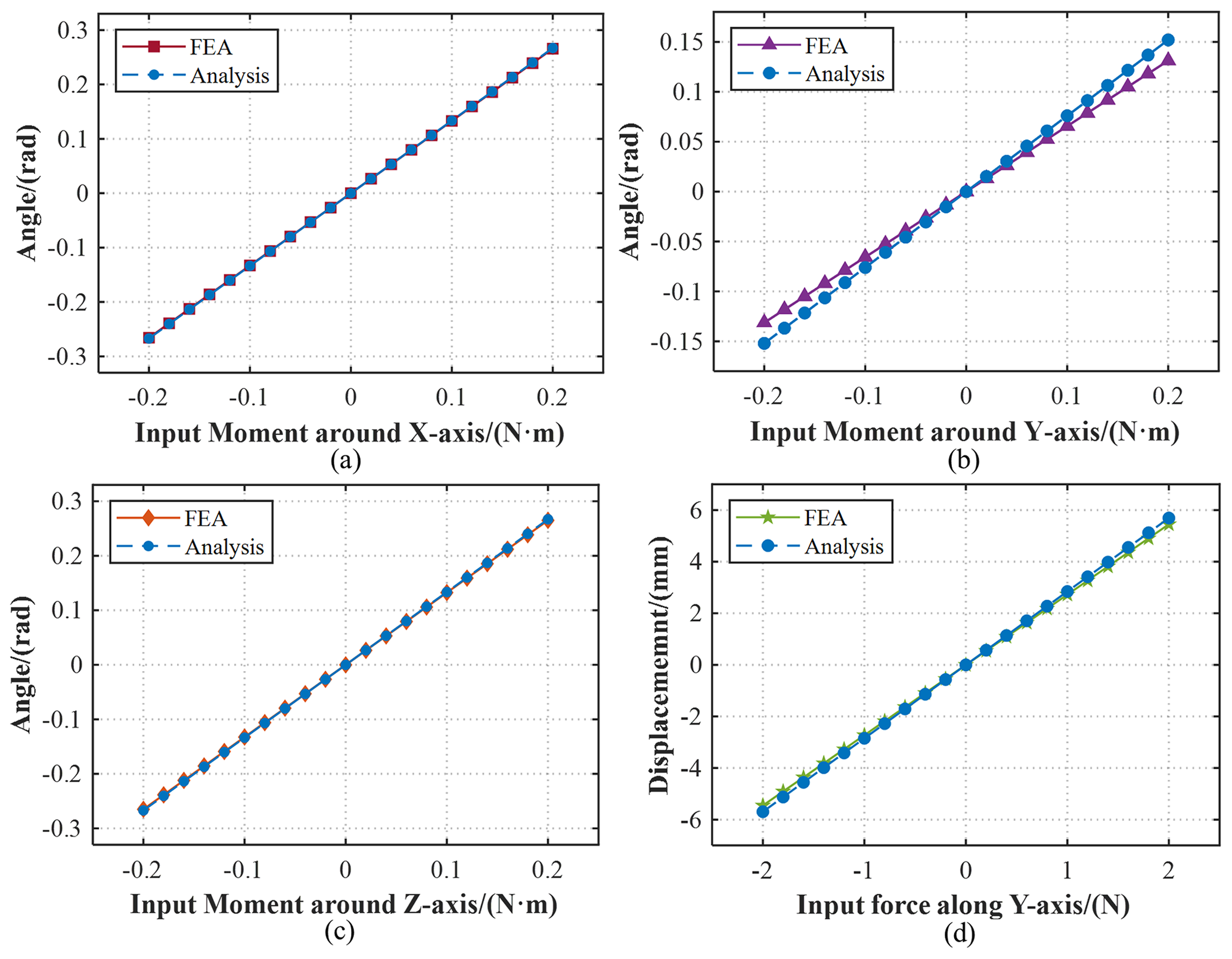
Figure 12 Relationship between input load and output displacement: (a) the moment around the x axis is applied to the compliant spherical joint. (b) The moment around the y axis is applied to the compliant spherical joint. (c) The moment around the z axis is applied to the compliant spherical joint. (d) The force around the y axis is applied to the compliant translational joint.

Transforming the loads at node j of the mth folded leaf spring to the reference coordinate system {O_s} gives Eq. (33):

$$\begin{array}{}\text{(33)}& {\mathit{f}}_m={\mathbf{R}}_{\mathrm{o},m}\cdot {\mathbf{T}}_{\mathrm{o},m}\cdot {\mathit{f}}_{m,\mathrm{j}}^{\mathrm{a}},\end{array}$$

where T_o,m and R_o,m are the coordinate translation and rotation matrices as detailed in Eqs. (34) and (35):

$$\begin{array}{}\text{(34)}& {\displaystyle }{\mathbf{T}}_{\mathrm{o},m}={\mathbf{T}}_{\mathrm{s},m}^{\mathrm{T}},\text{(35)}& {\displaystyle }{\mathbf{R}}_{\mathrm{o},m}={\mathbf{R}}_{\mathrm{s},m}^{\mathrm{T}}.\end{array}$$

Given that there are three folded leaf springs connected to the base, as depicted in Fig. 9, Eq. (36) can be established:

$$\begin{array}{}\text{(36)}& {\mathit{F}}_{\mathrm{s}}=\sum _{m=\mathrm{1}}^{\mathrm{3}}{\mathit{f}}_m.\end{array}$$

Combining Eqs. (32) to (36) leads to Eq. (37):

$$\begin{array}{}\text{(37)}& {\mathit{F}}_{\mathrm{s}}={\mathbf{K}}_{\mathrm{s}}\cdot {\mathit{d}}_{\mathrm{s}}.\end{array}$$

Since the upper and lower folded leaf springs of the compliant spherical joint are symmetrical about the plane perpendicular to the rotation axis and each set of folded leaf springs contributes half of the motion, the overall displacement responses d_r of the compliant spherical joint are as follows:

$$\begin{array}{}\text{(38)}& {\mathit{d}}_{\mathrm{r}}=\mathrm{2}{\mathit{d}}_{\mathrm{s}}.\end{array}$$

Table 1 Parameters of the compliant mechanism.

4.2 Kinetostatic modeling of the compliant translational joint

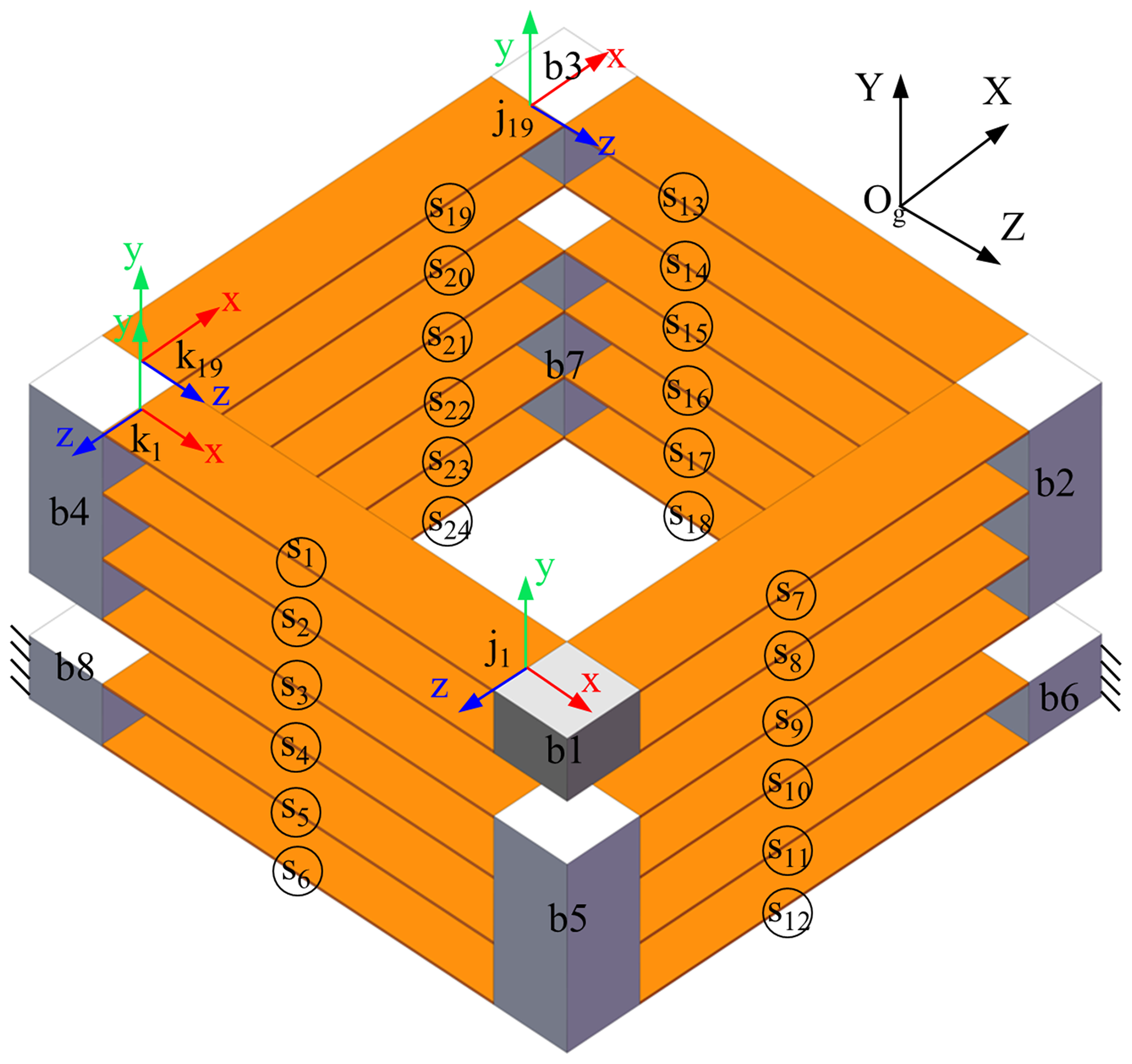
The compliant translational joint is discretized into compliant leaf springs and rigid bodies, as shown in Fig. 10. The rigid bodies are numbered b₁, b₂, ..., b₈, and the compliant leaf springs are labeled s₁, s₂, ..., s₂₄. The end nodes of each leaf spring s_n are defined as j_n and k_n, with the local coordinate systems {j_n} and {k_n} established at these nodes. The local coordinate system directions for s₁, s₂, s₃, s₄, s₅, s₆, s₁₃, s₁₄, s₁₅, s₁₆, s₁₇ and s₁₈ are consistent, as are those for s₇, s₈, s_9, s₁₀, s₁₁, s₁₂, s₁₉, s₂₀, s₂₁, s₂₂, s₂₃ and s₂₄. Following a similar methodology to that used in the kinetostatic modeling of the compliant spherical joint, element analysis is conducted post discretization, though the details are not reiterated here. Since compliant leaf springs are connected to rigid bodies, nodes j_n and k_n of s_n are moved to the centroids J_n and K_n of the rigid bodies to form the extended compliant leaf spring S_n, turning the rigid body into a concentrated mass before transforming it to the global coordinate system {O_g}.

The relationship between the driving loads ${\mathbf{F}}_n^{\mathrm{g}}$ of the leaf spring S_n in the global coordinate system {O_g} and the nodal displacement responses ${\mathbf{D}}_n^{\mathrm{g}}$ is

$$\begin{array}{}\text{(39)}& {\mathbf{F}}_n^{\mathrm{g}}={\mathbf{R}}_n^{\mathrm{g}}\cdot {\mathbf{T}}_n^{\mathrm{g}}\cdot {\mathbf{K}}_n^{\mathrm{g}}\cdot {\mathbf{T}}_n^{\mathrm{gT}}\cdot {\mathbf{R}}_n^{\mathrm{gT}}\cdot {\mathbf{D}}_n^{\mathrm{g}},\end{array}$$

where ${\mathbf{T}}_n^{\mathrm{g}}$ and ${\mathbf{R}}_n^{\mathrm{g}}$ are the coordinate translation and rotation matrices, respectively, defined as

$$\begin{array}{}\text{(40)}& {\mathbf{T}}_n^{\mathrm{g}}=\left[\begin{array}{cc}{\mathbf{T}}_{n,\mathrm{j}}^{\mathrm{g}}& \\ & {\mathbf{T}}_{n,\mathrm{k}}^{\mathrm{g}}\end{array}\right],\end{array}$$

$$\begin{array}{}\text{(41)}& {\mathbf{R}}_n^{\mathrm{g}}=\left[\begin{array}{cccc}{\mathbf{R}}_{n,\mathrm{j}}^{\mathrm{g}}& \mathbf{0}& \mathbf{0}& \mathbf{0}\\ \mathbf{0}& {\mathbf{R}}_{n,\mathrm{j}}^{\mathrm{g}}& \mathbf{0}& \mathbf{0}\\ \mathbf{0}& \mathbf{0}& {\mathbf{R}}_{n,\mathrm{k}}^{\mathrm{g}}& \mathbf{0}\\ \mathbf{0}& \mathbf{0}& \mathbf{0}& {\mathbf{R}}_{n,\mathrm{k}}^{\mathrm{g}}\end{array}\right],\end{array}$$

with ${\mathbf{T}}_{n,\mathrm{j}}^{\mathrm{g}}$ and ${\mathbf{T}}_{n,\mathrm{k}}^{\mathrm{g}}$ representing the coordinate translation matrices as shown in Eqs. (42) and (43) and ${\mathbf{R}}_{n,\mathrm{j}}^{\mathrm{g}}$ and ${\mathbf{R}}_{n,\mathrm{k}}^{\mathrm{g}}$ representing the coordinate rotation matrices as shown in Eqs. (44) and (45):

$$\begin{array}{}\text{(42)}& {\mathbf{T}}_{n,\mathrm{j}}^{\mathrm{g}}=\left[\begin{array}{cccccc}\mathrm{1}& \mathrm{0}& \mathrm{0}& \mathrm{0}& \mathrm{0}& \mathrm{0}\\ \mathrm{0}& \mathrm{1}& \mathrm{0}& \mathrm{0}& \mathrm{0}& \mathrm{0}\\ \mathrm{0}& \mathrm{0}& \mathrm{1}& \mathrm{0}& \mathrm{0}& \mathrm{0}\\ \mathrm{0}& z_{n,\mathrm{j}}& -y_{n,\mathrm{j}}& \mathrm{1}& \mathrm{0}& \mathrm{0}\\ -z_{n,\mathrm{j}}& \mathrm{0}& x_{n,\mathrm{j}}& \mathrm{0}& \mathrm{1}& \mathrm{0}\\ y_{n,\mathrm{j}}& -x_{n,\mathrm{j}}& \mathrm{0}& \mathrm{0}& \mathrm{0}& \mathrm{1}\end{array}\right],\end{array}$$

$$\begin{array}{}\text{(43)}& {\mathbf{T}}_{n,\mathrm{k}}^{\mathrm{g}}=\left[\begin{array}{cccccc}\mathrm{1}& \mathrm{0}& \mathrm{0}& \mathrm{0}& \mathrm{0}& \mathrm{0}\\ \mathrm{0}& \mathrm{1}& \mathrm{0}& \mathrm{0}& \mathrm{0}& \mathrm{0}\\ \mathrm{0}& \mathrm{0}& \mathrm{1}& \mathrm{0}& \mathrm{0}& \mathrm{0}\\ \mathrm{0}& z_{n,\mathrm{k}}& -y_{n,\mathrm{k}}& \mathrm{1}& \mathrm{0}& \mathrm{0}\\ -z_{n,\mathrm{k}}& \mathrm{0}& x_{n,\mathrm{k}}& \mathrm{0}& \mathrm{1}& \mathrm{0}\\ y_{n,\mathrm{k}}& -x_{n,\mathrm{k}}& \mathrm{0}& \mathrm{0}& \mathrm{0}& \mathrm{1}\end{array}\right],\end{array}$$

$$\begin{array}{}\text{(44)}& {\mathbf{R}}_{n,\mathrm{j}}^{\mathrm{g}}=\left[\begin{array}{c}\cos <x_{\mathrm{j}}^n,x_{\mathrm{g}}>\cos <y_{\mathrm{j}}^n,x_{\mathrm{g}}>\cos <z_{\mathrm{j}}^n,x_{\mathrm{g}}>\\ \cos <x_{\mathrm{j}}^n,y_{\mathrm{g}}>\cos <y_{\mathrm{j}}^n,y_{\mathrm{g}}>\cos <z_{\mathrm{j}}^n,y_{\mathrm{g}}>\\ \cos <x_{\mathrm{j}}^n,z_{\mathrm{g}}>\cos <y_{\mathrm{j}}^n,z_{\mathrm{g}}>\cos <z_{\mathrm{j}}^n,z_{\mathrm{g}}>\end{array}\right],\end{array}$$

$$\begin{array}{}\text{(45)}& {\mathbf{R}}_{n,\mathrm{k}}^{\mathrm{g}}=\left[\begin{array}{c}\cos <x_{\mathrm{k}}^n,x_{\mathrm{g}}>\cos <y_{\mathrm{k}}^n,x_{\mathrm{g}}>\cos <z_{\mathrm{k}}^n,x_{\mathrm{g}}>\\ \cos <x_{\mathrm{k}}^n,y_{\mathrm{g}}>\cos <y_{\mathrm{k}}^n,y_{\mathrm{g}}>\cos <z_{\mathrm{k}}^n,y_{\mathrm{g}}>\\ \cos <x_{\mathrm{k}}^n,z_{\mathrm{g}}>\cos <y_{\mathrm{k}}^n,z_{\mathrm{g}}>\cos <z_{\mathrm{k}}^n,z_{\mathrm{g}}>\end{array}\right],\end{array}$$

where $<x_{\mathrm{j}}^n{x}_{\mathrm{g}}>$ denotes the angle between the x axis of the local coordinate system {j_n} and the x axis of the global coordinate system {O_g}, and similarly for the others.

Consequently, the stiffness matrix ${\mathbf{K}}_n^{\mathrm{g}}$ of the leaf spring s_n in the global coordinate system is represented as

$$\begin{array}{}\text{(46)}& {\mathbf{K}}_n^{\mathrm{g}}={\mathbf{R}}_n^{\mathrm{g}}\cdot {\mathbf{T}}_n^{\mathrm{g}}\cdot {\mathbf{K}}_n\cdot {\mathbf{T}}_n^{\mathrm{gT}}\cdot {\mathbf{R}}_n^{\mathrm{gT}}.\end{array}$$

Similarly, by partitioning the nodal loads and displacements of s_n in the global coordinate system, we obtain

$$\begin{array}{}\text{(47)}& {\mathbf{F}}_n^{\mathrm{g}}=\left[\begin{array}{l}{\mathbf{F}}_{n,\mathrm{J}}^{\mathrm{g}}\\ {\mathbf{F}}_{n,\mathrm{K}}^{\mathrm{g}}\end{array}\right]=\left[\begin{array}{cc}{\mathbf{K}}_{n,\mathrm{1}}^{\mathrm{g}}& {\mathbf{K}}_{n,\mathrm{2}}^{\mathrm{g}}\\ {\mathbf{K}}_{n,\mathrm{3}}^{\mathrm{g}}& {\mathbf{K}}_{n,\mathrm{4}}^{\mathrm{g}}\end{array}\right]\cdot \left[\begin{array}{l}{\mathbf{D}}_{n,\mathrm{J}}^{\mathrm{g}}\\ {\mathbf{D}}_{n,\mathrm{K}}^{\mathrm{g}}\end{array}\right].\end{array}$$

${\mathbf{F}}_{n,\mathrm{J}}^{\mathrm{g}}$ and ${\mathbf{F}}_{n,\mathrm{K}}^{\mathrm{g}}$ are the nodal loads. ${\mathbf{D}}_{n,\mathrm{J}}^{\mathrm{g}}$ and ${\mathbf{D}}_{n,\mathrm{K}}^{\mathrm{g}}$ are the nodal displacements. ${\mathbf{K}}_{n,\mathrm{1}}^{\mathrm{g}}$, ${\mathbf{K}}_{n,\mathrm{2}}^{\mathrm{g}}$, ${\mathbf{K}}_{n,\mathrm{3}}^{\mathrm{g}}$ and ${\mathbf{K}}_{n,\mathrm{4}}^{\mathrm{g}}$ are the partitioned matrices of the stiffness matrix ${\mathbf{K}}_n^{\mathrm{g}}$ in the global coordinate system.

For each rigid body b_ω,

$$\begin{array}{}\text{(48)}& \sum _{n=\mathrm{1}}^N{\mathit{F}}_{n,\mathrm{J}/\mathrm{K}}^{\mathrm{g}}={\mathit{\zeta }}_{\mathit{\omega }},\end{array}$$

where N is the total number of compliant leaf springs connected to b_w and ζ_w is the external force on node w of the rigid body.

Selecting each rigid body node of the compliant structure for study, we establish the equation set.

$$\begin{array}{}\text{(49)}& \left[\begin{array}{l}{\mathit{\zeta }}_{\mathrm{1}}\\ {\mathit{\zeta }}_{\mathrm{2}}\\ {\mathit{\zeta }}_{\mathrm{3}}\\ {\mathit{\zeta }}_{\mathrm{4}}\\ {\mathit{\zeta }}_{\mathrm{5}}\\ {\mathit{\zeta }}_{\mathrm{7}}\end{array}\right]=\left[\begin{array}{cccccc}{\mathbf{\Gamma }}_{\mathrm{1}}& {\mathbf{\Gamma }}_{\mathrm{8}}& & {\mathbf{\Gamma }}_{\mathrm{10}}& & \\ {\mathbf{\Gamma }}_{\mathrm{9}}& {\mathbf{\Gamma }}_{\mathrm{2}}& {\mathbf{\Gamma }}_{\mathrm{11}}& & {\mathbf{\Gamma }}_{\mathrm{14}}& {\mathbf{\Gamma }}_{\mathrm{18}}\\ & {\mathbf{\Gamma }}_{\mathrm{12}}& {\mathbf{\Gamma }}_{\mathrm{3}}& {\mathbf{\Gamma }}_{\mathrm{15}}& & \\ {\mathbf{\Gamma }}_{\mathrm{13}}& & {\mathbf{\Gamma }}_{\mathrm{16}}& {\mathbf{\Gamma }}_{\mathrm{4}}& {\mathbf{\Gamma }}_{\mathrm{20}}& {\mathbf{\Gamma }}_{\mathrm{22}}\\ & {\mathbf{\Gamma }}_{\mathrm{17}}& & {\mathbf{\Gamma }}_{\mathrm{21}}& {\mathbf{\Gamma }}_{\mathrm{5}}& \\ & {\mathbf{\Gamma }}_{\mathrm{19}}& & {\mathbf{\Gamma }}_{\mathrm{23}}& & {\mathbf{\Gamma }}_{\mathrm{7}}\end{array}\right]\cdot \left[\begin{array}{l}{\mathit{\xi }}_{\mathrm{1}}\\ {\mathit{\xi }}_{\mathrm{2}}\\ {\mathit{\xi }}_{\mathrm{3}}\\ {\mathit{\xi }}_{\mathrm{4}}\\ {\mathit{\xi }}_{\mathrm{5}}\\ {\mathit{\xi }}_{\mathrm{7}}\end{array}\right]\end{array}$$

ξ_w is the nodal displacement of w. The matrix elements Γ_u are as follows.

$$\begin{array}{rl}& {\mathbf{\Gamma }}_{\mathrm{1}}={\mathbf{K}}_{\mathrm{1},\mathrm{1}}^{\mathrm{g}}+{\mathbf{K}}_{\mathrm{2},\mathrm{1}}^{\mathrm{g}}+{\mathbf{K}}_{\mathrm{7},\mathrm{4}}^{\mathrm{g}}+{\mathbf{K}}_{\mathrm{8},\mathrm{4}}^{\mathrm{g}}\\ & {\mathbf{\Gamma }}_{\mathrm{2}}={\mathbf{K}}_{\mathrm{7},\mathrm{1}}^{\mathrm{g}}+{\mathbf{K}}_{\mathrm{8},\mathrm{1}}^{\mathrm{g}}+{\mathbf{K}}_{\mathrm{9},\mathrm{1}}^{\mathrm{g}}+{\mathbf{K}}_{\mathrm{10},\mathrm{1}}^{\mathrm{g}}\\ & +{\mathbf{K}}_{\mathrm{13},\mathrm{1}}^{\mathrm{g}}+{\mathbf{K}}_{\mathrm{14},\mathrm{1}}^{\mathrm{g}}+{\mathbf{K}}_{\mathrm{15},\mathrm{1}}^{\mathrm{g}}+{\mathbf{K}}_{\mathrm{16},\mathrm{1}}^{\mathrm{g}}\\ & {\mathbf{\Gamma }}_{\mathrm{3}}={\mathbf{K}}_{\mathrm{13},\mathrm{4}}^{\mathrm{g}}+{\mathbf{K}}_{\mathrm{14},\mathrm{4}}^{\mathrm{g}}+{\mathbf{K}}_{\mathrm{19},\mathrm{1}}^{\mathrm{g}}+{\mathbf{K}}_{\mathrm{20},\mathrm{1}}^{\mathrm{g}}\\ & {\mathbf{\Gamma }}_{\mathrm{4}}={\mathbf{K}}_{\mathrm{1},\mathrm{4}}^{\mathrm{g}}+{\mathbf{K}}_{\mathrm{2},\mathrm{4}}^{\mathrm{g}}+{\mathbf{K}}_{\mathrm{3},\mathrm{4}}^{\mathrm{g}}+{\mathbf{K}}_{\mathrm{4},\mathrm{4}}^{\mathrm{g}}\\ & +{\mathbf{K}}_{\mathrm{19},\mathrm{4}}^{\mathrm{g}}+{\mathbf{K}}_{\mathrm{20},\mathrm{4}}^{\mathrm{g}}+{\mathbf{K}}_{\mathrm{21},\mathrm{4}}^{\mathrm{g}}+{\mathbf{K}}_{\mathrm{22},\mathrm{4}}^{\mathrm{g}}\\ & {\mathbf{\Gamma }}_{\mathrm{5}}={\mathbf{K}}_{\mathrm{3},\mathrm{1}}^{\mathrm{g}}+{\mathbf{K}}_{\mathrm{4},\mathrm{1}}^{\mathrm{g}}+{\mathbf{K}}_{\mathrm{5},\mathrm{1}}^{\mathrm{g}}+{\mathbf{K}}_{\mathrm{6},\mathrm{1}}^{\mathrm{g}}\\ & +{\mathbf{K}}_{\mathrm{9},\mathrm{4}}^{\mathrm{g}}+{\mathbf{K}}_{\mathrm{10},\mathrm{4}}^{\mathrm{g}}+{\mathbf{K}}_{\mathrm{11},\mathrm{4}}^{\mathrm{g}}+{\mathbf{K}}_{\mathrm{12},\mathrm{4}}^{\mathrm{g}}\\ & {\mathbf{\Gamma }}_{\mathrm{7}}={\mathbf{K}}_{\mathrm{15},\mathrm{4}}^{\mathrm{g}}+{\mathbf{K}}_{\mathrm{16},\mathrm{4}}^{\mathrm{g}}+{\mathbf{K}}_{\mathrm{17},\mathrm{4}}^{\mathrm{g}}+{\mathbf{K}}_{\mathrm{18},\mathrm{4}}^{\mathrm{g}}\\ & +{\mathbf{K}}_{\mathrm{21},\mathrm{1}}^{\mathrm{g}}+{\mathbf{K}}_{\mathrm{22},\mathrm{1}}^{\mathrm{g}}+{\mathbf{K}}_{\mathrm{23},\mathrm{1}}^{\mathrm{g}}+{\mathbf{K}}_{\mathrm{24},\mathrm{1}}^{\mathrm{g}}\end{array}$$

$$\begin{array}{}\text{(50)}& \begin{array}{rl}& {\mathbf{\Gamma }}_{\mathrm{8}}={\mathbf{K}}_{\mathrm{7},\mathrm{3}}^{\mathrm{g}}+{\mathbf{K}}_{\mathrm{8},\mathrm{3}}^{\mathrm{g}}{\mathbf{\Gamma }}_{\mathrm{16}}={\mathbf{K}}_{\mathrm{19},\mathrm{3}}^{\mathrm{g}}+{\mathbf{K}}_{\mathrm{20},\mathrm{3}}^{\mathrm{g}}\\ & {\mathbf{\Gamma }}_{\mathrm{9}}={\mathbf{K}}_{\mathrm{7},\mathrm{2}}^{\mathrm{g}}+{\mathbf{K}}_{\mathrm{8},\mathrm{2}}^{\mathrm{g}}{\mathbf{\Gamma }}_{\mathrm{17}}={\mathbf{K}}_{\mathrm{9},\mathrm{3}}^{\mathrm{g}}+{\mathbf{K}}_{\mathrm{10},\mathrm{3}}^{\mathrm{g}}\\ & {\mathbf{\Gamma }}_{\mathrm{10}}={\mathbf{K}}_{\mathrm{1},\mathrm{2}}^{\mathrm{g}}+{\mathbf{K}}_{\mathrm{2},\mathrm{2}}^{\mathrm{g}}{\mathbf{\Gamma }}_{\mathrm{18}}={\mathbf{K}}_{\mathrm{15},\mathrm{2}}^{\mathrm{g}}+{\mathbf{K}}_{\mathrm{16},\mathrm{2}}^{\mathrm{g}}\\ & {\mathbf{\Gamma }}_{\mathrm{11}}={\mathbf{K}}_{\mathrm{13},\mathrm{2}}^{\mathrm{g}}+{\mathbf{K}}_{\mathrm{14},\mathrm{2}}^{\mathrm{g}}{\mathbf{\Gamma }}_{\mathrm{19}}={\mathbf{K}}_{\mathrm{15},\mathrm{3}}^{\mathrm{g}}+{\mathbf{K}}_{\mathrm{16},\mathrm{3}}^{\mathrm{g}}\\ & {\mathbf{\Gamma }}_{\mathrm{12}}={\mathbf{K}}_{\mathrm{13},\mathrm{3}}^{\mathrm{g}}+{\mathbf{K}}_{\mathrm{14},\mathrm{3}}^{\mathrm{g}}{\mathbf{\Gamma }}_{\mathrm{20}}={\mathbf{K}}_{\mathrm{3},\mathrm{3}}^{\mathrm{g}}+{\mathbf{K}}_{\mathrm{4},\mathrm{3}}^{\mathrm{g}}\\ & {\mathbf{\Gamma }}_{\mathrm{13}}={\mathbf{K}}_{\mathrm{1},\mathrm{3}}^{\mathrm{g}}+{\mathbf{K}}_{\mathrm{2},\mathrm{3}}^{\mathrm{g}}{\mathbf{\Gamma }}_{\mathrm{21}}={\mathbf{K}}_{\mathrm{3},\mathrm{2}}^{\mathrm{g}}+{\mathbf{K}}_{\mathrm{4},\mathrm{2}}^{\mathrm{g}}\\ & {\mathbf{\Gamma }}_{\mathrm{14}}={\mathbf{K}}_{\mathrm{9},\mathrm{2}}^{\mathrm{g}}+{\mathbf{K}}_{\mathrm{10},\mathrm{2}}^{\mathrm{g}}{\mathbf{\Gamma }}_{\mathrm{22}}={\mathbf{K}}_{\mathrm{21},\mathrm{3}}^{\mathrm{g}}+{\mathbf{K}}_{\mathrm{22},\mathrm{3}}^{\mathrm{g}}\\ & {\mathbf{\Gamma }}_{\mathrm{15}}={\mathbf{K}}_{\mathrm{19},\mathrm{2}}^{\mathrm{g}}+{\mathbf{K}}_{\mathrm{20},\mathrm{2}}^{\mathrm{g}}{\mathbf{\Gamma }}_{\mathrm{23}}={\mathbf{K}}_{\mathrm{21},\mathrm{2}}^{\mathrm{g}}+{\mathbf{K}}_{\mathrm{22},\mathrm{2}}^{\mathrm{g}}\end{array}\end{array}$$

In this compliant structure, external forces act on rigid bodies b₁ and b₃, satisfying the following relations:

$$\begin{array}{}\text{(51)}& {\displaystyle }{\mathit{\zeta }}_{\mathrm{2}}={\mathit{\zeta }}_{\mathrm{4}}={\mathit{\zeta }}_{\mathrm{5}}={\mathit{\zeta }}_{\mathrm{7}}=\mathrm{0},\text{(52)}& {\displaystyle }{\mathit{\zeta }}_{\mathrm{1}}={\mathit{f}}_{\mathrm{1}},\text{(53)}& {\displaystyle }{\mathit{\zeta }}_{\mathrm{3}}={\mathit{f}}_{\mathrm{2}}.\end{array}$$

Substituting Eqs. (51)–(53) into Eq. (54) yields

$$\begin{array}{}\text{(54)}& \begin{array}{rl}& {\mathit{\xi }}_{\mathrm{1}}={\mathbf{M}}_{\mathrm{23}}^{-\mathrm{1}}\left({\mathit{f}}_{\mathrm{2}}-{\mathbf{M}}_{\mathrm{22}}\cdot {\mathbf{M}}_{\mathrm{20}}^{-\mathrm{1}}\cdot {\mathit{f}}_{\mathrm{1}}\right),\\ & {\mathit{\xi }}_{\mathrm{3}}={\mathbf{M}}_{\mathrm{20}}\left({\mathit{f}}_{\mathrm{1}}-{\mathbf{M}}_{\mathrm{19}}\cdot {\mathit{\xi }}_{\mathrm{1}}\right).\end{array}\end{array}$$

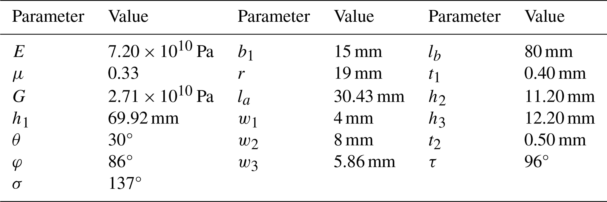
The relevant parameters are as follows.

$$\begin{array}{}\text{(55)}& \begin{array}{rl}& {\mathbf{M}}_{\mathrm{1}}=-{\mathbf{\Gamma }}_{\mathrm{5}}^{-\mathrm{1}}\cdot {\mathbf{\Gamma }}_{\mathrm{17}}\\ & {\mathbf{M}}_{\mathrm{13}}={\mathbf{\Gamma }}_{\mathrm{16}}+{\mathbf{M}}_{\mathrm{7}}\cdot {\mathbf{M}}_{\mathrm{10}}\\ & {\mathbf{M}}_{\mathrm{2}}=-{\mathbf{\Gamma }}_{\mathrm{5}}^{-\mathrm{1}}\cdot {\mathbf{\Gamma }}_{\mathrm{21}}\\ & {\mathbf{M}}_{\mathrm{14}}={\mathbf{M}}_{\mathrm{8}}+{\mathbf{M}}_{\mathrm{7}}\cdot {\mathbf{M}}_{\mathrm{11}}\\ & {\mathbf{M}}_{\mathrm{3}}=-{\mathbf{\Gamma }}_{\mathrm{7}}^{-\mathrm{1}}\cdot {\mathbf{\Gamma }}_{\mathrm{19}}{\mathbf{M}}_{\mathrm{15}}=-{\mathbf{M}}_{\mathrm{14}}^{-\mathrm{1}}\cdot {\mathbf{M}}_{\mathrm{12}}\\ & {\mathbf{M}}_{\mathrm{4}}=-{\mathbf{\Gamma }}_{\mathrm{7}}^{-\mathrm{1}}\cdot {\mathbf{\Gamma }}_{\mathrm{23}}{\mathbf{M}}_{\mathrm{16}}=-{\mathbf{M}}_{\mathrm{14}}^{-\mathrm{1}}\cdot {\mathbf{M}}_{\mathrm{13}}\\ & {\mathbf{M}}_{\mathrm{5}}=-{\mathbf{\Gamma }}_{\mathrm{2}}+{\mathbf{\Gamma }}_{\mathrm{14}}\cdot {\mathbf{M}}_{\mathrm{1}}+{\mathbf{\Gamma }}_{\mathrm{18}}\cdot {\mathbf{M}}_{\mathrm{3}}\\ & {\mathbf{M}}_{\mathrm{17}}={\mathbf{M}}_{\mathrm{9}}+{\mathbf{M}}_{\mathrm{11}}\cdot {\mathbf{M}}_{\mathrm{15}}\\ & {\mathbf{M}}_{\mathrm{6}}={\mathbf{\Gamma }}_{\mathrm{14}}\cdot {\mathbf{M}}_{\mathrm{2}}+{\mathbf{\Gamma }}_{\mathrm{18}}\cdot {\mathbf{M}}_{\mathrm{4}}\end{array}\end{array}$$

$$\begin{array}{rl}& {\mathbf{M}}_{\mathrm{18}}={\mathbf{M}}_{\mathrm{10}}+{\mathbf{M}}_{\mathrm{11}}\cdot {\mathbf{M}}_{\mathrm{16}}\\ & {\mathbf{M}}_{\mathrm{7}}={\mathbf{\Gamma }}_{\mathrm{20}}\cdot {\mathbf{M}}_{\mathrm{1}}+{\mathbf{\Gamma }}_{\mathrm{22}}\cdot {\mathbf{M}}_{\mathrm{3}}\\ & {\mathbf{M}}_{\mathrm{19}}={\mathbf{\Gamma }}_{\mathrm{1}}+{\mathbf{\Gamma }}_{\mathrm{8}}\cdot {\mathbf{M}}_{\mathrm{17}}+{\mathbf{\Gamma }}_{\mathrm{10}}\cdot {\mathbf{M}}_{\mathrm{15}}\\ & {\mathbf{M}}_{\mathrm{8}}={\mathbf{\Gamma }}_{\mathrm{4}}+{\mathbf{\Gamma }}_{\mathrm{20}}\cdot {\mathbf{M}}_{\mathrm{2}}+{\mathbf{\Gamma }}_{\mathrm{22}}\cdot {\mathbf{M}}_{\mathrm{4}}\\ & {\mathbf{M}}_{\mathrm{20}}={\mathbf{\Gamma }}_{\mathrm{8}}\cdot {\mathbf{M}}_{\mathrm{18}}+{\mathbf{\Gamma }}_{\mathrm{10}}\cdot {\mathbf{M}}_{\mathrm{16}}\\ & {\mathbf{M}}_{\mathrm{9}}=-{\mathbf{M}}_{\mathrm{5}}^{-\mathrm{1}}\cdot {\mathbf{\Gamma }}_{\mathrm{9}}{\mathbf{M}}_{\mathrm{21}}={\mathbf{\Gamma }}_{\mathrm{12}}\cdot {\mathbf{M}}_{\mathrm{17}}+{\mathbf{\Gamma }}_{\mathrm{15}}\cdot {\mathbf{M}}_{\mathrm{15}}\\ & {\mathbf{M}}_{\mathrm{10}}=-{\mathbf{M}}_{\mathrm{5}}^{-\mathrm{1}}\cdot {\mathbf{\Gamma }}_{\mathrm{11}}\\ & {\mathbf{M}}_{\mathrm{22}}={\mathbf{\Gamma }}_{\mathrm{3}}+{\mathbf{\Gamma }}_{\mathrm{12}}\cdot {\mathbf{M}}_{\mathrm{18}}+{\mathbf{\Gamma }}_{\mathrm{15}}\cdot {\mathbf{M}}_{\mathrm{16}}\\ & {\mathbf{M}}_{\mathrm{11}}=-{\mathbf{M}}_{\mathrm{5}}^{-\mathrm{1}}\cdot {\mathbf{M}}_{\mathrm{6}}{\mathbf{M}}_{\mathrm{23}}={\mathbf{M}}_{\mathrm{21}}-{\mathbf{M}}_{\mathrm{22}}\cdot {\mathbf{M}}_{\mathrm{20}}^{-\mathrm{1}}\cdot {\mathbf{M}}_{\mathrm{19}}\\ & {\mathbf{M}}_{\mathrm{12}}={\mathbf{\Gamma }}_{\mathrm{13}}+{\mathbf{M}}_{\mathrm{7}}\cdot {\mathbf{M}}_{\mathrm{9}}\end{array}$$

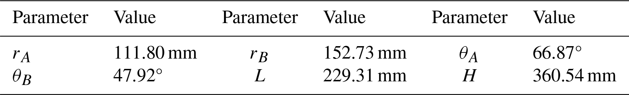
Table 2 Structural parameters of the 6-DOF compliant manipulator.

Table 3 The 42 error parameters randomly generated by MATLAB.

Figure 13 The results of the error identification: panels (a)–(f) are the six chains.

4.3 FEM simulations

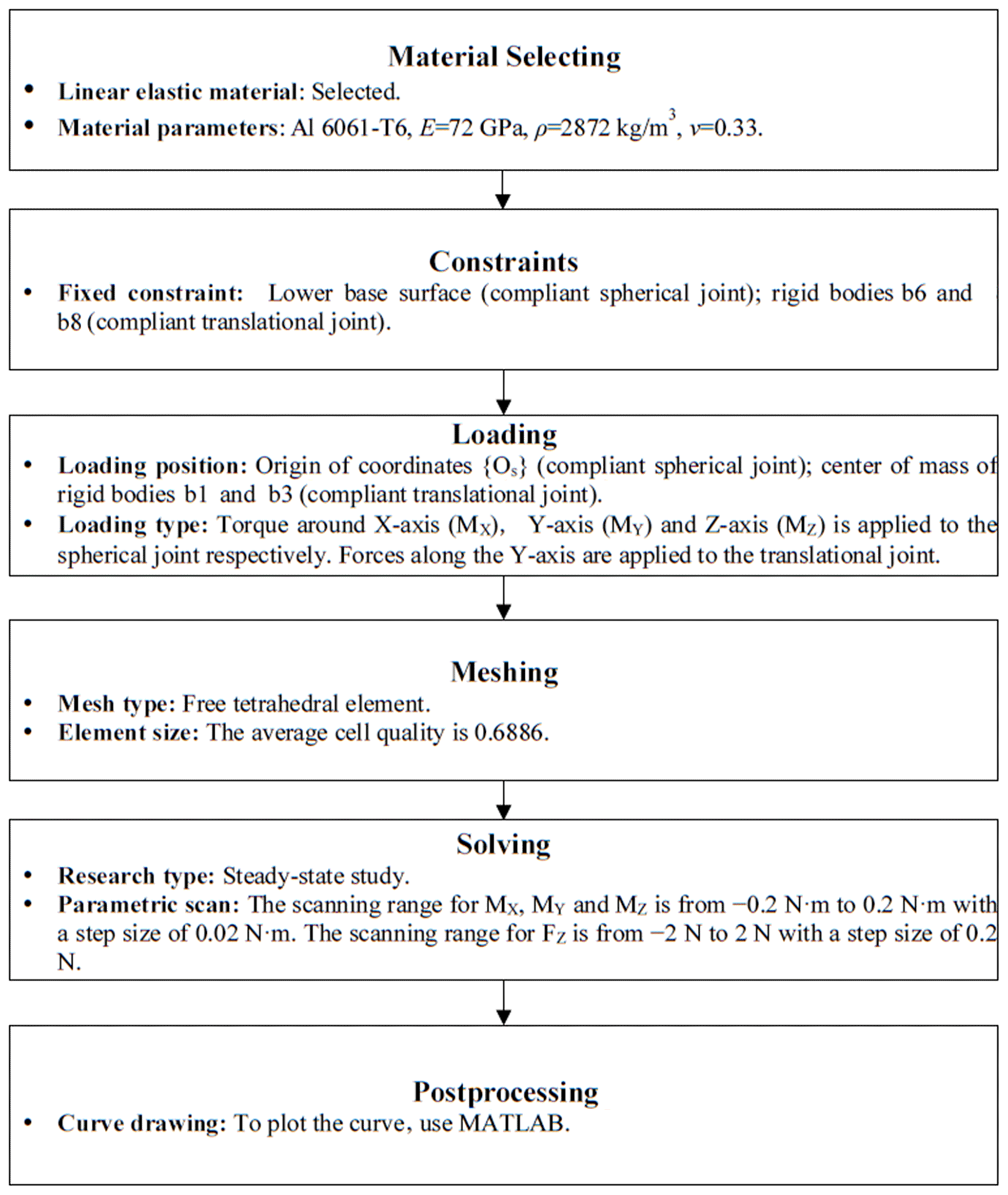
To validate the accuracy of the kinetostatic analysis model for the compliant joints, FEM simulations are conducted. The specific process is illustrated in Fig. 11, with the structural parameters detailed in Table 1.

To elucidate the relationship between the input load and the output displacement of the compliant spherical joint under various loading conditions, Fig. 12a depicts the relationship between the input load and output displacement of the compliant spherical joint in a moment around the x axis. Similarly, Fig. 12b and c display the results for moments around the y and z axes, respectively. From the figure, it can be concluded that the average error between the results of the static model and the FEM simulation is less than 5.6 %. Figure 12d shows the results under load along the y axis, with a high curve overlap and a maximum error of 4.4 %.

5 Manufacture error identification

Based on the analytical kinematic model derived in Sect. 4, this section presents an error identification model for the 6-DOF compliant parallel manipulator using the closed-loop vector method and conducts simulations. Iterative solutions are performed using the least-squares method and the Levenberg–Marquardt optimization algorithm based on randomly generated error parameters and pose data. Simulation results are compared with the random error parameters to verify the accuracy of the error identification model.

5.1 Residual equation

For kinematic modeling of the 6-DOF parallel manipulator, only the coordinates of the upper joint points (A_ix, A_iy, A_iz), lower joint points (B_ix, B_iy, B_iz) and leg lengths L_i are required for solving. Typically, the pose errors of the moving platform are primarily caused by these parameters, and kinematic calibration involves error identification and compensation for these 42 parameters. Let u_i= [A_ix, A_iy, A_iz, B_ix, B_iy, B_iz]^T.

Initially, a residual equation must be constructed. Given an input displacement d_p, let X_p be the actual pose of the moving platform and ${\mathbf{X}}_p^{{}^{\prime }}$ the theoretical pose obtained from the forward kinematic model, leading to the residual equation

$$\begin{array}{}\text{(56)}& {\mathit{f}}_p={\mathbf{X}}_p-{\mathbf{X}}_p^{{}^{\prime }}.\end{array}$$

While constructing the residual equation in this manner is straightforward and intuitive, it involves forward kinematic computations, leading to low computational efficiency. Hence, constructing the residual equation based on input displacement is preferred. Let Δl_ip be the actual input displacement for the ith actuator and $\mathrm{\Delta }{l}_{ip}^{{}^{\prime }}$ be the theoretical input displacement solved using the inverse kinematic model (Eq. 7). Where structural errors exist, theoretical and actual input displacements will deviate; the deviation disappears only when the theoretical and actual structural parameters are identical. Thus, the residual function for the ith input displacement at the pth pose is

$$\begin{array}{}\text{(57)}& f_{ip}=f_{ip}\left({\mathit{u}}_i\right)=\mathrm{\Delta }{l}_{ip}-\mathrm{\Delta }{l}_{ip}^{{}^{\prime }}.\end{array}$$

The residual functions for the six chains are combined as

$$\begin{array}{}\text{(58)}& F\left(\mathit{u}\mathbf{\right)}=[f_{\mathrm{11}}{f}_{\mathrm{21}}\mathrm{\cdots }{f}_{i,p}\mathrm{\cdots }{f}_{\mathrm{6}m}{]}_{\mathrm{6}m\times \mathrm{1}}^{\mathrm{T}},\end{array}$$

where u = [u₁ u₂... u₆]^T, with m being the total number of poses.

Based on the least-square principle, the residual function f_ip from Eq. (59) forms the evaluation function

$$\begin{array}{}\text{(59)}& e=\sum _{p=\mathrm{1}}^m\sum _{i=\mathrm{1}}^{\mathrm{6}}{f}_{ip}^{\mathrm{2}}.\end{array}$$

A smaller value of the evaluation function e indicates a reduced disparity between the input displacement calculated using the inverse kinematic model and the actual input displacement, suggesting that the solved structural parameter u is closer to their actual values.

5.2 Jacobian matrix

Optimization of the residual equation necessitates the construction of the Jacobian matrix, which is composed of first-order partial derivatives arranged in a specific configuration. This matrix represents the best linear approximation of a differentiable equation at a given point, often indicating the search direction for optimization algorithms. Equation (6) is rewritten as

$$\begin{array}{}\text{(60)}& \begin{array}{rl}& L_i^{\mathrm{2}}={\left({}^{\mathrm{B}}{\mathbf{R}}_{\mathrm{A}}{\mathit{A}}_i+{}^{\mathrm{B}}{\mathbf{P}}_{\mathrm{A}}-\left({\mathbf{B}}_i+\mathrm{\Delta }{l}_i{\mathit{q}}_i\right)\right)}^{\mathrm{T}}\\ & \left({}^{\mathrm{B}}{\mathbf{R}}_{\mathrm{A}}{\mathit{A}}_i+{}^{\mathrm{B}}{\mathbf{P}}_{\mathrm{A}}-\left({\mathbf{B}}_i+\mathrm{\Delta }{l}_i{\mathit{q}}_i\right)\right).\end{array}\end{array}$$

Differentiating both sides of Eq. (35) yields

$$\begin{array}{}\text{(61)}& \begin{array}{rl}& \mathrm{2}{L}_i\mathrm{d}{L}_i=\mathrm{2}{\left({}^{\mathrm{B}}{\mathbf{R}}_{\mathrm{A}}{\mathit{A}}_i+{}^{\mathrm{B}}{\mathbf{P}}_{\mathrm{A}}-{\mathbf{B}}_i-\mathrm{\Delta }{l}_i{\mathit{q}}_i\right)}^{\mathrm{T}}\\ & \left({}^{\mathrm{B}}{\mathbf{R}}_{\mathrm{A}}\mathrm{d}{\mathit{A}}_i-\mathrm{d}{\mathbf{B}}_i-\mathrm{d}\mathrm{\Delta }{l}_i{\mathit{q}}_i-\mathrm{\Delta }{l}_i\mathrm{d}{\mathit{q}}_i\right)\\ & =\mathrm{2}{\mathit{v}}_i\left({}^{\mathrm{B}}{\mathbf{R}}_{\mathrm{A}}\mathrm{d}{\mathit{A}}_i-\mathrm{d}{\mathbf{B}}_i-\mathrm{d}\mathrm{\Delta }{l}_i{\mathit{q}}_i-\mathrm{\Delta }{l}_i\mathrm{d}{\mathit{q}}_i\right),\end{array}\end{array}$$

where d represents a small change in a variable. Assuming that the driving direction of the actuator is sufficiently precise, let dq_i=0. From Eq. (61), we obtain

$$\begin{array}{}\text{(62)}& \mathrm{d}\mathrm{\Delta }{l}_i={\displaystyle \frac{{\mathit{v}}_i^{\mathrm{B}}{\mathbf{R}}_{\mathrm{A}}}{{\mathit{v}}_i{\mathit{q}}_i}}\mathrm{d}{\mathit{A}}_i-{\displaystyle \frac{{\mathit{v}}_i}{{\mathit{v}}_i{\mathit{q}}_i}}\mathrm{d}{\mathit{B}}_i-{\displaystyle \frac{L_i}{{\mathit{v}}_i{\mathit{q}}_i}}\mathrm{d}{L}_i.\end{array}$$

Organized in matrix form, this is

$$\begin{array}{}\text{(63)}& \mathrm{d}\mathrm{\Delta }{l}_i=\left[\begin{array}{ccc}\frac{{\mathit{v}}_i^{\mathrm{B}}{\mathbf{R}}_{\mathrm{A}}}{{\mathit{v}}_i{\mathit{q}}_i}& \frac{{\mathit{v}}_i}{{\mathit{v}}_i{\mathit{q}}_i}& \frac{L_i}{{\mathit{v}}_i{\mathit{q}}_i}\end{array}\right]\left[\begin{array}{l}\mathrm{d}{\mathit{A}}_i\\ \mathrm{d}{\mathit{B}}_i\\ \mathrm{d}{L}_i\end{array}\right].\end{array}$$

Combining the six closed-loop kinematic chains results in

$$\begin{array}{}\text{(64)}& \mathrm{d}\mathrm{\Delta }\mathit{l}=\mathbf{J}\mathrm{d}\mathit{u},\end{array}$$

where $\mathrm{d}\mathrm{\Delta }\mathit{l}=[\mathrm{d}\mathrm{\Delta }{l}_{\mathrm{1}}\mathrm{d}\mathrm{\Delta }{l}_{\mathrm{2}}\mathrm{d}\mathrm{\Delta }{l}_{\mathrm{3}}\mathrm{d}\mathrm{\Delta }{l}_{\mathrm{4}}\mathrm{d}\mathrm{\Delta }{l}_{\mathrm{5}}\mathrm{d}\mathrm{\Delta }{l}_{\mathrm{6}}{]}^{\mathrm{T}}\in {\mathbf{R}}^{\mathrm{6}\times \mathrm{1}}$ is the input displacement residual calculated from Eq. (57), $\mathrm{d}\mathit{u}\mathbf{=}[\mathrm{d}{\mathit{A}}_{\mathrm{1}}\mathrm{d}{\mathbf{B}}_{\mathrm{1}}\mathrm{d}{L}_{\mathrm{1}}\mathrm{\cdots }\mathrm{d}{\mathit{A}}_{\mathrm{6}}\mathrm{d}{\mathbf{B}}_{\mathrm{6}}\mathrm{d}{L}_{\mathrm{6}}{]}^{\mathrm{T}}\in {\mathbf{R}}^{\mathrm{42}\times \mathrm{1}}$ includes joint point errors and leg length errors, and J is the Jacobian matrix. Specifically,

$$\begin{array}{}\text{(65)}& \mathbf{J}=\left[\begin{array}{ccccc}\frac{{\mathit{v}}_{\mathrm{1}}^{\mathrm{B}}{\mathbf{R}}_{\mathrm{A}}}{{\mathit{v}}_{\mathrm{1}}{\mathit{q}}_{\mathrm{1}}}& \frac{{\mathit{v}}_{\mathrm{1}}}{{\mathit{v}}_{\mathrm{1}}{\mathit{q}}_{\mathrm{1}}}& \frac{L_{\mathrm{1}}}{{\mathit{v}}_{\mathrm{1}}{\mathit{q}}_{\mathrm{1}}}& \mathrm{0}& \mathrm{0}\\ \mathrm{0}& \mathrm{\cdots }& \mathrm{0}& \mathrm{0}& \mathrm{0}\\ \mathrm{0}& \mathrm{0}& \mathrm{0}& \frac{{\mathit{v}}_{\mathrm{2}}^{\mathrm{B}}{\mathbf{R}}_{\mathrm{A}}}{{\mathit{v}}_{\mathrm{2}}{\mathit{q}}_{\mathrm{2}}}& \frac{{\mathit{v}}_{\mathrm{2}}}{{\mathit{v}}_{\mathrm{2}}{\mathit{q}}_{\mathrm{2}}}\\ \frac{L_{\mathrm{2}}}{{\mathit{v}}_{\mathrm{2}}{\mathit{q}}_{\mathrm{2}}}& \mathrm{\cdots }& \mathrm{0}& \mathrm{0}& \mathrm{0}\\ \mathrm{⋮}& \mathrm{⋮}& \mathrm{⋮}& \mathrm{⋮}& \mathrm{⋮}\\ \mathrm{⋮}& \mathrm{\ddots }& \mathrm{⋮}& \mathrm{⋮}& \mathrm{⋮}\\ \mathrm{0}& \mathrm{0}& \mathrm{0}& \mathrm{0}& \mathrm{0}\\ \mathrm{0}& \mathrm{\cdots }& \frac{{\mathit{v}}_{\mathrm{6}}^{\mathrm{B}}{\mathbf{R}}_{\mathrm{A}}}{{\mathit{v}}_{\mathrm{6}}{\mathit{q}}_{\mathrm{6}}}& \frac{{\mathit{v}}_{\mathrm{6}}}{{\mathit{v}}_{\mathrm{6}}{\mathit{q}}_{\mathrm{6}}}& \frac{L_{\mathrm{6}}}{{\mathit{v}}_{\mathrm{6}}{\mathit{q}}_{\mathrm{6}}}\end{array}\right].\end{array}$$

Solving the error identification model is a complex nonlinear least-square problem. The Gauss–Newton method, derived from the classical Newton method, is often employed to solve such problems. It replaces the computationally intensive and difficult-to-calculate Hessian matrix in the Newton method with the first-order derivative term J^TJ. It enhances the computational efficiency and is widely used in data fitting, parameter estimation and machine learning. Its iterative formula is

$$\begin{array}{}\text{(66)}& {\mathit{u}}^{(\mathrm{k}+\mathrm{1})}={\mathit{u}}^{\left(\mathrm{k}\right)}-({\mathbf{J}}^{\mathrm{T}}\mathbf{J}{)}^{-\mathrm{1}}\cdot {\mathbf{J}}^{\mathrm{T}}\mathrm{d}\mathrm{\Delta }\mathit{l},\end{array}$$

where, if J^TJ is non-invertible or ill-conditioned, the search direction's magnitude becomes very large, preventing the algorithm's progression. To overcome this issue, the Levenberg–Marquardt method, which introduces a damping coefficient matrix a I into the ill-conditioned matrix, is used to avoid excessively large search direction magnitudes. The specific formula is

$$\begin{array}{}\text{(67)}& {\mathit{u}}^{(k+\mathrm{1})}={\mathit{u}}^{\left(k\right)}-({\mathbf{J}}^{\mathrm{T}}\mathbf{J}+a_{\mathrm{k}}\mathbf{I}{)}^{-\mathrm{1}}\cdot {\mathbf{J}}^{\mathrm{T}}\mathrm{d}x,\end{array}$$

where a_k is the damping coefficient and I is the identity matrix.

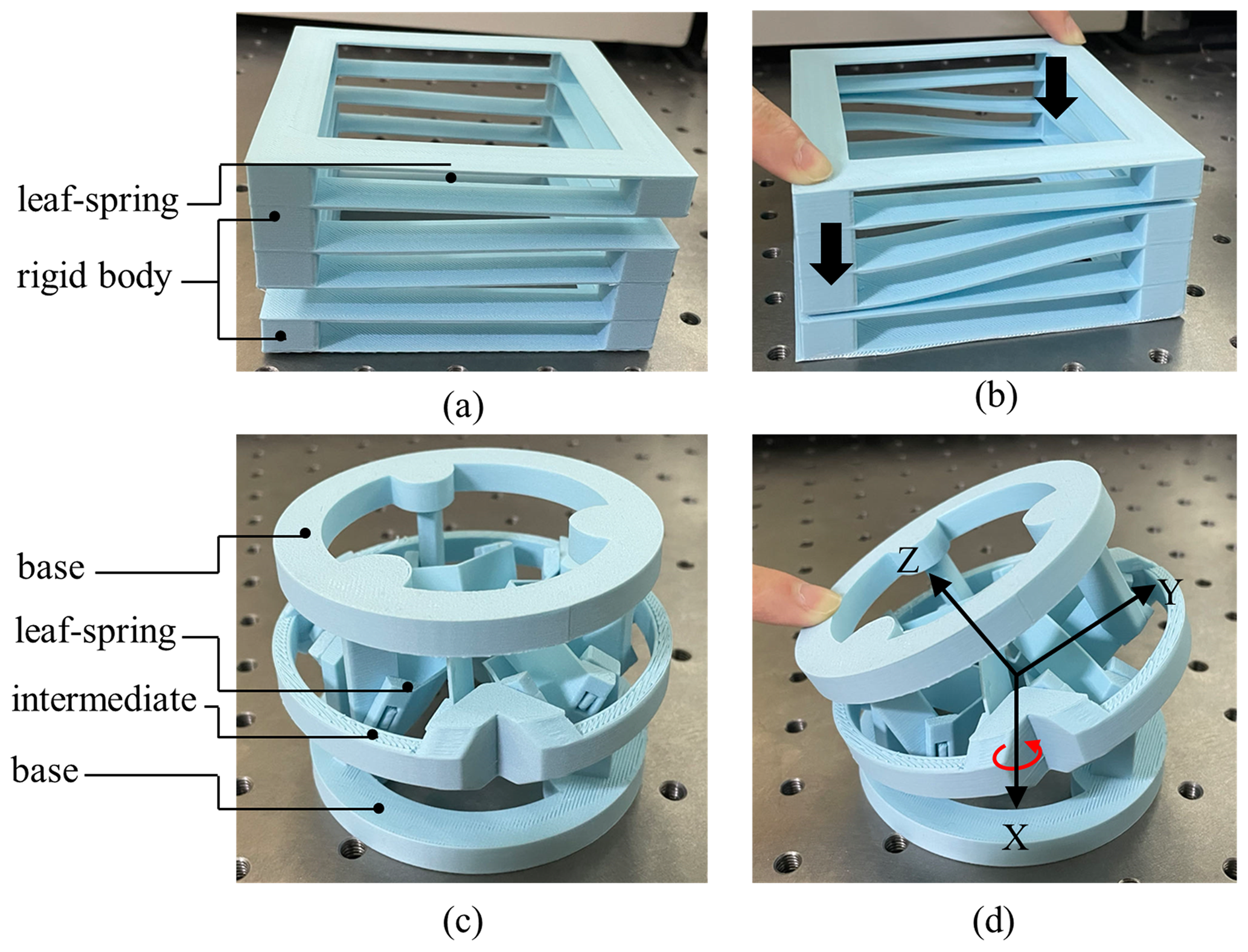
Figure 14 Three-dimensional printing of compliant joints: (a) the compliant translational joint, (b) translational motion of the compliant translational joint, (c) the compliant spherical joint and (d) tilt motion of the compliant spherical joint.

5.3 Simulation verification

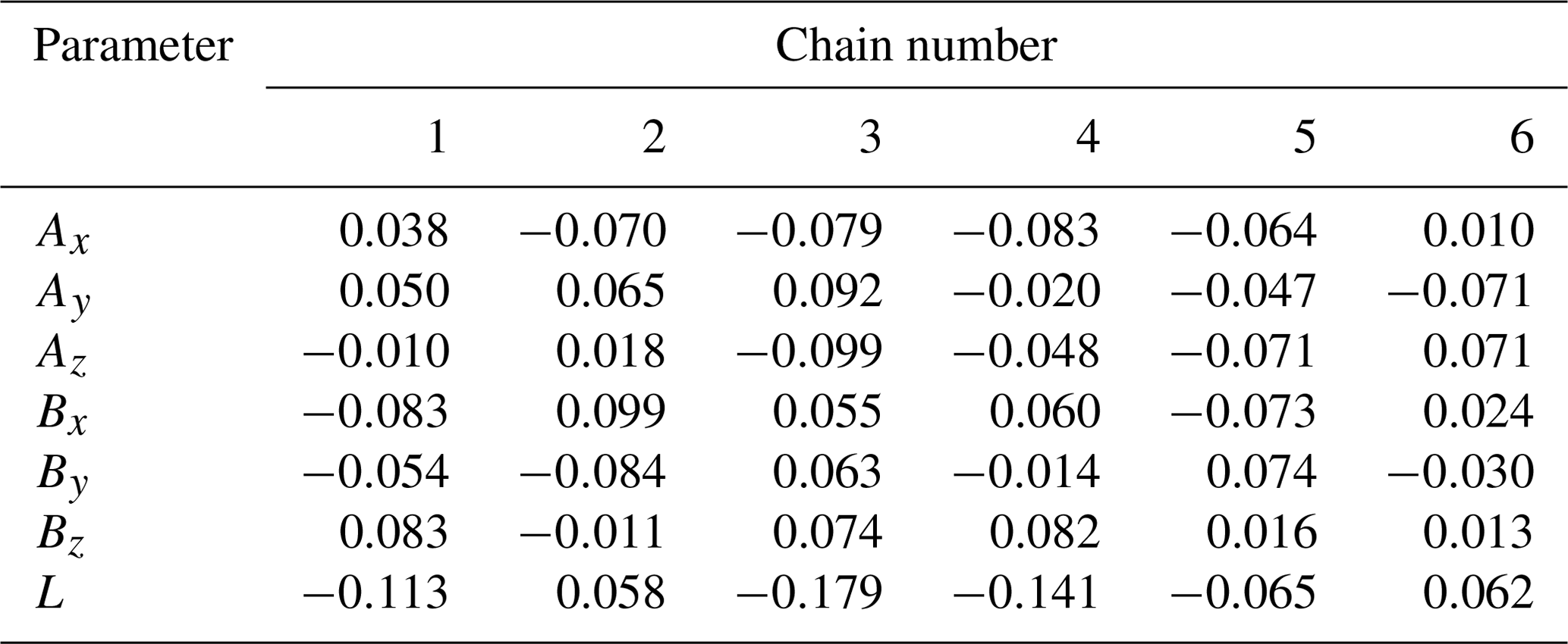
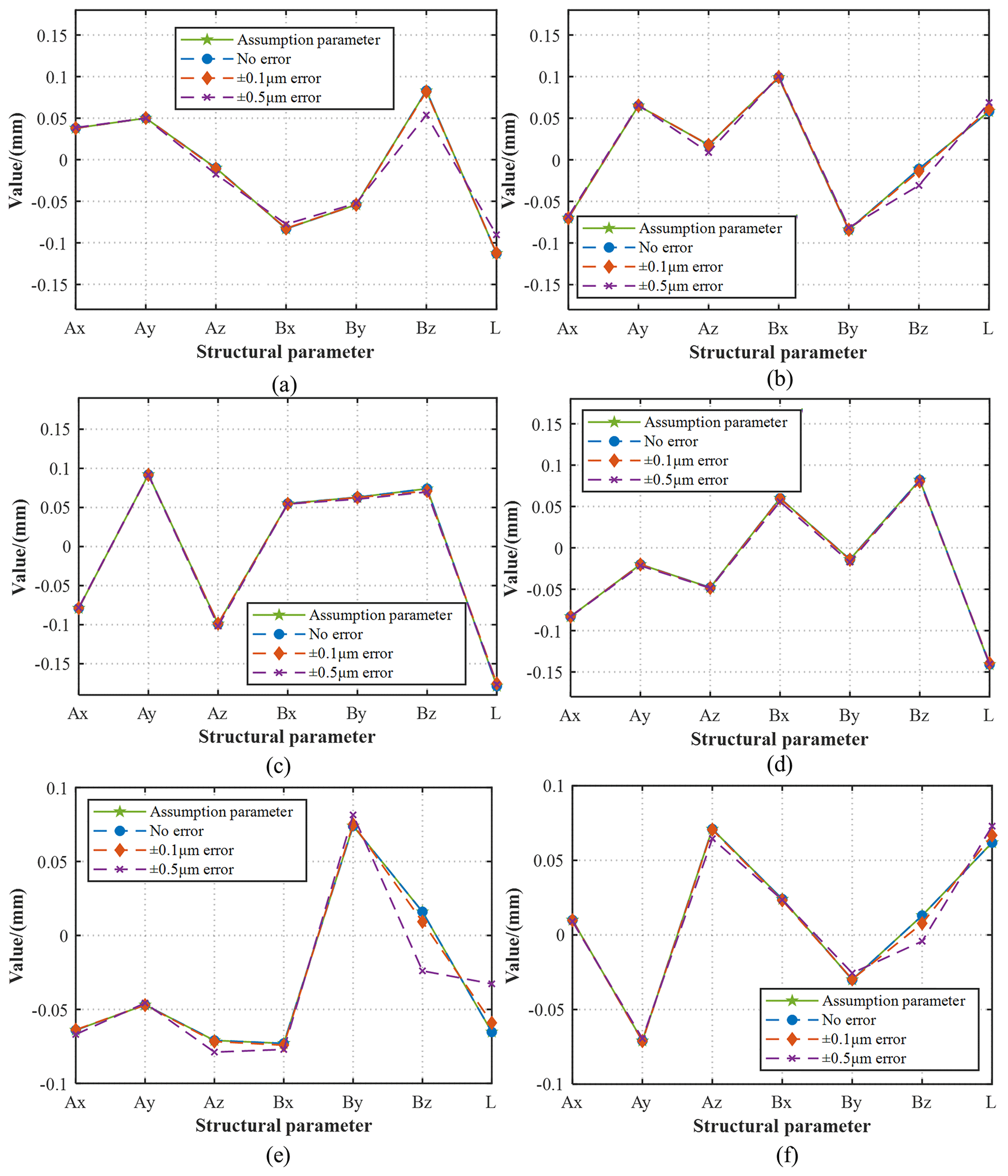
For error identification simulation, errors are added to the ideal structural parameters u to simulate actual conditions. The ideal structural parameters are shown in Table 2. Using MATLAB2023a, 36 random deviation parameters ranging from −0.1 to 0.1 mm are generated and integrated as deviations into the joint point coordinates. Solving for the joint point coordinates with these added errors results in six leg length errors. These 42 error parameters (Table 3) serve as a target for error identification. Additionally, 40 sets of poses are randomly generated as the input sample set for the error identification model, with position variations from −20 to 20 mm and angular variations from −15 to 15°. The simulation is conducted according to the steps mentioned above, without considering the measurement noise. However, considering the precision of the existing measurement instruments, errors may occur during pose measurement. Therefore, in the simulation process, random measurement noise is introduced into the 40 sets of configurations, ranging from −0.1 to 0.1 µm and from −0.5 to 0.5 µm, respectively. The simulation results are shown in Fig. 13. The results indicate that, when there is no measurement error in the pose samples, the error identification model can accurately solve all structural error parameters, with a maximum identification accuracy of up to 10⁻¹² mm. Even with added measurement noise within the range from −0.1 to 0.1 µm, the error model still reliably identifies the structural error parameters, with a maximum identification accuracy of up to 10⁻⁵ mm. However, with the introduced measurement noise spanning from −0.5 to 0.5 µm, notable discrepancies arise in the identification of certain structural deviation parameters. This indicates that the precision of the pose measurement impacts the error identification model, necessitating control of measurement errors within a certain range.

6 Conclusions

This paper introduces a new 6-DOF compliant parallel manipulator featuring a 6-PSS configuration. This design strategically mounts six actuators directly on the base, reducing the moving mass, enhancing the response speed, and contributing to superior dynamic performance. To further enhance the motion accuracy, the manipulator employs compliant joints instead of traditional rigid-body joints to mitigate issues related to friction and backlash. Notably, this manipulator incorporates leaf spring compliant joints with distributed compliance, broadening the motion range relative to compliant joints with lumped compliance. Kinetostatic modeling of these compliant joints employs the matrix displacement method, aligning closely with FEM analysis results, which show an average discrepancy of 5.5 %. Comprehensive kinematic modeling of the entire manipulator has been conducted, providing both forward and inverse kinematic solutions. Subsequent analyses delve into manufacture error identification, encompassing the development and resolution of a manufacture error identification model validated through FEM simulations and accounting for measurement noise and errors. Future work will optimize the geometric dimensions of the 6-DOF compliant parallel manipulator based on its kinematic and dynamic models, followed by manufacturing and experimental testing of the manipulator system. The advanced features of the proposed 6-DOF compliant parallel manipulator, such as its high precision and relatively large motion range, render it ideally suited for critical applications in precision engineering fields like chip manufacturing and packaging.

At present, this work has completed 3D printing of compliant joints, as shown in Fig. 14.