A convolutional neural-network-based diagnostic framework for industrial bearing

The problem of industrial bearing health monitoring and fault diagnosis has recently been a popular research topic. Extracting sufficient features from the input raw vibration signals and mapping them to the most likely fault labels is the essence of bearing fault diagnosis. This study proposes a novel framework for bearing defect diagnostics by merging dilated residual convolutional neural networks and attention mechanisms. In this framework, multiple parallel dilated convolutional networks can automatically learn rich fault features at each scale from vibration signals. Simultaneously, the attention approach boosts fault-related features and suppresses irrelevant ones, improving fault detection performance and generalization. According to the experimental results of two different bearing datasets, the framework achieves a higher accuracy and can accurately identify various types of faults.

1 Introduction

With the advent of the era of big industrial data, mechanical equipment is constantly developing toward complexity and intelligence. As a basic component of mechanical equipment, industrial bearings are also components with a high incidence of failure. Industrial bearing failure can directly lead to the deterioration of the operating condition of mechanical equipment and pose significant safety issues. Based on statistics, bearing failures account for 40 %–70 % of the electro-mechanical drive system, resulting in substantial losses (Lessmeier et al., 2016). Therefore, real-time and accurate diagnostics of industrial bearings are critical for ensuring smooth operation and extending the equipment's life.

The commonly used methods for industrial bearing diagnosis include oil pressure, infrared thermal imaging, vibroacoustic measurements, electric current, etc. (Thoppil et al., 2021). Since low-cost vibration sensors can conveniently collect a wide range of vibration fault information, vibration-signal-based diagnostic methods are most widely adopted in health condition monitoring. The fault signals of industrial bearings are non-smooth and contain a lot of background noise (Lin et al., 2004), and the defects are rarely single. It is a great challenge for the diagnosis model to extract the effective fault information from the complex vibration signal and ensure classification accuracy. Bearing fault diagnosis models usually have two major parts: feature extraction and fault classification (Chen et al., 2021). Feature extraction refers to the extraction of representative fault-related information from the raw data based on the technicians' signal processing knowledge and practical engineering experience, usually divided into time and frequency domain information.

A single time-domain signal often cannot accurately express bearing fault information. It is common to transform it into the frequency domain or time–frequency domain, such as wavelet packet (Yen and Lin, 2000), envelope analysis (Tsao et al., 2012), and empirical mode decomposition distribution (Yu and Junsheng, 2006). Various machine learning algorithms are used as classifiers on the extracted fault features, such as support vector machines (SVMs) (Yang et al., 2007), random forest methods (Roy et al., 2020), and K nearest neighbor (KNN) (Tian et al., 2015).

Fault diagnosis models based on shallow machine learning techniques and manual feature extraction methods have shown excellent recognition accuracy. However, there are several clear drawbacks: (1) it needs to manually extract features from the original vibration signal based on experience and signal processing knowledge, which requires intensive computation. What's more, the effect of diagnosis mainly depends on the quality of feature extraction. (2) Feature extraction and classification are two independent processes, and the unsynchronized extraction and classification cannot meet the requirements of real-time diagnosis in the production system. (3) The diagnostic capability of shallow machine learning is slightly insufficient in the face of massive and strongly dynamic data, making it difficult to adapt to complex working conditions (Jiao et al., 2020).

The rapid development of deep learning has brought a new approach to bearing fault diagnosis. As a common deep learning model, the convolutional neural network (CNN) has achieved remarkable results in object recognition, image processing, and audio classification (Khan et al., 2020). Due to its multi-layer network structure, CNN has a strong adaptive feature learning ability, does not require any complicated manual extraction process, and can automatically learn fault feature representations from raw signal data.

Zhu et al. (2019) transformed the original one-dimensional time-domain signal into a time–frequency map through a short-time Fourier transform and input it into a convolutional neural network to identify fault features. Wang et al. (2019) compared the classification performance of eight different time–frequency analysis methods on the AlexNet model.

Mechanical equipment conditions are complicated and varied throughout the operation, and bearing failures come in various shapes and locations. As a result, the signal contains multiple scales of characteristics. Jiang et al. (2018) introduced multi-scale coarse-grained layers in CNNs to capture different granularity features by smooth shifting. Peng et al. (2020) offered a multi-branch, multi-scale CNN for learning rich and complementary defect information from wheel set bearings. Multi-scale convolutional networks have more layers and are susceptible to degradation. Liu et al. (2019) incorporated residual learning into CNNs to improve model training and prevent performance deterioration. Surendran et al. (2022) utilized a residual multi-scale CNN model (inception-resnet v2) to extract high-level fault characteristics and optimize the parameters using the sailfish algorithm.

Motivated by the prior studies, we have developed a novel fault diagnostic framework, which incorporates multi-filter dilated CNNs, a residual convolutional neural network and attentional mechanisms. The framework enables automatic feature extraction and end-to-end detection for fault identification, enhancing CNN stability and generalization in complicated conditions. The following is a list of the paper's major contributions:

1. A multi-scale extraction module based on dilated CNNs is proposed. Dilated CNNs produce diverse receptive fields to capture different fault features by adjusting dilation rates.

2. We design the residual connection module to transfer feature information between different layers, enabling data from shallow levels to flow into deeper layers and reducing information loss during transmission. Additionally, a wide convolutional kernel is used to capture long-term dependencies and mitigate noise interference.

3. Multiple attention mechanisms are applied in the module. The attention module assigns different weights to captured fault features, thus enhancing representative features while suppressing irrelevant ones.

4. The diagnostic framework is proposed. It was validated under various scenarios with bearing vibration signals, and the effect of various dilation rates and reduction ratios on the model extraction capability was examined. It is experimentally demonstrated that the framework performs well in complex situations.

The following is the structure of this paper: Sect. 2 introduces the background knowledge of convolutional neural networks, Sect. 3 explains the diagnostic framework's components and its procedure, and Sect. 4 introduces the experimental datasets of Case Western Reserve University (CWRU) and Jiangnan University (JNU). Section 5 in this paper presents the experimental results under different tasks and their corresponding analyses. Conclusions are presented in Sect. 6.

2 Convolutional neural networks

Convolutional neural networks encompass three key concepts: sparse interaction, parameter sharing, and equi-variant representation (Goodfellow et al., 2016). As illustrated in Fig. 1, a typical convolutional neural network comprises convolutional, pooling, and fully connected layers.

Figure 1 Convolutional neural network architecture.

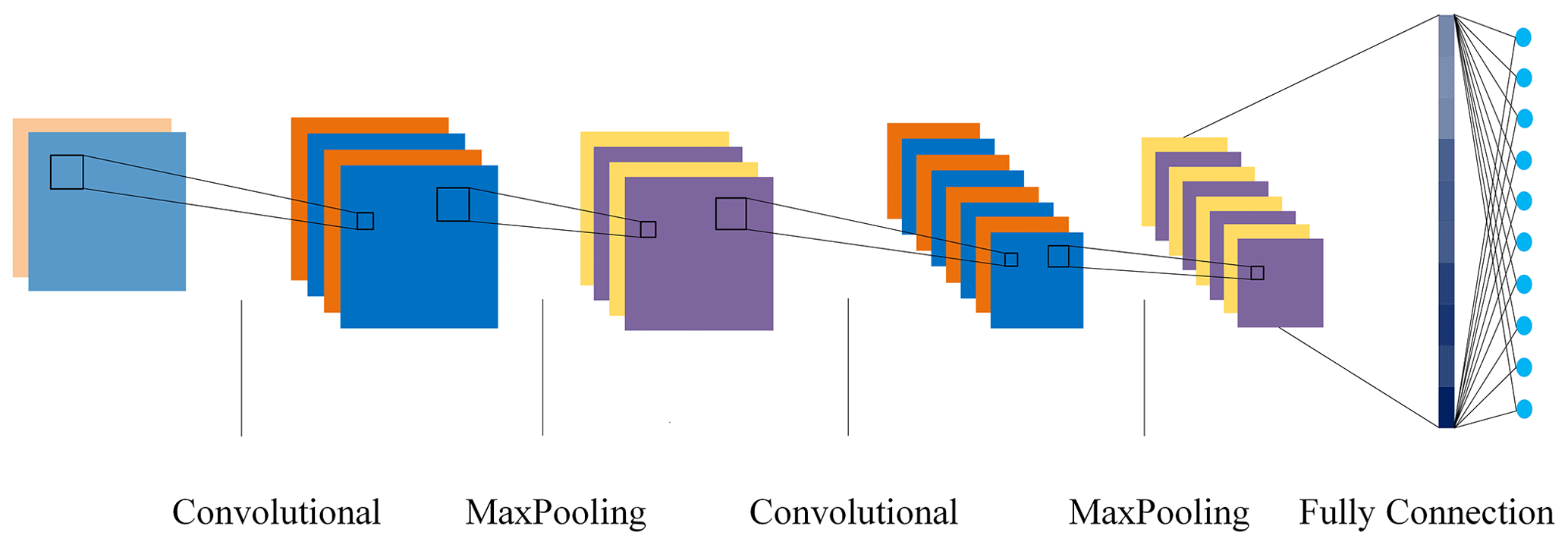
2.1 Feature extraction

The convolutional layer in CNNs stands as a cornerstone of its architecture. In this layer, input data are meticulously scanned using convolutional kernels. These kernels, akin to filters, possess a strong ability to discern intricate patterns within the data. Through the convolutional operation, these filters capture hierarchical and abstract representations of the input. Activation functions in CNNs map the inputs of neurons to their respective outputs. This transformation commonly employs nonlinear operations, enabling the network to learn the complex nonlinear relationships within the data. Pooling layers play a crucial role in simplifying computations within neural networks, which condense input dimensions by synthesizing local regions of the feature map into a single outcome. A CNN systematically extracts discriminative features related to faults from vibration signals by executing convolution and pooling operations.

2.2 Classification

After the feature extraction phase, the acquired features, refined through layers of convolutions and pooling, flow into densely connected layers, where intricate connections form, capturing abstract concepts. Each neuron in these fully connected layers acts as a learned feature detector, discerning complex combinations of visual elements. The final layer, often adorned with the softmax activation function, transforms these intricate features into probabilities, quantifying the network's confidence in each potential class.

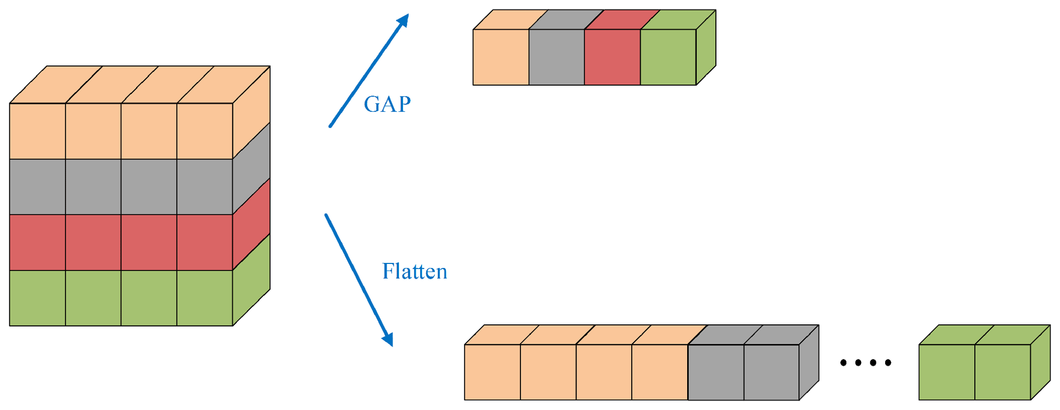
Traditional models often incorporate multiple fully connected layers to capture intricate dependencies within the data. However, as convolutional neural networks progress to depth and complexity, fully connected layers lead to a surge in parameters, which amplifies the risk of overfitting and puts forward higher requirements for the performance of diagnostic equipment. In response to the problem, Hinton et al. (2012) proposed the dropout method to randomly abandon the connection, reduce the co-adaptation between nodes, and empower the network to acquire robust features that generalize better to unseen data. To further improve the anti-fitting ability of the model and reduce the parameters in the training process, Lin et al. (2013) proposed a global average pooling method, which is different from the traditional fully connected layer by performing global average pooling on each feature map. Figure 2 compares the operational mechanisms of global average pooling and fully connected layers.

Figure 2 Comparison of fully connected layer and global average pooling.

3 Methods

3.1 Multi-filter dilated convolutional neural network

The vibration signal gathered by the accelerometer is typically non-stationary, meaning that the signal's frequency component fluctuates with time and has a significant degree of uncertainty. It comprises complex feature information of various timescales and presents typical multi-scale characteristics. Meanwhile, bearing faults come in various shapes and sizes, and different types of faults produce distinct characteristic frequencies. Due to these factors, traditional convolutional neural networks with a fixed filter do not extract enough information for accurate fault diagnosis.

We propose a multi-filter dilated convolution module to mine multi-scale information from the bearing vibration signals to perform the feature extraction work. The module's structure is depicted in Fig. 3. The module uses four parallel dilated convolution structures with a filter w, sliding in the vibration signal for convolutions to obtain multiple feature maps (Wang and Ji, 2018). It can get several receptive fields in the vibration signal sequence, allowing each output of the local convolution stage to catch different scale features, the formula being defined as

$$\begin{array}{}\text{(1)}& o=\sum _{s=\mathrm{1}}^{S}f[i+d\cdot s]w\left[i\right],\end{array}$$

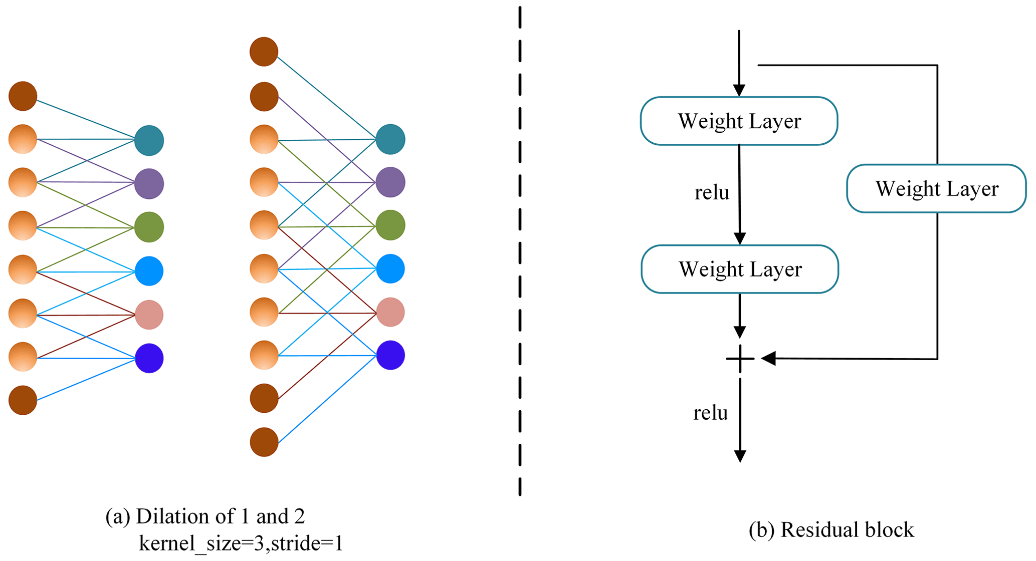
where d is the dilation rate and s denotes kernel size; the operation process of dilated convolution is depicted in Fig. 4a.

Figure 3 Multi-filter dilated convolutional neural network.

Figure 4 Dilated convolutional neural network and residual block.

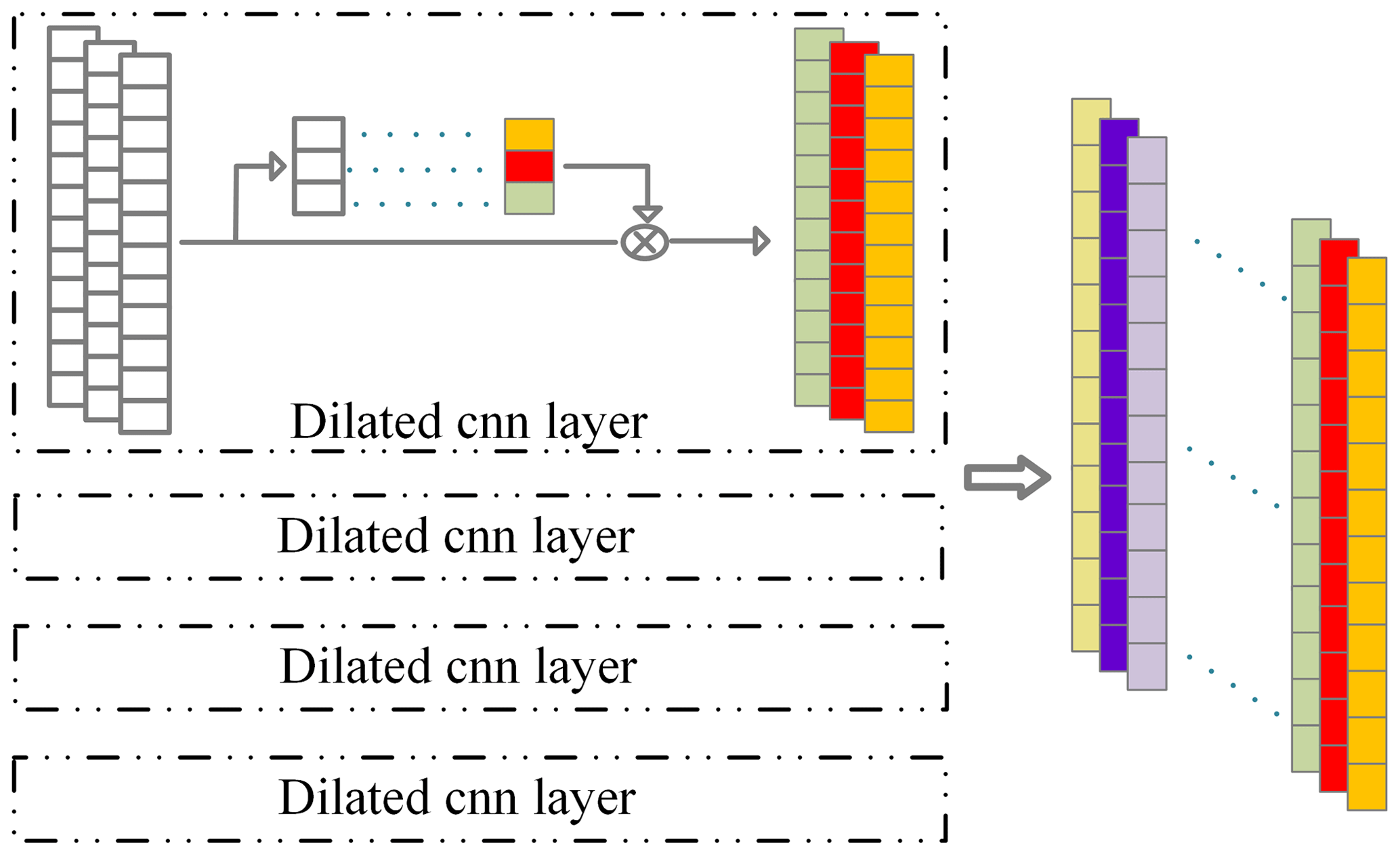
Given the diverse output sizes stemming from different dilation rates, we employ padding techniques to ensure uniform output lengths. Subsequently, feature maps from distinct levels are connected along the channel dimensions (Chen and Shi, 2021). Each structure is equipped with 64 filters and a kernel size of 5, so we can get the output in Eq. (2).

$$\begin{array}{}\text{(2)}& o=\left[o_{\mathrm{1}},o_{\mathrm{2}},\mathrm{\cdots },o_{n-h+\mathrm{1}}\right]\in R^{L\times C}\end{array}$$

Because the feature maps formed by convolution are substantially different in recognizing bearing fault features, we employ attention mechanism approaches to learn discriminative features and disregard valueless data. First, the global temporal information in the feature map of L length is compressed into a channel descriptor using the global average pooling layer (Hu et al., 2018).

$$\begin{array}{}\text{(3)}& z_c={\displaystyle \frac{\mathrm{1}}{L}}\sum _{i=\mathrm{1}}^L{o}_c\left(i\right),\end{array}$$

where z_c is channel-wise statistics, reflecting the global information of the c feature map.

To properly capture the correlation of the channels in the channel-wise statistics, the next step is to fuse the feature map information of each channel across the fully connection layer (Ye and Yu, 2021).

$$\begin{array}{}\text{(4)}& s=\mathit{\sigma }\left(F_{\mathrm{2}}\mathit{\delta }\left(F_{\mathrm{1}}z\right)\right),\end{array}$$

where δ represents the ReLU activation function, F₁ and F₂ denote the fully connected layers, and σ is the sigmoid that compresses the dynamic range of the vector between [0,1]. After that, channel-wise multiplication in Eq. (5) is performed to complete the rescaling of the original features in the channel dimension with the learned weights.

$$\begin{array}{}\text{(5)}& v\cdot s=\left[v_{\mathrm{1}}{s}_{\mathrm{1}},v_{\mathrm{2}}{s}_{\mathrm{2}},\mathrm{\cdots },v_c{s}_c\right]\end{array}$$

After extracting characteristics from each structure, they are combined across channels using concatenation.

3.2 Residual convolutional neural network

The residual network provides the shortcut connection approach (He et al., 2016) connecting earlier layers to later layers via shortcuts to allow the flow of information across distinct layers. Shortcut connections encompass identity and projection shortcuts, as illustrated in Eqs. (6)–(7).

$$\begin{array}{}\text{(6)}& {\displaystyle }y=F(x,W_i)+x,\text{(7)}& {\displaystyle }y=F(x,W_i)+W_{s}x,\end{array}$$

where y and x refer to input and output, F is residual mapping, and W_i indicates weight. The schematic diagram can be found in Fig. 4b.

We create a residual convolutional neural network that learns to integrate feature information from the 1D signal, which comprises convolutional layers with residual connections and a pooling layer. In designing our convolutional layers, we utilize a wider convolutional kernel of 32 for the initial filters to mitigate noise interference and capture global trend information more effectively (Liang and Zhao, 2021). Subsequently, the second layer employs filters with a kernel size of 7. The chosen number of filters for these convolutional layers are 128 and 256 to optimize the feature extraction capabilities of our model.

Due to the alteration in the number of channels across different layers, it is necessary to perform dimensional matching. This is accomplished via projection shortcuts as defined in Eq. (7), which employ a convolutional layer with a 1 × 1 kernel size to facilitate this transition. Finally, applying the ReLU activation function introduces nonlinearity into the model, enhancing its capacity to model complex functions.

3.3 Discriminative enhanced module

After the features are extracted by the multi-filter dilated and residual convolutional neural network, they are fused by element-wise addition. A discriminative enhanced module (DEM) is then applied to the extracted multi-level features to further deepen the model's ability to screen for critical features before entering the classification layer. The DEM module is shown in Fig. 5. It includes two branches: the spatial channel attention module and the channel attention module (Woo et al., 2018).

Figure 5 Discriminative enhanced module.

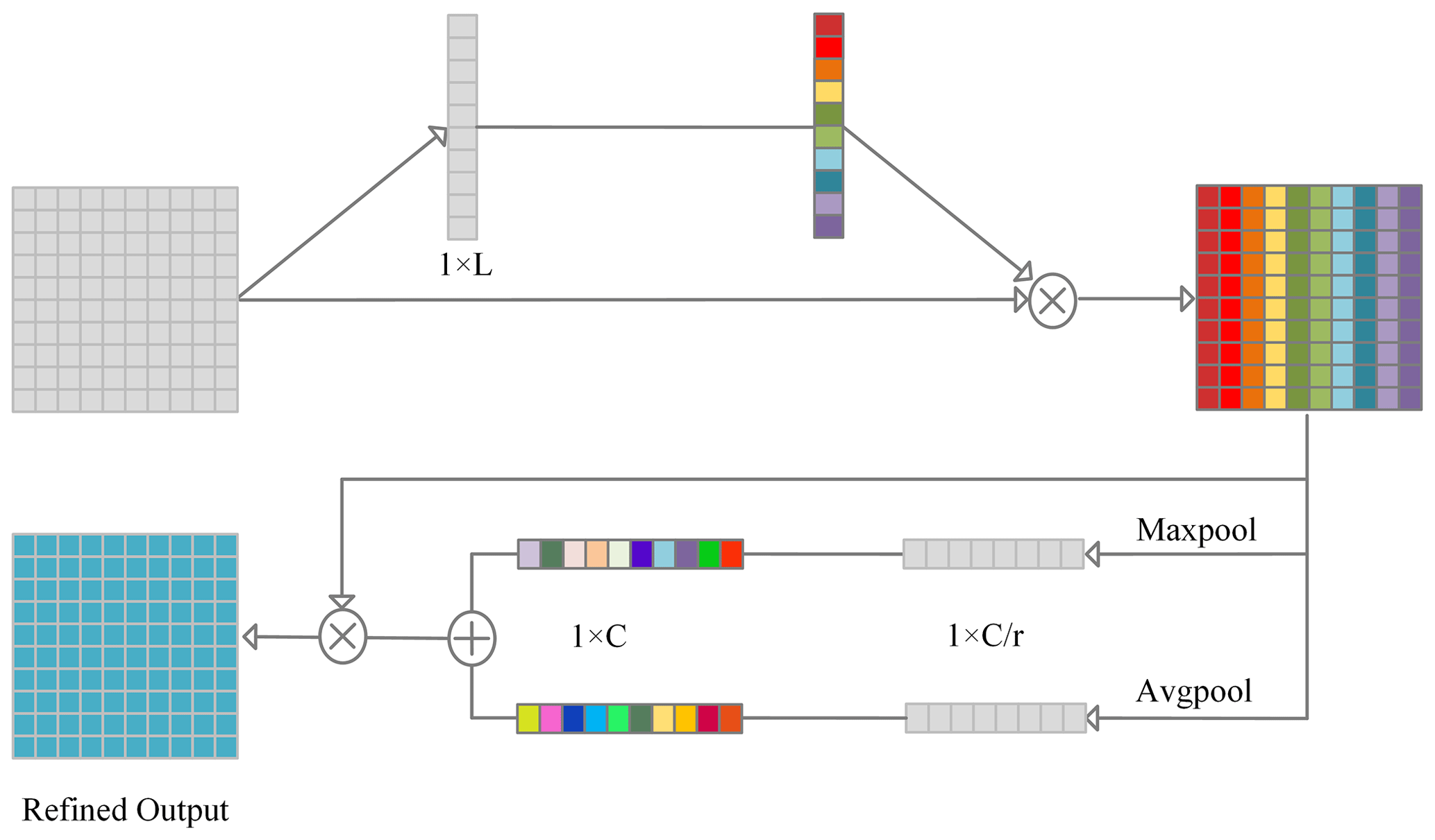
As for spatial information, we apply the convolutional operation to aggregate the compressed information from the channel dimensions (Roy et al., 2018).

The channel attention technique produces two feature maps with complementing global information through average and maximum pooling, respectively. Then, these two feature maps are then subjected to two separate convolution operations.

$$\begin{array}{}\text{(8)}& \begin{array}{rl}{C}_{\mathrm{out}}& =\mathit{\sigma }\left(W_{\mathrm{2}}\otimes \left(\mathit{\delta }\left(W_{\mathrm{1}}\otimes C_{max}\right)\right)\right.\\ & \left.+W_{\mathrm{2}}\otimes \left(\mathit{\delta }\left(W_{\mathrm{1}}\otimes C_{\mathrm{avg}}\right)\right)\right),\end{array}\end{array}$$

where C_max and C_avg are the global maximum pooling and global average pooling feature, W₁ and W₂ are the weights, δ is ReLU activation, σ denotes sigmoid activation, and ⊗ is convolution operation.

Input vectors can be optimized adaptively by DEM, to score the characteristics adaptively learned at various scales to enhance key information.

3.4 Fault detection framework

We present a framework for fault detection in Fig. 6. The framework adopts an end-to-end learning approach comprising four steps: signal acquisition and segmentation, model architecture development, model training workflow, and fault classification.

Figure 6 Fault detection framework.

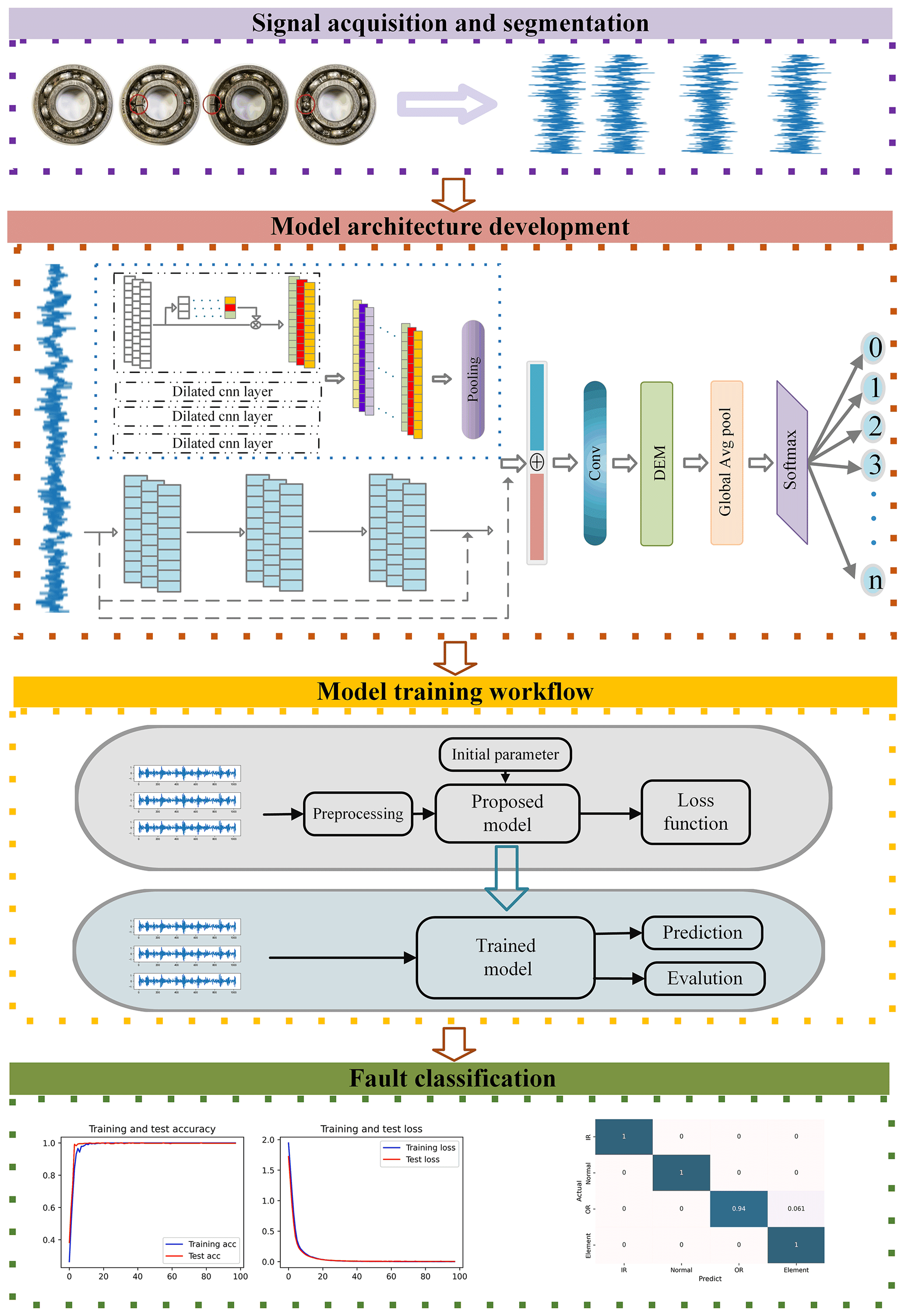
Step 1: signal acquisition and segmentation. The acquisition system collects the vibration data of mechanical components in varying states. Next, the original signal is divided into smaller units every 1024 data points, represented by

$$\begin{array}{}\text{(9)}& v=\left\{v_{\mathrm{1}},v_{\mathrm{2}},\mathrm{\cdots },v_n\right\}.\end{array}$$

Each segment of the vibration signal is tagged with one hot code during processing, so a separate bearing time-domain vibration dataset is represented as

$$\begin{array}{}\text{(10)}& \left\{\left(v_{\mathrm{1}},F_{\mathrm{1}}\right),\left(v_{\mathrm{1}},F_{\mathrm{1}}\right),\mathrm{\cdots }\mathrm{\cdots },\left(v_n,F_n\right)\right\}.\end{array}$$

If the number of data obtained are insufficient, data augmentation techniques are used to increase the sample size; otherwise, they are not necessary.

Step 2: model architecture development. Fault characteristics are extracted using multi-filter dilated and residual convolutional neural networks. The discriminative enhanced module picks characteristics from the extracted information that enhance the discriminating ones. Finally, we use the global average pooling layer to generate feature vectors and transfer them into softmax to output several fault sorts.

$$\begin{array}{}\text{(11)}& \mathrm{Softmax}\left(z_i\right)={\displaystyle \frac{e^{z_i}}{{\sum }_{j=\mathrm{1}}^n{e}^{z_j}}}\end{array}$$

Step 3: model training workflow. We feed the model our training data and then iteratively move forward through each model layer to get the prediction. According to the loss function, the loss between the prediction and the target is determined. The error is then back-propagated while modifying the training parameters to minimize the difference.

Step 4: fault classification. Input test data to the trained model. The detection model returns the fault category corresponding to the input signal.

4 Data description

4.1 CWRU dataset

The rolling bearing dataset from Case Western Reserve University (CWRU; http://csegroups.case.edu/bearingdatacenter, last access: September 2022) has been used extensively and has been considered a benchmark (Smith and Randall, 2015) in recent years.

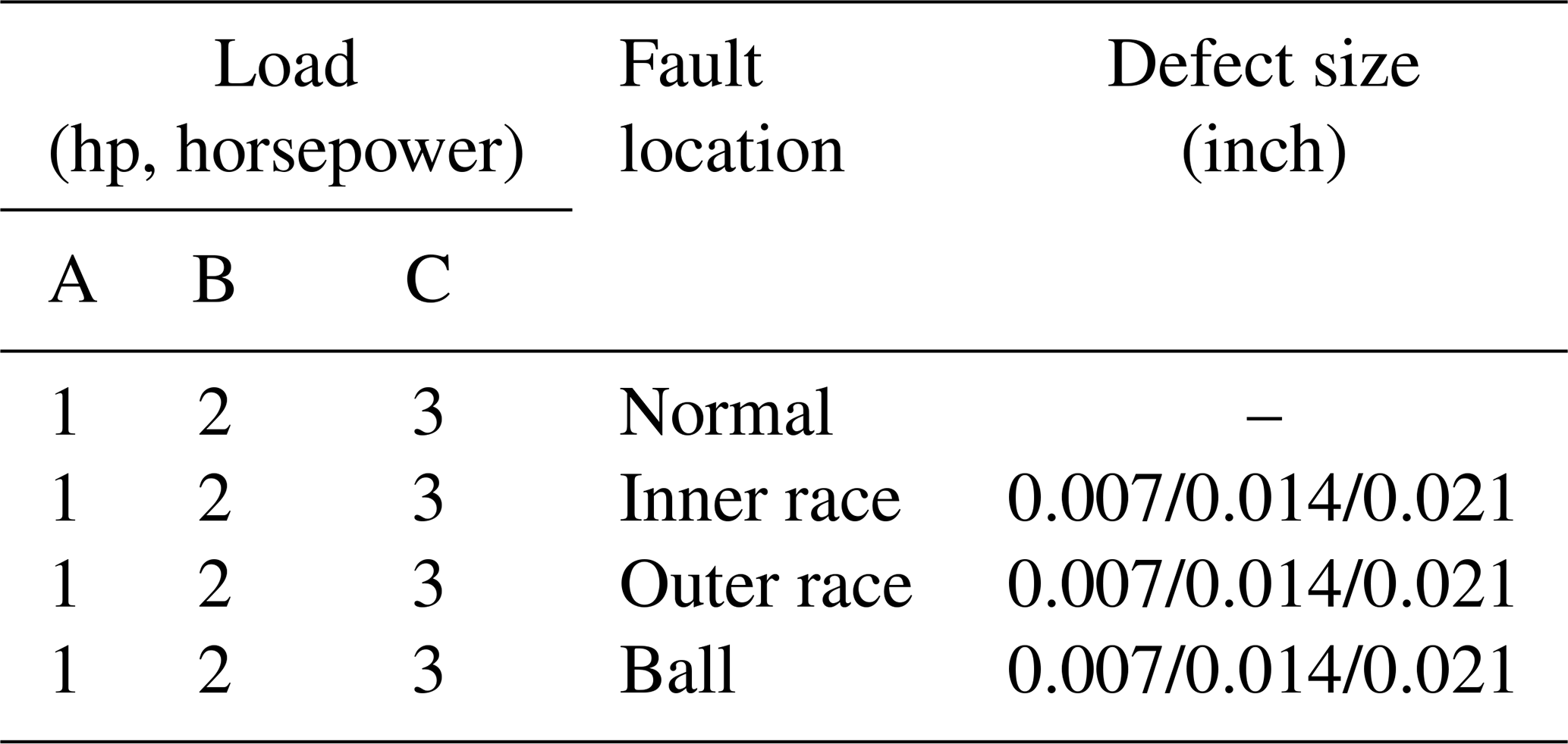
The vibration signals were collected from an accelerometer mounted on the drive end (DE) with a sampling frequency of 12 kHz. Three locations of failure were considered: inner-ring failure, outer-ring failure, and ball failure. Each position had three different fault diameters: 0.007, 0.014, and 0.021 in. Consequently, there were three fault types times three different fault diameters, along with normal operating conditions, totaling 10 fault types.

Datasets A, B, and C encompass vibration data from SKF 6205 bearings in three conditions: 1772 rpm (1 hp), 1750 rpm (2 hp), and 1730 rpm (3 hp), where bearing failures are seeded through electro-discharge machining, as shown in Table 1.

Table 1 Description of CWRU dataset.

4.2 JNU dataset

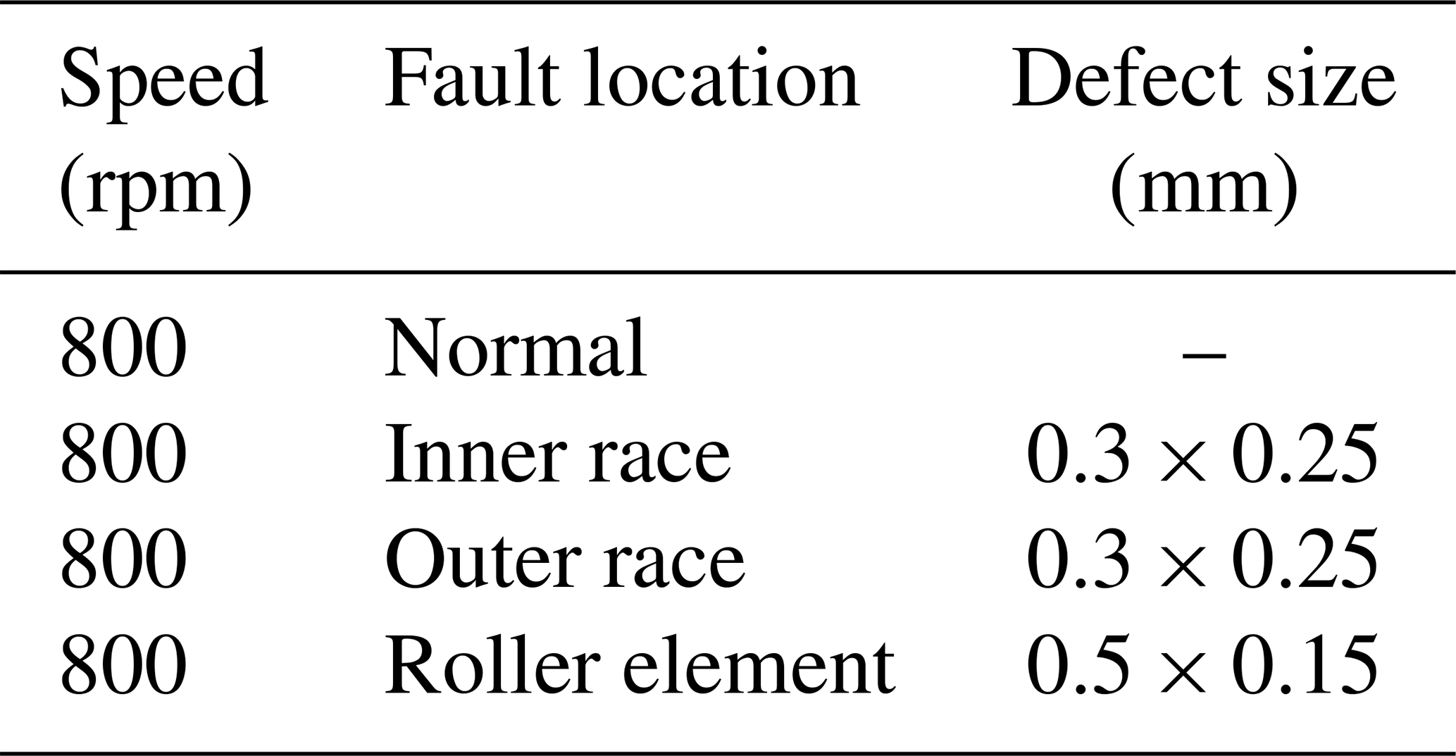
Two types of roller bearings (N205 and NU205) were used in Jiangnan University bearing datasets (Li et al., 2013). The sampling frequency is 50 kHz, and the sampling duration is 20 s. The vertical vibration signals of the bearings were measured in four states: normal, defective inner ring, defective outer ring, and defective roller element. The measurements were conducted independently using an accelerometer, amplified through a signal conditioner, and recorded. We utilize data obtained at 800 rpm; detailed information is outlined in Table 2.

Table 2 Description of JNU dataset.

4.3 Data augmentation

Training the model with a substantial volume of vibration signal data is critical to ensuring robust model fit. We have implemented an overlapping data augmentation technique (Zhang et al., 2017) to address the limited number of samples, as illustrated in Fig. 7. This method significantly increases the available training data, enhancing our model's performance.

Figure 7 Overlapping data augmentation.

5 Experimental validation and results

In this section, we validate various scenarios and analyze the corresponding outcomes.

5.1 Experimental setting

The training set of A, B, and C comprises 2000 samples, with a separate validation set and test set, each containing 300 samples.

We choose cross-entropy loss as the loss function to measure performance, and its mathematical formula is as follows:

$$\begin{array}{}\text{(12)}& H(p,q)=-\sum _{x}p\left(x\right)\log q\left(x\right),\end{array}$$

where p(x) indicates the true probability distribution and q(x) is the predicted probability distribution.

In order to accelerate the training speed while avoiding falling into local optimal points, this paper uses the Adam stochastic optimization algorithm for training, which can dynamically adjust the learning rate of different parameters by iterating the weights according to the training data. The dropout rate during training is 0.3.

The framework used for the experiments is TensorFlow 2.6.0, running on a computer with an Intel i5 11400 CPU and an RTX3060 12 GB GPU. To better train the model in the TensorFlow framework, callback functions, early stop, and exponential decay learning rate scheduler are utilized to ensure optimum generalization performance.

5.1.1 The effect of dilation rates

If the kernel size of the filter is ks and the dilation rate is d, then the equivalent convolution kernel size ks^′ is

$$\begin{array}{}\text{(13)}& {\mathrm{ks}}^{\prime }=\mathrm{ks}+(\mathrm{ks}-\mathrm{1})\times (d-\mathrm{1}).\end{array}$$

When the dilation rate exceeds 1, the receptive field of the convolution kernel can be enlarged based on Eq. (13). By configuring a set of dilation rates to establish multiple receptive fields, the module can capture signal features across a broad range of scales.

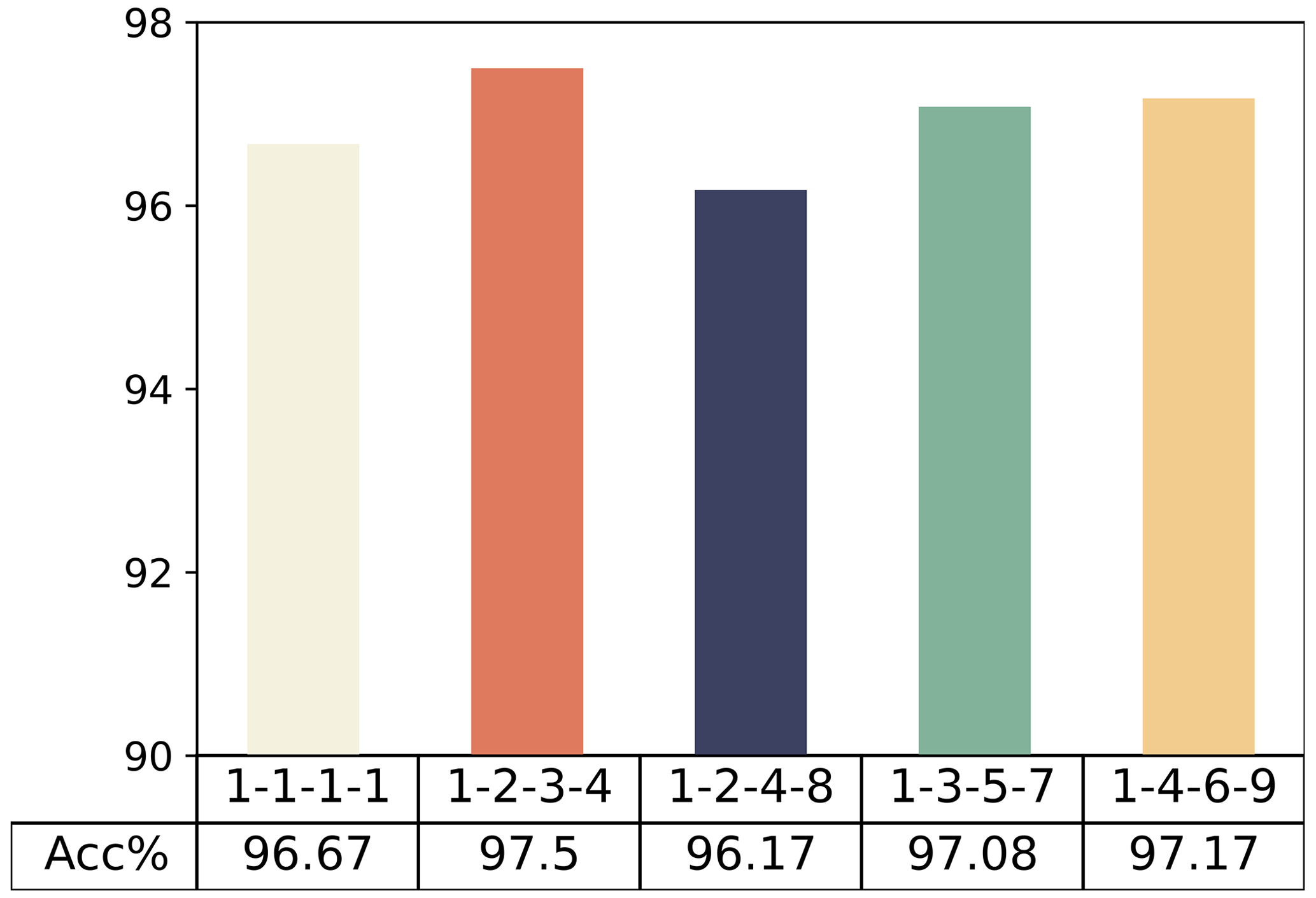
To find the optimal combination, we attempted to validate sets with various rates. The standard convolution combination is ($\mathrm{1},\mathrm{1},\mathrm{1},\mathrm{1}$), while the other combinations tested include ($\mathrm{1},\mathrm{2},\mathrm{3},\mathrm{4}$), ($\mathrm{1},\mathrm{2},\mathrm{4},\mathrm{8}$), ($\mathrm{1},\mathrm{3},\mathrm{5},\mathrm{7}$), and ($\mathrm{1},\mathrm{4},\mathrm{6},\mathrm{9}$).

Validation was conducted using training set C, test set A, and test set B, while keeping all other variables constant and with an initial reduction ratio of 16. In the comparison of sets of dilation rates in Fig. 8, the combination of ($\mathrm{1},\mathrm{2},\mathrm{3},\mathrm{4}$) achieved the best results with an average diagnostic accuracy of 97.5 %, indicating it has the strongest feature extraction performance.

Figure 8 Results of different sets of dilation rates.

5.1.2 The effect of reduction ratios

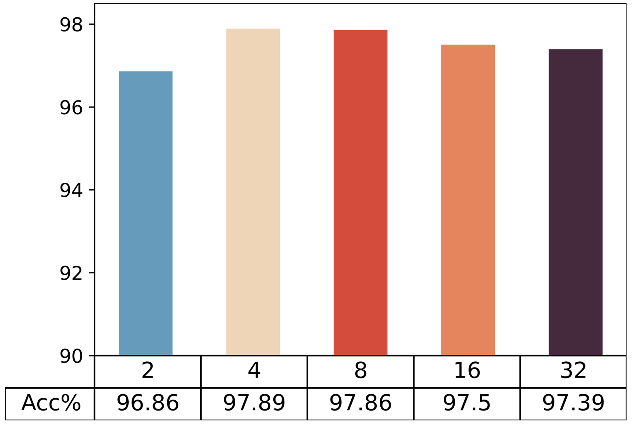
The attention mechanism enhances the model's ability to discern fault features by adjusting weights, and the reduction ratio stands out as a crucial parameter. This ratio reduces computational complexity by decreasing the number of input channels, aiding the model in efficiently capturing inner correlations. An appropriate reduction ratio helps regulate weight ranges, concentrating on the most pertinent elements in the input and enhancing the model's expressiveness. Typically, the reduction ratio is a positive integer, with common values being 2, 4, 8, 16, etc. Comparative diagnostic results for the model with different reduction ratios are presented in Fig. 9. The optimal ratio for this diagnostic task is 4.

Figure 9 Results of different reduction ratios.

5.2 Performance under different workloads

Due to production requirements and unforeseen external environmental factors, machines often operate under varying conditions, including speed, load, and temperature. These fluctuations impact the vibration frequency and amplitude of signals captured by accelerometers, leading to notable differences in signal characteristics. Consequently, these changes introduce interference, affecting the accuracy of classification. The variation in data distribution caused by these fluctuations significantly impacts the overall generalization performance of fault diagnosis models.

Figure 10 Results of different workloads.

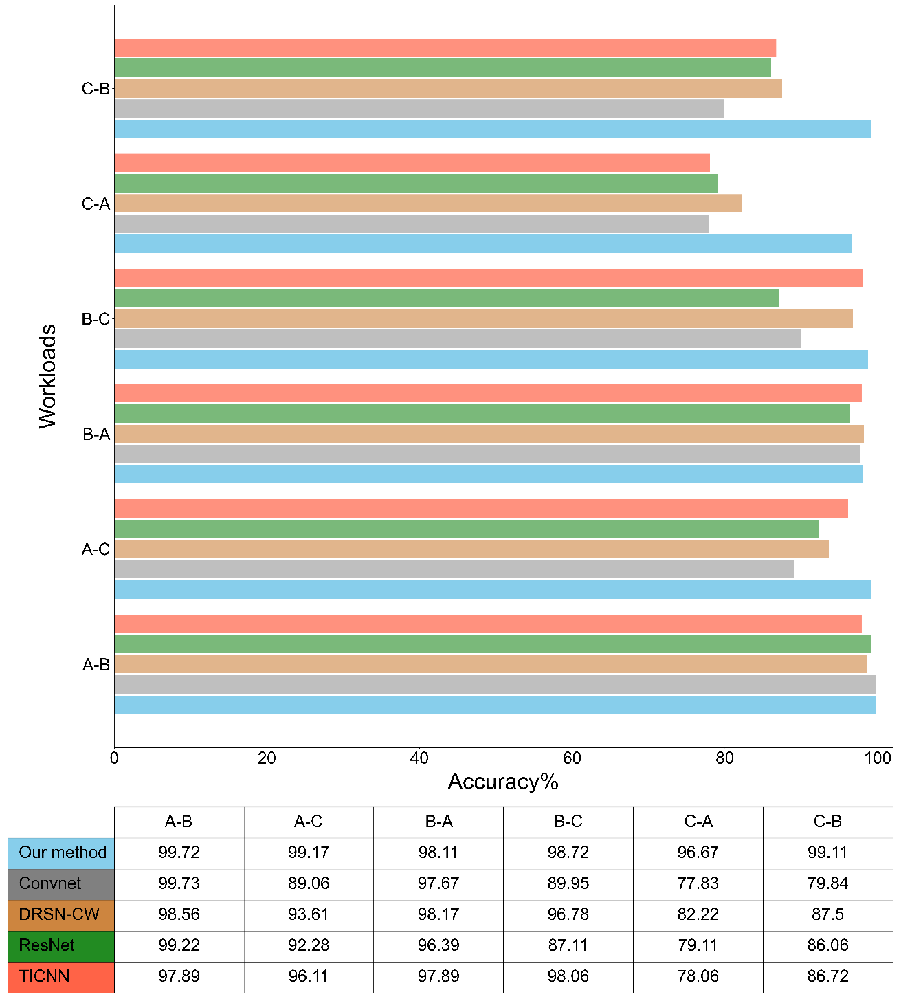
It requires good robustness of the diagnostic model to adapt to various changes in operating conditions. In the following section, the adaptability of the models, i.e., the proposed method, ConvNet, DRSN-CW (Zhao et al., 2019), ResNet, and TICNN (Zhang et al., 2018), is tested under different workloads. The validation method involves training the model on a specific workload and then applying it to test sets from a different workload, with results presented in Fig. 10.

TICNN, configured with a wide kernel size of 64, consistently achieves accuracy above 96 % for the initial four workloads. However, a substantial decline in diagnostic accuracy is observed for C–A and C–B, plummeting to 78.06 % and 86.72 %, respectively. In contrast to TICNN, ConvNet employs small kernels in each layer. Notably, ConvNet gains better performance exclusively in the A–B scenario. This observation demonstrates that a wide kernel is instrumental in extracting crucial vibrational features from the signal while suppressing spurious feature interference.

DRSN-CW embeds soft thresholding within the architecture, achieving an average diagnostic accuracy of 96.78 % for the initial four loads. Nevertheless, it incorporates a limited number of filters, potentially impeding the extraction of intricate feature representations and diminishing the capacity to distinguish various fault features effectively. DRSN-CW can just achieve more than 80 % diagnostic ability under C–A and C–B.

ResNet uses the same filter quantity as DRSN-CW in the B–C scenario but falls behind DRSN-CW by over 9 %, indicating that incorporating soft thresholding aids the DRSN-CW model in learning more robust feature representation. Our model achieves the best average diagnostic results in multi-load domain adaptation tasks, demonstrating that our model in this study can learn more discriminative features about these defects and enhance the model's robustness in complex scenarios.

Figure 11 t-SNE visualization results.

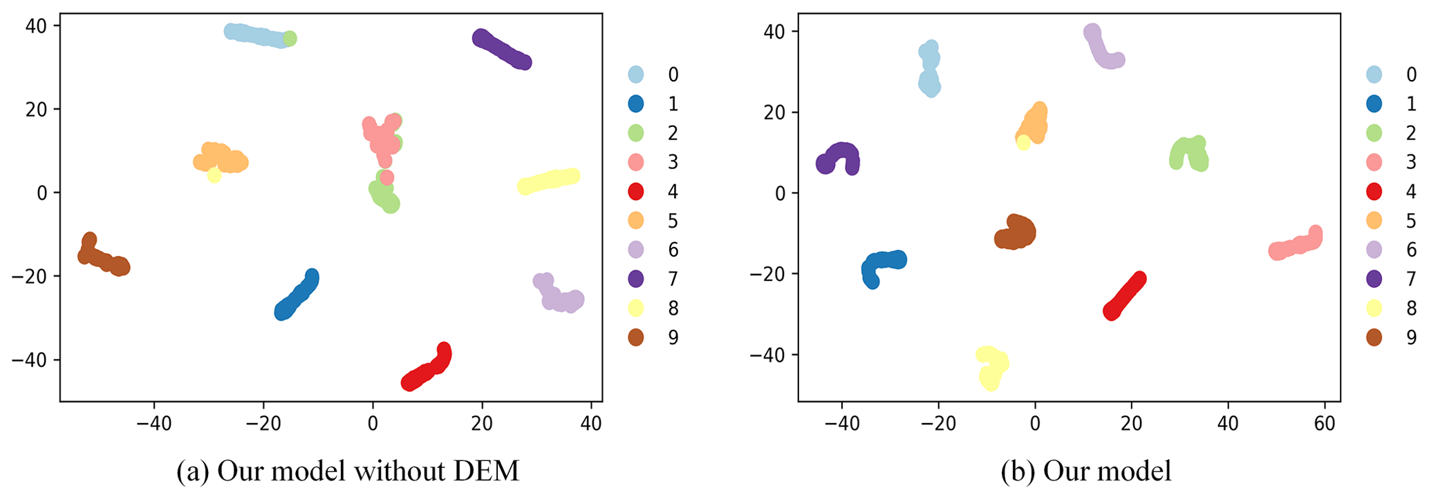
To intuitively observe the final classification results, we employ the t-SNE algorithm (Van Der Maaten and Hinton, 2008) to map abstract features under the A–C workload into a comprehensible geometric plane, as illustrated in Fig. 11. Different colors represent various bearing failures, visually demonstrating the degree of separation among failure characteristics. The model equipped with the DEM module exhibits higher separation when distinguishing between different classes of samples, underscoring its ability to prioritize fault-relevant information and enabling more accurate classification decisions.

5.3 Performance with the JNU dataset

To assess the generalizability of the proposed model, validation experiments were performed using the JNU dataset. In order to gain a deeper understanding of the model's diagnostic capabilities, we introduced the confusion matrix to provide a detailed representation of the model's performance within each fault category.

Figure 12 Comparison of confusion matrices.

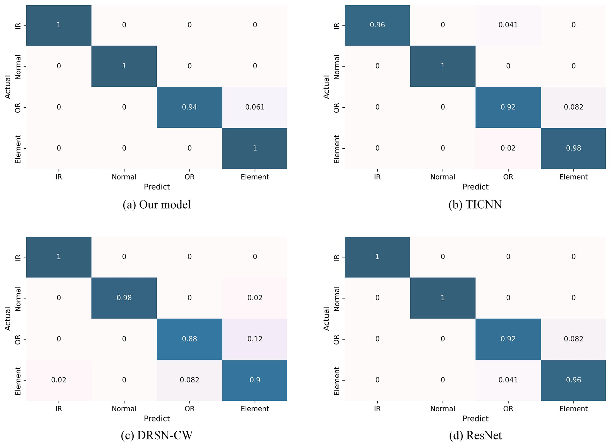
As illustrated in Fig. 12, the four confusion matrices represent the diagnostic results of our model, TICNN, DRSN-CW, and ResNet. In the case of outer-race fault detection, DRSN-CW exhibits a 12 % probability of erroneously classifying such faults as roller element faults. Regarding roller element damage diagnosis, this model encounters a 2 % chance of confusion with inner-race faults and an 8.2 % likelihood of incorrect classification as outer-race faults. TICNN accurately predicts all samples in the healthy state; however, it trails our model by 4 % in diagnosing inner-race faults and lags by a margin of 2 % in the other two fault scenarios. ResNet shows commendable accuracy in diagnosing faults in inner-race and healthy-state samples, with a 100 % correct prediction rate in these categories. Nonetheless, its diagnostic accuracy diminishes by 8 % and 4 % for the remaining fault types.

Our proposed model excels in superior diagnostic proficiency across a spectrum of bearing faults and degrees of damage, accurately detecting all instances of faults in three scenarios and attaining a 94 % accuracy in identifying outer-race faults. The experimental outcomes demonstrate that our model achieves a convincing performance with the JNU dataset, substantiating its robust generalizability.

6 Conclusion

This study offers a novel framework based on convolutional neural networks for detecting industrial bearing faults. The framework incorporates dilated convolution, residual convolutional neural network, and attention mechanisms to gain rich fault feature representations and adaptively enhance key information. It is able to extract multi-scale features from nonlinear vibration signals to overcome the limitations of single-structure convolutional neural networks' weak flexibility and extraction capacity. Multiple types of experimental validation are performed on bearing datasets. The experimental results show that the proposed model considerably exceeds traditional CNNs in feature learning and classification ability.