the Creative Commons Attribution 4.0 License.
the Creative Commons Attribution 4.0 License.
 | 08 Aug 2022
Autonomous vehicle trajectory tracking lateral control based on the terminal sliding mode control with radial basis function neural network and fuzzy logic algorithm
Binyu Wang
Yulong Lei
Yao Fu
Xiaohu Geng
This paper will study a trajectory tracking control algorithm for electric vehicles based on a terminal sliding mode controller. First, a 3 degrees of freedom nonlinear vehicle model and a controller-oriented 2 degrees of freedom vehicle model are established. The preview time is adaptively adjusted based on the preview model. Then, the vehicle trajectory tracking controller, which uses the terminal sliding mode algorithm, is designed. The radial basis function (RBF) neural network algorithm is used to approximate the system variable parameters in the control model online. At the same time, fuzzy logic is used to control the gain parameters of the controller to reduce the chattering of the control system. Finally, the designed controller is verified by simulation. The maximum deviation of path tracking under different speeds is 0.6 m, and the target path can also be well followed under different road friction coefficients. The simulation results show that the controller designed in this paper can effectively carry out the vehicle trajectory tracking and lateral control and reduce the chattering to a certain extent.
- Article
(6513 KB) - Full-text XML
- BibTeX
- EndNote


In recent years, autonomous technology has become the critical research direction of vehicle technology. One of its core technologies is to control technology. The control system determines all the actions of autonomous vehicles, and the excellent performance controller is the basis for autonomous technology. Trajectory tracking is an integral part of the autonomous vehicle, and better tracking capabilities are the basic needs of autonomous vehicles (Gonzalo et al., 2020; Xiong et al., 2020). However, because the vehicle system has the characteristics of strong nonlinearity and high coupling, its dynamic model is very complex and cannot be accurately represented. Therefore, trajectory tracking control is always a major difficulty in realizing autonomous driving technology.
The trajectory tracking of autonomous vehicles attracts a wide range of attention from many scholars and proposes several control methods to achieve trajectory tracking. Abatari and Tafti (2013) designed a fuzzy proportional–integral–derivative (PID) controller for the path following of car-like mobile robots. Zhang et al. (2019) used the Takagi–Sugeno fuzzy control method to study the steering control problem of vehicle trajectory tracking with uncertain parameters. Boumediene et al. (2020) carried out tracking control on the established 3 DOF (degrees of freedom) model by combining the adaptive neural fuzzy reasoning system and particle swarm optimization algorithm. To improve the stability of autonomous vehicles, Yuan et al. (2019) track the trajectory based on the model predictive control algorithm by increasing the dynamic constraints of the center of mass, acceleration, and tire side angle. Liang et al. (2017) applied model predictive control to deal with low-speed trajectory tracking to ensure the reasonable safety of autonomous vehicles. Zhou et al. (2019) designed the electromechanical coupling dynamic trajectory tracking controller based on the model predictive control algorithm. Li et al. (2020) proposed a linear predictive lateral control method. The lateral force of the front tire was selected as the control input. The friction between the front and rear tires was used as the safety constraint of the predictive controller for the stability control of vehicle path tracking at high speed. Wang et al. (2018) proposed a new model predictive control strategy based on the adaptive cost function, which reflects different requirements under different road classes and friction coefficients. The strategy is applied to the longitudinal control of intelligent vehicles.
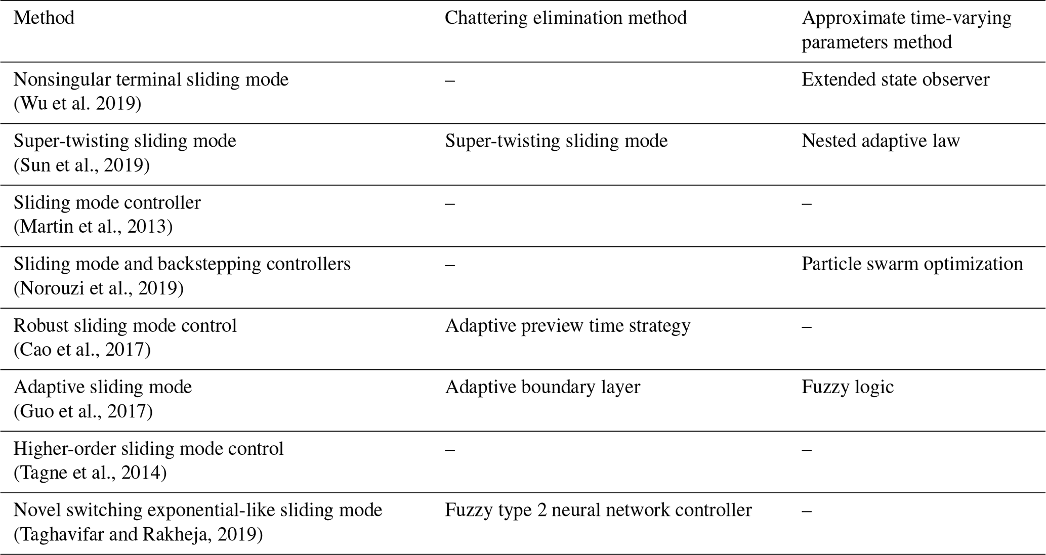
The sliding mode control (SMC) algorithm is widely used in nonlinear control systems due to its characteristics. SMC has strong robustness to strong nonlinearity, external disturbance, and parameter uncertainty and disturbance caused by complex driving conditions of autonomous vehicles (Wu et al., 2019). In addition, the SMC controller allows the vehicle to converge quickly to the path (Sun et al., 2019). Martin et al. (2013) designed a trajectory tracking controller using a sliding mode control algorithm based on the kinematic model. Based on the 2 DOF vehicle model, Norouzi et al. (2019) combined the sliding mode controller with the back-stepping controller to control the steering. Cao et al. (2017) designed a robust sliding mode control steering controller with an adaptive preview time strategy, which can carry out path tracking and avoid significant acceleration caused by adaptive preview time strategy during trajectory tracking. The most critical sliding mode control problem is the chattering caused by the sliding surface switching. In recent years, many methods have been proposed to eliminate chattering. However, reducing or eliminating chattering is still the key to the design of a sliding mode controller (Tagne et al., 2014; Guo et al., 2017; Taghavifar and Rakheja, 2019).
The objective of this paper is the trajectory tracking control of vehicles. The contribution of this paper is as follows: (1) an autonomous vehicle trajectory tracking controller based on the terminal sliding mode control is designed. (2) Because the control system contains state-dependent, time-varying parameters which cannot be known in advance, it is necessary to approximate them, and the approximation value is used as the design basis of the controller. The radial basis function (RBF) neural network controller is designed to approximate the time-varying parameters. (3) To reduce the chattering of the controller, the fuzzy algorithm is used to control the gain of symbol function control. (4) The simulation analysis of the designed controller is carried out under the double lane-shifting condition to verify its effectiveness, and the influence of different vehicle speeds and different road adhesion coefficients on the controller is studied. The structure design of this paper is as follows. Section 1 introduces the current research status of scholars and the research content of this paper. Section 2 establishes the vehicle dynamics model and tire model. Section 3 establishes the driver preview model, designs the controller, and conducts stability analysis for the designed controller. Section 4 carries out the simulation analysis of the controller, conducts the simulation verification of the controller designed in this paper under the condition of the double line change, and compares the control effect between the controller designed in this paper and the traditional terminal sliding mode controller. Section 5 is the conclusion of this paper.
An accurate vehicle dynamics model can accurately reflect the kinematic and dynamic characteristics of the vehicle, which is the basis of vehicle controller design. In this paper, from the realization of the control goal of autonomous vehicle steering, a dynamic model that can reflect the lateral characteristics of the vehicle is established. The established model needs to ensure that the response of the vehicle model can be similar to or consistent with the actual vehicle and meet the requirements of the trajectory tracking lateral controller designed in this paper. Therefore, this section established the vehicle model with 3 DOF, the controller-oriented model with 2 DOF, and the Dugoff tire model (Dugoff et al., 1970).
Table 1Various SMC techniques for trajectory tracking and their control strategies.
2.1 Vehicle model with 3 DOF
In this paper, a 3 DOF nonlinear model including longitudinal, lateral, and yaw motion is established by using a simplified model. The 3 DOF nonlinear model is shown in Fig. 1. XOY is the geodetic reference frame, and xoy is the vehicle reference frame. a is the distance from the center of mass to the front axis, and b is the distance from the center of mass to the rear axis. tf is the front wheel tread, tr is the rear wheel tread, ω is the yaw rate, β is the sideslip angle, V is the vehicle's speed, u is longitudinal velocity, and v is lateral velocity. Fxi () is the longitudinal force on the four tires, Fyi ( is the lateral force on the four tires, αi () is the sideslip angle of the four tires, and δ is the steering angle.
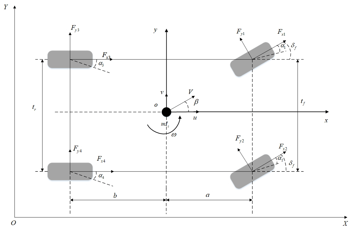
Meanwhile, the following assumptions are made: (1) ignoring the influence of the steering operating mechanism, the front wheel angle is directly taken as input, and the left and right front wheel angles are assumed to be equal. (2) The effect of the suspension system is not considered, only the translational motion of the vehicle along the x axis and y axis is considered, and the influence of pitch motion, vertical motion, and roll motion of the vehicle is not considered, and (3) the effects of aerodynamics are ignored. The dynamic equations of the nonlinear vehicle model are as follows (Feng et al., 2020):
where X and Y represent the vehicle's coordinates with the geodetic coordinate system as the reference frame, ψ is the vehicle's heading angle, m is the vehicle's mass, and Iz is the moment of inertia of the vehicle around the z axis.
2.2 Tire model
In this paper, the Dugoff tire model (Dugoff et al., 1970) is used to calculate the longitudinal and lateral forces of the tire. For each wheel, the longitudinal and lateral forces acting on the tire can be expressed as follows:
where
The following formula calculates each tire sideslip angle, vertical load, and slip rate (Feng et al., 2020):
where μi is the tire–road friction coefficient, λi is the longitudinal slip ratio, cx is the longitudinal stiffness of tire, cy is the lateral stiffness of tire, ε is the velocity influence factor, Fzi is the vertical tire load, R is the wheel rolling radius, ωi is the wheel rolling angular velocity, vi is the speed of the wheel center, ax and ay are the longitudinal and lateral acceleration, h is the height of the center of mass, and l is the wheelbase.
2.3 Controller-oriented 2 DOF model
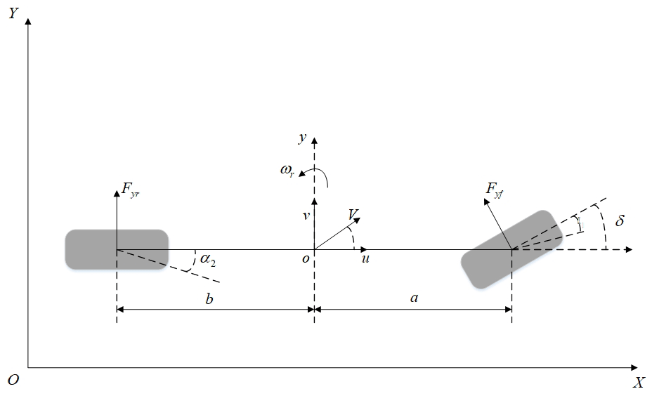
Since the lateral and yaw motions are mainly involved in the path-tracking control process, to reduce the calculation amount, a single wheel is used to replace the two wheels on the axle, so as to simplify the four-wheel vehicle into a monorail vehicle model. At the same time, it is assumed that the relationship between the tire sideslip force and the sideslip angle is linear. The 2 DOF vehicle dynamics model is shown in Fig. 2, and the dynamic equation is as follows (Feng et al., 2020):
where cf is the front wheel lateral stiffness, cr is the rear wheel lateral stiffness, and ω is the yaw rate. The coordinate transformation formula between the geodetic and vehicle coordinate systems is the same as the 3 DOF model, so it will not be repeated.
Equation (9) can be expressed as the equation of state, as follows:
where
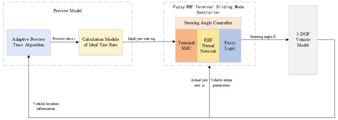
The structure of the controller is shown in Fig. 3. First, the optimal preview time is obtained according to the preview time adaptive algorithm, and the optimal preview distance and expected yaw rate are calculated. Then, the yaw rate error is taken as the control input, and the steering wheel angle output by the controller is input into the 3 DOF vehicle model. Finally, the vehicle model feeds back the vehicle state parameters such as yaw rate and yaw velocity to the controller to achieve the closed-loop control.
3.1 Preview model construction
The vehicle will encounter a variety of emergencies in the running process. Therefore, in the process of vehicle driving, the path ahead can be assessed, and the corresponding decision can be made in advance, so that the vehicle can better track the desired trajectory. The trajectory tracking control method proposed by Macadam (2003) has been widely applied in the longitudinal and lateral control of automobiles. The basic idea of the optimal preview driver model is to establish the optimal index function according to the position of the road ahead, the vehicle state, and the lateral position deviation in the preview time, and the optimal steering angle is obtained to control the vehicle to track the ideal trajectory.
In general driver models, the preview time is set as a fixed value, but under the conditions of high speed, complex trajectory, and road width constraints, driver models with fixed preview time often find it challenging to complete driving tasks. Therefore, to improve the adaptability of the driver model, the preview time is adaptively controlled. A different preview time tp is selected, and the adaptive optimization function of the preview time is designed according to the trajectory deviation, boundary distance, yaw angle deviation output by vehicle model, and pavement model in time t1. The appropriate preview time is selected according to the optimization function. It is controlled according to the preview time at this time. The optimization functions are designed as follows:
-
Trajectory deviation optimization function:
-
Boundary position optimization function:
-
Yaw angle deviation optimization function:
-
Dynamic response time optimization function:
where yt and ye are the target trajectory and the predicted trajectory, t1 is the model prediction time, Δ is the distance from the centerline to the boundary, and ψr and ψd are the yaw angle and the target heading angle at this time. tp is the previewing time used for the calculation, and T′ is the time associated with vehicle steering response characteristic.
The trajectory deviation optimization function calculates the trajectory deviation within the preview time. The longer the preview time, the greater the trajectory deviation. The purpose of the boundary position optimization function is to constrain the vehicle at a position far from the road boundary through the optimization function to ensure the safe passage of the vehicle. By calculating the deviation between the yaw angle and the target heading angle at the current moment, the yaw angle deviation optimization function ensures that the difference between the vehicle direction, and the target trajectory tangent direction at the beginning of the next stage is slight. This reduces the difficulty of steering control in the next stage. The longer the preview time, the easier it is for the vehicle to maintain stability in a particular range, but the prediction accuracy will deteriorate. The dynamic response time optimization function calculates the difference between the preview time and the vehicle steering response time, ensuring calculation accuracy while optimizing the preview time. According to Eqs. (11)–(14), the optimization objective function is as follows:
where w1, w2, w3, and w4 are the weight coefficient. The selection of different weight coefficients corresponds to different driving styles. By optimizing the algorithm, the appropriate preview time t can be obtained. After calculating the optimal preview time, the preview distance can be calculated according to the current velocity, and the following formula can calculate the target yaw rate (Chen et al., 2016):
3.2 Design of terminal sliding mode controller
According to Eq. (10), the state equation of the control system in this paper can be expressed as follows:
where , and D(t) is the uncertainty of the system and external interference, which can be represented as follows:
The control input is the yaw rate error, which can be expressed as follows:
where ωr is the real yaw rate, and ωd is the target yaw rate. The terminal sliding mode surface function is designed as follows:
where c is the control parameter, and c>0.
Combining the above equation, the control law can be designed as follows:
3.3 Design of the RBF neural network
In Eq. (20), there are time-varying parameters in f(ω), so the neural network method can be used for the online approximation of f(ω). The RBF neural network has a good generalization ability, simple network structure, and universal approximation characteristics, when compared with BP neural network. It can avoid unnecessary and lengthy calculations and realize online tuning, so this paper selects the RBF network to achieve an adaptive approximation of system parameters. The algorithm of the RBF neural network is as follows:
where x is the network input, cj is the central point coordinate of the Gaussian basis function of the jth neuron in the hidden layer of the network, bj is the width of the Gaussian basis function of the jth neuron in the hidden layer, hj is the hidden layer output, w∗ is the ideal weight of RBF network, y(t) is the RBF network output, and ε is the network approximation error. The RBF network structure is 2–5–1.
For the RBF network in this paper, we take the control input e and its derivative as the network input, that is, . The number of hidden layers in the network is five, and the network output is the approximate value of f(ω). So, the following can be obtained:
where w is the real weight of the RBF network. In order to adjust the weight adaptive, the following adaptive law is designed:
The RBF network for online approximation of time-varying parameters as shown in Fig. 4.

Figure 4 shows that the RBF neural network designed in this paper is effective in approximating time-varying parameters, and the error between the approximation value and the actual value is small, which can be used for controller design. By substituting the designed RBF network output into Eq. (20), the adaptive sliding mode control law of RBF network can be obtained as follows:
3.4 Design of switching gain fuzzy controller
The chattering of the SMC is mainly caused by the sign function sign(s). Generally, the sign function is changed into saturation to reduce the chattering. In this paper, the fuzzy control method based on the gain is used to reduce the chattering of the sliding mode control system.


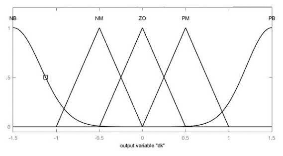
The actual sliding mode movement trend is shown in Fig. 5. According to the figure, the fuzzy rule can be set as follows: (1) when , the system state point is approaching the sliding mode surface, and the value of D should increase. (2) When , the system state point is far away from the sliding mode surface, and the value of D should decrease. We know that D is a positive constant. Therefore, ΔD is selected as the output of the fuzzy system, and then the value of D is estimated by the integral method. The input itself already contains the change and rate of change of the switching function s, and the rate of change of is not easy to calculate, so only is selected as the system input. Based on the fuzzy rule, the input and output fuzzy set of the system can be defined as follows. The domain determination and membership function selection are shown in Figs. 6 and 7.
The fuzzy rules are designed as follows:
-
Rule 1 – if is PB, then ΔD is PB.
-
Rule 2 – if is NM, then ΔD is NM.
-
Rule 3 – if is ZO, then ΔD is ZO.
-
Rule 4 – if is PM, then ΔD is PM.
-
Rule 5 – if is NB, then ΔD is NB.
The corresponding results of the input and output are obtained according to the fuzzy rules, and the upper boundary condition of is estimated by the integral method.
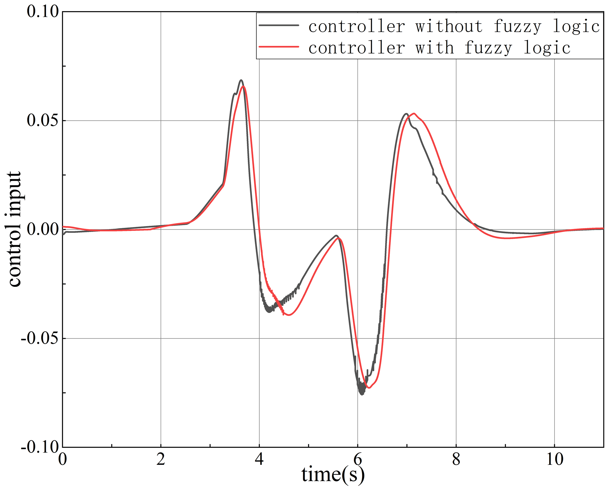
Figure 8 shows the effect of the fuzzy logic control algorithm on reducing chattering. It can be seen from Fig. 8 that the fuzzy logic algorithm has a pronounced effect on the elimination of chattering. In the whole control process, the control input chattering of the controller with the fuzzy logic algorithm is much smaller than that of the controller without the fuzzy logic algorithm. It is proved that the fuzzy logic controller designed in this paper is effective at eliminating chattering of the sliding mode controllers.
So far, the design of the fuzzy RBF neural network terminal sliding mode controller is completed. The control law of the controller designed in this paper is summarized as follows: is the approximation value of time-varying parameters which approximate by the RBF neural network algorithm, and is the estimated value of control gain by the fuzzy logic algorithm.
3.5 Stability analysis of the algorithm
According to Eq. (20), we can obtain the following:
We then substitute Eq. (25) into the above equation.
where .
The Lyapunov function is designed as follows:
Taking the derivative of this equation, we have the following:
It can be obtained by substituting Eq. (24) into Eq. (31) as follows:
where . Since the approximation error of the RBF network εf is very small, can be obtained as long as is guaranteed, so that the system is asymptotically stable. And when s→∞, L→∞, the system must be asymptotically stable in a large range, while ensuring that it is asymptotically stable.
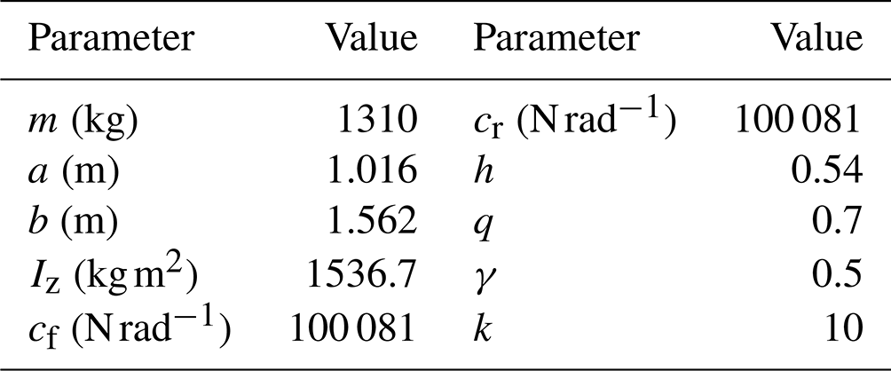
In order to verify the effectiveness of the designed terminal sliding mode controller, trajectory tracking control under different speeds and limit conditions and different control methods are compared and simulated. Part of the relevant parameters of the vehicle model and controller are shown in Table 1. The route of the double shift line condition is selected for the prescribed route.
First, the influence of speed on the designed sliding mode controller was observed, and the car was allowed to track the specified double line movement condition at the speed of 10, 15, and 20 m s−1, respectively. The simulation results are shown in Figs. 9–12.

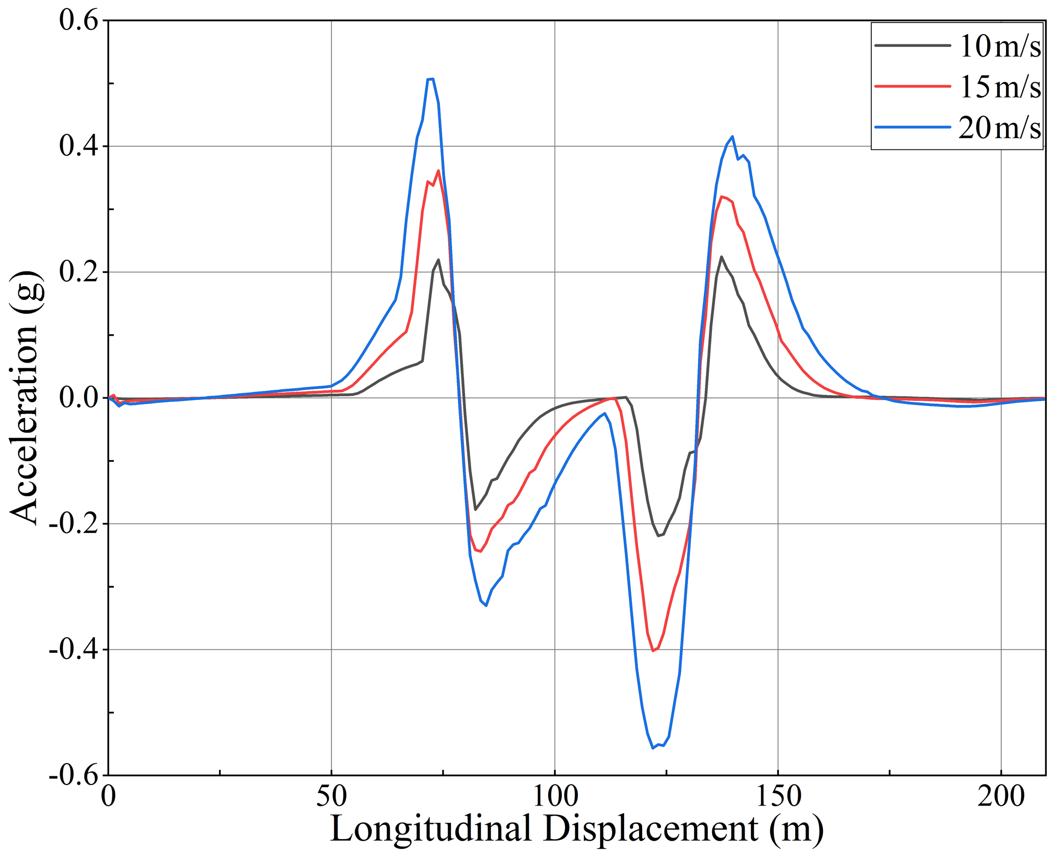
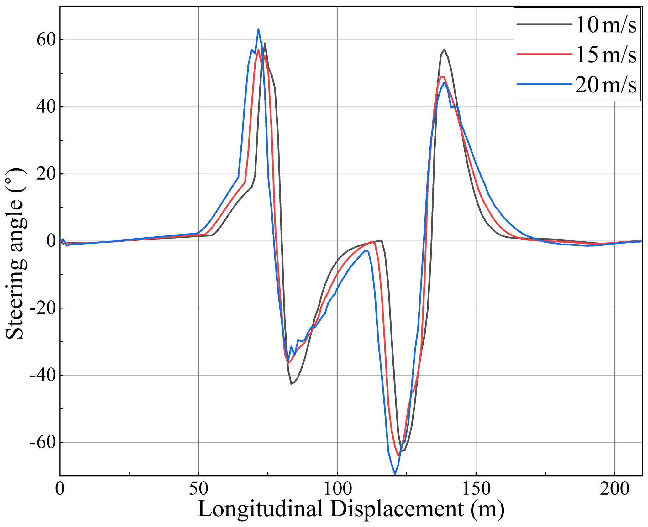
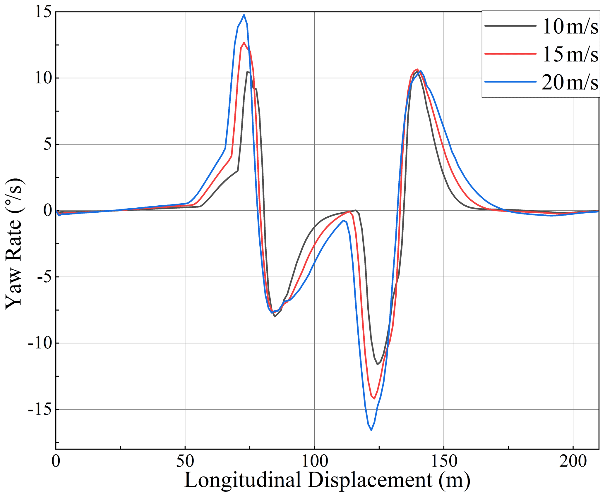
It can be seen from Fig. 9 that, under three different speed conditions, the designed controller can ensure good tracking of the pre-set track at three different speed conditions. With the increase in speed, the lateral deviation of the vehicle increases gradually, but it can still guarantee the basic consistency with the pre-set track direction. With the increase in vehicle speed, the trend of vehicle lateral acceleration, steering wheel angle, and yaw rate is basically similar, with only a numerical increase. Although there is some chattering, the fluctuation is slight, which meets the lateral control requirements of the vehicle. The above simulation results can verify that the designed controller can meet the requirements of vehicle trajectory tracking and lateral control at different speeds.
In order to verify the effectiveness of the controller under low road friction coefficient, the speed was set to 20 m s−1, and the double line change was simulated on the road surface with road friction coefficients of 0.8, 0.6, 0.4, and 0.2. The simulation results are as shown in Figs. 13–16.
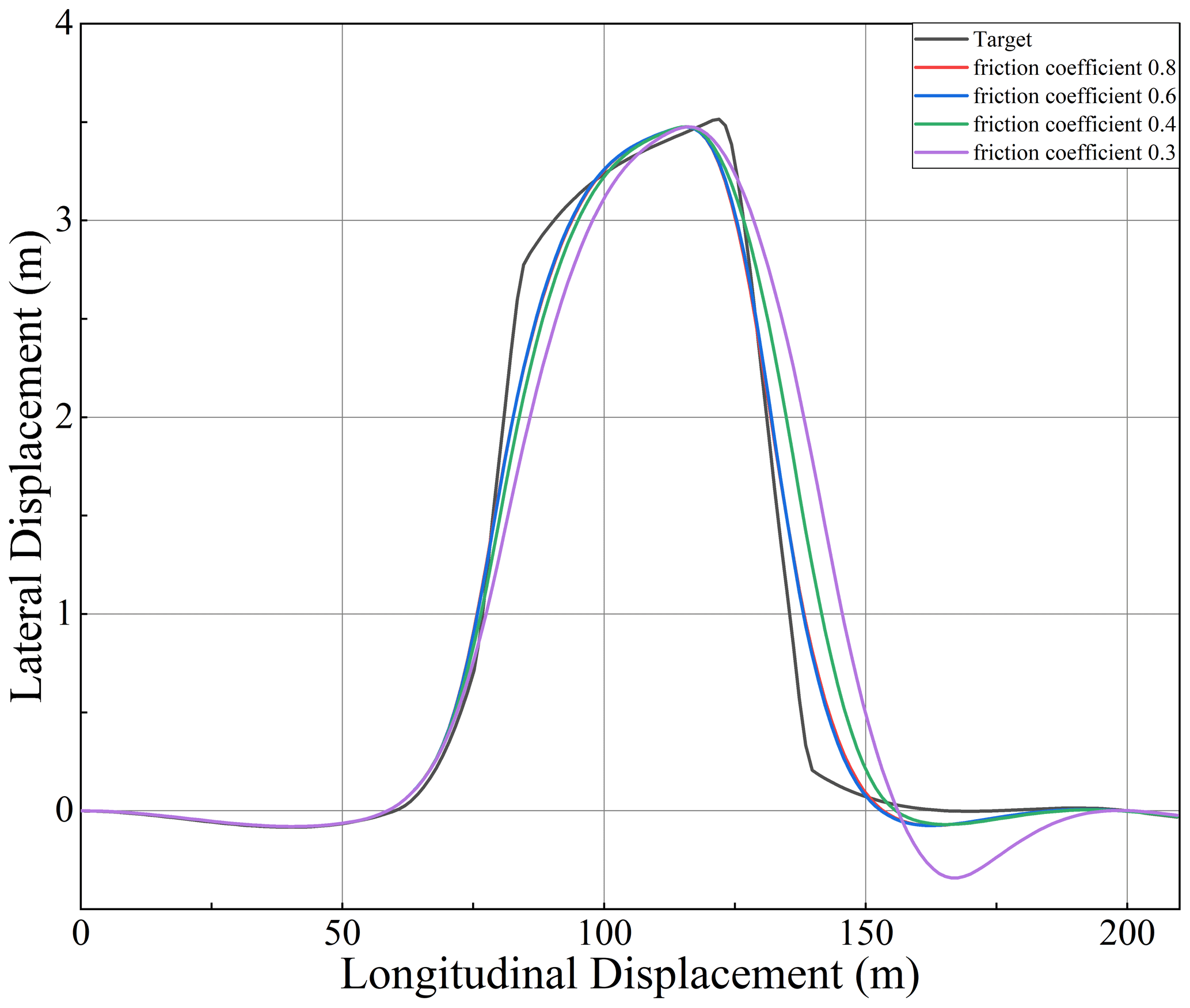
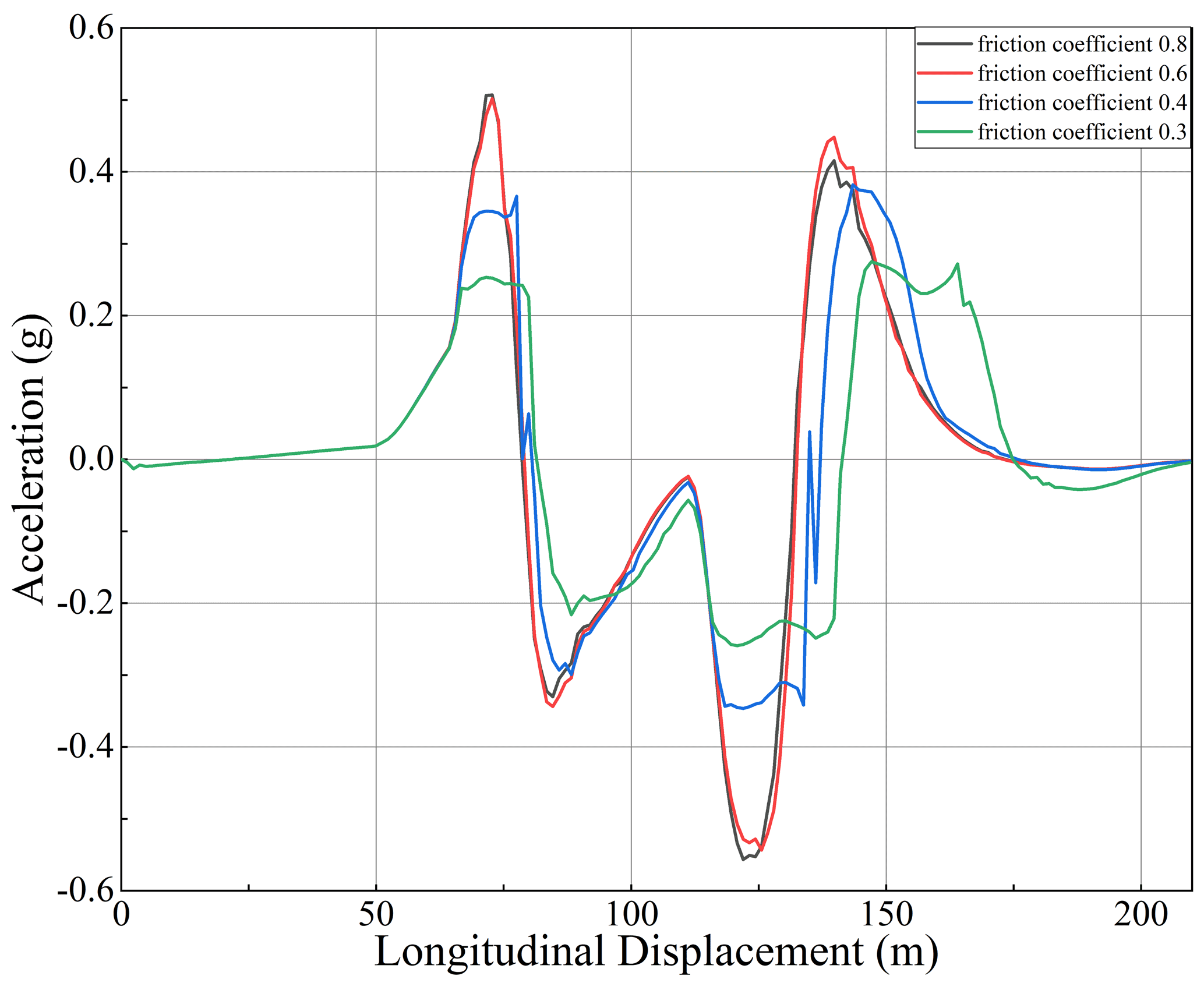
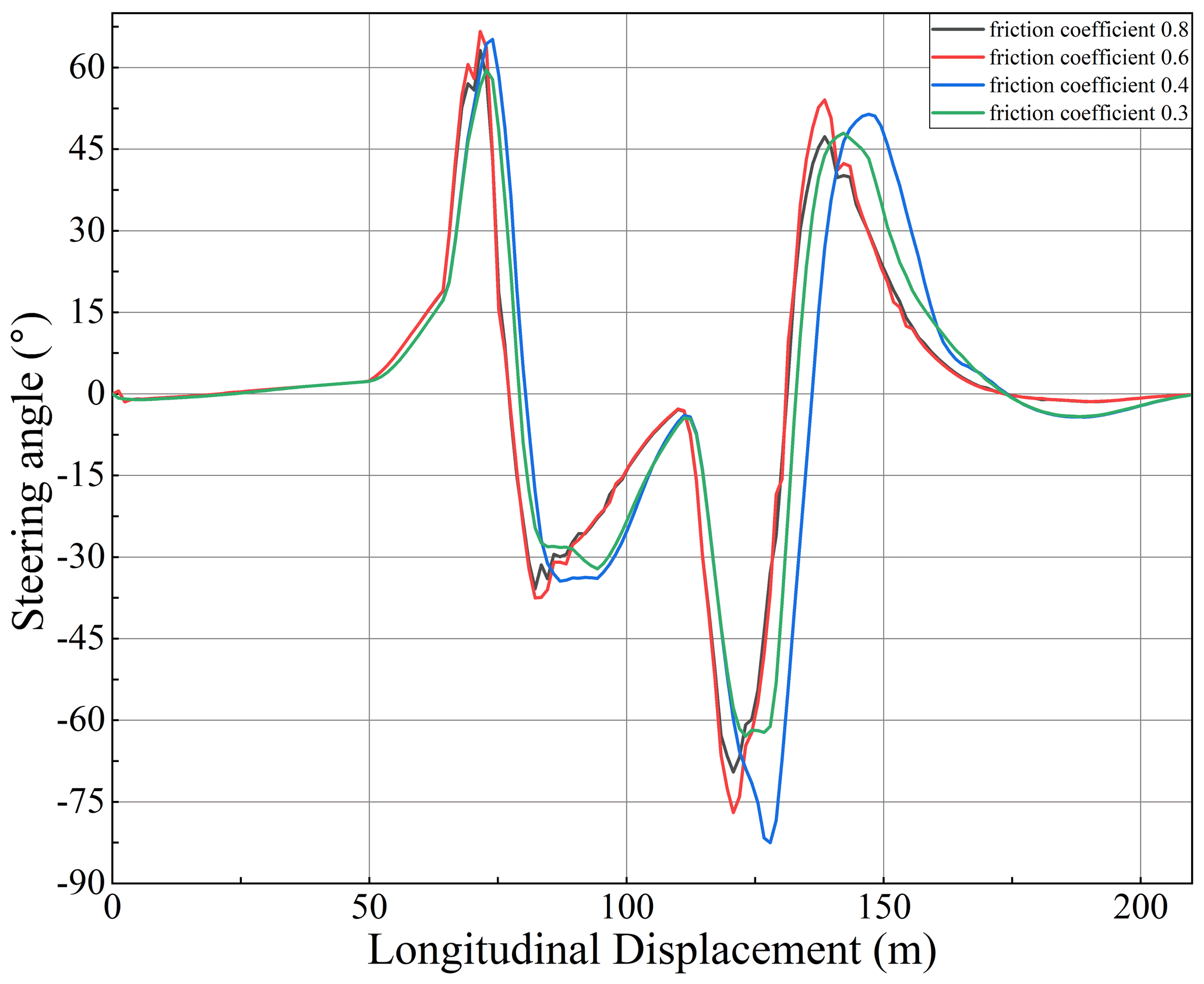
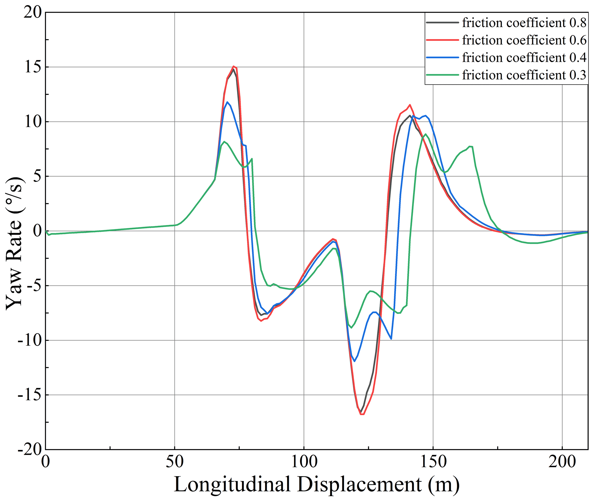
As shown in Figs. 13–16, the controller's accuracy decreases with the decrease in the road friction coefficient. After turning back to the front, the vehicle has a specific deviation, but it can also keep on the prescribed track. According to the variation law of lateral acceleration and yaw rate, the lateral acceleration and yaw rate decrease and have certain fluctuations when the road friction coefficient decreases. This may be due to the tires not providing enough lateral force. Although the control effect is slightly chattering, the chattering amplitude is small, and the lateral deviation does not increase significantly. Therefore, the designed controller can effectively track and control the vehicle lateral when a low road friction coefficient is present.
In order to verify the difference in the control effect between the designed fuzzy RBF neural network terminal sliding mode controller and other controllers, this paper compares the control effect between traditional PID controller, the terminal sliding mode controller(T-SMC), and fuzzy RBF neural network terminal sliding mode controller(T-Fuzzy-RBF-SMC). The speed is set to 15 m s−1, and the road friction coefficient is 0.8. The simulation results are shown in Figs. 17–20.
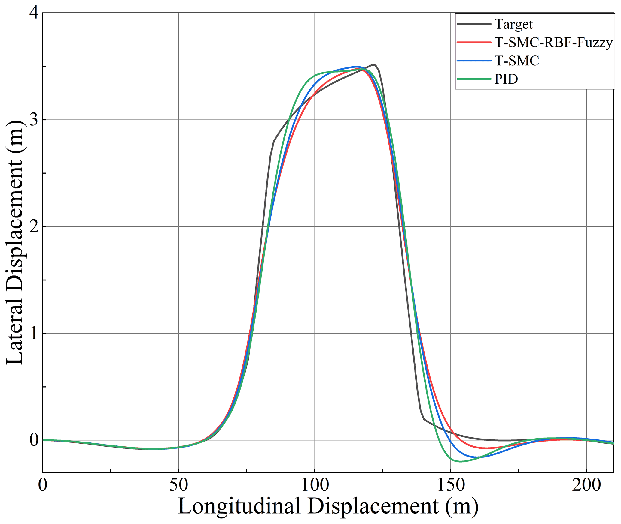
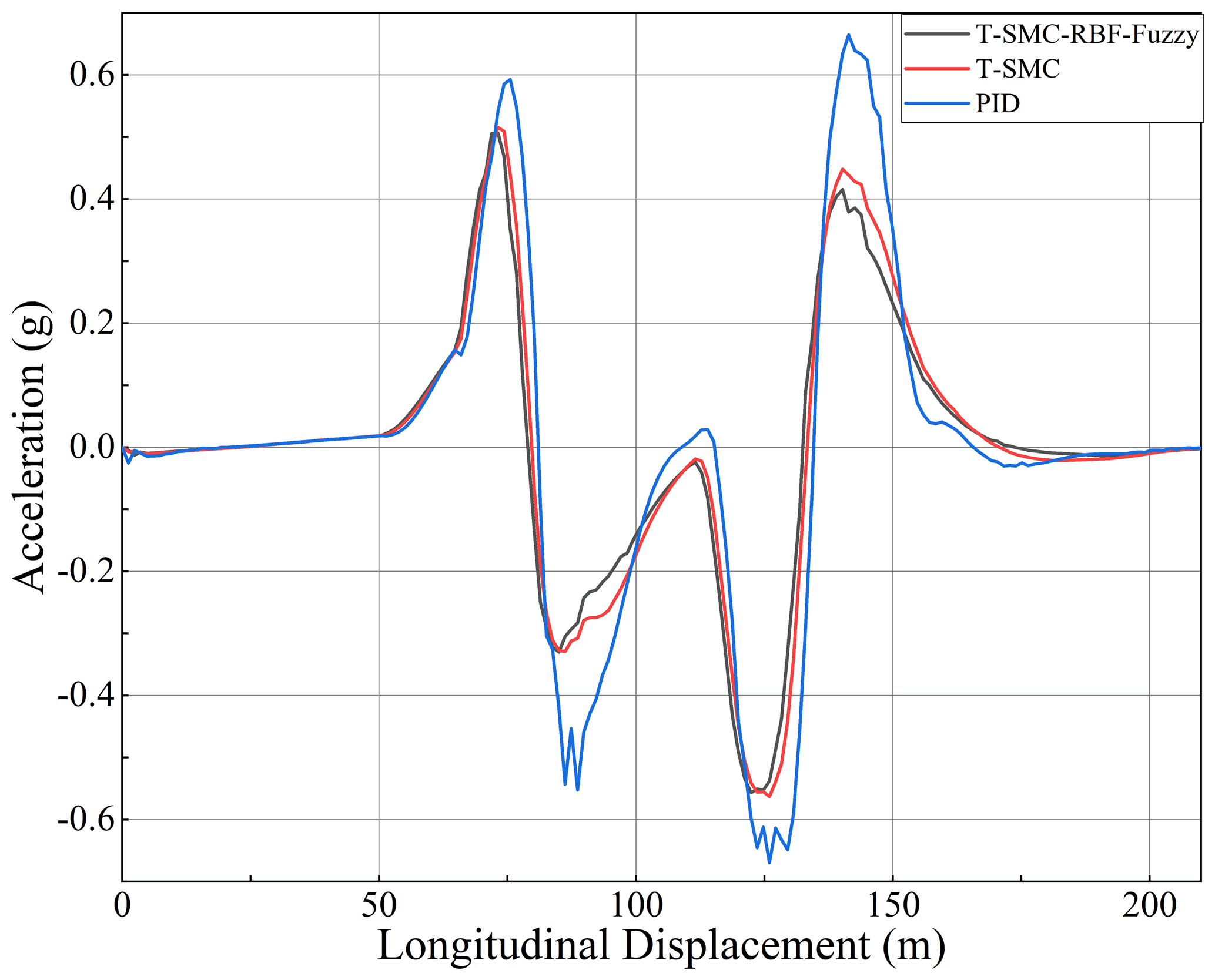
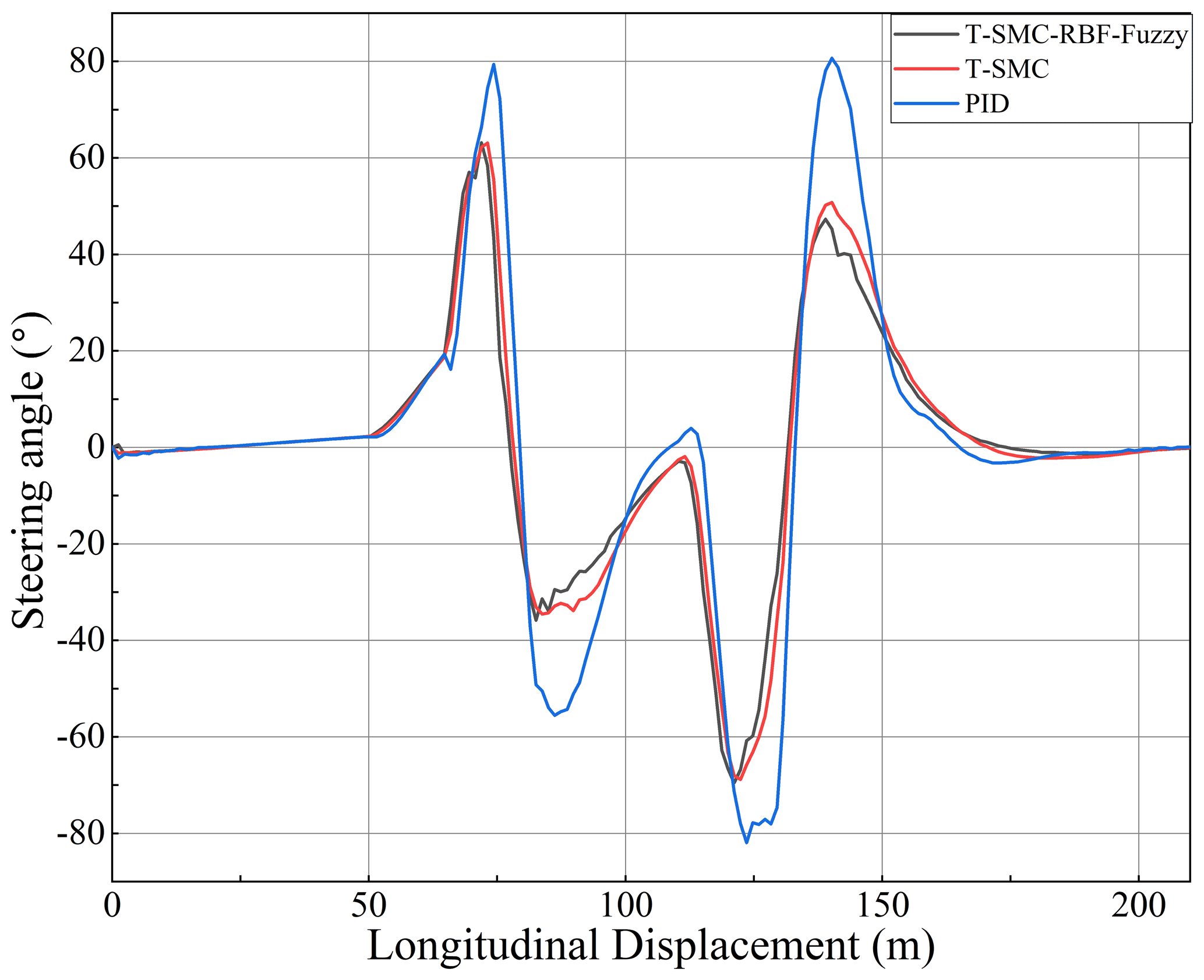

Figures 17–20 show that the three control methods effectively carry out vehicle trajectory tracking and lateral control. The controller designed in this paper has a better control effect than the traditional PID in trajectory tracking. It shows that the controller designed in this paper has a specific optimization in the control effect. Compared with the controller designed in this paper, the control effect of T-Fuzzy-RBF-SMC is better than that of T-SMC. The control variables of acceleration, steering wheel angle, and yaw rate are optimized, as compared with the T-SMC algorithm. Therefore, the fuzzy RBF neural network terminal sliding mode controller designed in this paper has a better control effect than the other two controllers.
This paper proposes a fuzzy RBF neural network terminal sliding mode controller for trajectory tracking control and lateral control of electric vehicles. A terminal sliding mode controller is used to design the controller, and the RBF neural network method is used to adaptive approximation of system parameters. In order to eliminate chattering, a fuzzy algorithm is designed for fuzzy control of control gain. The designed controller is verified by simulation. The simulation of different speeds, different road friction coefficients, and different controllers verified that the controller designed in this paper could effectively carry out trajectory tracking and lateral control of electric vehicles and eliminate chattering to a certain extent. In future research, we hope to improve the control algorithm and consider more uncertain parameters such as road conditions, changes in the centroid position caused by changes in vehicle quality, etc. At the same time, we also need to verify the algorithm designed in this paper on the test bench and the actual vehicle to ensure its timeliness.
The code and data included in this article can be made available by the corresponding author upon reasonable request. With respect to future applications, please note that the data and codes are confidential and cannot be made publicly available.
BW, YL, YF and XG designed research, performed research, analyzed data, and wrote the paper.
The contact author has declared that none of the authors has any competing interests.
Publisher's note: Copernicus Publications remains neutral with regard to jurisdictional claims in published maps and institutional affiliations.
The authors would like to thank the 13th Five-Year Science and Technology Project of Education Department of Jilin Province (grant no. JJKH20200957KJ) and Regional Innovation Co-operation Project of Department of Science and Technology of Sichuan Province (grant no. 2021YFQ0052).
This research has been funded by the 13th Five-Year Science and Technology Project of Education Department of Jilin Province (grant no. JJKH20200957KJ) and Regional Innovation Co-operation Project of Department of Science and Technology of Sichuan Province (grant no. 2021YFQ0052).
This paper was edited by Peng Yan and reviewed by two anonymous referees.
Abatari, H. T. and Tafti, A. D.: Using a fuzzy PID controller for the path following of a car-like mobile robot, First Rsi/ism International Conference on Robotics & Mechatronics, IEEE, https://doi.org/10.1109/ICRoM.2013.6510103, 2013.
Boumediene, S., Samira, C., and Hassane, A.: Fuzzy swarm trajectory tracking control of unmanned aerial vehicle, Journal of Computational Design and Engineering, 7, 435–447, https://doi.org/10.1093/jcde/qwaa036, 2020.
Cao, H., Song, X., Zhao, S., Bao, S., and Huang, Z.: An optimal model-based trajectory following architecture synthesising the lateral adaptive preview strategy and longitudinal velocity planning for highly automated vehicle, Vehicle Syst. Dyn., 55, 1143–1188, https://doi.org/10.1080/00423114.2017.1305114, 2017.
Chen, W., Tan, D., Wang, H., Wang, J., and Xia, G.: A Class of Driver Directional Control Model Based on Trajectory Prediction, Journal of Mechanical Engineering, 52, 106–115 https://doi.org/10.3901/JME.2016.14.106, 2016.
Dugoff, H., Fancher P. S., and Segel L.: An analysis of tire action properties and their influence on vehicle dynamic performance, SAE Transcations, 79, 1219–1243 https://doi.org/10.4271/700377, 1970.
Feng, T., Wang, Y., and Li, Q.: Coordinated control of active front steering and active disturbance rejection sliding mode-based DYC for 4WID-EV, Meas. Control, 53, 1870–1882, https://doi.org/10.1177/0020294020959111, 2020.
Gonzalo, D., Paul, R., and Choo, K.: Driverless vehicle security: Challenges and future research opportunities, Future Gener. Comp. Sy., 108, 1092–1111, https://doi.org/10.1016/j.future.2017.12.041, 2020.
Guo, J., Luo, Y., and Li, K.: An Adaptive Hierarchical Trajectory Following Control Approach of Autonomous Four-Wheel Independent Drive Electric Vehicles[J], IEEE T. Intell. Transp., 19, 2482–2492 https://doi.org/10.1109/TITS.2017.2749416, 2017.
Li, S. E., Chen, H., Li, R., Liu, Z., Wang, Z., and Xin Z.: Predictive lateral control to stabilise highly automated vehicles at tire-road friction limits, Vehicle Syst. Dyn., 58, 768–786, https://doi.org/10.1080/00423114.2020.1717553, 2020.
Liang, H., Li, G., Rong, T., and Deng L.: Unmanned vehicle trajectory tracking based on model predictive control, Automobile Applied Technology, 20, 53–55, https://doi.org/10.16638/j.cnki.1671-7988.2017.20.018, 2017.
Macadam, C. C.: Understanding and modeling the human driver[J], Vehicle Syst. Dyn., 40, 101–134 https://doi.org/10.1076/vesd.40.1.101.15875, 2003.
Martin, T. C., Orchard, M. E., and Sánchez, P. V.: Design and Simulation of Control Strategies for Trajectory Tracking in an Autonomous Ground Vehicle, 6th IFAC Conference on Management and Control of Production and Logistics, 46, 118–123, https://doi.org/10.3182/20130911-3-BR-3021.00096, 2013.
Norouzi, A., Masoumi, M., Barari, A., and Sani, S. F.: Lateral control of an autonomous vehicle using integrated back-stepping and sliding mode controller, P. I. Mech. Eng., 233, 141–151, https://doi.org/10.1177/1464419318797051, 2019.
Sun, Z., Zheng, J., Man, Z., and Fu, M.: Nested adaptive super-twisting sliding mode control design for a vehicle steer-by-wire system, Mech. Syst. Signal Pr., 122, 658–672, https://doi.org/10.1016/j.ymssp.2018.12.050, 2019.
Taghavifar, H. and Rakheja, S.: Path-tracking of autonomous vehicles using a novel adaptive robust exponential-like-sliding-mode fuzzy type-2 neural network controller, Mech. Syst. Signal Pr., 130, 41–55, https://doi.org/10.1016/j.ymssp.2019.04.060, 2019.
Tagne, G., Talj, R., and Charara, A.: Immersion and Invariance vs Sliding Mode Control for Reference Trajectory Tracking of Autonomous Vehicles, Control Conference, IEEE, https://doi.org/10.1109/ECC.2014.6862436, 2014.
Wang, X., Guo, L., and Jia, Y.: Road Condition Based Adaptive Model Predictive Control for Autonomous Vehicles, ASME 2018 Dynamic Systems and Control Conference, https://doi.org/10.1115/DSCC2018-9095, 2018.
Wu, Y., Wang, L., Zhang, J., and Li, F.: Path Following Control of Autonomous Ground Vehicle Based on Nonsingular Terminal Sliding Mode and Active Disturbance Rejection Control, IEEE T. Veh. Technol., 68, 6379–6390, https://doi.org/10.1109/TVT.2019.2916982, 2019.
Xiong, L., Yang, X., Zhuo, G., Leng, B., and Zhang, R.: Review on Motion Control of Autonomous Vehicles, Journal of Mechanical Engineering, 6, 127–143, https://doi.org/10.3901/JME.2020.10.127, 2020.
Yuan, S. T., Zhao, P. C , Zhang, Q. Y., and Hu, X.: Research on Model Predictive Control-based Trajectory Tracking for Unmanned Vehicles, 2019 4th International Conference on Control and Robotics Engineering (ICCRE), https://doi.org/10.1109/ICCRE.2019.8724158, 2019.
Zhang, C., Hu, J., Qiu, J., Yang, W., Sun, H., and Chen, Q.: A Novel Fuzzy Observer-Based Steering Control Approach for Path Tracking in Autonomous Vehicles, IEEE T. Fuzzy Syst., 27, 278–290, https://doi.org/10.1109/TFUZZ.2018.2856187, 2019.
Zhou, L., Wang, G., Sun, K., and Li, X.: Trajectory Tracking Study of Track Vehicles Based on Model Predictive Control, Journal of Mechanical Engineering, 65, 329–342, https://doi.org/10.5545/sv-jme.2019.5980, 2019.