Evolutionary multi-objective trajectory optimization for a redundant robot in Cartesian space considering obstacle avoidance

A method of end-effector trajectory planning in Cartesian space based on multi-objective optimization is proposed in this paper to solve the collision problem during the motion of the redundant manipulator. First, a cosine polynomial function is used to interpolate the trajectory of the end effector, enabling it to reach the desired pose at a specific time. Then, the joint trajectory of the manipulator is solved by inverse kinematics, and the null space term is introduced as the joint limit constraint in the inverse kinematics equation. During the operation of the manipulator, the collision detection algorithm is employed to calculate the distance between the obstacle and each arm in real time. Finally, a multi-objective, multi-optimization model of trajectory that considers the obstacle avoidance, joint velocity, joint jerk and energy consumption is established and optimized with a multi-objective particle swarm optimization algorithm. The simulation results demonstrate that the proposed method can effectively accomplish the trajectory planning task and avoid obstacles; the joint trajectories obtained are smooth and meet the limit constraints; the joint jerk and energy consumption are well suppressed.

1 Introduction

In many of today's vastly complex and difficult manufacturing applications, manipulators may have more degrees of freedom (DOFs) than essential due to the need of executing intended complicated jobs like human arms. Specifically, the end effector of redundant manipulator should satisfy a desired trajectory while its body avoids colliding with obstacles in the environment, contributing to finishing the job. The extremely crucial obstacle avoidance problem is that robotic manipulators are required to move from an initial pose to a specified final objective without colliding with any obstacles in the workspace.

To solve the trajectory planning problem considering obstacle avoidance, many researchers have focused on different methods. For example, Ma and Liang (2020) proposed an obstacle avoidance algorithm for a 6-DOF manipulator based on a sixth-degree polynomial, with limitations to the redundant manipulator. For the obstacle-avoiding motion of the end effector of the redundant robot, Shen et al. (2014) presented an obstacle avoidance algorithm based on the transition between the primary and the secondary tasks to acquire a smooth and continuous trajectory. Dalla and Pathak (2017) put forward a methodology that a limited number of joints are actuated and a curve-constrained link trajectory tracking is developed to control hyper-redundant space robots. However, these are only for planar robots. Shi et al. (2019) constructed a visual servoing system, which obtained the image errors by the ORB feature points and constructed a virtual repulsion torque to avoid obstacles.

In addition to the above methods, more researchers handle the obstacle avoidance problem by introducing the concept of potential field to construct the artificial potential field. Safeea et al. (2020) redefined the obstacle avoidance problem as a second-order optimization problem and constructed the potential function that is minimized by Newton's method to realize real-time trajectory calculation in joint space. It lacks the intuitiveness and efficiency compared with Cartesian space trajectory planning. Wang et al. (2018) realized trajectory planning and obstacle avoidance through the improved artificial potential field method with the consideration of both position and posture of manipulator end effectors. Park et al. (2020) employed a Jacobian matrix-based numerical method and an improved potential field method to achieve path planning and obstacle avoidance, both in redundant and non-redundant conditions.

The above-mentioned trajectory planning methods focus more on obstacle avoidance than kinematics or dynamics optimization. Nowadays, an optimized path should be found for robot motion regarding minimum time (Bourbonnais et al., 2015), minimum distance (Salaris et al., 2010), and minimum energy (Arakelian et al., 2011) given the robot optimization problem in obstacle avoidance planning. This suggests that multiple objective functions should be simultaneously optimized to obtain a suitable trajectory. Based on the above articles, some criteria for evaluating manipulator trajectory can be obtained:

1. Trajectories need to be predictable, accurate, and effective to both compute and execute.

2. Trajectories need to ensure that the joints of the robotic arm do not appear singular.

3. Trajectories should be found for a manipulator with respect to minimum time, minimum distance, and minimum energy.

Many researchers used an evolutionary algorithm to address multi-objective planning problems considering obstacle avoidance. For example, Saravanan et al. (2008) optimized two evolutionary algorithms of an elite non-dominant sorting genetic algorithm (NSGA-II) and differential evolution (DE) to handle the multi-objective problem and achieved the predetermined goal in the PUMA560 robot. Han et al. (2013) realized the obstacle avoidance path planning optimization of the robot arm in the environment with single or multiple obstacles based on genetic algorithms with execution time, space distance, and trajectory length as the optimization parameters. However, most of the above researchers have weighted each constraint as an objective function, making the result very dependent on the setting of the weight factor. Some researchers transform multi-objective problems into quadratic programming (QP) problems. Chen and Zhang (2017) proposed a hybrid multi-objective scheme including the specified primary task for the end effector, obstacle avoidance, joint-physical limits avoidance, and repetitive motion of redundant robot manipulators and transformed it into a dynamic quadratic program (DQP) problem. Zhang et al. (2020) studied two schemes of hybrid end-effector pose-maintaining and obstacle-limits avoidance (PM-OLA) for redundant robot motion planning based on QP framework to solve the end-effector drift problem in the planar task. Other researchers obtained the Pareto front in multi-objective problems, as well as the non-dominant solution. Guigue et al. (2010) employed the discrete dynamic programming (DDP) approximation method to obtain an approximate solution of the Pareto optimal set to handle multi-objective robotic trajectory planning problems. Marcos et al. (2012) combined a closed-loop pseudo-inverse method with a multi-objective genetic algorithm to control the joint position and choose a solution from the Pareto solution set. Although these researchers solved the multi-objective problem, they did not add energy consumption constraint to the multi-objective problem for obtaining a superior solution with more energy-saving or less joint jerk.

Besides, many researchers have improved the particle swarm optimization (PSO) algorithm to acquire the optimized trajectory of the robotic arm. Cao et al. (2016) adopted a hybrid algorithm combing crossover and mutation particle swarm optimization (CMPSO) with the interior point method (IPM) to determine the minimum-length motion path of robot end effector and the best movement posture of the robot arm. Lin (2014) proposed a k-means clustering method based on PSO to address the near-optimal solution of the minimum-jerk joint trajectory, making it easy to obtain the optimized trajectory control law. Kucuk (2017) developed an optimal trajectory generation algorithm (OTGA) for generating smooth motion trajectories with minimum time with the PSO algorithm. Under the diversification of robot optimization goals, some researchers used a multi-objective particle swarm optimization (MOPSO) algorithm (Coello Coello and Lechuga, 2002) to solve multi-objective optimization problems. For instance, Yan et al. (2020) presented multi-objective configuration optimization for the maximum maneuverability and minimum base disturbance in the pre-contact stage of dual-arm space robot by MOPSO. Liu and Zhang (2021) proposed an improved external archives self-searching multi-objective particle swarm optimization (EASS-MOPSO) algorithm to handle the multi-objective trajectory optimization problem.

In this paper, regarding obstacle avoidance, the change rate of joint torque, joint angular velocity, and energy consumption are minimized using the path planning method based on a multi-objective optimization algorithm. The main contributions of this paper are highlighted as follows.

1. A cosine polynomial function is used to interpolate the trajectory of the end effector, enabling it to reach the desired pose at a specific time, and the null space term is introduced as the joint limit constraint in the inverse kinematics equation.

2. During the operation of the manipulator, a collision detection algorithm is employed to calculate the distance between the obstacle and each arm in real time.

3. The trajectory optimization model of redundant manipulator was established to consider obstacle avoidance, joint velocity, joint jerk and energy consumption, and the optimized trajectories were obtained by a multi-objective particle swarm optimization algorithm.

The remaining paper is organized as follows. In Sect. 2, the end trajectory of the robotic arm is interpolated using the cosine fifth-degree polynomial, allowing the end to reach the specified pose at the specified time. Then, the joint trajectory of the robotic arm is reversed through inverse kinematics. Section 3 presents the collision detection algorithm used in this paper. Afterward, the multi-objective optimization problem equations are described in Sect. 4. The obstacle avoidance trajectory planning based on multi-objective optimization is introduced in Sect. 5. Simulation results are analyzed in Sect. 6. Finally, conclusions are drawn in Sect. 7.

2 Trajectory planning of redundant manipulator

2.1 Trajectory parameterization of end effector in Cartesian space

A five-order cosine polynomial is adopted to describe the trajectory to ensure the position, orientation, velocity, and acceleration of the end effector change smoothly and continuously. With this method, the motion of the end effector follows a helical curve in Cartesian space (Zghal et al., 1990). The pose of the end effector is taken to compose a six-dimensional generalized coordinate vector ${\mathit{X}}_{\mathrm{e}}={\left[X_{\mathrm{1}}\left(t\right),\mathrm{\dots },X_{\mathrm{6}}\left(t\right)\right]}^{\mathrm{T}}$ as the status variable of the system. The trajectory is parameterized as

$$\begin{array}{}\text{(1)}& \begin{array}{rl}{X}_j\left(t\right)& =\left({\mathit{\lambda }}_{j\mathrm{5}}{t}^{\mathrm{5}}+{\mathit{\lambda }}_{j\mathrm{4}}{t}^{\mathrm{4}}+{\mathit{\lambda }}_{j\mathrm{3}}{t}^{\mathrm{3}}+{\mathit{\lambda }}_{j\mathrm{2}}{t}^{\mathrm{2}}+{\mathit{\lambda }}_{j\mathrm{1}}t+{\mathit{\lambda }}_{j\mathrm{0}}\right)\\ & \cdot \cos \left({\displaystyle \frac{\mathrm{2}\mathit{\pi }t}{T_j}}+{\mathit{\phi }}_j\right)+X_{j\mathrm{0}},\end{array}\end{array}$$

where X_j0 denotes the initial pose of end effector, and λ, T and φ are trajectory parameters, $j=\mathrm{1},\mathrm{\dots },\mathrm{6}$.

By taking the differential of the equation above, the generalized velocity and acceleration of the end effector can be expressed as

$$\begin{array}{}\text{(2)}& \begin{array}{ll}{\dot{X}}_j\left(t\right)& =K_{j\mathrm{1}}\left(t\right)\cos \left(\frac{\mathrm{2}\mathit{\pi }t}{T_j}+{\mathit{\phi }}_j\right)\\ & -\frac{\mathrm{2}\mathit{\pi }}{T_j}{K}_{j\mathrm{2}}\left(t\right)\sin \left(\frac{\mathrm{2}\mathit{\pi }t}{T_j}+{\mathit{\phi }}_j\right)\\ {\ddot{X}}_j\left(t\right)& =K_{j\mathrm{3}}\left(t\right)\cos \left(\frac{\mathrm{2}\mathit{\pi }t}{T_j}+{\mathit{\phi }}_j\right)\\ & -\frac{\mathrm{4}\mathit{\pi }}{T_j}{K}_{j\mathrm{1}}\left(t\right)\sin \left(\frac{\mathrm{2}\mathit{\pi }t}{T_j}+{\mathit{\phi }}_j\right)\\ & -\frac{\mathrm{4}{\mathit{\pi }}^{\mathrm{2}}}{T_j^{\mathrm{2}}}{K}_{j\mathrm{2}}\left(t\right)\cos \left(\frac{\mathrm{2}\mathit{\pi }t}{T_j}+{\mathit{\phi }}_j\right),\end{array}\end{array}$$

where K_j(t) can be described as follows:

$$\begin{array}{}\text{(3)}& \begin{array}{ll}{K}_{j\mathrm{1}}\left(t\right)& =\mathrm{5}{\mathit{\lambda }}_{j\mathrm{5}}{t}^{\mathrm{4}}+\mathrm{4}{\mathit{\lambda }}_{j\mathrm{4}}{t}^{\mathrm{3}}+\mathrm{3}{\mathit{\lambda }}_{j\mathrm{3}}{t}^{\mathrm{2}}+\mathrm{2}{\mathit{\lambda }}_{j\mathrm{2}}t+{\mathit{\lambda }}_{j\mathrm{1}}\\ K_{j\mathrm{2}}\left(t\right)& ={\mathit{\lambda }}_{j\mathrm{5}}{t}^{\mathrm{5}}+{\mathit{\lambda }}_{j\mathrm{4}}{t}^{\mathrm{4}}+{\mathit{\lambda }}_{j\mathrm{3}}{t}^{\mathrm{3}}+{\mathit{\lambda }}_{j\mathrm{2}}{t}^{\mathrm{2}}+{\mathit{\lambda }}_{j\mathrm{1}}t+{\mathit{\lambda }}_{j\mathrm{0}}\\ K_{j\mathrm{3}}\left(t\right)& =\mathrm{20}{\mathit{\lambda }}_{j\mathrm{5}}{t}^{\mathrm{3}}+\mathrm{12}{\mathit{\lambda }}_{j\mathrm{4}}{t}^{\mathrm{2}}+\mathrm{6}{\mathit{\lambda }}_{j\mathrm{3}}t+\mathrm{2}{\mathit{\lambda }}_{j\mathrm{2}}.\end{array}\end{array}$$

The boundary conditions of the trajectory planning problem are

$$\begin{array}{}\text{(4)}& \begin{array}{ll}{X}_j\left(t_{\mathrm{0}}\right)& =X_{j\mathrm{0}},{\dot{X}}_j\left(t_{\mathrm{0}}\right)={\ddot{X}}_j\left(t_{\mathrm{0}}\right)=\mathrm{0}\\ X_j\left(t_{\mathrm{f}}\right)& =X_{j\mathrm{f}},{\dot{X}}_j\left(t_{\mathrm{f}}\right)=\mathrm{0},{\ddot{X}}_j\left(t_{\mathrm{f}}\right)=\mathrm{0},\end{array}\end{array}$$

where t₀ and t_f represent the initial and final time, respectively; X_jf refers to the desired pose of end effector.

By substituting Eq. (4) into Eqs. (1) and (2), the following relationship can be obtained:

$$\begin{array}{}\text{(5)}& \begin{array}{ll}{\mathit{\lambda }}_{j\mathrm{0}}& ={\mathit{\lambda }}_{j\mathrm{1}}={\mathit{\lambda }}_{j\mathrm{2}}=\mathrm{0}\\ {\mathit{\lambda }}_{j\mathrm{3}}& =\frac{\begin{array}{c}\mathrm{2}\left(\mathrm{2}{\mathit{\pi }}^{\mathrm{2}}{D}_j{t}_{\mathrm{f}}^{\mathrm{2}}{\sin }^{\mathrm{2}}\right(\mathit{\psi })+{\mathit{\pi }}^{\mathrm{2}}{D}_j{t}_{\mathrm{f}}^{\mathrm{2}}{\cos }^{\mathrm{2}}(\mathit{\psi })\\ -\mathrm{4}\mathit{\pi }{D}_j{T}_j{t}_{\mathrm{f}}\sin \left(\mathit{\psi }\right)\cos \left(\mathit{\psi }\right)+\mathrm{5}{D}_j{T}_j^{\mathrm{2}}{\cos }^{\mathrm{2}}\left(\mathit{\psi }\right))\end{array}}{T_j^{\mathrm{2}}{t}_{\mathrm{f}}^{\mathrm{3}}{\cos }^{\mathrm{3}}\left(\mathit{\psi }\right)}\\ {\mathit{\lambda }}_{j\mathrm{4}}& =\frac{\begin{array}{c}-\left[D_j\right(\mathrm{8}{\mathit{\pi }}^{\mathrm{2}}{t}_{\mathrm{f}}^{\mathrm{2}}{\sin }^{\mathrm{2}}\left(\mathit{\psi }\right)+\mathrm{4}{\mathit{\pi }}^{\mathrm{2}}{t}_{\mathrm{f}}^{\mathrm{2}}{\cos }^{\mathrm{2}}\left(\mathit{\psi }\right)\\ -\mathrm{14}\mathit{\pi }{T}_j{t}_{\mathrm{f}}\sin \left(\mathit{\psi }\right)\cos \left(\mathit{\psi }\right)+\mathrm{15}{T}_j^{\mathrm{2}}{\cos }^{\mathrm{2}}\left(\mathit{\psi }\right)\left)\right]\end{array}}{T_j^{\mathrm{2}}{t}_{\mathrm{f}}^{\mathrm{4}}{\cos }^{\mathrm{3}}\left(\mathit{\psi }\right)}\\ {\mathit{\lambda }}_{j\mathrm{5}}& =\frac{\begin{array}{c}\mathrm{2}{D}_j\left(\mathrm{2}{\mathit{\pi }}^{\mathrm{2}}{t}_{\mathrm{f}}^{\mathrm{2}}{\sin }^{\mathrm{2}}\right(\mathit{\psi })+{\mathit{\pi }}^{\mathrm{2}}{t}_{\mathrm{f}}^{\mathrm{2}}{\cos }^{\mathrm{2}}(\mathit{\psi })\\ -\mathrm{3}\mathit{\pi }{T}_j{t}_{\mathrm{f}}\sin \left(\mathit{\psi }\right)\cos \left(\mathit{\psi }\right)+\mathrm{3}{T}_j^{\mathrm{2}}{\cos }^{\mathrm{2}}\left(\mathit{\psi }\right))\end{array}}{T_j^{\mathrm{2}}{t}_{\mathrm{f}}^{\mathrm{5}}{\cos }^{\mathrm{3}}\left(\mathit{\psi }\right)},\end{array}\end{array}$$

where ψ and D_j can be described as

$$\begin{array}{}\text{(6)}& \begin{array}{ll}\mathit{\psi }& =\frac{\mathrm{2}\mathit{\pi }{t}_{\mathrm{f}}}{T_j}+{\mathit{\phi }}_j\\ D_j& =X_{j\mathrm{f}}-X_{j\mathrm{0}}.\end{array}\end{array}$$

According to Eq. (5), polynomial coefficients can be determined with parameters T_j and φ_j.

Then trajectories of end effector that satisfy the constraints can be obtained with the following parameters vector:

$$\begin{array}{}\text{(7)}& \mathit{\xi }={\left[T_{\mathrm{1}},{\mathit{\phi }}_{\mathrm{1}},T_{\mathrm{2}},{\mathit{\phi }}_{\mathrm{2}},\mathrm{\dots },T_{\mathrm{6}},{\mathit{\phi }}_{\mathrm{6}}\right]}^{\mathrm{T}}.\end{array}$$

2.2 Joint motion planning for redundant manipulator

The subject of this paper is a n-DOF redundant manipulator. Assuming the dimension of task space is m(m≤6), a redundant manipulator satisfies n>m. The joint velocity vector of redundant manipulator is

$$\begin{array}{}\text{(8)}& \dot{\mathit{q}}={\mathbf{J}}^{+}{\dot{\mathit{x}}}_e+\left(\mathbf{I}-{\mathbf{J}}^{+}\mathbf{J}\right)\dot{\mathbf{\Phi }},\end{array}$$

where x_e∈ℝ^m indicates the pose of end effector in Cartesian space; q∈ℝⁿ denotes joint angle vector; $\mathbf{J}\in {\mathbb{R}}^{n\times m}$ represents the Jacobian matrix of manipulator; $\mathbf{I}\in {\mathbb{R}}^{n\times n}$ refer to unit matrix; $\dot{\mathbf{\Phi }}\in {\mathbb{R}}^n$ stands for an arbitrary n-dimensional vector; $(\mathbf{I}-{\mathbf{J}}^{+}\mathbf{J})\in {\mathbb{R}}^{n\times n}$ designates the null space projection matrix; ${\mathbf{J}}^{+}\in {\mathbb{R}}^{n\times m}$ means the generalized inverse of the Jacobian matrix, which is defined by

$$\begin{array}{}\text{(9)}& {\mathbf{J}}^{+}={\mathbf{J}}^{\mathrm{T}}{\left({\mathbf{JJ}}^{\mathrm{T}}\right)}^{-\mathrm{1}}.\end{array}$$

For redundant manipulators, a specific trajectory of end effector can be obtained by multiple joint trajectories. Hence, the joint trajectory should be selected to ensure that the motion of the manipulator follows specific constraints. Null space (Zghal et al., 1990) term is introduced in this paper to enable the joint motion to satisfy joint limit constraints. The joint limit constraint function is established as

$$\begin{array}{}\text{(10)}& H\left(q\right)={\sum }_{i=\mathrm{1}}^n{\displaystyle \frac{\left(q_{i\max }-q_{i\min }\right)}{\left(q_{i\max }-q_i\right)\left(q_i-q_{i\min }\right)}},\end{array}$$

where q_i donates the angle of joint i; q_imax and q_imin represent upper and lower limits of joint i, respectively.

According to the gradient projection method, the joint angle limit constraints are resolved by substituting k∇H(q) for $\dot{\mathbf{\Phi }}$ in Eq. (8) as

$$\begin{array}{}\text{(11)}& \dot{\mathit{q}}={\mathbf{J}}^{+}{\dot{\mathit{x}}}_{\mathrm{e}}+k(\mathbf{I}-{\mathbf{J}}^{+}\mathbf{J})\mathrm{\nabla }\mathit{H}\left(\mathit{q}\right),\end{array}$$

where the gradient vector ∇H(q) is given by

$$\begin{array}{}\text{(12)}& \mathrm{\nabla }\mathit{H}\left(\mathit{q}\right)=\left({\displaystyle \frac{\partial \mathit{H}\left(\mathit{q}\right)}{\partial q_{\mathrm{1}}}},{\displaystyle \frac{\partial \mathit{H}\left(\mathit{q}\right)}{\partial q_{\mathrm{2}}}},\mathrm{\dots },{\displaystyle \frac{\partial \mathit{H}\left(\mathit{q}\right)}{\partial q_n}}\right).\end{array}$$

∇H(q) reaches minimum value when $q_i=(q_{i\min }+q_{i\max })/\mathrm{2}$; ∇H(q) approaches to infinity when q_i=q_imin or q_i=q_imax.

3 Collision detection algorithm

A collision detection algorithm should be established to achieve obstacle avoidance. A redundant manipulator is explored in this paper. Most of the links are like cuboids or cylinders. Moreover, obstacles are irregular geometric objects. The collision detection between the manipulator and obstacles is extremely complicated. Thus, sphere and cylindrical envelopes are applied in this paper to describe the manipulator links, joints, and obstacles.

3.1 The description of space geometry relation

Considering that obstacles in three-dimensional space generally have irregular geometric shapes and various kinds, it is difficult to extract their boundary contours. Thus, regular body envelopment is adopted in this paper to simplify the obstacle model, so as to simplify the complexity of obstacle modeling. For example, the cylindrical envelopment model and sphere envelopment model are employed for slender rod and rounded objects, respectively. This modeling method expands the range of obstacles while guaranteeing the reliability of the collision detection algorithm.

The obstacle uses a sphere envelope, as illustrated in Fig. 1. The radius of the sphere is r_S. The cylindrical envelope is used for the links of the manipulator while the sphere envelope and cylindrical envelope are adopted to describe the joint. In this paper, a 7-DOF redundant manipulator (Fig. 5) is studied. As exhibited in Fig. 2. The two typical cases are described as follows.

1. For case I, when axes of adjacent links are vertical, straight connecting links (link i−1 and link i) are enveloped by cylinders whose axes are coplanar. The intersection points P_i of cylindrical axes are centers of joint envelope spheres. The radius of the cylinder for the link i is r_i; the radius of the sphere for the joint i is $r_i^j\ge \sqrt{r_i^{\mathrm{2}}+r_{i-\mathrm{1}}^{\mathrm{2}}}$. Hence, the distance between links and obstacles can be substituted as the distance from a line segment to a point in 3-dimensional space.

2. For case II, when axes of adjacent links are parallel, joint i and link i−1 are enveloped in the same way as case I considering the joint with offset. Hence, $r_i^j\ge \sqrt{r_{\mathrm{joint}}^{\mathrm{2}}+r_{i-\mathrm{1}}^{\mathrm{2}}}$, where r_joint indicates the radius of envelope cylinder for joint i. Two cylinders whose axes are coplanar and a sphere whose center is located in the intersection point (P_i) of the axes are applied to envelop it.

Figure 1 The obstacle uses sphere envelope.

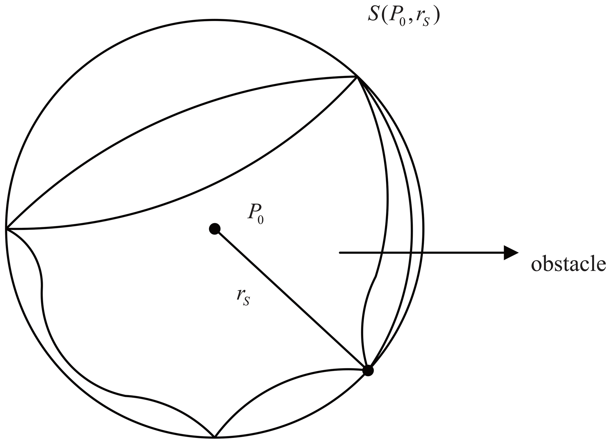
Figure 2 Links of the manipulator use cylindrical envelope and sphere envelope. (a) Case I. (b) Case II.

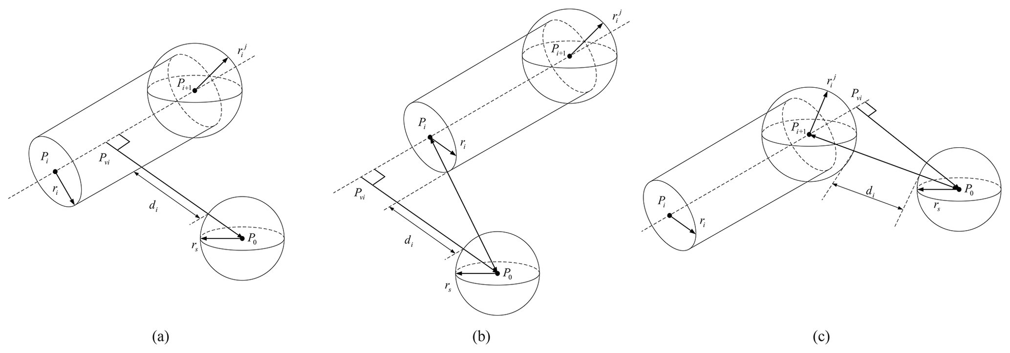
Figure 3 The space geometry relations between manipulator's links and obstacle. (a) Class I. (b) Class II. (c) Class III.

3.2 Collision detection algorithm

The space geometry (Guan et al., 2015) relations between manipulator's links and obstacle are divided into three classes, as exhibited in Fig. 3. Whether the links and obstacle collide depends on d_i, it denotes the minimum distance between the obstacle and manipulator's link/joint. If d_i>0, the obstacle is avoided; otherwise, it collides with the manipulator. Therefore, the collision detection problem between cylinder and sphere can be reduced to the calculation of the shortest distance between a point and line segment in 3D space.

Assume the length of link i is L_i. Centers of the bottom are P_i and P_i+1. A vertical line of segment P_iP_i+1 is drawn through P₀, and P_vi indicates the point of intersection to the cylindrical axis.

Based on the space geometry relation, the collision detection algorithm (Cheng et al., 1993) to achieve obstacle avoidance path planning for redundant manipulators is summarized as follows.

Step 1. Based on forwarding kinematics, the coordinates P_i of all nodes and joints are calculated with the current configuration and geometrical sizes of the manipulator.

The relative translation and rotation between link i coordinate and link i−1 coordinate can be described with a homogeneous transformation matrix $T_{i-\mathrm{1}}^i$. The kinematics equation of n degree of freedom manipulators can be expressed as

$$\begin{array}{}\text{(13)}& T_i^{\mathrm{0}}={\prod }_{j=\mathrm{1}}^i{T}_j^{j-\mathrm{1}}.\end{array}$$

Step 2. P_iP_vi is defined as the projection vector of P_iP₀ on P_iP_i+1, and the scale factor λ is calculated:

$$\begin{array}{}\text{(14)}& \mathit{\lambda }={\displaystyle \frac{{\mathit{P}}_i{\mathit{P}}_{vi}}{{\mathit{P}}_i{\mathit{P}}_{i+\mathrm{1}}}}={\displaystyle \frac{{\mathit{P}}_i{\mathit{P}}_{\mathrm{0}}\cdot {\mathit{P}}_i{\mathit{P}}_{i+\mathrm{1}}}{{\mathit{P}}_i{\mathit{P}}_{i+\mathrm{1}}\cdot {\mathit{P}}_i{\mathit{P}}_{i+\mathrm{1}}}}.\end{array}$$

The three-dimensional coordinates of the perpendicular foot P_vi can be obtained with $P_{vi}=P_i+\mathit{\lambda }(P_{i+\mathrm{1}}-P_i)$.

Step 3. The minimal distance from the links/joints to the obstacles is calculated. There are three possible positions of perpendicular foot P_vi related to P_iP_i+1:

• For class I, P_vi is on P_iP_i+1 when $\le \mathit{\lambda }\le \mathrm{1}$.

• For class II, P_vi is on the reverse extension of P_iP_i+1 when λ<0.

• For class III, P_vi is on the extension of P_iP_i+1 when λ>1.

Therefore, the minimum distance between P₀ and P_iP_i+1 is

$$\begin{array}{}\text{(15)}& d_i=\left\{\begin{array}{l}∥{\mathit{P}}_{\mathrm{0}}{\mathit{P}}_{vi}∥-r_i-r_{\mathrm{S}},\mathit{\lambda }<\mathrm{0}\\ min\mathit{\{}∥{\mathit{P}}_{\mathrm{0}}{\mathit{P}}_{i+\mathrm{1}}∥-r_i^j\\ -r_{\mathrm{S}},∥{\mathit{P}}_{\mathrm{0}}{\mathit{P}}_{vi}∥-r_i-r_{\mathrm{S}}\mathit{\}},\mathrm{0}\le \mathit{\lambda }\le \mathrm{1}\\ ∥{\mathit{P}}_{\mathrm{0}}{\mathit{P}}_{i+\mathrm{1}}∥-r_i^j-r_{\mathrm{S}},\mathit{\lambda }>\mathrm{1}\end{array}\right..\end{array}$$

Step 4. If $min\mathit{\{}{d}_{\mathrm{1}},d_{\mathrm{2}},\mathrm{\dots },d_n\mathit{\}}<\mathrm{0}$, a collision occurs. Then, the collision information is outputted. According to the collision condition, obstacles can be avoided if $min\mathit{\{}{d}_{\mathrm{1}},d_{\mathrm{2}},\mathrm{\dots },d_n\mathit{\}}>\mathrm{0}$.

Figure 4 The maintenance process of external repository.

4 Description of multi-objective trajectory planning problem

In this study, minimization of total energy, joint jerks, and avoidance of obstacles are considered together to build a multi-criterion cost function. Singularity involved in null space and joint limits is considered a constraint.

4.1 Establishment of objective functions

1. For a given trajectory of the end effector, the smaller the joint velocity is, the less likely the joint angle mutation occurs. Therefore, the optimization of joint angular velocity has the effect of avoiding singularity. Meanwhile, the null space term is used to constrain the joint limit when solving inverse kinematics. Since the collision detection algorithm is also the kinematic solution of the manipulator in essence, the obstacle avoidance term is taken as a penalty function in this paper to fuse with the joint angular velocity optimization objective. The specific expression is

   $$\begin{array}{}\text{(16)}& \mathrm{obt}=\left\{\begin{array}{l}{\mathit{\lambda }}_{\mathrm{1}}\cdot max\left\{-d_{\mathrm{1}},-d_{\mathrm{2}},\mathrm{\dots },-d_n\right\},\\ min\mathit{\{}{d}_{\mathrm{1}},d_{\mathrm{2}},\mathrm{\dots },d_n\mathit{\}}>\mathrm{0}\\ {\mathit{\lambda }}_{\mathrm{2}},min\mathit{\{}{d}_{\mathrm{1}},d_{\mathrm{2}},\mathrm{\dots },d_n\mathit{\}}<\mathrm{0}\end{array}\right.,\end{array}$$

   where obt denotes obstacle avoidance term; λ₁ and λ₂ are scale factors.

   Combining with Eq. (11), the kinematic optimization term can be expressed as

   $$\begin{array}{}\text{(17)}& f_{\mathrm{1}}=min{\sum }_{i=\mathrm{1}}^n\left(\left|{\dot{q}}_i\right|\right)+\mathrm{obt}.\end{array}$$

   Due to the scale factors, joint angular velocity is the major term when obstacles are avoided. Besides, the objective function is larger when the links failed to avoid the obstacle. This is convenient for choosing feasible solutions in the process of trajectory optimization.

2. For redundant manipulators, the frequent changes in the joint jerk would cause a great impact. Reducing the joint jerk can indirectly limit the change rate of joint torque and thus make the movement of the manipulator more stable. This effectively reduces the execution error of the manipulator and resonance caused by the movement and wear on the joint mechanism. The jerk is the third derivative of the joint angle regarding time, and its optimization objective function is

   $$\begin{array}{}\text{(18)}& f_{\mathrm{2}}=min{\sum }_{i=\mathrm{1}}^n\left(\left|q{{}^{\prime \prime \prime }}_i\right|\right).\end{array}$$

3. Total energy consumption may significantly increase when the manipulator is trying to find an obstacle avoidance trajectory with a small joint jerk. This may result in frequent acceleration and deceleration, which should also be avoided in the manipulator's motion. The optimization objective function is

   $$\begin{array}{}\text{(19)}& f_{\mathrm{3}}={\sum }_{i=\mathrm{1}}^n{\int }_{t_{\mathrm{0}}}^{t_{\mathrm{f}}}\left[{\dot{q}}_i\right(t\left){\mathit{\tau }}_i\right(t){]}^{\mathrm{2}}\mathrm{d}t,\end{array}$$

   where τ_i denotes the torque of joint i. Joint torque is calculated by the following dynamics equations (Saramago and Junior, 2000).

   $$\begin{array}{}\text{(20)}& \begin{array}{rl}{\mathit{\tau }}_i& ={\sum }_{j=\mathrm{1}}^n{D}_{ij}\left(q\right){\ddot{q}}_j\\ & +{\sum }_{j=\mathrm{1}}^n{\sum }_{k=\mathrm{1}}^n{C}_{ijk}\left(q\right){\dot{q}}_j{\dot{q}}_k\\ & +g_i\left(q\right),i=\mathrm{1},\mathrm{\dots },n,\end{array}\end{array}$$

   where $C_{ijk}=\frac{\partial D_{ij}}{\partial q_k}-\frac{\partial D_{jk}}{\mathrm{2}\partial q_i}$; ${\sum }_{j=\mathrm{1}}^n{D}_{ij}\left(q\right){\ddot{q}}_j$ indicates the acceleration term; D_ij represents inertial system matrix. ${\sum }_{j=\mathrm{1}}^n{\sum }_{k=\mathrm{1}}^n{C}_{ijk}\left(q\right){\dot{q}}_j{\dot{q}}_k$ stands for quadratic velocity term; C_ijk refers to Coriolis and centripetal forces matrix; g_i(q) designates a configuration-dependent term that depends on the gravity.

Figure 5 7-DOF redundant manipulator.

Table 1 Mass parameters a 7-DOF redundant manipulator.

4.2 Description of multi-objective trajectory planning problem

The trajectory of the manipulator's end effector is only decided by (T_jφ_j) according to Eqs. (3) and (5). Different trajectories can be obtained by changing the values of (T_jφ_j) in the cosine polynomial when initial conditions are given. Hence, T_j and φ_j are selected as the decision variables in the following optimization. The range of them is defined as the feasible region:

$$\begin{array}{}\text{(21)}& \begin{array}{rl}\forall \mathit{\xi }& \in \mathbf{\Omega }:\left(T_{\min }\le T_j\le T_{\max }\right)\\ & \wedge \left({\mathit{\phi }}_{\min }\le {\mathit{\phi }}_j\le {\mathit{\phi }}_{\max }\right),j=\mathrm{1},\mathrm{2},\mathrm{\dots },\mathrm{6}.\end{array}\end{array}$$

For redundant manipulators, the core of the multi-objective trajectory planning problem is to determine the decision vector ξ that will optimize the following objective vector:

$$\begin{array}{}\text{(22)}& \mathit{F}\left(\mathit{\xi }\right)={\left[f_{\mathrm{1}}\left(\mathit{\xi }\right),f_{\mathrm{2}}\left(\mathit{\xi }\right),f_{\mathrm{3}}\left(\mathit{\xi }\right)\right]}^{\mathrm{T}}.\end{array}$$

ξ is defined in Eq. (7), which generates the trajectory of the end effector in Cartesian space. The objective vector $\mathit{F}=[f_{\mathrm{1}},f_{\mathrm{2}},f_{\mathrm{3}}{]}^{\mathrm{T}}$ is composed of the objective functions' values.

The constraints in the optimization problem include the initial and final.

During the trajectory planning process, the joint limit constraints are

$$\begin{array}{}\text{(23)}& q_{i\min }\le q_i\left(t\right)\le q_{i\max }.\end{array}$$

q_i(t) is angle of joint i at time t.

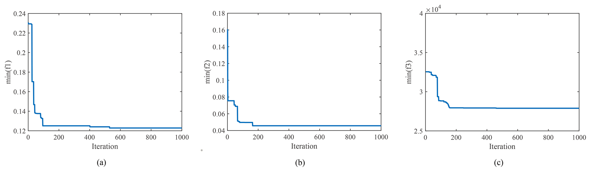
Figure 6 Minimum value of objective functions during iteration. (a) Angular velocity. (b) Joint jerk. (c) Energy.

Figure 7 Pareto front.

5 Trajectory planning based on multi-objective optimization

It is difficult to find a global minimum solution for multi-objective optimization problems (MOPs). In MOP (Liu et al., 2015), a vector ξ dominates ${\mathit{\xi }}^{\ast }(\mathit{\xi }\succ {\mathit{\xi }}^{\ast })$ when the following Pareto dominance principle is satisfied.

$$\begin{array}{}\text{(24)}& \begin{array}{ll}{f}_i\left(\mathit{\xi }\right)\le f_i\left({\mathit{\xi }}^{\ast }\right),& i=\mathrm{1},\mathrm{2},\mathrm{3},\mathrm{\dots },N\\ f_i\left(\mathit{\xi }\right)<f_i\left({\mathit{\xi }}^{\ast }\right),& \exists i\in \mathit{\{}\mathrm{1},\mathrm{2},\mathrm{3},\mathrm{\dots },N\mathit{\}}.\end{array}\end{array}$$

The solution satisfying Eq. (24) is defined as a non-dominated solution of Eq. (22).

Respecting the given multi-objective trajectory optimization problem, the Pareto optimal solution set S is defined as

$$\begin{array}{}\text{(25)}& \left\{S\right\}=\left\{\mathit{\xi }\in \mathbf{\Omega }\left|\mathrm{\neg }\exists {\mathit{\xi }}^{\ast }\in \mathbf{\Omega },{\mathit{\xi }}^{\ast }\succ \mathit{\xi }\right.\right\}.\end{array}$$

The mapping of S is a three-dimensional surface called Pareto front. Therefore, discovering as many non-dominated solutions as possible to cover all features of MOP is the key to solving the proposed trajectory planning problem.

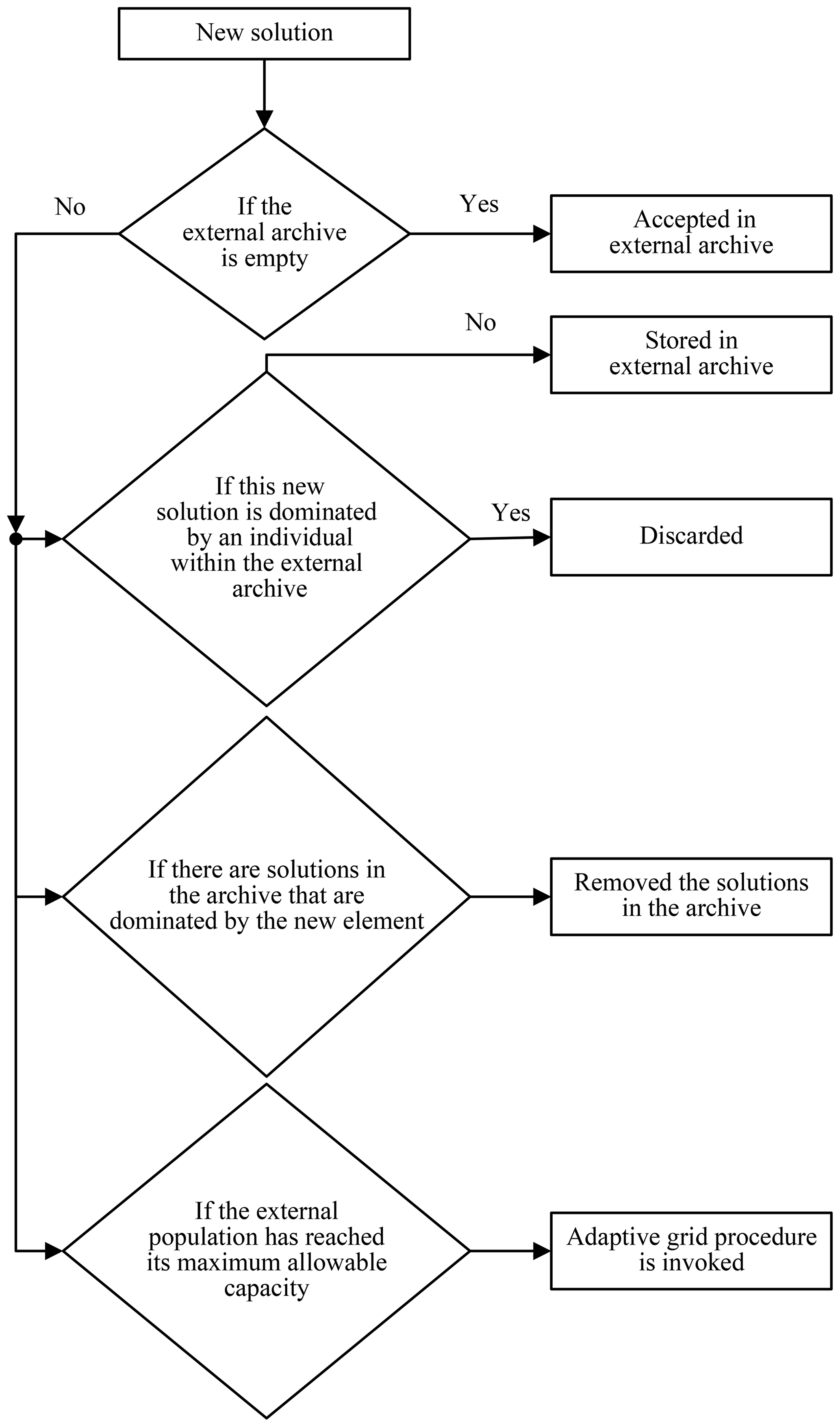
MOPSO algorithm is adopted to solve the multi-objective trajectory optimization problem. This algorithm employs an external repository of particles as guidance to guide the evolution of the whole population toward the Pareto front. Only non-dominated solutions can be stored in the repository according to the following process.

Figure 8 The minimum distances between center of obstacle and manipulator's links.

Figure 9 The configuration change of the manipulator and its geometric relationship with the obstacle. (a) Solution 2. (b) Solution 3.

The velocity formula of particle's flight consists of not only the position and velocity of the current particle (P[k], V[k]) but also the best position that all the particles ever had in the repository (R[h]):

$$\begin{array}{}\text{(26)}& \begin{array}{rl}V\left[k\right]& =\mathit{\chi }\cdot \left[V\right[k]+C_{\mathrm{1}}{R}_{\mathrm{1}}(P_{\mathrm{best}}\left[k\right]-P\left[k\right])\\ & +C_{\mathrm{2}}{R}_{\mathrm{2}}\left(R\right[h]-P[k\left]\right)].\end{array}\end{array}$$

$\mathit{\chi }=\mathrm{2}/(\mathrm{|}\mathrm{2}-\mathit{\varphi }-\sqrt{\mathit{\varphi }(\mathit{\varphi }-\mathrm{4})}\mathrm{|})$ represents the constriction factor; $\mathit{\varphi }=C_{\mathrm{1}}+C_{\mathrm{2}}$, where C₁ and C₂ refer to the learning factors regulating the step size of the particles flying to P_best (the best position a particle has ever explored) and the best position that all the particles ever had, respectively; R₁ and R₂ indicate independent random numbers in the range [0,1].

Combining with the trajectory planning algorithm and MOPSO mentioned above, the obstacle avoidance trajectory optimization can be concluded as follows.

1. The population containing n_P particles is initialized, and the range of decision variables is defined as [T_min,T_max] and [φ_min,φ_max]. Decision variables ξ are randomly generated, and the trajectory of the end effector is calculated by Eq. (1).

2. The joint trajectories are solved according to inverse kinematics, and then the values of three objective functions are obtained following kinematics and dynamics calculation results.

3. The repository is initialized, and its maximum allowable number is restricted to n_R. Next, the positions of particles that represent non-dominated decision vectors in the initial population are stored. Then, the best positions that the particles have had are initialized.

4. While the maximum number of I_max has not been reached, evolutionary computations are performed to update and maintain the repository. The velocities of particles are calculated using Eq. (26), and the position of each particle is updated. Besides, particles that failed to avoid the obstacle are eliminated. The reserved solutions are added into the repository according to the process as shown in Fig. 4. The loop counter is incremented until the maximum number is reached.

5. The non-dominated solutions are obtained from the repository. The particles constitute the set of non-dominant solution S in this paper.

Table 2 Decision vectors and objective vectors of S₂ and S₃.

6 Simulation results and analysis

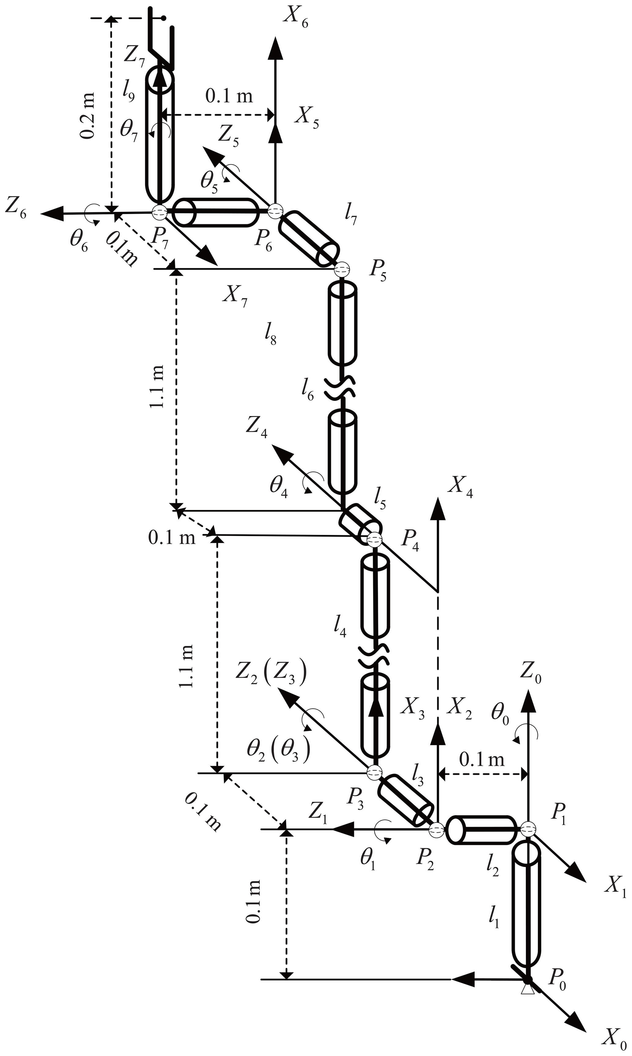
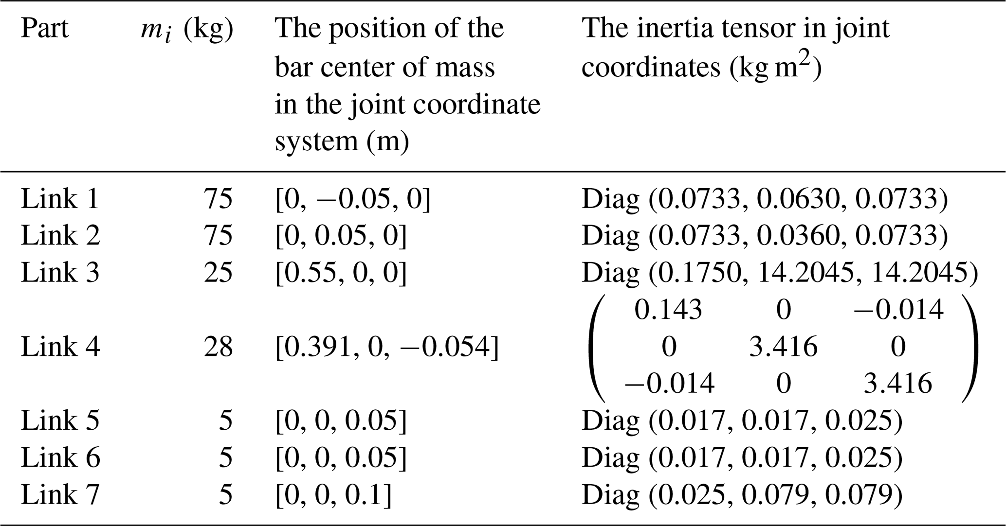
In this paper, a 7-DOF redundant manipulator is adopted to simulate the approached algorithm. The parameters are exhibited in Fig. 5. Mass parameters are provided in Table 1.

The initial configuration of the manipulator is ${\mathit{q}}_{\mathrm{ini}}=[\mathrm{0},\mathrm{0},\mathrm{0},\mathrm{0},\mathrm{0},\mathrm{0},\mathrm{0}{}^{\circ }]$. The corresponding pose of the end effector is ${\mathit{X}}_{\mathrm{ini}}=[-\mathrm{0.5},-\mathrm{0.2},\mathrm{4.6}\mathrm{m},\mathrm{0},\mathrm{0},\mathrm{0}{}^{\circ }]$. The desired pose of the end effector is ${\mathit{X}}_{\mathrm{des}}=[-\mathrm{1.50},\mathrm{1.20},\mathrm{3.60}\mathrm{m},\mathrm{78},-\mathrm{73},-\mathrm{90}{}^{\circ }]$. The total time of motion is t_f=40 s. The upper and lower limits of joint $i(i=\mathrm{1},\mathrm{2},\mathrm{\dots },\mathrm{7})$ are $q_{i\min }=-\mathrm{100}$ and $q_{i\max }=\mathrm{100}{}^{\circ }$, respectively. The radius of link i is r_i=0.1 m. The radius of joint envelope sphere is $r_i^j=\mathrm{0.1}$ m. The obstacle is a sphere whose radius is r_S=0.2 m. The center of the obstacle is located in ${\mathit{Z}}_{\mathrm{0}}=[-\mathrm{0.5},\mathrm{0.3},\mathrm{1.25}\mathrm{m}]$. Scale factors in Eq. (16) are λ₁=0.01 and λ₂=10. The parameters of MOPSO are set as $[{\mathit{\lambda }}_{min\mathrm{1}}^{\prime },{\mathit{\lambda }}_{max\mathrm{1}}^{\prime }]=[+\mathrm{10}\times {\mathrm{10}}^{\mathrm{2}},+\mathrm{10}\times {\mathrm{10}}^{\mathrm{3}}]$, $[{\mathit{\lambda }}_{min\mathrm{2}}^{\prime },{\mathit{\lambda }}_{max\mathrm{2}}^{\prime }]=[-\mathit{\pi },+\mathit{\pi }]$, n_P=1000; n_R=1500; $C_{\mathrm{1}}=C_{\mathrm{2}}=\mathrm{2.05}$.

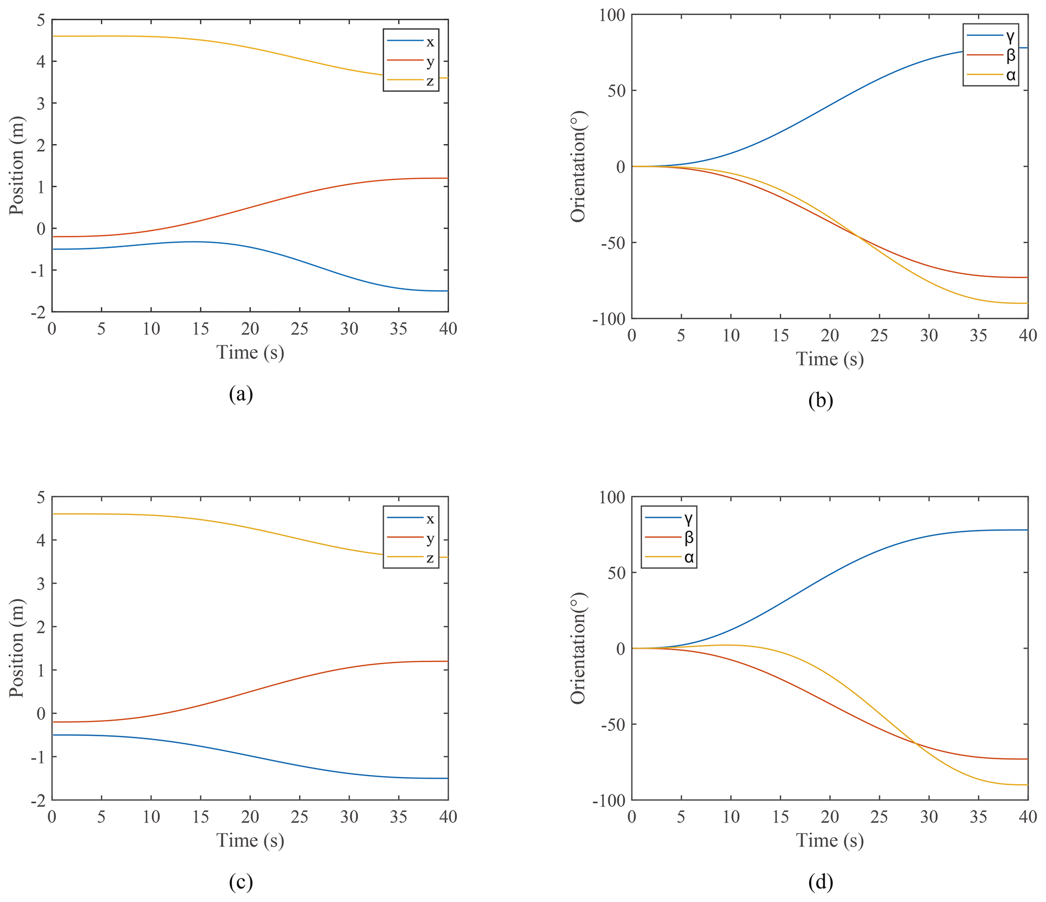
Figure 10 The position and orientation change of end effector. (a) The position changes of end effector in solution 2. (b) The orientation changes of end effector in solution 2. (c) The position changes of end effector in solution 3. (d) The orientation changes of end effector in solution 3.

Figure 11 The change of joint angular. (a) Solution 2. (b) Solution 3.

Figure 12 The change of joint angular velocities. (a) Solution 2. (b) Solution 3.

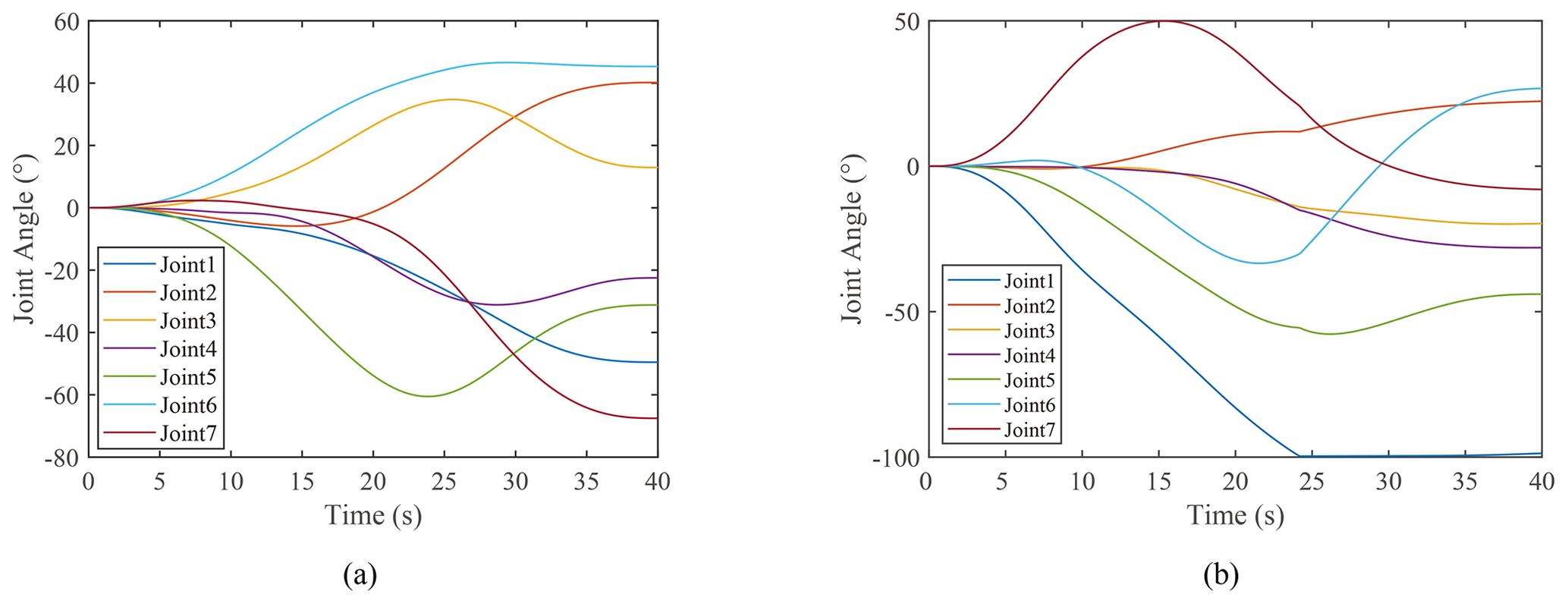
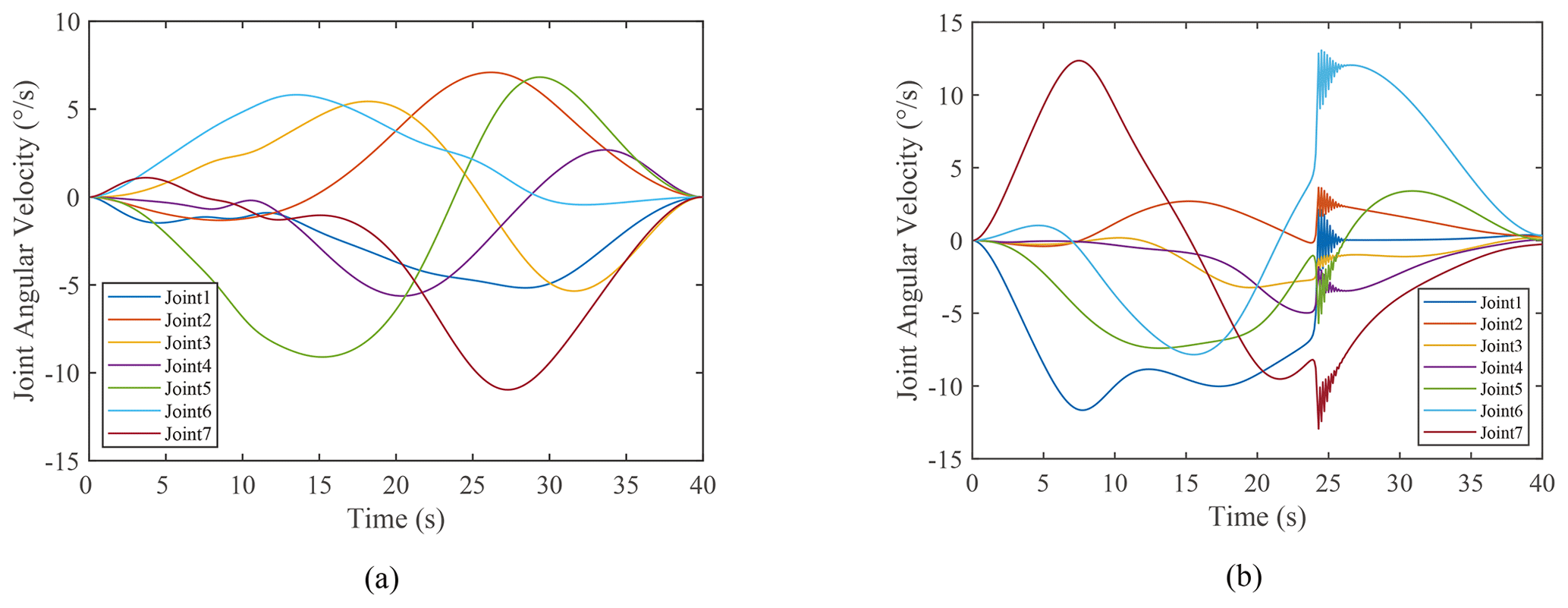
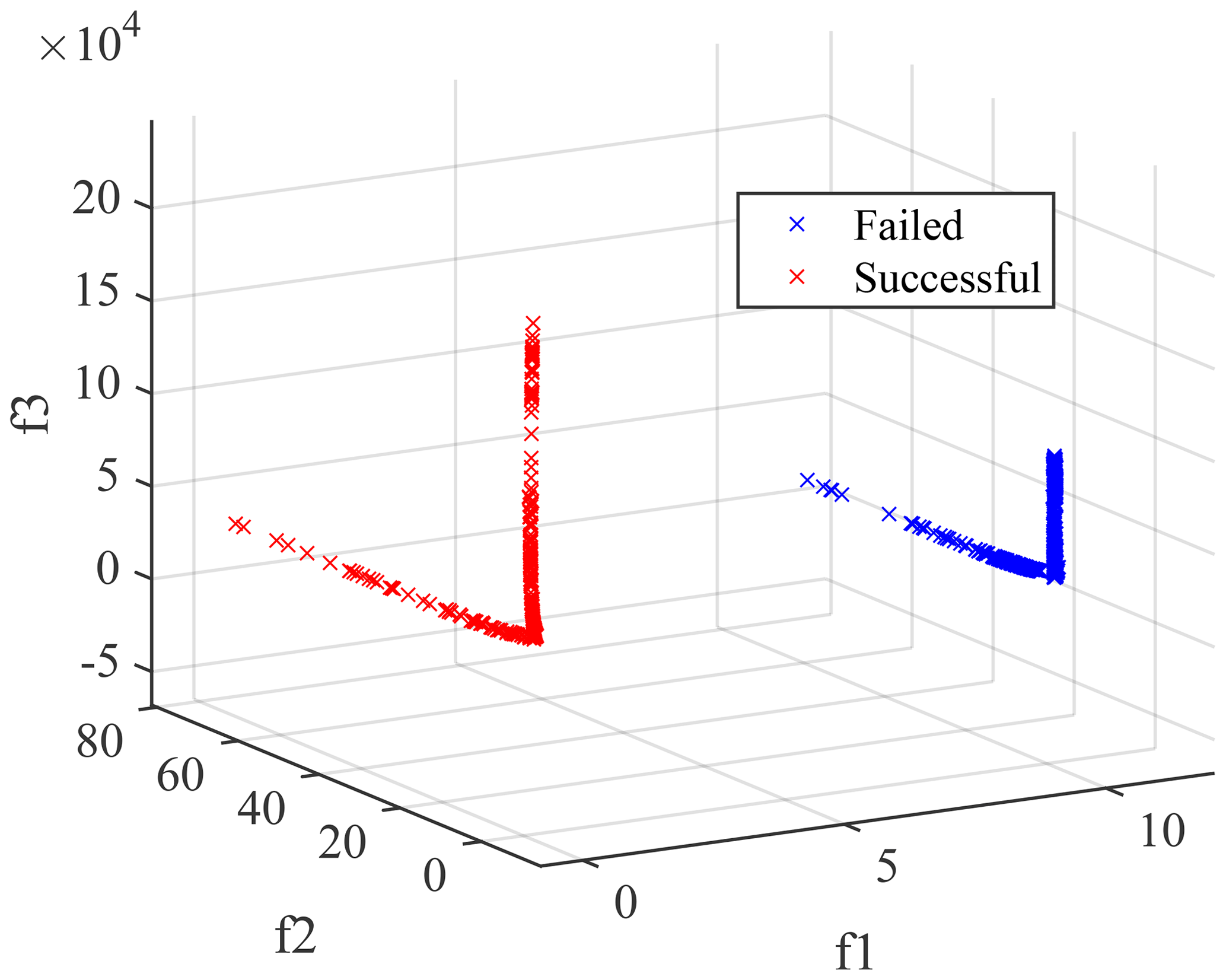
Figure 6 illustrates the minimum value of three objective functions during the iteration, which demonstrates the excellent astringency and stability of the proposed algorithm. The Pareto front is exhibited in Fig. 7. The particles are divided into two categories owing to the penalty function. Red particles satisfy the obstacle avoidance constraint while blue ones do not. Although the screening process can be executed to remove all blue solutions in each iteration, they are reserved to demonstrate the effectiveness of trajectory optimization for obstacle avoidance in this paper. According to the obstacle avoidance constraint, all the remaining non-dominant solutions successfully avoid the obstacle after the particles that fail to avoid the obstacle are removed. This reflects that the proposed algorithm has a good performance in obstacle avoidance.

The first objective function is merely adopted to avoid singularity and obstacles. It will not affect the other physical performance of the redundant manipulator. Therefore, only f₂ and f₃ are considered in the solution selection. The extreme values of cost functions are $f_{\mathrm{2}}^{\min }=\mathrm{0.06}\mathit{\%}{f}_{\mathrm{2}}^{\max }$ and $f_{\mathrm{3}}^{\min }=\mathrm{13.41}\mathit{\%}{f}_{\mathrm{3}}^{\max }$, the specific values are $f_{\mathrm{2}}^{\min }=\mathrm{0.05}$, $f_{\mathrm{2}}^{\max }=\mathrm{76.22}$, $f_{\mathrm{3}}^{\min }=\mathrm{2.79}\times {\mathrm{10}}^{\mathrm{4}}$ and $f_{\mathrm{3}}^{\max }=\mathrm{2.08}\times {\mathrm{10}}^{\mathrm{5}}$. The jerks and energy costs corresponding to different end trajectories significantly vary, verifying the necessity of trajectory optimization.

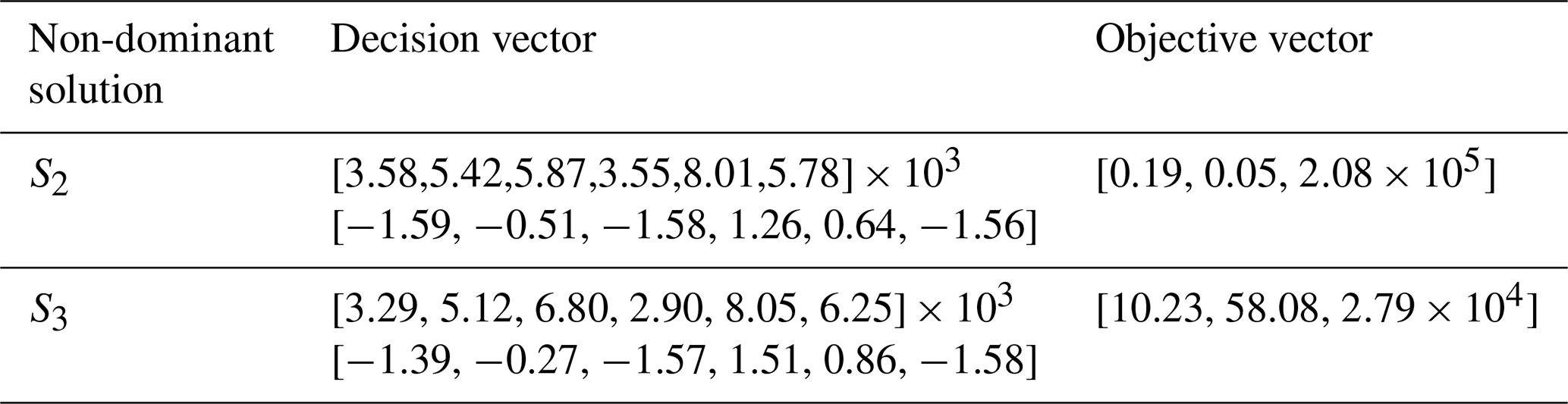
Given no optimal solution to the multi-objective optimization problem, all the solutions are non-dominant. In this paper, the non-dominant solutions corresponding to the minimum values of f₂ and f₃ are selected for comparative analysis. It is assumed that the non-dominant solutions are S₂ and S₃. The decision vectors and objective vectors of S₂ and S₃ are presented in Table 2.

The minimum distances d_i between the center of obstacles and the manipulator's links are illustrated in Fig. 8. The minimum distances for S₂ and S₃ are 0.0597 and 0.0014 m, respectively. The trajectory obtained in S₂ and S₃ successfully avoided the obstacle. The configuration change of the manipulator and its geometric relationship with the obstacle are displayed in Fig. 9. The position and orientation change in the end effector are shown in Fig. 10. The manipulator reached the desired pose with different changing processes.

The change in joint angular over time is exhibited in Fig. 11. Since the joint angular velocity is one of the optimization objectives, no mutation of joint angle occurs. The change in joint angle is smooth. Moreover, the variation range of joint angle is also inhibited with the suppression of joint angular velocity. For solution S₃, the joint angle of link i is still suppressed due to the null-space term, though it approaches the limitation at 24 s. Figure 12 provides the change in joint angular velocities. For S₃, the joint angular velocity changes abruptly when the joint angle approaches the joint limit, forcing the joint angle of the manipulator to return to the range of the joint limit. This also validates the effectiveness of the null-space term as the joint angle constraint in this paper. The shaking process endured for 2 s and finally stabilized. Besides, lower energy cost always demands higher joint jerk, according to Fig. 7. It takes more energy to achieve a smooth angular velocity change, which reduces the impact on the joint mechanisms for redundant manipulators.

7 Conclusions

In this paper, a method of obstacle avoidance trajectory planning based on a multi-objective optimization algorithm in Cartesian space is proposed to avoid obstacles during the redundant manipulator's motion. On the premise that the end effector reaches the desired position and orientation at a specific time, obstacle avoidance can be achieved successfully, and joint jerk and energy consumption can also be inhibited. The results are described as follows.

1. The cosine polynomial function was employed to realize the task requirements of the end effector reaching the desired pose at a specific time. Then, the inverse kinematics and null space inverse solution were introduced to meet the joint angle limit constraint.

2. The multinomial weighted objective function is established in a combination of joint velocity and obstacle avoidance function. By optimizing the proposed function, the manipulator avoids not only the obstacle, but also the joint singularity.

3. Multi-objective particle swarm optimization was performed to optimize joint jerk and energy consumption simultaneously. The clear physical meaning of the objective functions is beneficial for the selection of non-dominant solutions.

The trajectory optimization method proposed in this paper possesses the strong flexibility and diversity. Obstacle avoidance trajectories can be obtained by inputting the initial and expected pose of the end effector. Several non-dominant solutions can be provided for selection. Therefore, this method has an acceptable prospect in engineering applications. However, the collision detection in this paper was implemented based on static obstacles, with all known environment variables. Thus, how to realize dynamic obstacle avoidance in an unknown environment needs to be investigated in the future.