Analysis of divergent bifurcations in the dynamics of wheeled vehicles

This paper presents the bifurcation approach to analyze divergent loss of stability of the symmetric solution of a nonlinear dynamic model in Lyapunov's critical case of a single zero root. Under such a condition, material birth-annihilation bifurcations of multiple stationary states take place. Moreover, the equilibrium surface of stationary states in a small neighborhood of the symmetric solution is a generalized Whitney fold. In the simplest case of a fold peculiarity, the corresponding bifurcation manifold locally coincides with the discriminant manifold of a third-degree polynomial that determines the manifold of stationary states in a small neighborhood of the symmetric solution.

An algorithm to construct the corresponding polynomial is introduced. Through the algorithm, the bifurcation manifold is determined, and the conditions for safe/unsafe loss of stability of the symmetric solution are derived analytically.

The proposed approach to analyze divergent loss of stability is implemented for a nonlinear bicycle model of a two-axle wheeled vehicle. It represents a further development of Pevzner–Pacejka's well-known graph-analytical method. The paper determines the critical values of constructive parameters that are responsible for safe/unsafe loss of stability of the vehicle's straight-line motion, and it discusses strategies for the bifurcation approach to analyze divergent loss of stability.

1 Introduction

The graph-analytical method (Pevzner, 1947) is the first example of qualitative analysis of divergent loss of stability of the nonlinear model of a two-axle vehicle, and it illustrated the main peculiarities of the bifurcation method. Approximately 25 years later, Pacejka (1973a, b, c) re-ignited interest in the graph-analytical method that allowed the stability analysis of the whole manifold of stationary states to take place without the prior determination of the manifold itself. Pacejka (1973a, b, c) recognized the significant potential of the approach of Pevzner (1947), and he actively developed it with the tools that became available in the digital era. He contributed to popularizing the method, and he expanded it with the corresponding database known as the famous “Magic Formula” and its modifications (Pacejka and Besselink, 2012). Nevertheless, subsequent research focused primarily on numerical algorithms to investigate vehicles' stability and determine their bifurcation manifolds (Troger and Zeman, 1984; Kwatny et al., 2003; Della Rossaa et al., 2012; Chen et al., 2016; Sun and He, 2017), even though the graph-analytical method (Verbitskii and Lobas, 1981; Verbitskii et al., 2018; Bobier-Tiu et al., 2019; Jazar et al., 2020) and its extension to the tractor-semitrailer model (Pauwelussen, 2001; Ren et al., 2012) were sporadically applied. These applications unfortunately did not get much attention. We believe that the main obstacle to a wider usage of the graph-analytical method was the inability to apply analytical methods within it.

The paper presents a solution to overcome this obstacle. Specifically, the way forward is to use the functions that are inverted with respect to nonlinear dependencies of side forces along the axles. This makes it possible to utilize the bifurcation method and to obtain an analytical expression for the bifurcation manifold of stationary states of the vehicle's model in the vicinity of the straight-line motion (Verbitskii and Lobas, 1994).

As the theory of continuous projections states (Poston and Stewart, 1980; Arnold, 2012), the “geometry” of a surface of stationary states determines the contours of a bifurcation diagram, when the surface gets projected onto the plane of control parameters with only the multiple points of the surface creating the projection (Fig. 2a). Accordingly, the bifurcation diagram is a graph of critical values of control parameters under which divergent loss of stability of the corresponding stationary states takes place. For example, only two types of peculiarities (fold and cusp) can occur on the surface of stationary states in the case of a dynamic system with two control parameters. A smooth curve is the projection of a fold-type surface, and a semi-cubic parabola with a cusp results from the projection of a cusp type surface. The cusp point itself corresponds to the projection of a triple stationary regime. Proceeding with the construction of the bifurcation manifold, we are going to be interested in the conditions under which multiple stationary regimes take place. This requires knowledge of the equilibrium surface of stationary states as a function of a phase variable and control parameters. There is no generalized approach for calculating the surface. Instead, we propose an algorithm to construct a corresponding determining polynomial that approximates the equilibrium surface in the vicinity of the straight-line stationary regime. The discriminant of the determining polynomial defines the bifurcation manifold. It is a semi-cubic parabola ${\left(p/\mathrm{3}\right)}^{\mathrm{2}}+{\left(q/\mathrm{2}\right)}^{\mathrm{3}}$ for a third-degree polynomial $x^{\mathrm{3}}+p\cdot x+q=\mathrm{0}$. The conditions for safe/unsafe loss of stability of the vehicle's straight-line motion are an important issue that is related to the subject of this paper. They are directly connected to stability/instability of the straight-line motion in Alexander Lyapunov's critical case of a single zero root (Liapunov, 1966). Their interpretation in the context of real bifurcations of stationary states is straightforward. An annihilation bifurcation of the stable straight-line motion and two unstable saddle regimes happens under the “unsafe” loss of stability, and a birth bifurcation of two stable circular regimes out of the stable straight-line motion regime occurs under the “safe” loss of stability. In the latter scenario, the symmetric regime itself loses its stability (Andronov et al., 1966; Bautin, 1949).

2 Characteristic peculiarities of the generalized mathematical model of a wheeled vehicle

The models of symmetrical vehicles are characterized by the equivalence of left-right turns. The trivial solution for such systems corresponds to a stationary rectilinear regime. We assume that when $v=v^{+}$, θ=0 there is a divergent loss of stability of the trivial solution of the system:

$$\begin{array}{}\text{(1)}& \left\{\begin{array}{l}\mathrm{d}x/\mathrm{d}t=f\left(x,u\right),x\in R^{\mathrm{2}},\\ \text{where}u=\left\{v,\mathit{\theta }\right\},v\in R_{+},\mathit{\theta }\in R,\\ f\left(-x,v,-\mathit{\theta }\right)=-f\left(x,v,\mathit{\theta }\right),f\left(\mathrm{0},v,\mathrm{0}\right)=\mathrm{0}.\end{array}\right.\end{array}$$

Stability of the zero solution at $v=v^{+}$ (the critical case of a single zero root) is determined by Lyapunov's first non-zero coefficient g₃ (Liapunov, 1966). If g₃<0, the symmetric solution of the system Eq. (1) is asymptotically stable (Lobas, 2001), and the boundary of the stability domain in the parameter space is safe (Verbitskij and Lobas, 1996) – small variations in the system parameters that lead to crossing the safe boundary of stability generate only a limited growth of phase variables in the vicinity of the symmetric solution. In the case g₃>0 the symmetric solution is unstable, and the boundary of the stability domain in the parameter space is dangerous – even small variations of the system parameters that violate the unstable stability boundary in the parameter space lead to an unlimited increase in perturbations of phase variables in the vicinity of the symmetric solution. The reasons for this mechanism will be explained based on the analysis of steady states of the system in the vicinity of the symmetric solution (real bifurcations of steady states).

3 The methodology of the bifurcation approach for analysis of the divergent loss of stability of the generalized model of a wheeled vehicle

We assume that zero is the regular value of the right-hand parts of the system Eq. (1) and, in addition, that they can be approximated as

$$\begin{array}{}\text{(2)}& \left\{\begin{array}{ll}\mathrm{d}{x}_{\mathrm{1}}/\mathrm{d}t=& a{x}_{\mathrm{1}}+b{x}_{\mathrm{2}}+a_{\mathrm{30}}{x}_{\mathrm{1}}^{\mathrm{3}}+a_{\mathrm{21}}{x}_{\mathrm{1}}^{\mathrm{2}}{x}_{\mathrm{2}}\\ & +a_{\mathrm{12}}{x}_{\mathrm{1}}{x}_{\mathrm{2}}^{\mathrm{2}}+a_{\mathrm{03}}{x}_{\mathrm{2}}^{\mathrm{3}}+a_{\mathrm{50}}{x}_{\mathrm{1}}^{\mathrm{5}}+\mathrm{\dots }\\ & \\ \mathrm{d}{x}_{\mathrm{2}}/\mathrm{d}t=& c{x}_{\mathrm{1}}+\mathrm{d}{x}_{\mathrm{2}}+b_{\mathrm{30}}{x}_{\mathrm{1}}^{\mathrm{3}}+b_{\mathrm{21}}{x}_{\mathrm{1}}^{\mathrm{2}}{x}_{\mathrm{2}}\\ & +b_{\mathrm{12}}{x}_{\mathrm{1}}{x}_{\mathrm{2}}^{\mathrm{2}}+b_{\mathrm{03}}{x}_{\mathrm{2}}^{\mathrm{3}}+b_{\mathrm{50}}{x}_{\mathrm{1}}^{\mathrm{5}}+\mathrm{\dots }\end{array}\right.\end{array}$$

Since when $v=v^{+}$, θ=0 there is a divergent loss of stability of the trivial solution (the linear approximation system has one zero eigenvalue), at least certain coefficients of the linear approximation system depend on the parameters v, θ.

Our next step is to present a geometric interpretation of the stability conditions of a stationary regime for the realization of the critical case of a single Lyapunov zero root.

Stationary regimes of the system (singular points) correspond to the intersection points of two curves which are defined by the right parts of the system (Eq. 2), $f_i(x_{\mathrm{1}},x_{\mathrm{2}})=\mathrm{0}$. The critical value of the parameter $v=v^{+}$ corresponds to the zero root of the linear approximation matrix; therefore, at the critical value of the parameter, these curves have the same inclination angles at the origin (the determinant of the matrix of linear terms turns to zero). Indeed, we will solve each of the equations $f_i(x_{\mathrm{1}},x_{\mathrm{2}})=\mathrm{0}$ ($i=\mathrm{1},\mathrm{2}$) in the vicinity of the origin relative to, for example, a variable x₂:

$$\begin{array}{}\text{(3)}& {\displaystyle }{x}_{\mathrm{2}}=F_{\mathrm{1}}\left(x_{\mathrm{1}}\right)=F_{\mathrm{1}}^{\left(\mathrm{1}\right)}\left(\mathrm{0}\right)x_{\mathrm{1}}+{\displaystyle \frac{\mathrm{1}}{\mathrm{3}\mathrm{!}}}{F}_{\mathrm{1}}^{\left(\mathrm{3}\right)}\left(\mathrm{0}\right)x_{\mathrm{1}}^{\mathrm{3}}+\mathrm{\dots }\text{(4)}& {\displaystyle }{x}_{\mathrm{2}}=F_{\mathrm{2}}\left(x_{\mathrm{1}}\right)=F_{\mathrm{2}}^{\left(\mathrm{1}\right)}\left(\mathrm{0}\right)x_{\mathrm{1}}+{\displaystyle \frac{\mathrm{1}}{\mathrm{3}\mathrm{!}}}{F}_{\mathrm{2}}^{\left(\mathrm{3}\right)}\left(\mathrm{0}\right)x_{\mathrm{1}}^{\mathrm{3}}+\mathrm{\dots }\end{array}$$

The slopes of these curves at the origin are set by the relations

$$\begin{array}{}\text{(5)}& {\displaystyle }{\mathit{\gamma }}_{\mathrm{1}}=F_{\mathrm{1}}^{\left(\mathrm{1}\right)}\left(\mathrm{0}\right)=-{\displaystyle \frac{a}{b}}\text{(6)}& {\displaystyle }{\mathit{\gamma }}_{\mathrm{2}}=F_{\mathrm{2}}^{\left(\mathrm{1}\right)}\left(\mathrm{0}\right)=-{\displaystyle \frac{c}{d}}.\end{array}$$

The relative position of the curves Eqs. (3)–(4) at the critical value of the parameter is determined by the coefficients for nonlinear terms of the sequence ($ab-bc=\mathrm{0}\Rightarrow {\mathit{\gamma }}_{\mathrm{1}}={\mathit{\gamma }}_{\mathrm{2}}$)

$$\begin{array}{}\text{(7)}& {\displaystyle }{F}_{\mathrm{1}}^{\left(\mathrm{3}\right)}\left(\mathrm{0}\right)=\mathrm{6}/b^{\mathrm{4}}\left(-a_{\mathrm{30}}{b}^{\mathrm{3}}+\mathrm{3}{a}_{\mathrm{21}}a{b}^{\mathrm{2}}-\mathrm{3}{a}_{\mathrm{12}}{a}^{\mathrm{2}}b+a_{\mathrm{03}}{a}^{\mathrm{3}}\right)\text{(8)}& {\displaystyle }{F}_{\mathrm{2}}^{\left(\mathrm{3}\right)}\left(\mathrm{0}\right)=\mathrm{6}/d^{\mathrm{4}}\left(-b_{\mathrm{30}}{d}^{\mathrm{3}}+\mathrm{3}{b}_{\mathrm{21}}c{d}^{\mathrm{2}}-\mathrm{3}{b}_{\mathrm{12}}{c}^{\mathrm{2}}d+b_{\mathrm{03}}{c}^{\mathrm{3}}\right).\end{array}$$

Keeping the order of curves in subcritical and critical positions corresponds to a safe loss of stability of the zero solution; breaking the order of curves corresponds to a dangerous loss of stability:

$$\begin{array}{}\text{(9)}& g^{\ast }={\left({\mathit{\gamma }}_{\mathrm{1}}-{\mathit{\gamma }}_{\mathrm{2}}\right)}^{\left(-\right)}\left[F_{\mathrm{1}}^{\left(\mathrm{3}\right)}\left(\mathrm{0}\right)-F_{\mathrm{2}}^{\left(\mathrm{3}\right)}\left(\mathrm{0}\right)\right]>\mathrm{0}.\end{array}$$

Divergent stability loss of a steady state is associated with the realization of a multiple stationary regime: in the simplest case of changing the stability of a symmetric solution, a three-fold regime is realized. From the origin, either a pair of stable steady states is born, which is possible while keeping the order of the curves in Eqs. (3) and 4), or a pair of unstable steady states comes to the origin and merges with the stable steady state; this is in violation of the order of the curves in Eqs. (3) and (4). An example of implementing this approach for the tractor–semitrailer model is presented in Verbitskij and Lobas (1996).

A formal algebraic approach to the analysis of the stability of a stationary regime in the realization of the critical case of a single Lyapunov zero root (promising from the point of view of algorithmization) gives the opportunity to present bifurcation set in a small neighborhood of the three-fold steady state in an analytical form.

In the system of equations defining steady states, we leave the terms no higher than the third order of smallness:

$$\begin{array}{}\text{(10)}& \left\{\begin{array}{l}a{x}_{\mathrm{1}}+b{x}_{\mathrm{2}}+a_{\mathrm{30}}{x}_{\mathrm{1}}^{\mathrm{3}}+a_{\mathrm{21}}{x}_{\mathrm{1}}^{\mathrm{2}}{x}_{\mathrm{2}}+a_{\mathrm{12}}{x}_{\mathrm{1}}{x}_{\mathrm{2}}^{\mathrm{2}}+a_{\mathrm{03}}{x}_{\mathrm{2}}^{\mathrm{3}}=\mathrm{0}\\ \\ c{x}_{\mathrm{1}}+d{x}_{\mathrm{2}}+b_{\mathrm{30}}{x}_{\mathrm{1}}^{\mathrm{3}}+b_{\mathrm{21}}{x}_{\mathrm{1}}^{\mathrm{2}}{x}_{\mathrm{2}}+b_{\mathrm{12}}{x}_{\mathrm{1}}{x}_{\mathrm{2}}^{\mathrm{2}}+b_{\mathrm{03}}{x}_{\mathrm{2}}^{\mathrm{3}}=\mathrm{0}.\end{array}\right.\end{array}$$

Let us proceed from the system of Eq. (10) to a single determining equation, keeping only the terms to the third order of smallness. From the first equation of the system (Eq. 10), we have

$$\begin{array}{}\text{(11)}& \begin{array}{rl}{x}_{\mathrm{1}}& =-a/b{x}_{\mathrm{2}}+(-a_{\mathrm{30}}{b}^{\mathrm{3}}+a_{\mathrm{03}}{a}^{\mathrm{3}}-a_{\mathrm{12}}{a}^{\mathrm{2}}b\\ & +a_{\mathrm{21}}a{b}^{\mathrm{2}})/b^{\mathrm{4}}{x}_{\mathrm{2}}^{\mathrm{3}}+\mathrm{\dots },\end{array}\end{array}$$

and substituting this solution in the second line of Eq. (10), we get a “shortened” defining equation:

$$\begin{array}{}\text{(12)}& \mathit{\gamma }{x}^{\mathrm{3}}+\mathit{\beta }x+\mathit{\alpha }=\mathrm{0},\end{array}$$

where β=β(v), and the function α(θ) characterizes the system's asymmetry when θ≠0. The projection of a critical set on the parameter plane (α,β) defines a bifurcation set (a semi-cubic parabola). At each point of the critical set (in multiple points of the equilibrium surface), the Jacobian of the system (Eq. 1) vanishes.

Values of the coefficients of Eq. (12) at the critical value of the parameter $v=v^{+}$, ${\mathit{\theta }}^{+}=\mathrm{0}$; ($d=cb/a$):

$$\begin{array}{}\text{(13)}& {\displaystyle }\mathit{\alpha }\left({\mathit{\theta }}^{+}\right)=\mathrm{0}\text{(14)}& {\displaystyle }\mathit{\beta }\left(v^{+}\right)=\mathrm{0}\text{(15)}& {\displaystyle }\begin{array}{rl}{\mathit{\gamma }}^{+}& =[b^{\mathrm{3}}\left(a{d}_{\mathrm{30}}-c{a}_{\mathrm{30}}\right)+a{b}^{\mathrm{2}}\left(c{a}_{\mathrm{21}}-a{b}_{\mathrm{21}}\right)\\ & +a^{\mathrm{2}}b\left(a{b}_{\mathrm{12}}-c{a}_{\mathrm{21}}\right)+a^{\mathrm{3}}\left(c{a}_{\mathrm{03}}-a{b}_{\mathrm{03}}\right)/a{b}^{\mathrm{3}}]\end{array}.\end{array}$$

For subcritical values of the parameters $v=v^{+}-\mathit{\epsilon }$, $\mathit{\theta }={\mathit{\theta }}^{+}$, Eq. (12) has the form

$$\begin{array}{}\text{(16)}& \mathit{\gamma }\left(v^{+}-\mathit{\epsilon }\right)x_{\mathrm{2}}^{\mathrm{3}}+\mathit{\beta }\left(v^{+}-\mathit{\epsilon }\right)x_{\mathrm{2}}=\mathrm{0},\end{array}$$

and for a supercritical value $v=v^{+}+\mathit{\epsilon }$, $\mathit{\theta }={\mathit{\theta }}^{+}$,

$$\begin{array}{}\text{(17)}& \mathit{\gamma }\left(v^{+}+\mathit{\epsilon }\right)x_{\mathrm{2}}^{\mathrm{3}}+\mathit{\beta }\left(v^{+}+\mathit{\epsilon }\right)x_{\mathrm{2}}=\mathrm{0}.\end{array}$$

Provided that $\mathit{\gamma }\left(v^{+},{\mathit{\theta }}^{+}\right)\ne \mathrm{0}$, and provided a small enough ε, we will have $\mathit{\gamma }\left(v^{+}-\mathit{\epsilon }\right)\cdot \mathit{\gamma }\left(v^{+}+\mathit{\epsilon }\right)>\mathrm{0}$ and $\mathit{\beta }\left(v^{+}-\mathit{\epsilon }\right)\cdot \mathit{\beta }\left(v^{+}+\mathit{\epsilon }\right)<\mathrm{0}$. This makes it possible to assert that when $v=v^{+}+\mathit{\epsilon }$, $\mathit{\theta }={\mathit{\theta }}^{+}$, there is a cusp bifurcation (three-fold stationary regime is realized), depending on the ratio of the coefficient γ(v⁺) and $\mathit{\beta }\left(v^{+}-\mathit{\epsilon }\right)$ signs: $\mathit{\gamma }\left(v^{+}\right)\cdot \mathit{\beta }\left(v^{+}-\mathit{\epsilon }\right)<\mathrm{0}$ – there is a merge of singular points at the origin; and $\mathit{\gamma }\left(v^{+}\right)\cdot \mathit{\beta }\left(v^{+}-\mathit{\epsilon }\right)>\mathrm{0}\Rightarrow \mathit{\gamma }\left(v^{+}\right)\cdot \mathit{\beta }\left(v^{+}+\mathit{\epsilon }\right)<\mathrm{0}$ – there is a birth of a pair of steady states at the origin.

Using information about the stability state of a symmetric solution ($v<v^{+}$, θ=0, i.e., stability (node); $v>v^{+}$, θ=0, i.e., instability (saddle)), it can be argued that in the case of the merger bifurcation ($\mathit{\gamma }\left(v^{+}\right)\cdot \mathit{\beta }\left(v^{+}-\mathit{\epsilon }\right)<\mathrm{0}$), a pair of saddle singular points comes to the origin, i.e., the corresponding symbolic reaction $O^{\mathrm{2},\mathrm{0}}+(O_{\mathrm{1}}^{\mathrm{1},\mathrm{1}},O_{\mathrm{2}}^{\mathrm{1},\mathrm{1}})\Rightarrow O^{\mathrm{1},\mathrm{1}}$. In the case of birth bifurcation ($\mathit{\gamma }\left(v^{+}\right)\cdot \mathit{\beta }\left(v^{+}-\mathit{\epsilon }\right)>\mathrm{0}$), a pair of singular points with the Poincaré index +1 comes out of the symmetric solution (origin), i.e., a symbolic reaction (Andronov et al., 1966):

$$\begin{array}{}\text{(18)}& O^{\mathrm{2},\mathrm{0}}\Rightarrow O^{\mathrm{1},\mathrm{1}}+(O_{\mathrm{1}}^{\mathrm{2},\mathrm{0}},O_{\mathrm{2}}^{\mathrm{2},\mathrm{0}}).\end{array}$$

The merger bifurcation corresponds to instability in the critical case and dangerous loss of stability in the sense of Bautin (1949) (at subcritical speed $v=v^{+}-\mathit{\epsilon }$, a pair of saddle singular points narrow the pool of attraction of a symmetrical solution, and at $v=v^{+}+\mathit{\epsilon }$, the symmetric solution corresponds to an isolated “saddle”, so the perturbations of phase variables grow unlimitedly). Bifurcation of birth corresponds to stability in the critical case and safe loss of stability in the sense of Nikolai Bautin (at subcritical speed $v=v^{+}-\mathit{\epsilon }$, the symmetric solution corresponds to an isolated stable “node”, and at supercritical speed $v=v^{+}+\mathit{\epsilon }$, in the small neighborhood of the saddle there are two stable singular points that limit the growth of perturbations of phase variables).

Up to a constant multiplier, Lyapunov's coefficient determining the stability of the zero solution of the system (Eq. 2) in the critical case of a single zero root coincides with the coefficient (Liapunov, 1966; Lobas, 2001).

4 An example of divergent loss of stability in a nonlinear model of a wheeled vehicle

Let us consider a single mass “bicycle” model of a vehicle with fixed steering (Ellis, 1975; Gillespie, 1992) as represented in Fig. 1.

Figure 1 The vehicle's model.

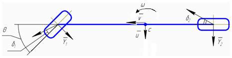
The model's equations of motion are as follows:

$$\begin{array}{}\text{(19)}& \left\{\begin{array}{l}m\left(\dot{u}+v\mathit{\omega }\right)=Y_{\mathrm{1}}\left({\mathit{\delta }}_{\mathrm{1}}\right)\cos \mathit{\theta }+Y_{\mathrm{2}}\left({\mathit{\delta }}_{\mathrm{2}}\right)\\ J\dot{\mathit{\omega }}=a{Y}_{\mathrm{1}}\left({\mathit{\delta }}_{\mathrm{1}}\right)\cos \mathit{\theta }-b{Y}_{\mathrm{2}}\left({\mathit{\delta }}_{\mathrm{2}}\right)\end{array}\right.,\end{array}$$

where v are u are the longitudinal and transverse projections of the velocity vector of the vehicle's center of mass onto the vehicle's axes; θ is the angle of rotation of the wheeled unit; ω is the angular velocity around the vertical axis; m and J are the mass and the central moment of inertia; a and b are the distances between the vehicle's center of mass and the centers of the vehicle's front (controlled) and back axles; and $l=a+b$ is the base of the vehicle.

The stationary states can be determined as the solutions of a finite nonlinear system:

$$\begin{array}{}\text{(20)}& \begin{array}{l}mv\mathit{\omega }=Y_{\mathrm{1}}\left({\mathit{\delta }}_{\mathrm{1}}\right)\cos \mathit{\theta }+Y_{\mathrm{2}}\left({\mathit{\delta }}_{\mathrm{2}}\right)\\ \mathrm{0}=a{Y}_{\mathrm{1}}\left({\mathit{\delta }}_{\mathrm{1}}\right)\cos \mathit{\theta }-b{Y}_{\mathrm{2}}\left({\mathit{\delta }}_{\mathrm{2}}\right).\end{array}\end{array}$$

The side force dependencies Y₁(δ₁)Y₂(δ₂) are nonlinear functions of slipping angles that are determined by approximate linear relations (we are also going to assume cos θ≈1):

$$\begin{array}{}\text{(21)}& {\displaystyle }{\mathit{\delta }}_{\mathrm{1}}=\mathit{\theta }-{\displaystyle \frac{u+a\mathit{\omega }}{v}}\text{(22)}& {\displaystyle }{\mathit{\delta }}_{\mathrm{2}}={\displaystyle \frac{-u+b\mathit{\omega }}{v}}.\end{array}$$

Defining ${\stackrel{\mathrm{‾}}{Y}}_i=Y_i/N_i$ as the dimensionless side forces, where $N_i(i=\mathrm{1},\mathrm{2})$: $N_{\mathrm{1}}=\frac{mgb}{l}$, $N_{\mathrm{2}}=\frac{mga}{l}$ are the surface's vertical reaction forces on the vehicle's axles, we transform the system (Eq. 20) to a dimensionless representation:

$$\begin{array}{}\text{(23)}& {\displaystyle \frac{v\mathit{\omega }}{g}}=\stackrel{\mathrm{‾}}{Y_{\mathrm{1}}}{\displaystyle \frac{b}{l}}+\stackrel{\mathrm{‾}}{Y_{\mathrm{2}}}{\displaystyle \frac{a}{l}}\text{(24)}& {\displaystyle }\stackrel{\mathrm{‾}}{Y_{\mathrm{1}}}-\stackrel{\mathrm{‾}}{Y_{\mathrm{2}}}=\mathrm{0},\end{array}$$

and it can be reduced to a single defining equation.

The side forces that occur in the stationary circular states are found qualitatively as the solution to the linear system of Eqs. (23)–(24):

$$\begin{array}{}\text{(25)}& \stackrel{\mathrm{‾}}{Y_{\mathrm{1}}}=\stackrel{\mathrm{‾}}{Y_{\mathrm{2}}}=\stackrel{\mathrm{‾}}{Y};\stackrel{\mathrm{‾}}{Y}={\displaystyle \frac{v\mathit{\omega }}{g}}=\stackrel{\mathrm{‾}}{a_y},\end{array}$$

where $\stackrel{\mathrm{‾}}{a_y}$ is the vehicle's dimensionless side acceleration in the stationary circular state, that is the projection of the centripetal acceleration onto the transverse axes.

Next, we switch to $\stackrel{\mathrm{‾}}{Y}$: ${\mathit{\delta }}_{\mathrm{1}}=G_{\mathrm{1}}\left(\stackrel{\mathrm{‾}}{Y}\right)$, ${\mathit{\delta }}_{\mathrm{2}}=G_{\mathrm{2}}\left(\stackrel{\mathrm{‾}}{Y}\right)$, where ${\mathit{\delta }}_i=G_i\left(\stackrel{\mathrm{‾}}{Y}\right)$ denotes the inverse functions of ${\stackrel{\mathrm{‾}}{Y}}_i={\stackrel{\mathrm{‾}}{Y}}_i\left({\mathit{\delta }}_i\right)$. From the definition of slipping angles, we obtain

$$\begin{array}{}\text{(26)}& \mathit{\omega }={\displaystyle \frac{v\left(\mathit{\theta }+{\mathit{\delta }}_{\mathrm{2}}-{\mathit{\delta }}_{\mathrm{1}}\right)}{l}}.\end{array}$$

Taking the above into account, we derive the defining equation from the first equation of the system (23)–(24). It is either

$$\begin{array}{}\text{(27)}& {\displaystyle \frac{v^{\mathrm{2}}}{gl}}\left(\mathit{\theta }+{\mathit{\delta }}_{\mathrm{2}}-{\mathit{\delta }}_{\mathrm{1}}\right)=\stackrel{\mathrm{‾}}{Y}\left({\mathit{\delta }}_{\mathrm{2}}-{\mathit{\delta }}_{\mathrm{1}}\right)\end{array}$$

or

$$\begin{array}{}\text{(28)}& G\left(\stackrel{\mathrm{‾}}{Y}\right)={\displaystyle \frac{gl}{v^{\mathrm{2}}}}\stackrel{\mathrm{‾}}{Y}-\mathit{\theta },\end{array}$$

where the function $G\left(\stackrel{\mathrm{‾}}{Y}\right)=G_{\mathrm{2}}\left(\stackrel{\mathrm{‾}}{Y}\right)-G_{\mathrm{1}}\left(\stackrel{\mathrm{‾}}{Y}\right)$. It is these two relations that determine the equilibrium surface for the δ₂−δ₁ or $\stackrel{\mathrm{‾}}{Y}$ phase variables. Both are tied to the phase variable ω, which is the critical variable in our case, and they differ by a constant multiplier.

Equation (28) is better suited, as it allows us to obtain the defining polynomial analytically if the side force dependencies are analytically given. It is impossible in the case of Eq. (27) since $\stackrel{\mathrm{‾}}{Y}\left({\mathit{\delta }}_{\mathrm{2}}-{\mathit{\delta }}_{\mathrm{1}}\right)$ is defined graphically (Pacejka, 1980). We will assume that the dimensionless side forces are defined by the following expression, with k_i denoting the dimensionless coefficients of cornering stiffness on the vehicle's axles:

$$\begin{array}{}\text{(29)}& {\displaystyle }{\stackrel{\mathrm{‾}}{Y}}_i=k_i\cdot {\mathit{\delta }}_i/{\left(\mathrm{1}+{\left(k_i\cdot {\mathit{\delta }}_i/{\mathit{\phi }}_i\right)}^{\mathrm{2}}\right)}^{\mathrm{1}/\mathrm{2}}\text{(30)}& {\displaystyle }{\stackrel{\mathrm{‾}}{Y}}_i\approx k_i\cdot {\mathit{\delta }}_i-\mathrm{1}/\mathrm{2}{\left(k_i\cdot {\mathit{\delta }}_i\right)}^{\mathrm{3}}/{\mathit{\phi }}_i^{\mathrm{2}}.\end{array}$$

If we consider a nonlinear approximation of the side forces to the third order of smallness

$$\begin{array}{}\text{(31)}& {\stackrel{\mathrm{‾}}{Y}}_i\approx k_i\cdot {\mathit{\delta }}_i-K_i\cdot {\mathit{\delta }}_i^{\mathrm{3}},\end{array}$$

the inverse functions are

$$\begin{array}{}\text{(32)}& {\mathit{\delta }}_i\approx p_i\cdot \stackrel{\mathrm{‾}}{Y}+P_i\cdot {\stackrel{\mathrm{‾}}{Y}}^{\mathrm{3}},\end{array}$$

with the coefficients $p_i=\frac{\mathrm{1}}{k_i}$; $P_i=\frac{K_i}{k_i^{\mathrm{4}}}$. And the function $G\left(\stackrel{\mathrm{‾}}{Y}\right)=G_{\mathrm{2}}\left(\stackrel{\mathrm{‾}}{Y}\right)-G_{\mathrm{1}}\left(\stackrel{\mathrm{‾}}{Y}\right)$ becomes

$$\begin{array}{}\text{(33)}& G\left(\stackrel{\mathrm{‾}}{Y}\right)\approx \mathrm{1}/k_{\mathrm{2}}\cdot \stackrel{\mathrm{‾}}{Y}+{\stackrel{\mathrm{‾}}{Y}}^{\mathrm{3}}/\left(\mathrm{2}{k}_{\mathrm{2}}{\mathit{\phi }}_{\mathrm{2}}^{\mathrm{2}}\right)-\mathrm{1}/k_{\mathrm{1}}\cdot \stackrel{\mathrm{‾}}{Y}-{\stackrel{\mathrm{‾}}{Y}}^{\mathrm{3}}/\left(\mathrm{2}{k}_{\mathrm{1}}{\mathit{\phi }}_{\mathrm{1}}^{\mathrm{2}}\right).\end{array}$$

Therefore, the conditions for safe/unsafe loss of stability of the stationary straight-line motion are obtained from Eq. (28). Its cubic approximation defines the determining polynomial (Eq. 12):

$$\begin{array}{}\text{(34)}& \begin{array}{rl}& \left[\mathrm{1}/\left(\mathrm{2}{k}_{\mathrm{2}}{\mathit{\phi }}_{\mathrm{2}}^{\mathrm{2}}\right)-\mathrm{1}/\left(\mathrm{2}{k}_{\mathrm{1}}{\mathit{\phi }}_{\mathrm{1}}^{\mathrm{2}}\right)\right]{\stackrel{\mathrm{‾}}{Y}}^{\mathrm{3}}\\ & +\left(-gl/v^{\mathrm{2}}+\mathrm{1}/k_{\mathrm{2}}-\mathrm{1}/k_{\mathrm{1}}\right)\stackrel{\mathrm{‾}}{Y}+\mathit{\theta }=\mathrm{0},\end{array}\end{array}$$

where

$$\begin{array}{}\text{(35)}& {\displaystyle }\mathit{\gamma }=\mathrm{1}/\left(\mathrm{2}{k}_{\mathrm{2}}{\mathit{\phi }}_{\mathrm{2}}^{\mathrm{2}}\right)-\mathrm{1}/\left(\mathrm{2}{k}_{\mathrm{1}}{\mathit{\phi }}_{\mathrm{1}}^{\mathrm{2}}\right)\text{(36)}& {\displaystyle }\mathit{\beta }\left(v\right)=-gl/v^{\mathrm{2}}+\mathrm{1}/k_{\mathrm{2}}-\mathrm{1}/k_{\mathrm{1}}\text{(37)}& {\displaystyle }\mathit{\alpha }=\mathit{\theta }.\end{array}$$

A semi-cubic parabola on the (v, θ) parameter plane, where the discriminant of the cubic Eq. (28) becomes zero, delimits the regions with different numbers of stationary states. In other words, it determines the boundaries of divergent loss of stability in the system's parameter space. The conditions under which the cusp bifurcation of the triple zero state $\mathit{\beta }\left(v^{+}\right)=\mathrm{0}$, $\mathit{\alpha }\left({\mathit{\theta }}^{+}\right)=\mathrm{0}$ unfolds set the coordinates of the tension point.

$$\begin{array}{}\text{(38)}& \left(v^{+}={\left({\displaystyle \frac{k_{\mathrm{1}}{k}_{\mathrm{2}}gl}{k_{\mathrm{1}}-k_{\mathrm{2}}}}\right)}^{\mathrm{1}/\mathrm{2}},{\mathit{\theta }}^{+}=\mathrm{0}\right)\end{array}$$

The critical velocity v⁺ in Eq. (38) coincides with the critical velocity of the straight-line motion that is determined from the linear approximation system of the vehicle's model.

Two-fold stationary regimes (the fold bifurcation) correspond to the regular points of the discriminant manifold (v^∗, θ^∗). They form the boundaries of divergent loss of stability of circular stationary regimes. For example, it is possible to determine the maximum value of the angle of rotation of the controlled module that would ensure the stability of a circular stationary motion for a given velocity v.

4.1 The stability conditions in the critical case (the conditions for safe/unsafe loss of stability à la Bautin)

Let us rewrite the determining polynomial (Eq. 34), as we incorporate the expression for the critical velocity of the straight-line motion v⁺:

$$\begin{array}{}\text{(39)}& \begin{array}{rl}& \left[{\displaystyle \frac{\mathrm{1}}{\left(\mathrm{2}{k}_{\mathrm{2}}{\mathit{\phi }}_{\mathrm{2}}^{\mathrm{2}}\right)}}-{\displaystyle \frac{\mathrm{1}}{\left(\mathrm{2}{k}_{\mathrm{1}}{\mathit{\phi }}_{\mathrm{1}}^{\mathrm{2}}\right)}}\right]{\stackrel{\mathrm{‾}}{Y}}^{\mathrm{3}}\\ & +{\displaystyle \frac{k_{\mathrm{1}}-k_{\mathrm{2}}}{k_{\mathrm{1}}{k}_{\mathrm{2}}}}\left[\mathrm{1}-{\left({\displaystyle \frac{v^{+}}{v}}\right)}^{\mathrm{2}}\right]\stackrel{\mathrm{‾}}{Y}+\mathit{\theta }=\mathrm{0}.\end{array}\end{array}$$

Three stationary regimes take place in the system under $\mathit{\gamma }\left(v^{+}\right)>\mathrm{0}$ and $v<v^{+}$ or $\mathit{\gamma }\left(v^{+}\right)<\mathrm{0}$ and $v>v^{+}$. A merger of critical points occurs in the origin under $\mathit{\gamma }\left(v^{+}\right)\cdot \mathit{\beta }\left(v^{+}-\mathit{\epsilon }\right)<\mathrm{0}$, and as a consequence, the symmetrical solution is unstable in the critical case; that is, unsafe loss of stability à la Bautin (Bautin, 1949) takes place.

Three stationary regimes materialize under $\mathit{\gamma }\left(v^{+}\right)<\mathrm{0}$ and $v>v^{+}$. The birth of a pair of critical states in the origin happens under $\mathit{\gamma }\left(v^{+}\right)\cdot \mathit{\beta }\left(v^{+}-\mathit{\epsilon }\right)>\mathrm{0}\Rightarrow \mathit{\gamma }\left(v^{+}\right)\cdot \mathit{\beta }\left(v^{+}+\mathit{\epsilon }\right)<\mathrm{0}$, and the symmetrical solution is stable in the critical case; that is, safe loss of stability à la Bautin takes place.

Therefore, the conditions for unsafe loss of stability for the vehicle's model under $\mathit{\gamma }\left(v^{+}\right)>\mathrm{0}$ are

$$\begin{array}{}\text{(40)}& {\displaystyle }{k}_{\mathrm{1}}-k_{\mathrm{2}}>\mathrm{0};\text{(41)}& {\displaystyle }{k}_{\mathrm{1}}{\mathit{\phi }}_{\mathrm{1}}^{\mathrm{2}}>k_{\mathrm{2}}{\mathit{\phi }}_{\mathrm{2}}^{\mathrm{2}}.\end{array}$$

The conditions for safe loss of stability under $\mathit{\gamma }\left(v^{+}\right)<\mathrm{0}$: are

$$\begin{array}{}\text{(42)}& {\displaystyle }{k}_{\mathrm{1}}-k_{\mathrm{2}}<\mathrm{0};\text{(43)}& {\displaystyle }{k}_{\mathrm{1}}{\mathit{\phi }}_{\mathrm{1}}^{\mathrm{2}}<k_{\mathrm{2}}{\mathit{\phi }}_{\mathrm{2}}^{\mathrm{2}}.\end{array}$$

The determining polynomial will look somewhat different to the one in Eq. (34) above if we apply the general approach presented in Eqs. (10)–(12). Nevertheless, the conditions for safe/unsafe loss of stability will remain the same.

$$\begin{array}{}\text{(44)}& \begin{array}{rl}& {\displaystyle \frac{v^{\mathrm{2}}}{g\cdot l}}\cdot \left[\left({\displaystyle \frac{\mathrm{1}}{k_{\mathrm{1}}}}+{\displaystyle \frac{g\cdot l}{v^{\mathrm{2}}}}\right)K_{\mathrm{2}}-{\displaystyle \frac{K_{\mathrm{1}}\cdot k_{\mathrm{2}}^{\mathrm{3}}}{k_{\mathrm{1}}^{\mathrm{4}}}}\right]\cdot {\stackrel{\mathrm{‾}}{Y}}^{\mathrm{3}}\\ & +{\displaystyle \frac{v^{\mathrm{2}}\cdot \left(k_{\mathrm{1}}-k_{\mathrm{2}}\right)}{k_{\mathrm{1}}\cdot g\cdot l}}\cdot \left(\mathrm{1}-{\displaystyle \frac{k_{\mathrm{1}}\cdot k_{\mathrm{2}}\cdot g\cdot l}{v^{\mathrm{2}}\cdot \left(k_{\mathrm{1}}-k_{\mathrm{2}}\right)}}\right)\cdot \stackrel{\mathrm{‾}}{Y}\\ & +{\displaystyle \frac{v^{\mathrm{2}}}{g\cdot l}}\mathit{\theta }=\mathrm{0},\end{array}\end{array}$$

where $K_i=\mathrm{1}/\mathrm{2}\cdot k_i^{\mathrm{3}}/{\mathit{\phi }}_i^{\mathrm{2}}$.

The polynomial above can be transformed into

$$\begin{array}{}\text{(45)}& {\displaystyle }\begin{array}{rl}& k_{\mathrm{2}}^{\mathrm{3}}\left({\displaystyle \frac{\mathrm{1}}{\mathrm{2}{k}_{\mathrm{2}}{\mathit{\phi }}_{\mathrm{2}}^{\mathrm{2}}}}-{\displaystyle \frac{\mathrm{1}}{\mathrm{2}{k}_{\mathrm{1}}{\mathit{\phi }}_{\mathrm{1}}^{\mathrm{2}}}}\right){\stackrel{\mathrm{‾}}{Y}}^{\mathrm{3}}\\ & +{\displaystyle \frac{k_{\mathrm{1}}-k_{\mathrm{2}}}{k_{\mathrm{1}}}}\left[\mathrm{1}-{\left({\displaystyle \frac{v^{+}}{v}}\right)}^{\mathrm{2}}\right]\stackrel{\mathrm{‾}}{Y}+\mathit{\theta }=\mathrm{0}\end{array}\text{(46)}& {\displaystyle }\mathit{\gamma }\left(v^{+}\right)=k_{\mathrm{2}}^{\mathrm{3}}\left({\displaystyle \frac{\mathrm{1}}{\mathrm{2}{k}_{\mathrm{2}}{\mathit{\phi }}_{\mathrm{2}}^{\mathrm{2}}}}-{\displaystyle \frac{\mathrm{1}}{\mathrm{2}{k}_{\mathrm{1}}{\mathit{\phi }}_{\mathrm{1}}^{\mathrm{2}}}}\right),\end{array}$$

and it shows that the two approaches do indeed result in the same conditions for safe/unsafe loss of stability.

Figure 2 illustrates the transition from unsafe to safe loss of stability of the straight-line motion of the vehicle, as the cornering stiffness φ₁ decreases. The redrawing of the bifurcation manifold corresponds to the transformation of the cusp surface as the parameter changes.

Figure 2 Changes in the bifurcation manifold as φ₁ decreases.

To better understand it, it is necessary to consider terms up to the fifth degree in Eq. (34).

As Eq. (27) is used in Pevzner–Pacejka's graph-analytical method, we will use it to analyze the number of stationary regimes under a fixed velocity $v<v^{+}$ and the values of the parameter φ₁ that correspond to cases (a), (b) and (c) in Fig. 2.

Figure 3 Stationary regimes under a fixed velocity $v<v^{+}$ and variations in the parameter φ₁.

For case (a), $\mathit{\{}{\mathit{\phi }}_{\mathrm{1}}={\mathit{\phi }}_{\mathrm{2}},k_{\mathrm{1}}\cdot {\mathit{\phi }}_{\mathrm{1}}^{\mathrm{2}}>k_{\mathrm{2}}\cdot {\mathit{\phi }}_{\mathrm{2}}^{\mathrm{2}}\mathit{\}}$. For (b), $\mathit{\{}{\mathit{\phi }}_{\mathrm{1}}<{\mathit{\phi }}_{\mathrm{2}},k_{\mathrm{1}}\cdot {\mathit{\phi }}_{\mathrm{1}}^{\mathrm{2}}>k_{\mathrm{2}}\cdot {\mathit{\phi }}_{\mathrm{2}}^{\mathrm{2}}\mathit{\}}$. 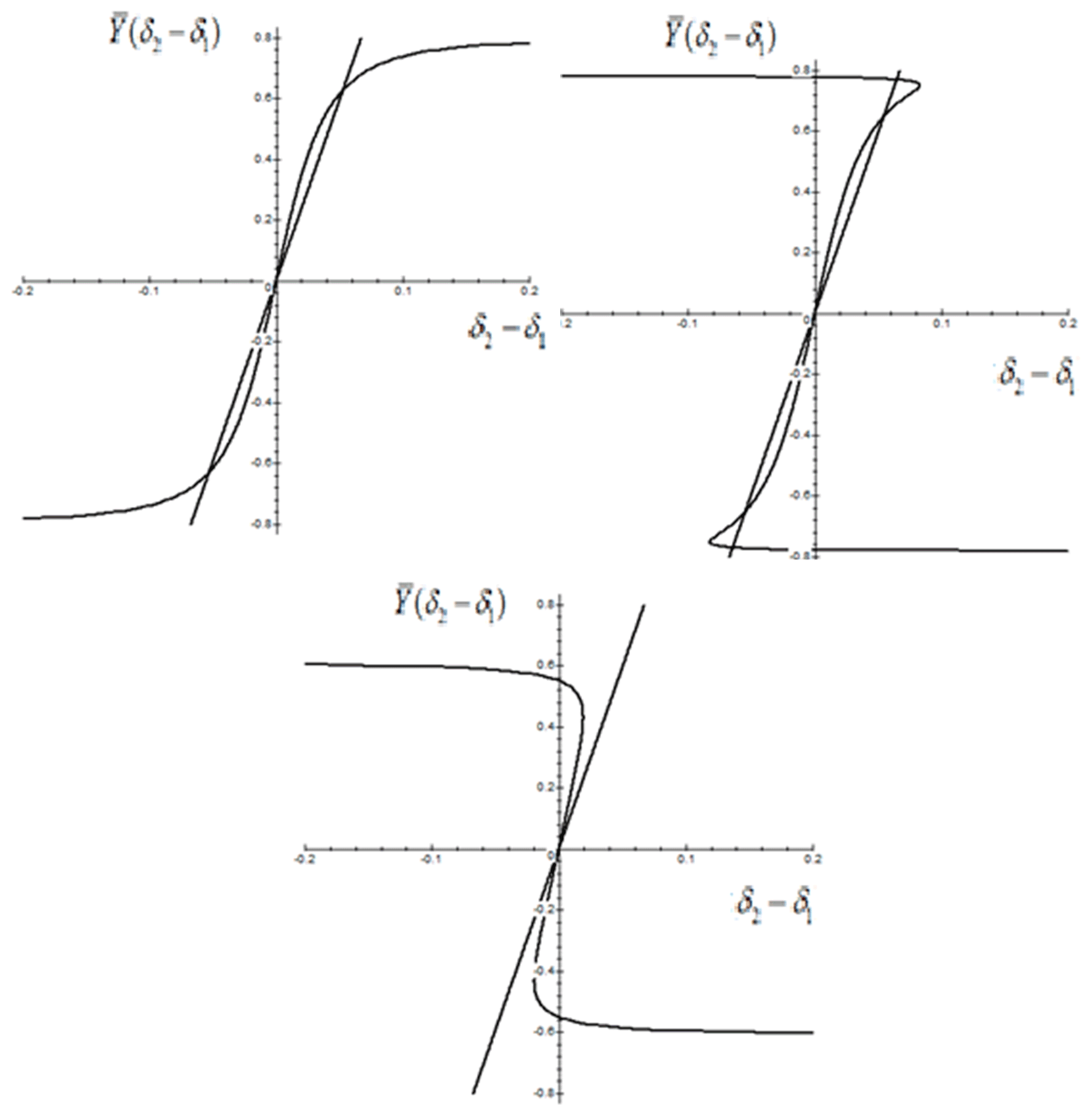For (c), $\mathit{\{}{\mathit{\phi }}_{\mathrm{1}}<{\mathit{\phi }}_{\mathrm{2}},k_{\mathrm{1}}\cdot {\mathit{\phi }}_{\mathrm{1}}^{\mathrm{2}}<k_{\mathrm{2}}\cdot {\mathit{\phi }}_{\mathrm{2}}^{\mathrm{2}}\mathit{\}}$. The parameter φ₁ is smaller than the critical value ${\mathit{\phi }}_{\mathrm{1}}<{\mathit{\phi }}_{\mathrm{1}}^{\ast }=\sqrt[\mathrm{2}]{\frac{k_{\mathrm{2}}{\mathit{\phi }}_{\mathrm{2}}^{\mathrm{2}}}{k_{\mathrm{1}}}}$.

The change in the nature of the stability domain border is connected to the emergence of a “butterfly” catastrophe with a five-fold stationary regime. The additional inflection points in Fig. 3b move to the origin, where the five-fold stationary regime takes place. The cusp points on the bifurcation curve correspond to the inflection points on the curve $\stackrel{\mathrm{‾}}{Y}\left({\mathit{\delta }}_{\mathrm{2}}-{\mathit{\delta }}_{\mathrm{1}}\right)$.

5 Discussion of the strategy for bifurcation analysis of a dynamic system

For a system of equations,

$$\begin{array}{}\text{(47)}& f_i\left(x,\mathit{\theta },v\right)=\mathrm{0},x\in R^n\left(i=\mathrm{1},\mathrm{\dots },n\right),\end{array}$$

the solutions of which determine the set of steady states of a nonlinear dynamic model (the right parts of the equations of motion of the model depend on two scalar parameters). The bifurcation values of the parameters (v^*, θ^*) correspond to multiple solutions x^* of the system Eq. (47). The Jacobian of the system vanishes at all points of the critical set x^*:

$$\begin{array}{}\text{(48)}& \mathbf{J}={∥\mathrm{d}{f}_i/\mathrm{d}{x}_i∥}_{x^{*}}=\mathrm{0},x^{*}\mathit{ϵ}{M}_{\mathrm{kr}}.\end{array}$$

If the rank of the Jacobi matrix is n−1 (there is exactly one zero eigenvalue of the linearization matrix), then the surface of steady states in the vicinity of the corresponding critical point x^* in cases of the “general position” is a fold or cusp. The system shown by Eq. (47), together with Eq. (48), defines a critical set on a manifold of steady states (it is a parametrized smooth curve). Under these assumptions, it will be possible to apply the numerical–analytical method of continuation for two parameters. There is a disappearance of a stable steady state through the fold bifurcation in the points of “turning” (“smooth return points”) of a critical set, and “cusp” (“return point”) corresponds to the change of stability of steady state (in a system with simplest symmetry, this steady state corresponds to the rectilinear regime that loses its stability when θ=0, $v=v^{+}$).

In the presence of small perturbations that violate the symmetry of a dynamic system with two control parameters, the cusp does not disappear (it shifts, losing its symmetry), which is a consequence of structural stability.

Generally speaking, any qualitative changes in the picture of steady states when changing the controllable parameters of the system are associated with the appearance–disappearance of a pair of singular points or in general with the appearance-splitting of a k-fold singular point (real bifurcations). In this case, the surface of steady states (equilibrium surface) in a small neighborhood of this k-fold stationary regime is described by the corresponding catastrophe from the series “A_k” of the Vladimir Arnold classification (Arnold, 2012) Regardless of the dimension of the original system, only one phase variable is required to describe the catastrophe surface (the surface of equilibrium states) in the vicinity of the corresponding k-fold singular point, and the dimension of the parameter space in which it is implemented irreversibly is equal to k−1.

This defines a strategy for analyzing singularities of k-parametric families of steady states of a dynamic system that includes identification of singularities of maximum rank and construction of corresponding bifurcation sets that divide the parameter space into regions with different numbers of steady states.

When changing the stability of the stationary regime on the surface of the equilibrium states, the singularity A₃ cusp is realized; two unstable regimes (two saddles) merge with the stable stationary regime, forming a saddle node in the critical case. The boundary of the stability area (θ=0, $v=v^{+}$) is dangerous in this case. The birth of two stable stationary regimes corresponds to a safe boundary (θ=0, $v=v^{+}$). Change of the hazard character of the boundary of the stability area (at the point (θ=0, $v=v^{+}$) can occur when a five-fold stationary regime is implemented in this point. In Fig. 4a–c, an illustration of the occurrence of the butterfly catastrophe (A₅) from the cusp catastrophe (A₃) in a system with symmetry is shown (three cusps on the equilibrium surface, merging in one point, realize the butterfly catastrophe, which is a five-fold stationary regime; in this case the space of control parameters is three-dimensional).

Figure 4 The surface of a fold and its bifurcation set.

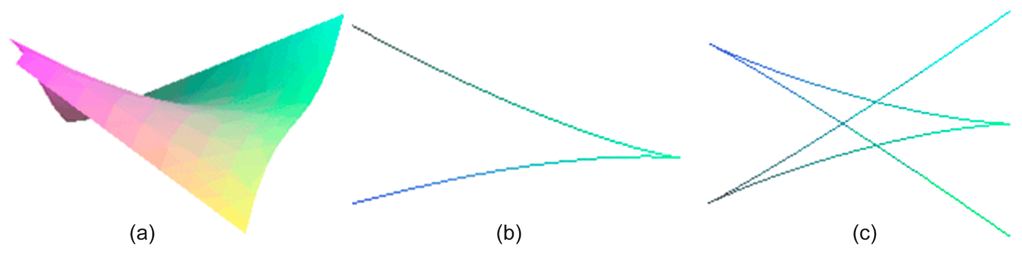
Although the implementation of high-order singularities is an “exceptional state” of the system (it corresponds to an exceptional set of characteristic control parameters), they give a complete (global) picture of the stability change (determine the scenario of the stability change of the entire set of steady states).

The task of implementing a numerical–analytical method of continuation in two parameters (it is necessary to take into account an avalanche increase in the amount of computation as the number of degrees of freedom or the number of input-controllable parameters increases) is of independent interest (Holodniok et al., 1991; Khibnik et al., 1993), and this method has no alternative when describing the model in more detail.

6 Conclusions

The paper presents the successive stages of implementation of the proposed bifurcation approach in the qualitative global analysis of the conditions of divergent stability loss of nonlinear dynamic systems. It is shown that divergent loss of stability of a steady state (the critical case of a single Lyapunov zero root) is associated with the realization of a multiple stationary regime: in the simplest case of change of the stability of a symmetric solution, a three-fold regime is realized. From the origin, either a pair of stable steady states is born, or a pair of unstable steady comes to the origin and merges with a stable steady state. A formal algebraic approach to the analysis of conditions of dangerous–safe divergent stability loss of the stationary regime is illustrated in a model of a wheeled vehicle; it is shown that the change of the nature of dangerous–safe loss of the stability of the rectilinear motion mode of a vehicle model is linked to the realization of a higher rank butterfly bifurcation. For the bifurcation analysis in the case of additional degeneracy of $\mathit{\gamma }\left(v^{+}\right)=\mathrm{0}$, it will be needed to consider the decomposition of the right parts of a dynamic system in Taylor series up to the terms of the fifth order of smallness.