the Creative Commons Attribution 4.0 License.
the Creative Commons Attribution 4.0 License.
 | 18 Mar 2022
Motion generation of a planar 3R serial chain based on conformal geometric algebra with applications to planar linkages
Lei Wang
Gaohong Yu
Liang Sun
Yuzhu Zhou
Chuanyu Wu
A planar three-revolute (3R) serial chain is an important part of many mechanisms. The classical approach in motion generation of a planar 3R serial chain is to construct closed-loop equations based on complex numbers, which yields a large-scale polynomial system. In this study, a new approach of planar 3R serial chain motion generation by establishing the relative kinematics model based on conformal geometric algebra (CGA) is proposed. The simpler design equations are obtained, which can be used to design a planar 3R serial chain that can accurately achieve the N poses. In the numerical examples, the number of different poses is used to verify the correctness and efficiency of the proposed method by using polyhedral homotopy continuation. The results indicate that the design equations obtained via CGA are more concise for improving the solving efficiency compared with the previous method. Finally, a geared five-bar mechanism with a seven-pose motion generation example is considered.
- Article
(1111 KB) - Full-text XML
- BibTeX
- EndNote


Dimensional synthesis is the process of designing link dimensions for a given task or set of tasks (Bottema et al., 1979; Hunt, 1978; Hartenberg and Danavit, 1964). The motion generation task ensures that the design of the mechanism can reach a set of poses comprising positions and orientations (Husty et al., 2007). Burmester (1888) first solved the dimensional synthesis of planar mechanisms for motion generation by using graphic methods, and Freudenstein (1954) subsequently transformed the geometric methods into analytical equations and started the use of computers to generate solutions. McCarthy and Soh (2011) introduced the methods of perpendicular bisector constraint and dyad triangle for planar mechanism dimensional synthesis. Zhao et al. (2016) and Ge et al. (2013) explored the use of kinematic mapping in dimensional synthesis. Han and Qian (2009), Bai et al. (2016) and Glabe and McCarthy (2019) also investigated the synthesis of planar mechanisms. However, these studies only focused on the motion generation of planar four-bar linkages. Generally, the dimensional synthesis of a planar two-revolute (2R) serial chain is the first step in designing four-bar mechanisms. In addition, a planar 2R serial chain can be accurately synthesized with up to five poses in motion generation. When the mechanism needs to reach more than five poses, the planar 2R serial chain fails to reach the end effector precisely at the given design positions.
A planar three-revolute (3R) serial chain can accurately reach any given pose in the working space because it has three degrees of freedom and satisfactory flexibility. This serial chain forms part of many single- and multi-loop mechanisms, such as the six-bar, eight-bar and planar parallel mechanisms (Zhao et al., 2020; Soh and McCarthy, 2008). Dimensional synthesis of a planar 3R serial chain for motion generation is an important process in many mechanisms' design. Wampler and Sommese (2011) systematically introduced forward and inverse kinematic analysis and planar 3R serial chain synthesis. Chase et al. (1987) performed planar 3R serial chain synthesis for five prescribed positions and applied it to the design of planar six-bar linkages. Subbian and Flugrad (1993) also investigated the five-position synthesis of a planar 3R serial chain and used it to design a four-bar function-generating mechanism and a six-bar linkage. Lin and Erdman (1987) applied the compatibility linkage approach to obtain the Burmester curves of a planar 3R serial chain for a six-position synthesis problem. Using a continuation method, Subbian and Flugrad (1994) accomplished six- and seven-position syntheses of a planar 3R serial chain for motion generation with prescribed timing. Perez and McCarthy (2005) derived design equations from the relative kinematic equations of the chain to design nR planar serial chains.
However, the above-mentioned studies were all on the basis of standard form equations (Erdman and Sandor, 1997), which created loop equations for a given chain from a reference position of the end effector to a desired position. The design equations established by this method contain numerous sine and cosine trigonometric functions. To solve these equations, the trigonometric functions are replaced by the introduction of new variables or eliminated using half-tangent substitutions, which unavoidably increases the scale of polynomial equations. Therefore, it is important to find a simpler mathematical model in the mechanism design process.
Conformal geometric algebra (CGA) is a new mathematical language and calculation tool with remarkable advantages in geometric modeling and calculation (Hildenbrand, 2012; Li, 2005) which is widely used in physics, computer vision, computer graphics and robotics (Perwass, 2009). Hildenbrand et al. (2008) used CGA to analyze the inverse kinematic solution of a robot. Kim et al. (2015) applied CGA to solve inverse kinematics and analyze the singularity of the mechanism of 3-SPS/S redundant motion. Zhu et al. (2022) and Zhang (2018) analyzed the forward kinematic modeling of the 3-RPR planar parallel mechanism based on CGA. Fu et al. (2013) proposed an effective method to solve the inverse kinematics problem of a 6R offset wrist robot based on geometric algebra. Hrdina et al. (2016) solved the local controllability of a three-link robotic snake with CGA and assembled the forward, differential and non-holonomic kinematic equations of the robot. Therefore, CGA can be applied to the dimensional synthesis of the mechanisms to obtain a simpler and more intuitive kinematic model.
In this study, a new method for constructing the kinematic synthesis model of a planar 3R serial chain based on CGA is proposed. The simpler design equations are obtained by the relative kinematics model of the chain, established by the rotor in CGA and solved using polyhedral homotopy continuation. The proposed method simplifies the formulation to solve the equations clearly and efficiently.
The rest of this paper is organized as follows: the concept of CGA is introduced in Sect. 2. In Sect. 3, the kinematic equations of the planar 3R serial chain are established using rotors in CGA. The motion synthesis of different numbers of precise poses of the planar 3R serial chain is discussed, and some numerical examples are solved in Sect. 4. In Sect. 5, the proposed method is applied to design a single degree-of-freedom (DOF) geared five-bar mechanism. Lastly, the results are discussed, and the conclusions are presented in Sect. 6.
In this section, a brief overview of CGA is presented, and its basic elements and transformations are discussed in a geometrically intuitive manner. More details about CGA can be found in Hildenbrand (2012), Vince (2008) and Wareham et al. (2004).
2.1 Basic elements
The fundamental algebraic operator in geometric algebra is the geometric product, which can be expressed as
where “⋅” and “∧” denote the inner and outer products, respectively, which can be derived from Eq. (1):
The inner product of two vectors is the same as the well-known Euclidean scalar product of two vectors. The outer product of the two vectors u and v represents a directed parallelogram that u sweeps along v. For vectors u, v, and w, represents a three-dimensional solid with a direction.
In geometric algebra, the basic elements are blades. An n-dimensional geometric algebra consists of blades with grades varying from 0 to n, where a scalar is a 0-blade (a blade of grade 0) and the 1-blades are the basis vectors e1, e2, …, en. The element with the highest grade n, , is called the pseudo-scalar. The linear combination of k blades is called k-vector, and the linear combination of blades with different grades is called multi-vector. CGA is a type of 5D geometric algebra that uses the three Euclidean basis vectors e1, e2, e3 and two additional basis vectors e+, e− with the properties of
Therefore, the two null vectors can be defined as , which represents the 3D origin, and , which represents infinity.
These new basis vectors have the following properties:
As such, the five vector bases for CGA are .
The duality of the multi-vector A is defined as
where is the pseudo-scalar in CGA.
2.2 Basic geometric entities
In CGA, many basic geometric bodies, such as points, spheres, planes, circles, lines and point pairs, can be expressed indirectly and intuitively. These entities have two algebraic representations: the inner-product null space (IPNS) and the outer-product null space (OPNS). The IPNS and OPNS describe the null spaces of algebraic expressions with respect to the inner and outer products, respectively. These representations are dual to each other (Hildenbrand, 2012). This section only introduces the representation of points and lines related to this study.
The point x of the three-dimensional Euclidean space can be expressed in CGA as
where and . Note that the previous object is expressed in the IPNS representation.
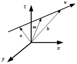
Starting from the representation of a point in CGA, the representation of several Euclidean geometric objects can be generated with the outer product in the OPNS representation. The two points A and B on a line are presented in the Euclidean space, as shown in Fig. 1. The line can be represented in CGA by
where PA and PB are the conformal representations of two points on the line and LO denotes the OPNS representation of the line.
Equation (9) shows that a line in the space can be constructed by using the outer product between two points that lie on it and the point at infinity. In addition, the line can also be represented by the six Plücker coordinates in the IPNS representation. In Fig. 1, A and B are two different points on the line, and their position vectors are a and b, respectively. The Plücker coordinates of the line can be identified in CGA as
or
where and represent the line orientation and moment, respectively. Equation (11) is the IPNS representation of the line.
2.3 Transformations and motions
Rigid transformations, including rotation and translation, can easily be described in CGA.
The rotation can be computed as a rotor
where L is an arbitrary line representing the axis of rotation in the IPNS representation and θ is the rotation angle around this axis.
The translation can be represented as a translator
where is a vector representing the direction and length of a translation.
Therefore, a rigid body motion, including a rotation and a translation, is described by the following displacement motor in CGA:
A rigid body motion of an object o is described as follows:
where and .
In CGA, the rotation and translation can be expressed in one algebraic expression. The advantage of rigid transformation representation in CGA is the simplification of the composition of groups into geometric products (Bayro-Corrochano, 2019).
3.1 Planar displacement
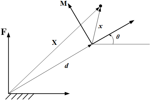
Let M be a coordinate frame attached to the moving body and F be a fixed reference frame. The moving frame is rotated by the angle θ and measured positive anti-clockwise relative to F. The origin of M is located relative to F with a displacement vector d, as shown in Fig. 2. Thus, the displacement that defines the position of the moving frame M relative to the fixed frame F is the following coordinate transformation:
or
In addition, CGA provides a convenient way to describe planar rigid body displacements as follows:
where
and is the inverse of D.
3.2 Pole of relative displacement
A single point that does not move exists in the general planar displacement. This point is called the pole of the displacement (see Fig. 3). A general planar displacement can be viewed as a pure rotation around this pole. The two poses Mi and Mj of a rigid body are considered and defined by using the displacements [Ti] and [Tj] relative to F. The transformation [Tij] is defined by
This equation explains the relative displacement from Mi to Mj measured in F.

The pole is unchanged by the planar displacement . According to Eq. (19),
The coordinates of Pij can be determined as
where
Equation (20) can be used to define the translation component of the displacement in terms of the coordinates of the pole. Thus, the planar displacement can be defined directly in terms of the rotation angle θij and pole Pij as follows:
Thus,
Moreover, in CGA, Eq. (22) can be defined as
where R(θij) represents the rotor that rotates θij around the point Pij.
3.3 Kinematic equations for the planar 3R serial chain of CGA
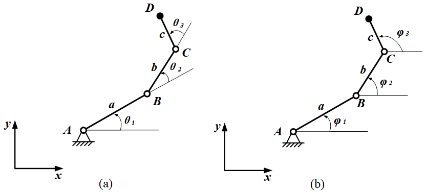
A kinematic chain connected by 3R joints with parallel axes is called a planar 3R serial chain (see Fig. 4). The relative rotation angles in Fig. 4a, the absolute rotation angles in Fig. 4b and the link lengths are denoted as θ1, θ2, θ3, φ1, φ2, φ3 and a1, a2, a3, respectively.
Then, the kinematic equation of the planar 3R chain is presented as
where
and [X(ai)] defines the translation ai distance along the x axis. The transformation [G] defines the position of the base A relative to the world frame. Therefore, the matrix [D] defines the position of the end effector of the planar 3R serial chain as follows:
where and .
The product of the transformation matrices defines the kinematic equation of the planar 3R serial chain. In the same way, CGA provides an elegant and compact method for describing the kinematics of the planar 3R serial chain. Although the classical approach is based on transformation matrices, the proposed approach only needs the elements of the motor group.
The rotors and translators can be defined as follows:
and the motors are defined as
Therefore, Eq. (24) can be determined in CGA as follows:
This equation represents the position of the end effector via the transition point, and the transition line indicates the orientation of the end effector. Given the values of the joint angles, the forward kinematic problem is the computation of the position and orientation of the end effector. The converse of the forward kinematic problem is the inverse kinematic problem, which determines the joint angles that place the end effector in the desired position and orientation.
The purpose of the design problem in this study is to determine the dimensions of the planar 3R serial chain, which can enable the end effector to reach a given set of task poses. The locations of the base, the link dimensions, and the joint angles are considered design variables.
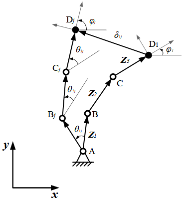
A planar 3R serial chain in two finitely separated positions is shown in Fig. 5. The initial position can be expressed by the position vectors Z1, Z2, and Z3. These vectors represent the three binary links, which are denoted by the positions of joints A, B, C, and D. After the mechanism moves to another position (jth position), the joint positions are expressed as A, Bj, Cj, and Dj. The displacement equation of the planar 3R serial chain can then be obtained from the vector loop closure of the pivots of A–B–C–D–Dj–Cj–Bj–A:
where θ1j, θ2j, and θ3j denote the angular displacements of the three links from their initial positions, and δ1j is the end-point displacement of the planar 3R serial chain. Erdman and Sandor (1997) called Eq. (29) the standard form equation.
In this study, a new modeling method based on CGA to obtain the design equations of a planar 3R serial chain is proposed. According to Sect. 3.2, the relative displacement from one location to another is equivalent to a pure rotation around the pole. Similarly, the two given poses D1 and Dj at the end of the planar 3R serial chain are shown in Fig. 5. In accordance with Sect. 3.2, the movement from position D1 to position Dj can be regarded as the rotation φ1j around the pole P1j to obtain the following:
Furthermore, the end effector can also move from position D1 to position Dj by rotating θ3j, θ2j, and θ1j around hinge points C, B, and A, respectively.
According to Eqs. (30) and (31), it is easy to obtain
The above equation only contains four rotation relationships around the fixed point. In CGA, this relationship can be expressed as the geometric product between the rotors.
Firstly, a point in the plane can be obtained from the Plücker coordinates in CGA as the z axis that passes through that point as , where represents the direction of the z axis and denotes the moment of this axis to the origin.
Then, a point in the plane can be expressed in the CGA as the axis passing through that point in space, as follows:
The three revolution joints of the planar 3R serial chain and the pole can be expressed as
Furthermore, the rotation around these points can be expressed as
Hence, Eq. (32) can be expressed in CGA as follows:
where
By using the inverse of the rotor, Eq. (35) can be converted into
and then expanding the left- and right-hand sides of the above equation as follows:
and
where
The coefficients of the scalar and vector parts of the expanded equation should be equal. By extracting and subtracting the coefficients of the left- and right-hand sides, respectively, it is found that the scalar part and e12 are eliminated. Furthermore, the coefficients of e1∞ and e2∞ are subtracted to obtain the following design equations:
To simplify this equation, dividing the above two expressions by A1j gives
where
Equation (40) can be applied to design the planar 3R serial chains. It is noteworthy that there are no cosine and sine trigonometric functions, and no variable substitution is required in the solving, which greatly reduces the scale of the polynomial system, thereby greatly improving the efficiency of the design mechanism.
4.1 Number of design poses and free parameters
The planar 3R serial chain has three degrees of freedom and can reach any set of positions within its workspace boundary. However, the number of equations increases with the number of designated positions. Using Eq. (40) to synthesize the planar 3R serial chain for N poses motion generation, and the unknowns mainly include the six coordinate parameters of the three revolution joints xA, yA, xB, yB, xC, yC and the relative angles θ1j, θ2j, , that increase with the positions. Table 1 presents the relationship between the number of equations and unknowns when Eq. (40) is used to synthesize the planar 3R serial chain.
Table 1Number of equations and number of unknowns of the planar 3R serial chain.

Table 1 demonstrates that the number of unknowns is always greater by six numbers compared with the number of equations in any given position. This feature shows that regardless of how many positions there are in the synthesis of the planar 3R serial chain, six parameters should be provided. This finding is consistent with that of the Perez and McCarthy (2005) theory. The six given parameters for the synthesis of the planar 3R serial chain also indicate that the number of synthesis mechanisms is infinite. Hence, designing and optimizing the mechanism to achieve our purpose becomes more convenient. In this section, Eq. (40) is used to discuss the synthesis problem of the planar 3R serial chain for N precision positions.
4.2 Numerical examples and discussion
In this section, a planar 3R serial chain is designed to ensure that it guides a rigid body through some precision poses. These poses are defined by two elements, namely the position coordinates of the origin of the end-effector frame with respect to the fixed reference frame and the direction of the end-effector frame with respect to the fixed reference frame. The basic steps for motion synthesis of a planar 3R serial chain reaching any N poses are as follows.
-
Giving N planar poses
-
Selecting the first pose as the reference and computing the relative displacement from the reference pose to the other poses based on Eq. (19)
-
Using Eq. (20) to find the poles P1j and the end-effector relative angles
-
Constructing Eq. (40) by using rotors in CGA
-
Substituting P1j, φ1j, and six specified parameters into Eq. (40) yields two (N−1) design equations.
-
Solving the design equations
Based on this method, the design equations established by CGA are used to carry out the motion synthesis of the number of different poses to be accurately realized by the planar 3R serial chain. The design equations are obtained by using the CLIFFORD package (Ablamowicz and Fauser, 2005) in the MAPLE 2017 software. All the computations were performed using the HOM4PS-2.0 package (Lee et al., 2008) in the MATLAB R2014a software, which runs on a 3.2 GHz Intel (R) Core (TM) i7-8700 CPU with 64-bit Windows and 8 GB memory. The numerical results are shown in Table 2. The second column in the table is the data sources for these poses. By specifying six different parameters, the number of solutions, the number of real solutions, and the time spent by the CPU are obtained for each group of data, respectively, and the path tracked by using HOM4PS-2.0 is counted.
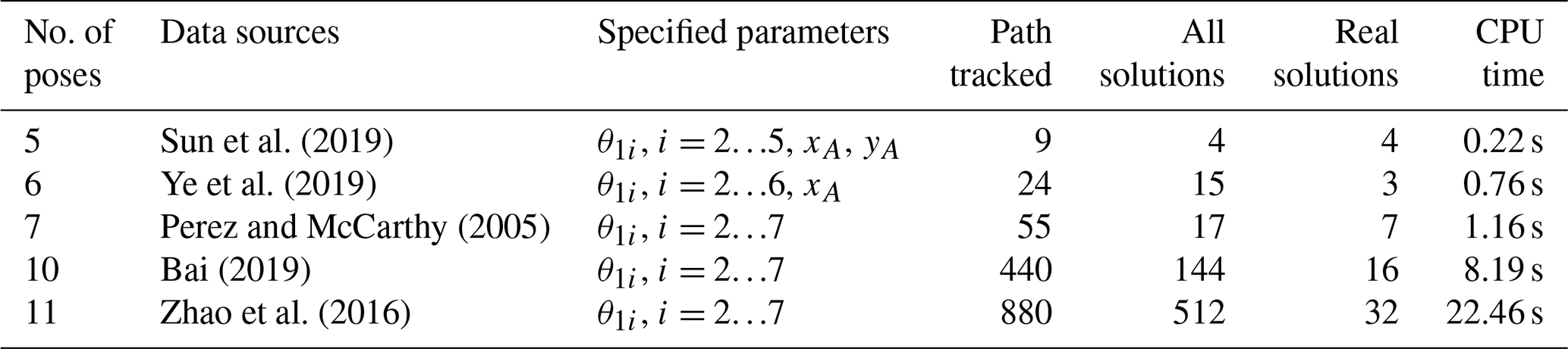
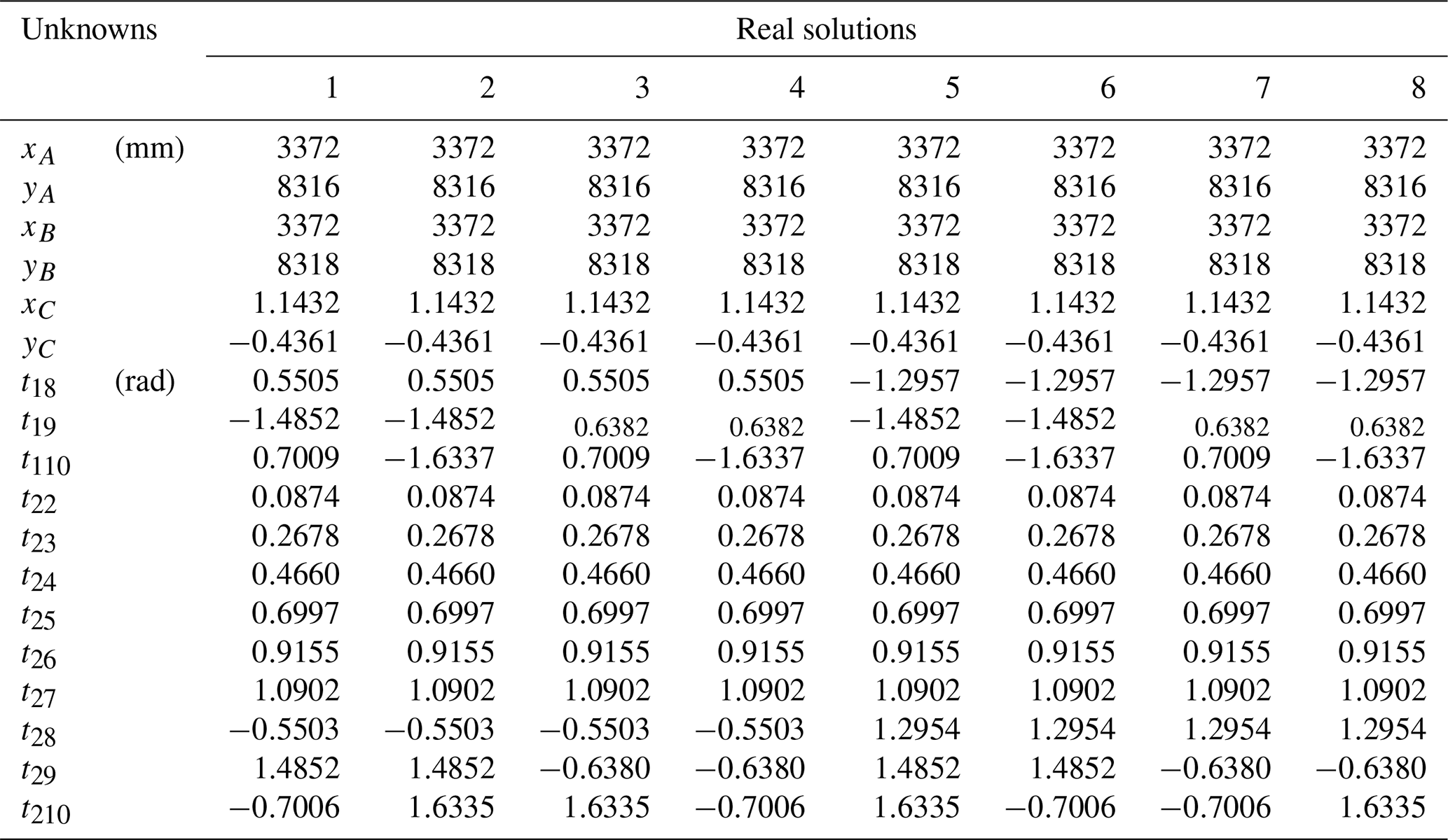
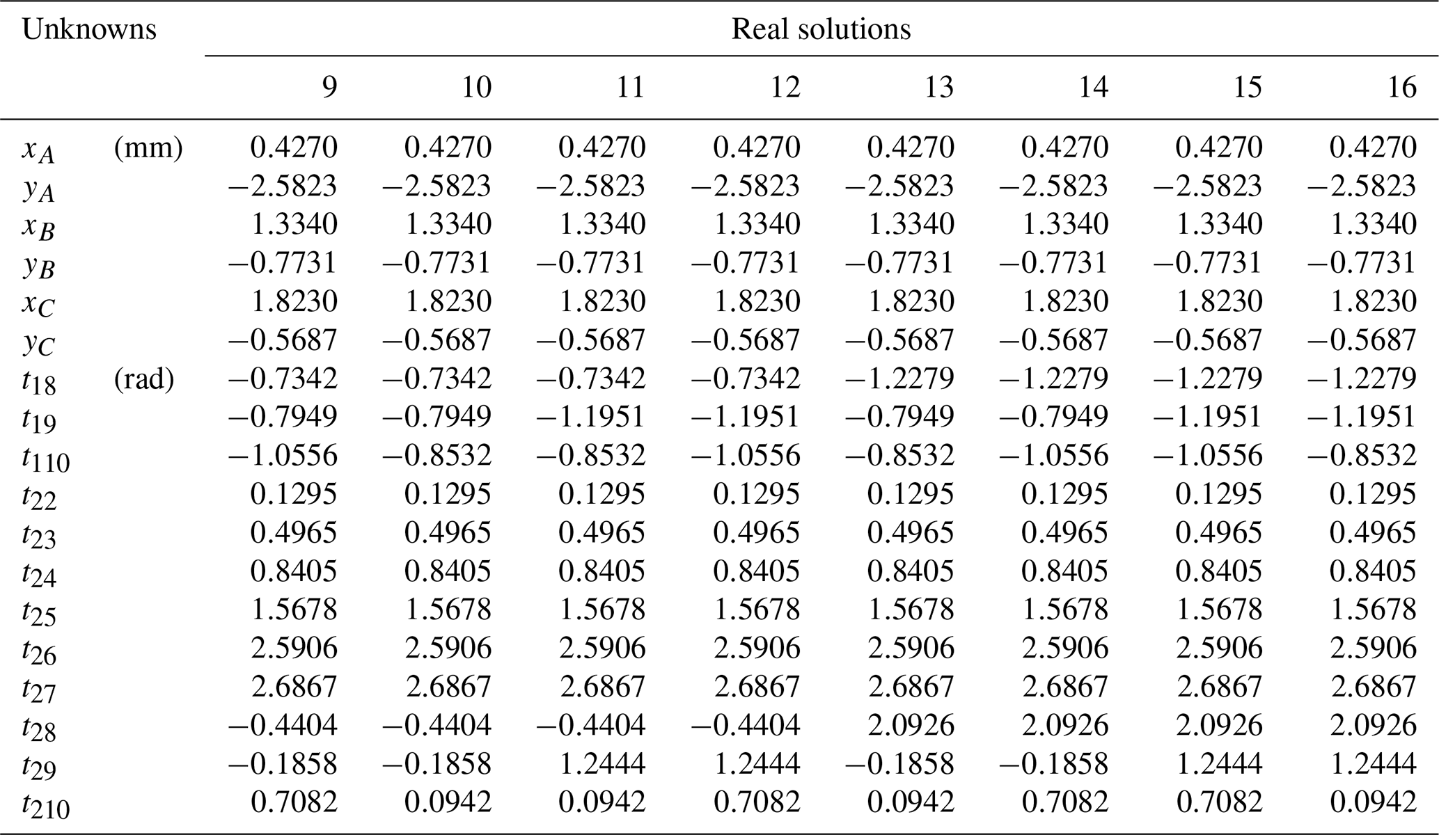
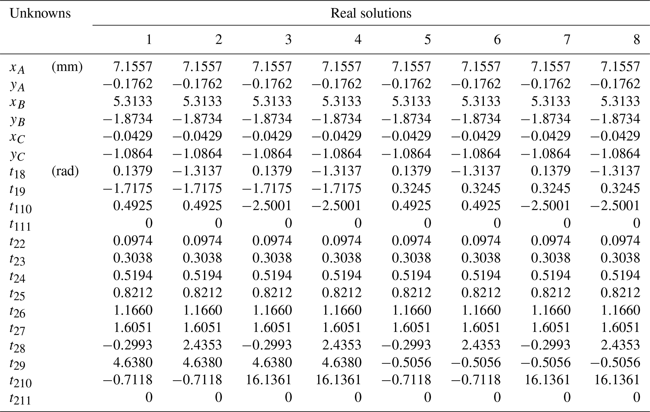
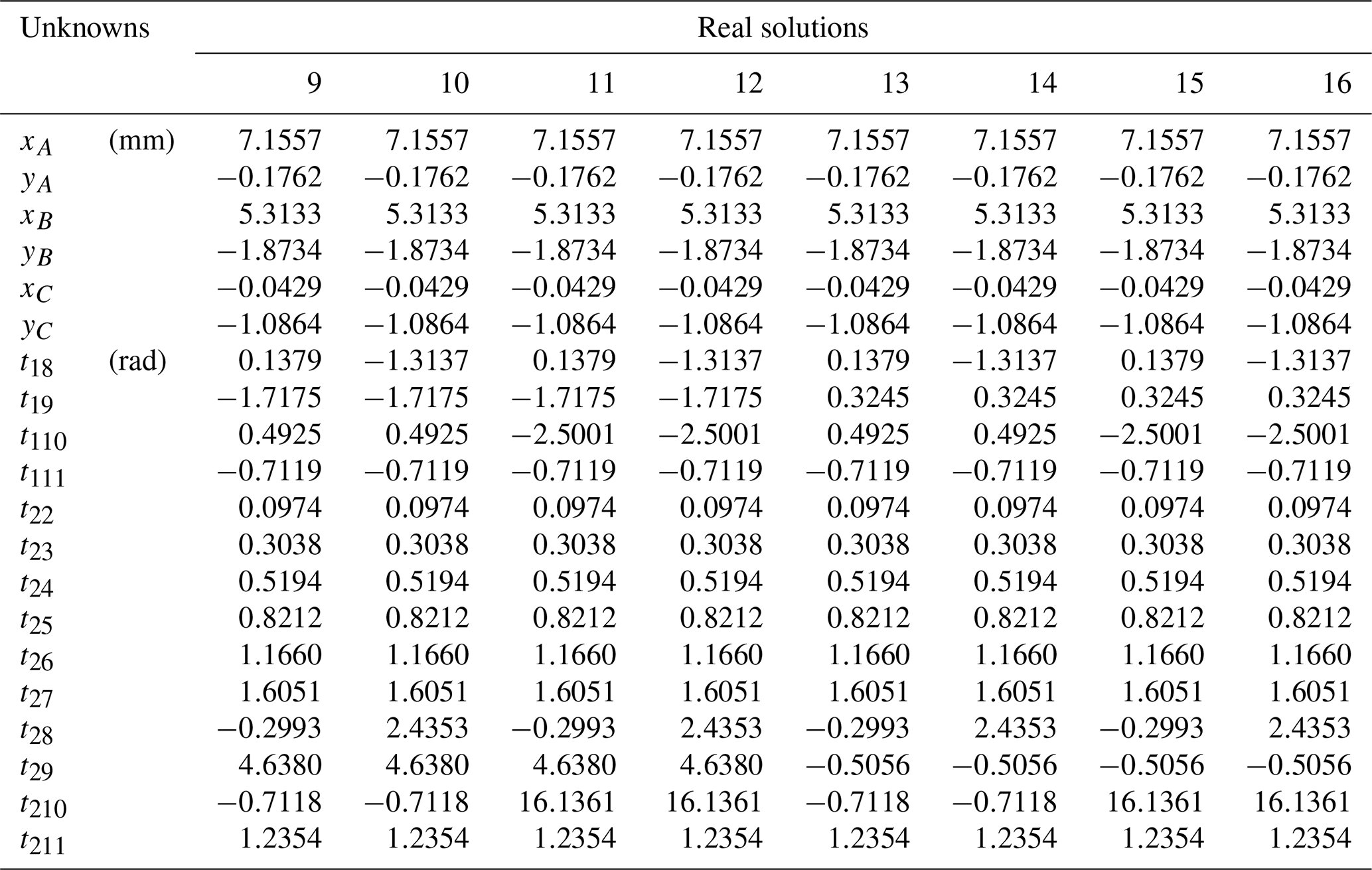
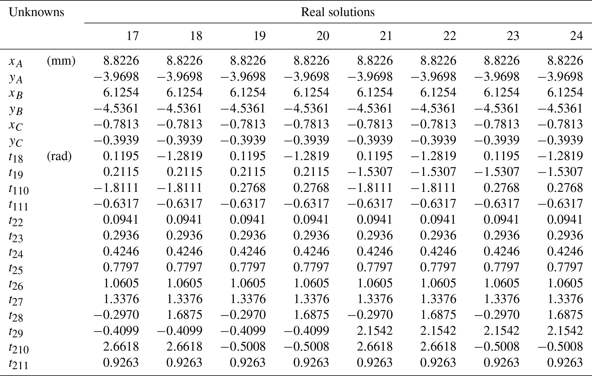
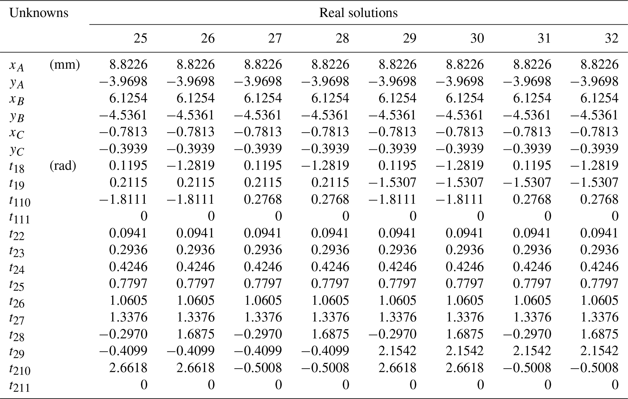
As shown in the table, with the increase in the number of poses, the number of solutions obtained also increases, which indicates that the given six parameters impose more constraints on the mechanism in the case of the synthesis of fewer poses, while the six parameters impose fewer constraints on the mechanism in the case of the increase in poses. So, more solutions can be obtained and more candidate mechanisms can be selected. It should be noted that there are only two sets of physical solutions (Tables A4–A9 in the Appendix) in the real number solutions given of 10 and 11 poses, and the other real number solutions are different combinations of motion parameters. This is because more poses add more constraints to the problem, but its motion form is flexible. At the same time, the computing time used by the CPU is also increasing, because the scale of the polynomial system is also increasing. In addition, all the real solutions of different poses listed in the Appendix are verified, and all the results are correct.
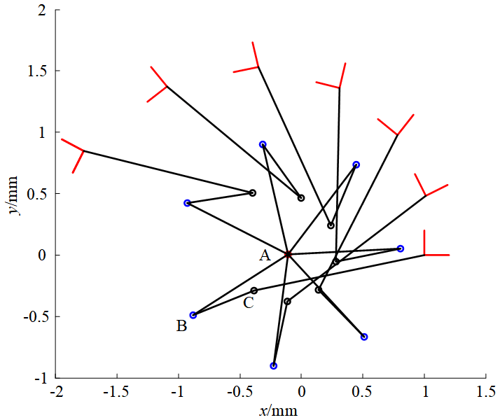
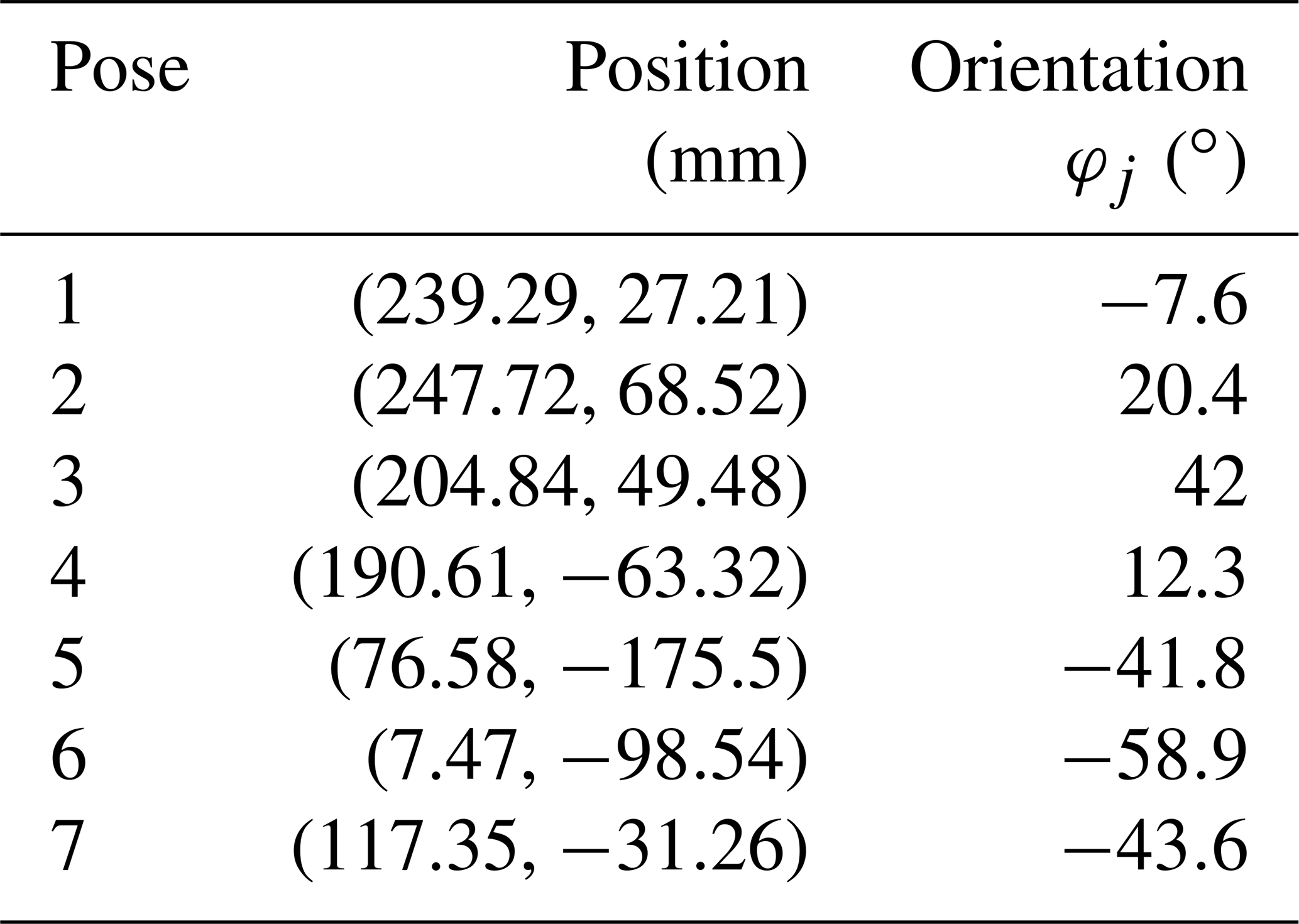
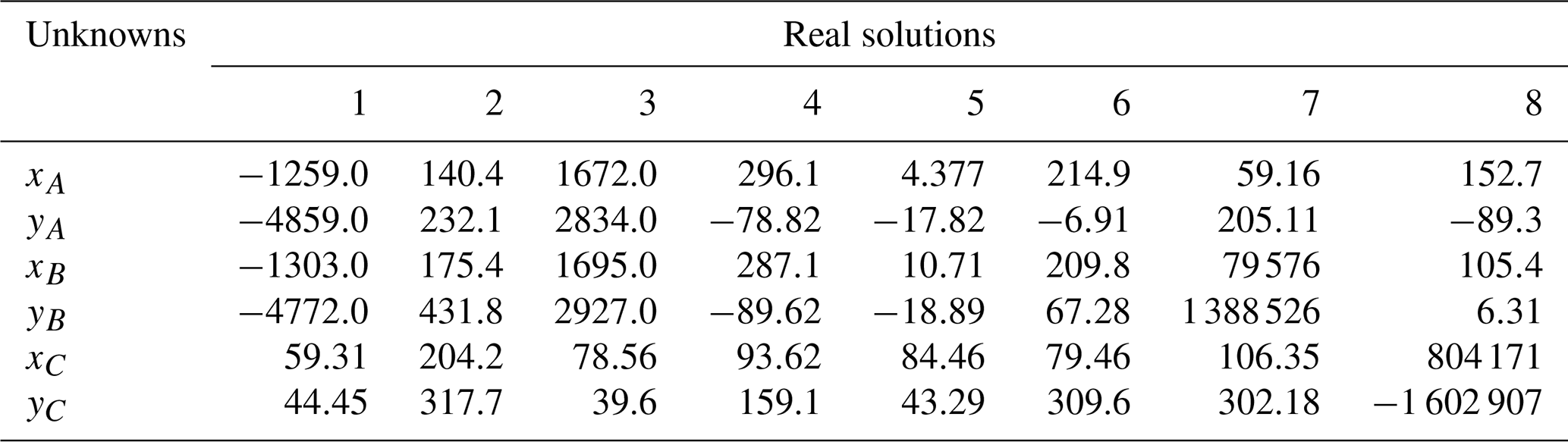
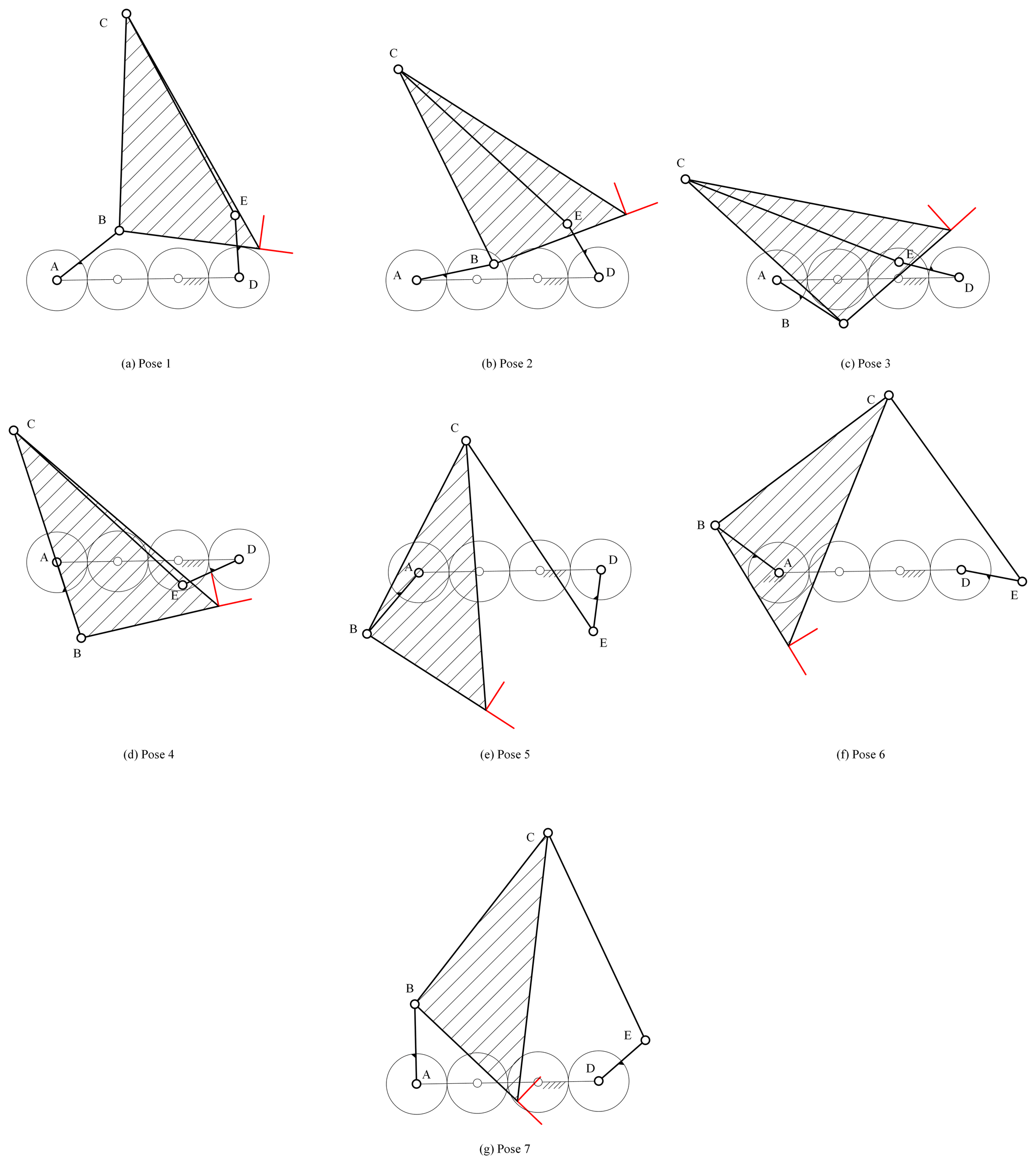
As a concrete example, a planar 3R serial chain was designed to enable its end effector to accurately reach seven specified poses and was compared with the previous method. The seven precision poses and prescribed values for θ1j are the same as in the reference (Perez and McCarthy, 2005). Substituting the specified parameters in Table 3 into Eq. (40), the result is 12 equations with 12 unknowns of a planar 3R serial chain. The HOM4PS-2.0 software package was used to solve these equations, and 55 paths were tracked in approximately 1.16 s and 17 paths converge to the solutions, of which only 7 were real solutions. The real solutions are listed in Table A3. Figure 6 shows that the design of a planar 3R serial chain reaches the seven poses corresponding to solution 1.
As a comparison, Eq. (29) is used to construct the design equations, and 12 equations are obtained. However, these equations are complicated and contain a huge number of sine and cosine functions. In order to solve these equations, we replaced them and introduced constraint equations , . Therefore, 18 equations with 18 unknowns must be solved. Similarly, the HOM4PS-2.0 software package was used to solve these equations on the same computer. In this case, the tracking path was 78 016, which took 20.4 min to compute, and the same 17 sets of solutions were obtained. The comparison results show that the method presented in this paper is correct, and the design equations obtained via CGA are simpler and faster to solve compared with the previous closed-loop equations.
Many linkage mechanisms can be broken into components consisting of planar 2R and 3R serial chains, such as the five-bar and six-bar mechanisms. In this section, an application example will be used to demonstrate the application of dimensional synthesis of a planar 3R serial chain in linkage mechanism synthesis. Figure 7 shows an equal-speed ratio single-DOF geared five-bar mechanism, which can be designed by simplifying it to a combination of planar 2R serial chain EDP and planar 3R serial chain ABCP.
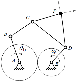
It is assumed that a 2-DOF planar 2R serial chain mechanism EDP can realize the seven positions in Table 3, and the coordinate parameters of its rotation centers E and D are mm, mm, xD1=72.2 mm, and yD1=49.8 mm. It is required to design a 1-DOF geared five-bar mechanism that can make its end points pass through the seven positions given in Table 3 in sequence.
According to the coordinate parameters of the planar 2R open-chain mechanism EDP, the relative angular displacement data of the link ED when the open-chain mechanism EDP reaches seven poses are obtained through the inverse kinematics solution: these are . Set the gear transmission ratio to −1 and calculate the angular displacement data of the AB link in the open-chain 3R mechanism ABCP from the first position to the other positions . By substituting the pose data and θ1i in Eq. (40), HOM4PS-2.0 was used to obtain 20 solutions, among which only 8 solutions in Table 4 were real. Each planar 3R serial chain in Table 4 could be combined with planar 2R mechanism ED to obtain a geared five-bar mechanism that could pass the seven poses specified in Table 4.
Considering the compactness of the mechanism, solutions 1, 4, 7, and 8 in Table 4 were first excluded because of their large size. After confirming that there is a crank and that the mechanism has no defect, the sixth solution in Table 4 was selected as the open-chain 3R mechanism ABCP and combined with the given open-chain 2R mechanism ED to form a five-bar mechanism. Figure 8 shows the state diagram of the finally designed five-bar mechanism when it reaches the seven given poses in Table 3. Coupling the gear with the transmission ratio of −1 between the cranks AB and ED of the five-bar mechanism can restrict the five-bar mechanism to a single DOF gear five-bar mechanism. The mechanism has a stable and continuous motion and reasonable design, which further verifies the correctness and feasibility of the proposed method.
In this study, a new method for the dimensional synthesis of the planar 3R serial chain for motion generation based on CGA is presented. The kinematic equations of the relative displacement of the planar 3R serial chain were established on the basis of the motion transformation operators in CGA. This method greatly reduces the scale of the polynomial system.
In the numerical examples, the motion synthesis of the number of different poses to be accurately realized by the planar 3R serial chain was verified via this method. When the same problem is solved by the same software on the same computer, the computational efficiency of the CGA method has obvious advantages.
Finally, an application example is given to illustrate the application of dimensional synthesis of a planar 3R serial chain in the design of a geared five-bar mechanism. The proposed method provides a new meaning for the motion synthesis of planar serial chains and can be applied to many other types of planar mechanisms. Furthermore, the application of CGA is extended to the mechanism and theoretical method of kinematics synthesis.
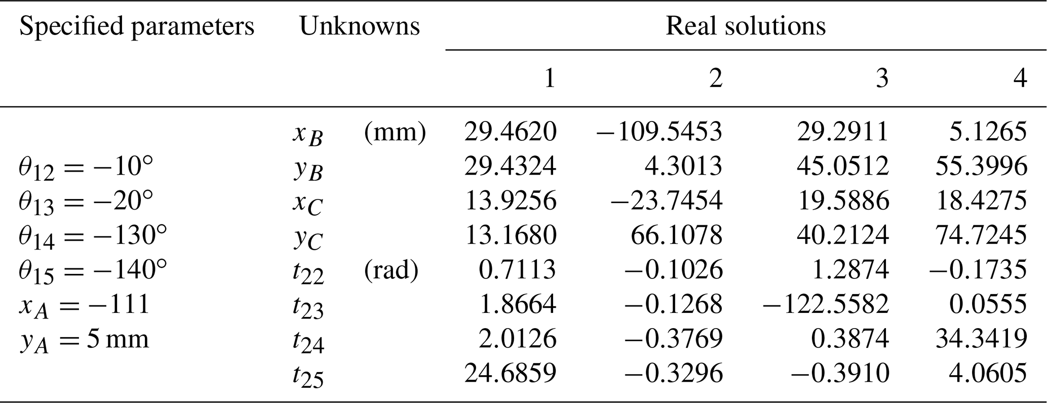
A1 Five poses
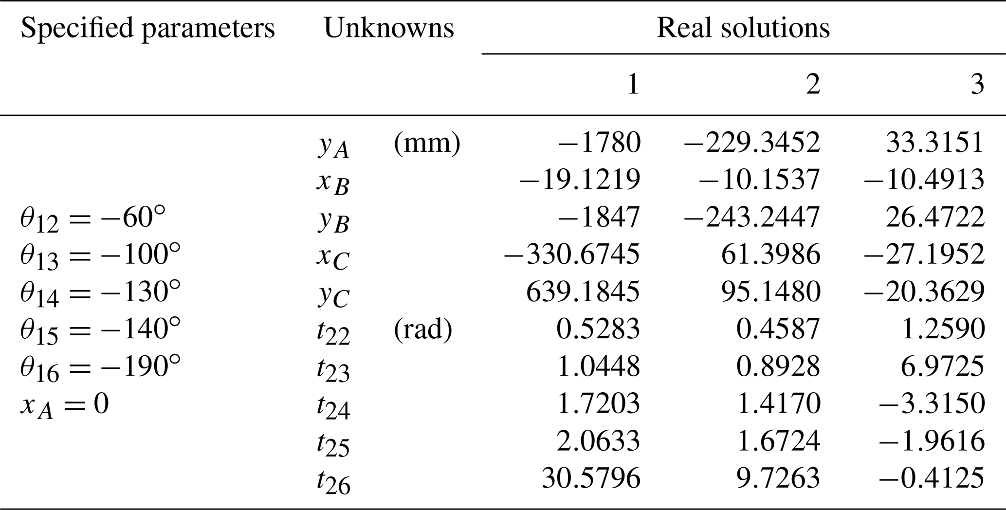
A2 Six poses
A3 Seven poses

A4 Ten poses
Specified parameters: ∘, ∘, ∘, ∘, ∘, ∘.
A5 Eleven poses
Specified parameters: ∘, ∘, ∘, ∘, ∘, ∘.
Code and data can be made available upon request.
Conceptualization, methodology, writing and original draft preparation were done by LW. Data curation, writing, review and editing, software, visualization, and validation were handled by YZ. Supervision and project administration were done by LS, GY and CW. All the authors have read and agreed to the published version of the paper.
The contact author has declared that neither they nor their co-authors have any competing interests.
Publisher’s note: Copernicus Publications remains neutral with regard to jurisdictional claims in published maps and institutional affiliations.
This work was supported in part by the National Natural Science Foundation of China (grant nos. 51975534 and 52075497), in part by the Zhejiang Provincial Key Research and Development Program (grant no. 2022C02006), in part by the 151 Talent Plan of Zhejiang Province, and in part by the Project of Zhejiang Provincial Young and Middle-aged Discipline Leaders.
This paper was edited by Daniel Condurache and reviewed by two anonymous referees.
Ablamowicz, R. and Fauser, B.: Mathematics of Clifford – a Maple package for Clifford and Grassmann algebras, Adv. Appl. Clifford Al., 15, 157–181, https://doi.org/10.1007/s00006-005-0009-9, 2005.
Bai, S.: Exact Synthesis of a 1-dof Planar Linkage for Visiting 10 Poses, IFToMM World Congress on Mechanism and Machine Science, https://doi.org/10.1007/978-3-030-20131-9_127, 2019.
Bai, S., Wang, D., and Dong, H.: A Unified Formulation for Dimensional Synthesis of Stephenson Linkages, J. Mech. Robot., 8, 041009, https://doi.org/10.1115/1.4032701, 2016.
Bayro-Corrochano, E.: Kinematics of the 2D and 3D Spaces, in: Geometric Algebra Applications Vol. I, Springer, Cham, 209–231, https://doi.org/10.1007/978-3-319-74830-6_7, 2019.
Bottema, D., Roth, B., and Veldkamp, G. R.: Theoretical Kinematics, North-Holland, Amsterdam, https://doi.org/10.1016/0094-114X(83)90112-X, 1979.
Burmester, L.: Lehrbuch der Kinematik, Verlag Von Arthur Felix, Leipzig, Germany, 1888.
Chase, T. R., Erdman, A. G., and Riley, D. R.: Triad Synthesis for up to Five Design Positions With Application to the Design of Arbitrary Planar Mechanisms, J. Mech. Design, 109, 426–434, 1987.
Erdman, A. G. and Sandor, S. G. N.: Mechanism design: analysis and synthesis, Vol. 1, Prentice-Hall, Inc., https://doi.org/10.1016/0094-114X(85)90061-8, 1997.
Freudenstein, F.: An analytical approach to the design of four-link mechanisms, T. ASME, 76, 483–492, 1954.
Fu, Z., Yang, W., and Zhen, Y.: Solution of Inverse Kinematics for 6R Robot Manipulators With Offset Wrist Based on Geometric Algebra, J. Mech. Robot., 5, 310081–310087, 2013.
Ge, Q. J., Ping, Z., and Purwar, A.: Decomposition of Planar Burmester Problems Using Kinematic Mapping, in: Advances in mechanisms, robotics and design education and research, Springer Heidelberg, 145–157, https://doi.org/10.1007/978-3-319-00398-6_11, 2013.
Glabe, J. and McCarthy, J. M.: Five Position Synthesis of a Planar Four-Bar Linkage, IFToMM World Congress on Mechanism and Machine Science, https://doi.org/10.1007/978-3-030-20131-9_60, 2019.
Han, J. and Qian, W.: On the solution of region-based planar four-bar motion generation, Mech. Mach. Theory, 44, 457–465, 2009.
Hartenberg, R. and Danavit, J.: Kinematic synthesis of linkages, McGraw-Hill, New York, 1964.
Hildenbrand, D.: Foundations of Geometric Algebra computing, Springer Science & Business Media, https://doi.org/10.1063/1.4756054, 2012.
Hildenbrand, D., Zamora, J., and Bayro-Corrochano, E.: Inverse Kinematics Computation in Computer Graphics and Robotics Using Conformal Geometric Algebra, Adv. Appl. Clifford Al., 18, 699–713, 2008.
Hrdina, J., Návrat, A., and Vašík, P.: Control of 3-Link Robotic Snake Based on Conformal Geometric Algebra, Adv. Appl. Clifford Al., 26, 1069–1080, 2016.
Hunt, K. H.: Kinematic geometry of mechanisms, Oxford University Press, New York, https://doi.org/10.1137/1033163, 1978.
Husty, M. L., Pfurner, M., Schrocker, H. P., and Brunnthaler, K.: Algebraic methods in mechanism analysis and synthesis, Robotica, 25, 661–675, https://doi.org/10.1017/S0263574707003530, 2007.
Kim, J. S., Jeong, J. H., and Park, J. H.: Inverse kinematics and geometric singularity analysis of a 3-SPS/S redundant motion mechanism using conformal geometric algebra, Mech. Mach. Theory, 90, 23–36, 2015.
Lee, T. L., Li, T. Y., and Tsai, C. H.: HOM4PS-2.0: a software package for solving polynomial systems by the polyhedral homotopy continuation method, Computing, 83, 109–133, https://doi.org/10.1007/s00607-008-0015-6, 2008.
Li, H.: Conformal geometric algebra – A new framework for computational geometry, Journal of Computer Aided Design & Computer Graphics, 17, 2383–2393, 2005.
Lin, C. S. and Erdman, A. G.: Dimensional synthesis of planar triads: Motion generation with prescribed timing for six precision positions, Mech. Mach. Theory, 22, 411–419, 1987.
McCarthy, J. M. and Soh, G. S.: Geometric Design of Linkages, Springer, New York, https://doi.org/10.1007/978-1-4419-7892-9, 2011.
Perez, A. and McCarthy, J. M.: Clifford Algebra Exponentials and Planar Linkage Synthesis Equations, J. Mech. Design, 127, 931–940, 2005.
Perwass, C.: Geometric Algebra with Applications in Engineering, Springer Berlin Heidelberg, https://doi.org/10.1007/978-3-540-89068-3, 2009.
Soh, G. S. and McCarthy, J. M.: The synthesis of six-bar linkages as constrained planar 3R chains, Mech. Mach. Theory, 43, 160–170, 2008.
Subbian, T. and Flugrad, D. R.: Five Position Triad Synthesis With Applications to Four- and Six-Bar Mechanisms, ASME J. Mech. Des., 115, 262–268, https://doi.org/10.1115/1.2919186, 1993.
Subbian, T. and Flugrad, D. R.: Six and Seven Position Triad Synthesis Using Continuation Methods, J. Mech. Design, 116, 660–665, 1994.
Sun, L., Wang, Z., Wu, C., and Zhang, G.: Novel approach for planetary gear train dimensional synthesis through kinematic mapping, P. I. Mech. Eng. C-J. Mec., 234, 273–288, https://doi.org/10.1177/0954406219832912, 2019.
Vince, J. A.: Geometric algebra for computer graphics, Springer Science & Business Media, https://doi.org/10.1007/978-1-84628-997-2, 2008.
Wampler, C. W. and Sommese, A. J.: Numerical algebraic geometry and algebraic kinematics, Acta Numer., 20, 469–567, 2011.
Wareham, R., Cameron, J., and Lasenby, J.: Applications of Conformal Geometric Algebra in Computer Vision and Graphics, in: Computer algebra and geometric algebra with applications, Springer, Berlin, Heidelberg, 329–349, https://doi.org/10.1007/11499251_24, 2004.
Ye, J., Zhao, X., Wang, Y., Sun, X., and Xia, X.: A novel planar motion generation method based on the synthesis of planetary gear train with noncircular gears, J. Mech. Sci. Technol., 33, 4939–4949, https://doi.org/10.1007/s12206-019-0933-6, 2019.
Zhang, Y.: Geometric Modeling and Free-elimination Computing Method for the Forward Kinematics Analysis of Planar Parallel Manipulators, J. Mech. Eng., 54, 27, https://doi.org/10.3901/JME.2018.19.027, 2018.
Zhao, P., Ge, X., Zi, B., and Ge, Q. J.: Planar Linkage Synthesis for Mixed Exact and Approximated Motion Realization Via Kinematic Mapping, J. Mech. Robot, 8, 051004, https://doi.org/10.1115/1.4032212, 2016.
Zhao, X., Yu, C., Chen, J., Sun, X., and Zhou, Q.: Synthesis and Application of a Single Degree-of-Freedom Six-Bar Linkage With Mixed Exact and Approximate Pose Constraints, J. Mech. Design, 143, 1–39, 2020.
Zhu, G., Wei, S., Zhang, Y., and Liao, Q.: CGA-based novel modeling method for solving the forward displacement analysis of 3-RPR planar parallel mechanism, Mech. Mach. Theory, 168, 104595, https://doi.org/10.1016/j.mechmachtheory.2021.104595, 2022.
- Abstract
- Introduction
- Basics of CGA
- Kinematic equations for planar 3R serial chains
- Synthesis of the planar 3R serial chain
- Application example
- Conclusions
- Appendix A: Numerical results
- Code and data availability
- Author contributions
- Competing interests
- Disclaimer
- Financial support
- Review statement
- References