Prediction of springback in local bending of hull plates using an optimized backpropagation neural network

Springback is an inevitable problem in the local bending process of hull plates, which leads to low processing efficiency and affects the assembly accuracy. Therefore, the prediction of the springback effect, as a result of the local bending of hull plates, bears great significance. This paper proposes a springback prediction model based on a backpropagation neural network (BPNN), considering geometric and process parameters. Genetic algorithm (GA) and improved particle swarm optimization (PSO) algorithms are used to improve the global search capability of BPNN, which tends to fall into local optimal solutions, in order to find the global optimal solution. The result shows that the proposed springback prediction model, based on the BPNN optimized by genetic algorithm, is faster and offers smaller prediction error on the springback due to local bending.

1 Introduction

Plate cold forming is widely used as a manufacturing process in the fields of aerospace, vehicles and sea vessels. In large-scale ship construction, a large number of plates are assembled and welded together. Plate forming is a repetitive process, producing different ship plate shapes, as needed (Hamouche et al., 2018). In this process, the geometric shape of the plate is altered by the applied force, until it achieves the desired final complex shape. Given that only the final shape of the plate is known, the selection and application range of process parameters are difficult to determine (Hou et al., 2017; Jianjun et al., 2017). The traditional approach to process parameter settings is based on past experience of on-site operators and experimental trial-and-error methods. These conditions can certainly be improved, shortening the cold forming process time of the outer plate of the ship, which directly affects the following stages of assembly and welding in terms of time, ultimately expediting the shipbuilding cycle.

In shipyards, single curvature surfaces and complex surfaces of small curvature are made by the incremental plate forming method, where the shape requirements of curved surfaces are gradually achieved, as local bending is accumulated. Problems encountered in local bending include wrinkle, crack, and springback. The first two can be eliminated by improving the corresponding processing technology, whereas springback is an inevitable problem (Su et al., 2020). At present, reducing the processing time caused by springback and providing corresponding springback compensation are two of the most important problems in the field of ship plate cold forming.

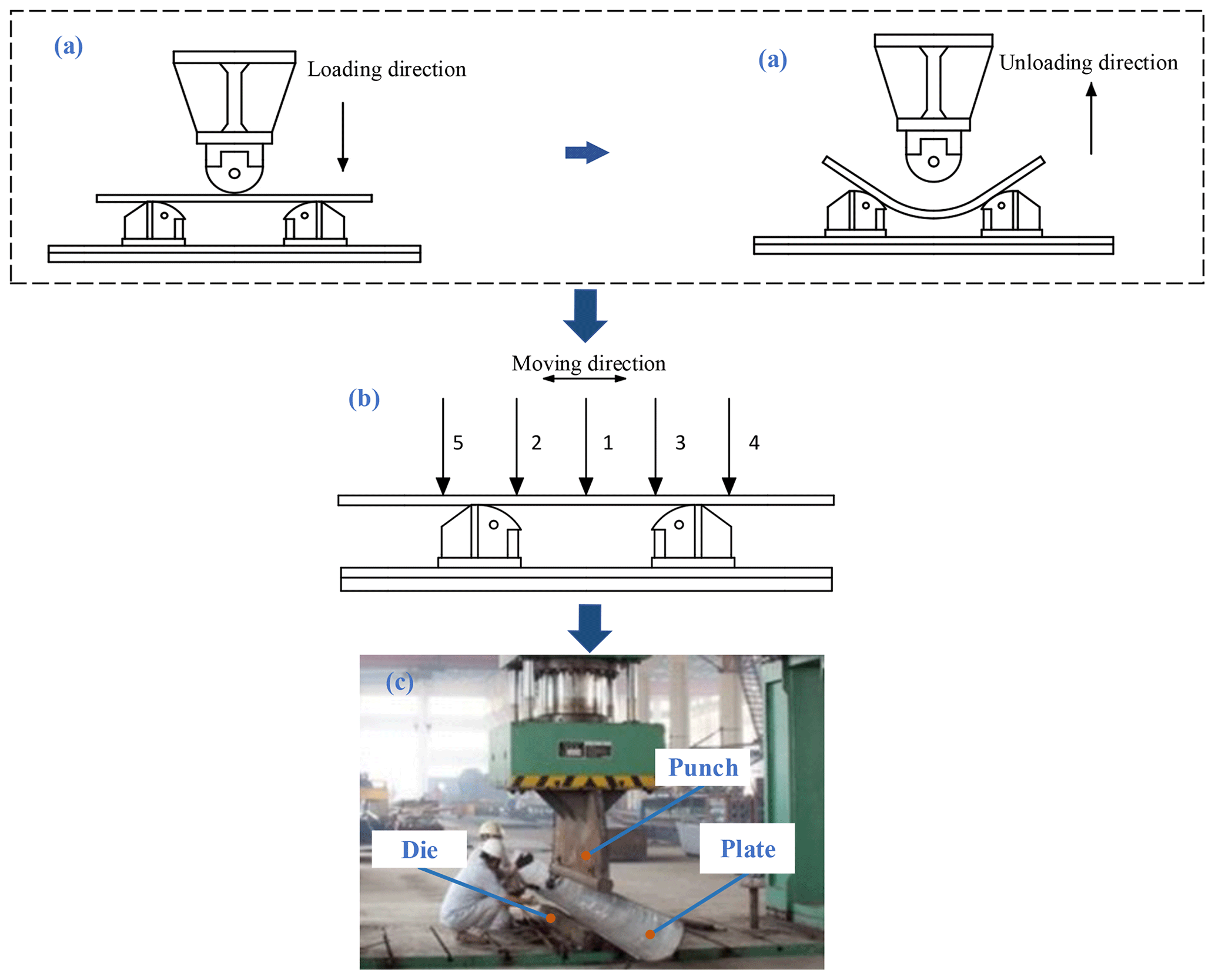
Figure 1 Plate forming by free bending. (a) Principle of forming; (b) processing sequence; (c) ship building process.

In traditional machining, optimal process parameters are determined through empirical methods, implying extreme reliance on the hands-on experience of the skilled worker. The original analytical methods have the disadvantage of lower accuracy. However, the development of finite element technology has made numerical simulation an important method in the study of the springback problem, after plate cold forming (Qiuchong et al., 2016; Shi et al., 2004; Liu et al., 2019). Prior (1994) concluded that the application of explicit and implicit algorithms is very helpful in solving the springback problem. Taherizadeh et al. (2010) showed that a non-associated mixed-hardening model significantly improves the prediction of earing in the cup-drawing forming process and the prediction of springback in the sidewall part of drawn channel sections. Thipprakmas and Rojananan (2008) examined the springback and spring-go phenomena in the V-bending process, using the finite element method (FEM). Trzepiecinski and Lemu (2017) carried out numerical simulation, where they studied the influence of calculation parameters on the springback prediction.

Figure 2 Simplified drawing of local bending.

Figure 3 The shape of 2D plate forming.

The numerical simulation method imposes high requirements on the boundary conditions and requires iterative calculations for complex machining, which takes a long time and requires high performance of the computational equipment. Therefore, it is proposed to use machine learning algorithms to construct a mathematical model, which can accurately describe the real system, providing calculation results similar to the real ones, for analysis purposes, while the prediction or optimization problem is realized on the approximation model (Salais-Fierro et al., 2020; Mucha, 2019). Liu et al. (2007) used the genetic algorithm to optimize a backpropagation neural network (BPNN) and built the springback prediction model of the U-bend of the plate. Froitzheim et al. (2019) established a new artificial neural network model to predict the geometric parameters related to metal sheet forming. Serban et al. (2020) developed an artificial neural network (ANN) model for springback prediction in the case of free cylindrical bending of metal sheets. Yang and Kim (2020) used the optimized BPNN method, based on the genetic algorithm, to predict and optimize the wall angle of the Al3004 sheet with a thickness of 1 mm. Trzepiecinski and Lemu (2020) proposed a cold-rolled anisotropic steel plate springback prediction method, based on the combination of multi-layer perceptron artificial neural network (ANN) and genetic algorithm (GA). Dib et al. (2020) proposed single and ensemble classifiers to predict the springback and maximum thinning of the U channel and the maximum equivalent plastic strain and maximum thinning of the square cup. Guo and Tang (2017) presented a springback bending angle prediction model, based on the combination of error backpropagation neural network and spline function (BPNN-Spline) to rapidly and accurately predict the springback bending angle in the V-die air bending process. It is evident that the machine learning approach is widely used in plate cold forming of different plate types and different machining parameters, providing good prediction results.

In this article, a geometric model, describing the deformation behavior in the local bending process, is established. In addition, global optimization algorithms are used to improve global search ability of BPNN, which is prone to falling into a local optimum. In total, four springback prediction models, based on the GA-BPNN algorithm and the improved particle swarm optimization (PSO)-BPNN algorithms, are established. The comparison of the prediction results of the models to the experimental results verifies the high prediction accuracy of all optimized BPNN models. Especially in the case of local bending, the prediction model, based on the GA-BPNN algorithm, provides a faster solution at less than 10 s. The results show that the prediction model, based on the GA-BPNN algorithm, has higher applicability on the specific research object and selected process parameters of this article.

The rest of this paper is arranged as follows. In Sect. 2, local bending independent and dependent variables are defined, and data are obtained by experiments. In Sect. 3, the related algorithm theory is introduced, and prediction models of optimized BPNN are established. In Sect. 4, five prediction models are evaluated, by comparing coefficient of determination, mean square error, prediction results, errors, and relative errors so as to derive the superiority of GA-BPNN. Finally, the future research direction is pointed out.

2 Experimental procedure

2.1 Material

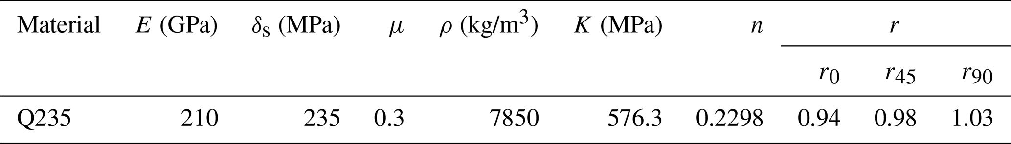
Q235 (structural steel) is widely used in ships, vehicles and containers, due to the moderate carbon content, the superior comprehensive performance, and its well matched properties such as strength, plasticity, and welding. In this paper, Q235 is selected for mechanical performance research, as shown in Table 1, where E is Young's modulus; δ_s is yield strength; μ is Poisson's ratio; ρ is density; K is strengthening factor; n is strain hardening exponent; r is thickness anisotropy coefficient; and r₀, r₄₅, and r₉₀ are the Lankford coefficients obtained at 0, 45, and 90^∘, respectively, according to the rolling direction of the sheet.

Table 1 Mechanical properties of the Q235 plate.

2.2 Method

The experimental principle of plate local bending is shown in Fig. 1a, where a test plate size of 400 mm × 200 mm is illustrated. During the experiment, the stamping head is fed vertically downwards, under the pressure provided by the oil pump, while the plate is displaced along the thickness direction. When unloading, the plate shape changes due to the induced elastic strain recovery. In cases of single curvature surfaces and complex surfaces with small curvature, it is necessary to continuously move the position of the plate and apply multiple local bending deformations, in order to plastically deform it to reach the final target shape, as shown in Fig. 1b and c. In this experiment, only one local bending, in a series of multi-pass local bending deformations, is studied.

2.3 The definition of experimental parameters

The greatest problem of plate local bending is springback, which occurs after unloading and involves many parameters of the actual bending process. The parameters can be distinguished as material parameters, geometric parameters, and process parameters. According to the variable type, there are plate variables, punch variables, die variables, contact surface variable, bending setting variable, and blank holder variables (Table 2). It is very important to study the influence of different factors on the springback of the plate.

Table 2 Influencing factors of springback in local bending.

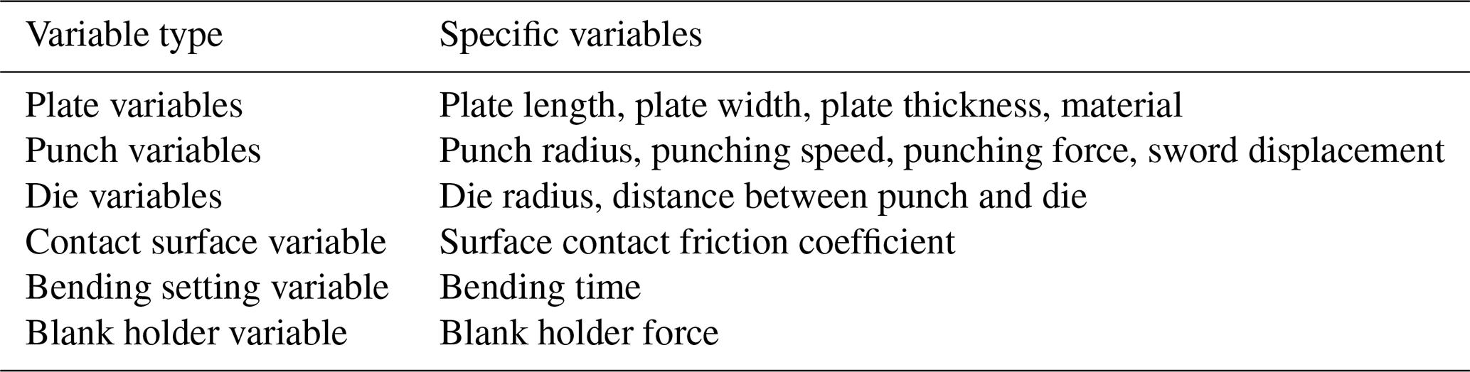
The independent variables are determined based on actual production experience.

1. In local bending, the forming effect is only related to the size of punch and die, so the length and width of the plate are not considered influencing factors.

2. Lindgren (2007) proved that material parameters have an impact on the quality of plate forming, based on finite element analysis, but the plate material in this paper is determined, so it is not considered an influencing factor.

3. The final result of punching speed and force is the sword displacement, which is directly studied in this article.

4. During the cold forming process, the plate and the die are in line, so the die radius is not studied.

5. Since, in the actual local bending process of the plate, the contact surface material and lubrication information is provided, the contact friction coefficient between each component and the plate is determined according to the actual situation, and it is a fixed value in this analysis.

6. The bending time is a fixed value in the analysis in this article.

7. The presence of the blank holder force will cause the plate to become thinner, during the cold bending process, while it may even break if this force is too large. Therefore, this study does not use the blank holder force to ensure the free bending of the plate.

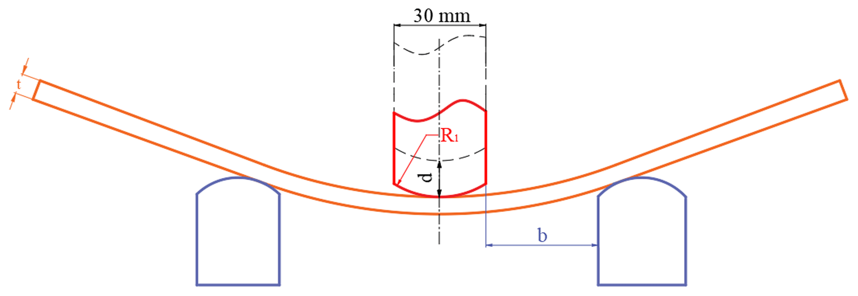
Based on the above analysis, the plate thickness t, the sword displacement d, the distance between the punch and the die b, and the punch radius R₁ are the independent variables as shown in Fig. 2.

Figure 4 System process steps of plate cold forming.

Table 3 Experimental results.

2.4 The definition of springback

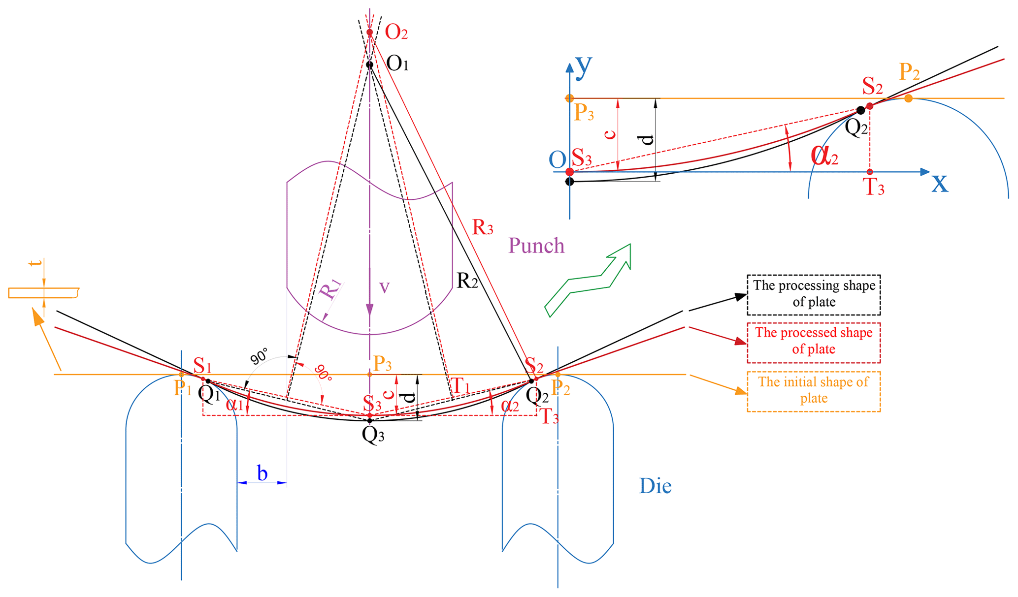
Springback occurs after loading and manifests in three forms: the springback radius increases, the bending angle decreases, and the displacement along the thickness direction becomes smaller, as shown in Fig. 3.

2.4.1 The bending angles α₁ and α₂

Using the lowest point of the processed plate as the origin, the coordinates of points S₂, S₃, andT₃ are (x₁,y₁), (0,0), and (x₁,0), respectively.

$$\begin{array}{}\text{(1)}& {\displaystyle }\tan {\mathit{\alpha }}_{\mathrm{2}}={\displaystyle \frac{{\int }_{\mathrm{0}}^{y_{\mathrm{1}}}\mathrm{d}y}{{\int }_{\mathrm{0}}{}^{x_{\mathrm{1}}}\mathrm{d}x}}={\displaystyle \frac{y_{\mathrm{1}}}{x_{\mathrm{1}}}},\text{(2)}& {\displaystyle }{\mathit{\alpha }}_{\mathrm{2}}=\arctan {\displaystyle \frac{y_{\mathrm{1}}}{x_{\mathrm{1}}}}.\end{array}$$

The bending angle of the right-hand side of the plate α₂ is obtained by Eq. (2), while the bending angle of the left-hand side of the plate α₁ can be obtained in the same way.

Where S₂ is the contact point of the plate and die, S₃ is the midpoint of the plate, T₃ is the pedal, x₁ is the amount of lateral bending deformation, and y₁ is the maximum height difference.

2.4.2 The springback radius R₃

• Step 1: Find the center of circle O₂.

  Consider a straight line, perpendicular to line segment S₂S₃, passing through the midpoint T₁ of this line segment. In the same way, a straight line, passing through the midpoint of S₁S₃ and perpendicular to this line segment, is drawn on the left half. The intersection O₂ of the two straight lines is the center of the circle.

  Where, S₁ is the contact point of the plate and die, O₂ is the center of a circle of curvature radius.

• Step 2: Calculate the springback radius R₃.

  $$\begin{array}{c}{\displaystyle }\text{because}\mathrm{\angle }{S}_{\mathrm{2}}{S}_{\mathrm{3}}{T}_{\mathrm{3}}+\mathrm{\angle }{S}_{\mathrm{3}}{S}_{\mathrm{2}}{T}_{\mathrm{3}}=\mathrm{90}{}^{\circ }\\ {\displaystyle }\mathrm{\angle }{O}_{\mathrm{2}}{S}_{\mathrm{3}}{T}_{\mathrm{1}}+\mathrm{\angle }{S}_{\mathrm{2}}{S}_{\mathrm{3}}{T}_{\mathrm{3}}=\mathrm{90}{}^{\circ }\\ {\displaystyle }\text{therefore}\mathrm{\angle }{O}_{\mathrm{2}}{S}_{\mathrm{3}}{T}_{\mathrm{1}}=\mathrm{\angle }{S}_{\mathrm{3}}{S}_{\mathrm{2}}{T}_{\mathrm{3}}\\ {\displaystyle }\text{because}\mathrm{\angle }{O}_{\mathrm{2}}{T}_{\mathrm{1}}{S}_{\mathrm{3}}=\mathrm{\angle }{S}_{\mathrm{3}}{T}_{\mathrm{3}}{S}_{\mathrm{2}}=\mathrm{90}{}^{\circ }\end{array}$$

According to whether the two angles of one triangle correspond to the two angles of another triangle, the two triangles are similar.

$$\begin{array}{}\text{(3)}& \text{therefore}\mathrm{△}{O}_{\mathrm{2}}{S}_{\mathrm{3}}{T}_{\mathrm{1}}\mathit{\backsim }\mathrm{△}{S}_{\mathrm{3}}{S}_{\mathrm{2}}{T}_{\mathrm{3}}\end{array}$$

Next, the following formulas are derived:

$$\begin{array}{}\text{(4)}& {\displaystyle }{l}_{S_{\mathrm{3}}{T}_{\mathrm{1}}}={\displaystyle \frac{l_{S_{\mathrm{2}}{S}_{\mathrm{3}}}}{\mathrm{2}}}={\displaystyle \frac{\sqrt{{\left(x_{\mathrm{1}}-\mathrm{0}\right)}^{\mathrm{2}}+{\left(y_{\mathrm{1}}-\mathrm{0}\right)}^{\mathrm{2}}}}{\mathrm{2}}},\text{(5)}& {\displaystyle \frac{l_{O_{\mathrm{2}}{S}_{\mathrm{3}}}}{l_{S_{\mathrm{2}}{S}_{\mathrm{3}}}}}={\displaystyle \frac{l_{S_{\mathrm{3}}{T}_{\mathrm{1}}}}{l_{S_{\mathrm{2}}{T}_{\mathrm{3}}}}},\text{(6)}& {\displaystyle }{R}_{\mathrm{3}}=l_{O_{\mathrm{2}}{S}_{\mathrm{3}}}={\displaystyle \frac{l_{S_{\mathrm{3}}{T}_{\mathrm{1}}}}{l_{S_{\mathrm{2}}{T}_{\mathrm{3}}}}}\cdot l_{S_{\mathrm{2}}{S}_{\mathrm{3}}}={\displaystyle \frac{x_{\mathrm{1}}^{\mathrm{2}}+y_{\mathrm{1}}^{\mathrm{2}}}{\mathrm{2}{y}_{\mathrm{1}}}}.\end{array}$$

The specific value of R₃ is calculated, as shown in Eq. (6).

2.4.3 The displacement along the thickness direction c

The displacement in the thickness direction is as follows:

$$\begin{array}{}\text{(7)}& c=l_{P_{\mathrm{3}}{S}_{\mathrm{3}}},\end{array}$$

where P₃ is the midpoint of the initial plate, and S₃ is the midpoint of the plate after springback.

The springback radius R₃ is the most intuitive expression of the physical quantity of springback. In the actual production conditions of a sea vessel, the processing personnel usually uses the sample box or sample plate, to measure the curvature of the hull plate, and the unfitted part is partially processed again, hence the springback radius R₃ is set as a dependent variable.

2.5 Experimental data

There is a group of 28 experiments: the first column indicates the experiment number, the next four columns are features, and the last column is the response. Experimental results rearrange the features according to the order shown in Table 3.

3 Establishment of the machine learning model

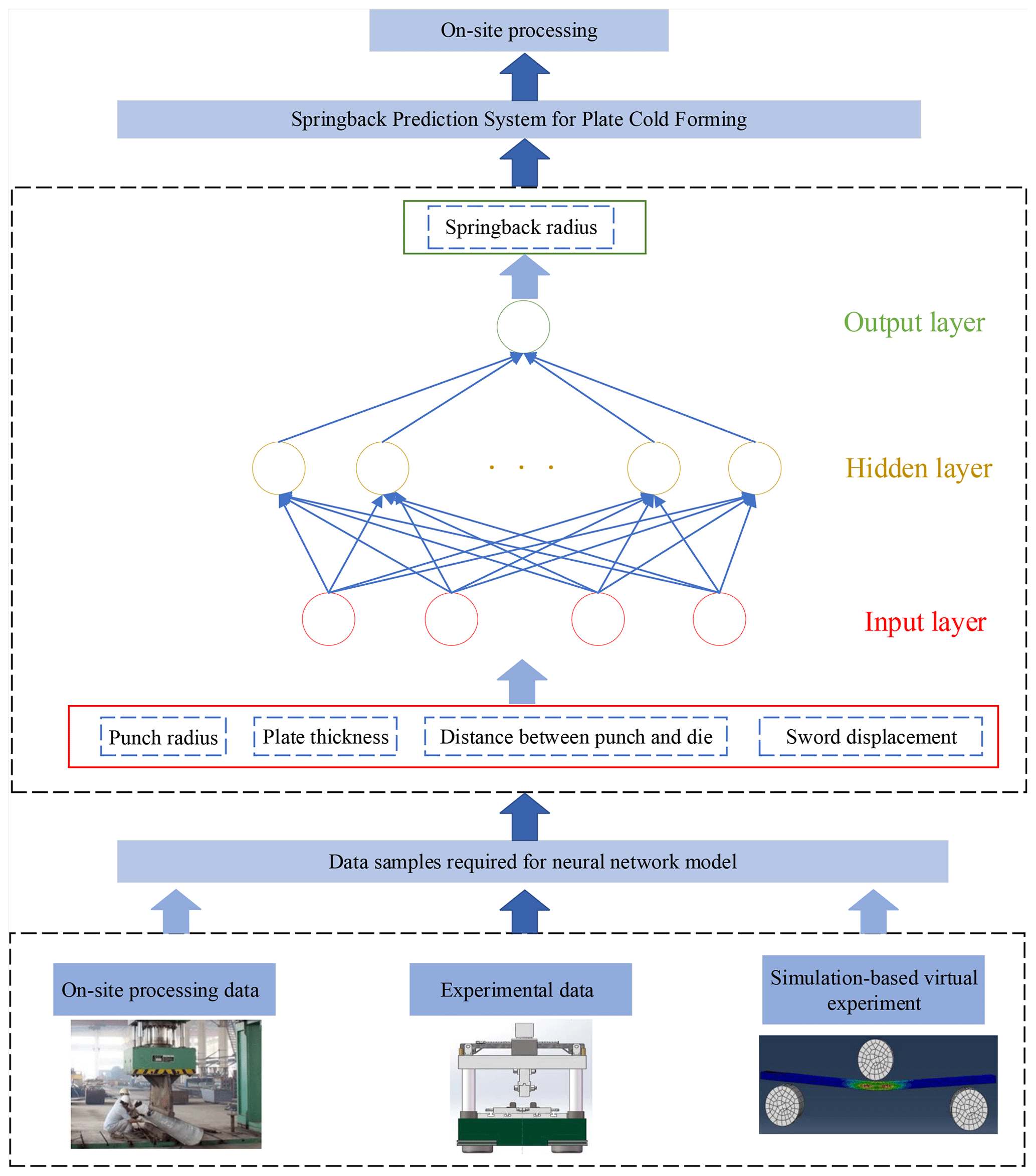
Aiming at the highly nonlinear problem of springback in the case of plate local bending, as affected by many factors, such as material, geometry, and forming process, machine learning algorithms are used to explore the rules between different input variables and output results, in order to calculate a springback prediction and the respective compensation. The BPNN can learn and store a large number of input–output pattern mapping relationships, without the need to reveal the mathematical equation describing this mapping relationship in advance (Miranda et al., 2020). It is suitable for solving multivariable and nonlinear problems, but the BPNN easily falls into a local optimal solution (Inamdar et al., 2000; Kazan et al., 2007; Nasrollahi and Arezoo, 2012; Zhao et al., 2014). This paper proposes an optimized version of BPNN, based on the genetic algorithm and improved particle swarm algorithm, in order to find the global optimal solution. Consequently, by comparing the prediction errors and calculation efficiencies of BPNN based on the genetic algorithm and improved particle swarm algorithm, a better optimization algorithm is selected to make the BPNN reach an accurate prediction by efficient calculation. Furthermore, according to the idea shown in Fig. 4, through on-site processing, experimental processing, and numerical simulation, a large number of sample data are obtained, complementing the construction of the springback prediction system, in order to improve the efficiency of on-site processing.

Figure 5 The flowchart of training BPNN.

3.1 Data preprocessing

• Step 1: Data normalization processing. In order to eliminate the difference between magnitudes, the sample data are normalized and mapped to [0,1], according to the following formula:

  $$\begin{array}{}\text{(8)}& \stackrel{\mathrm{‾}}{x}={\displaystyle \frac{x-x_{min}}{x_{max}-x_{min}}}.\end{array}$$

• Step 2: Train/test split. The last five sets of data in Table 3 are used as testing data, while the remaining data sets are used as training data.

3.2 Backpropagation neural network

The backpropagation neural network (BPNN), proposed by Rumelhart et al. (1986), is a multi-layer feedforward neural network, trained according to the error backpropagation algorithm, which consists of an input layer, a hidden layer, and an output layer.

The ith BP neuron can be expressed as follows:

$$\begin{array}{}\text{(9)}& y_i=f\left(\sum _{j=\mathrm{1}}^n{\mathit{\omega }}_{ij}{x}_j-{\mathit{\theta }}_i\right),\end{array}$$

where x_j is the jth input variable, ω_ij is the neuron weight value, θ_i is the neuron bias value, and y_i is the ith output variable.

The number of hidden layers p is obtained as

$$\begin{array}{}\text{(10)}& p=\sqrt{n+q}+a,\end{array}$$

where n is the number of input layers, q is the number of output layers, and a is an integer and $a\in \left(\mathrm{1},\mathrm{10}\right)$.

The activation function is as follows:

$$\begin{array}{}\text{(11)}& f\left(x\right)={\displaystyle \frac{\mathrm{2}}{\mathrm{1}+e^{-\mathrm{2}x}}}-\mathrm{1}.\end{array}$$

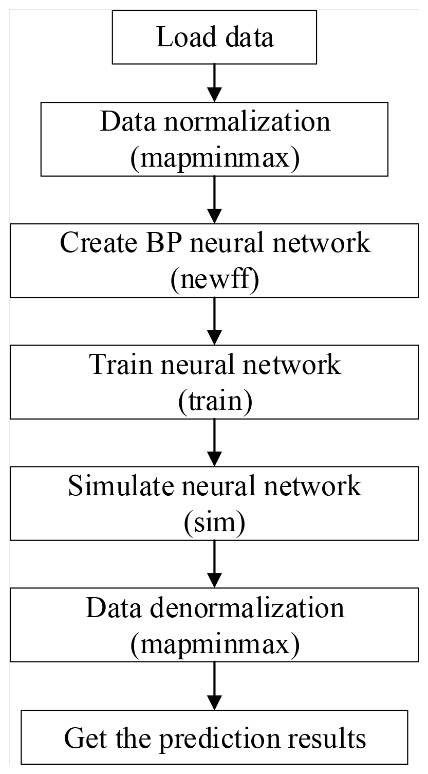
In this paper, the numbers of input layers and output layers are 4 and 1, respectively, while the number of hidden layers is 11. The network training function is Levenberg–Marquardt. The minimum error of the training target is set to 0.001, the number of training sessions is set to 1000, and the learning rate is set to 0.01.

The training process of BPNN is shown in Fig. 5.

Figure 6 The flowchart of optimized BPNN based on the genetic algorithm.

Figure 7 The flowchart of optimized BPNN based on improved particle swarm optimization.

3.3 Genetic algorithm

The genetic algorithm (GA) is an evolutionary algorithm, whose basic principle is to imitate the evolutionary law of natural selection and survival of the fittest in the natural world. It was originally proposed by Holland in 1967 and mainly composed of three basic operations: selection, crossover, and mutation (Liu et al., 2007).

3.4 Particle swarm optimization

Particle swarm optimization (PSO) is a new global optimization algorithm, invented by Eberhart and Kennedy. PSO is an optimization tool, based on iteration, similar to the genetic algorithm. The system is initialized to a set of random solutions, while the optimal value is reached through iteration (Machado et al., 2021). The particle swarm algorithm decides the search path, according to its own speed, whereas it does not have the crossover and mutation operations of the genetic algorithm, as these are added to the particle swarm algorithm at a next step.

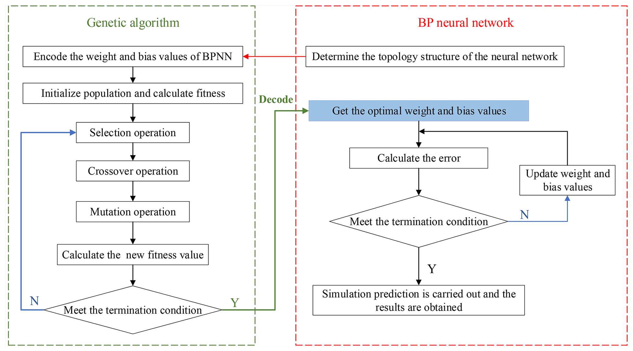
3.5 The BPNN optimized by genetic algorithm

The BPNN optimized by the genetic algorithm (GA-BPNN) mainly uses the genetic algorithm to select a new population generated by replication, crossover, and mutation of individuals with large fitness value, in order to optimize the initial weight and bias values of the BPNN, optimizing the BPNN approach to better predict the output, based on the algorithm flow illustrated in Fig. 6.

The main steps of the genetic algorithm are as follows:

• Step 1: Encode the weight values ω_ij and bias values θ_i of the BPNN to obtain the initial individual, set the population size to 50, and initialize population; the dimension of individual d is as follows:

  $$\begin{array}{}\text{(12)}& d=l\times m+m+m\times n+n,\end{array}$$

  where l is the number of inputs, m is the number of hidden layers, and n is the number of outputs.

• Step 2: Set the maximum number of iterations to 100, and set the reciprocal of the residual sum of squares as the fitness function of the genetic algorithm; the formula is as follows:

  $$\begin{array}{}\text{(13)}& f={\displaystyle \frac{\mathrm{1}}{\sum _{i=\mathrm{1}}^n{\left(y_i-{\widehat{y}}_i\right)}^{\mathrm{2}}}}.\end{array}$$

  (Higher values of f indicate better individual fitness.)

  where f is the fitness function, ${\widehat{y}}_i$ is the predicted value of the ith sample, y_i is the experimental value of the ith sample, and n is the number of samples.

• Step 3: First select the individual with the higher fitness value in the population, as the parent to replicate, and then obtain a new generation of individuals through crossing fragments in individuals; perform mutation operations on the randomly selected individuals to finally obtain a new population.

• Step 4: When the fitness value of the population reaches the maximum fitness value or the maximum number of iterations, the optimization ends; otherwise, return to step 3.

• Step 5: Decode the individual with the maximum fitness value and assign it to the neural network to obtain optimal weight and bias values.

Figure 8 The flowchart of particle swarm optimization based on adaptive mutation.

Figure 9 The flowchart of particle swarm optimization based on natural selection.

3.6 The BPNN optimized by particle swarm algorithm

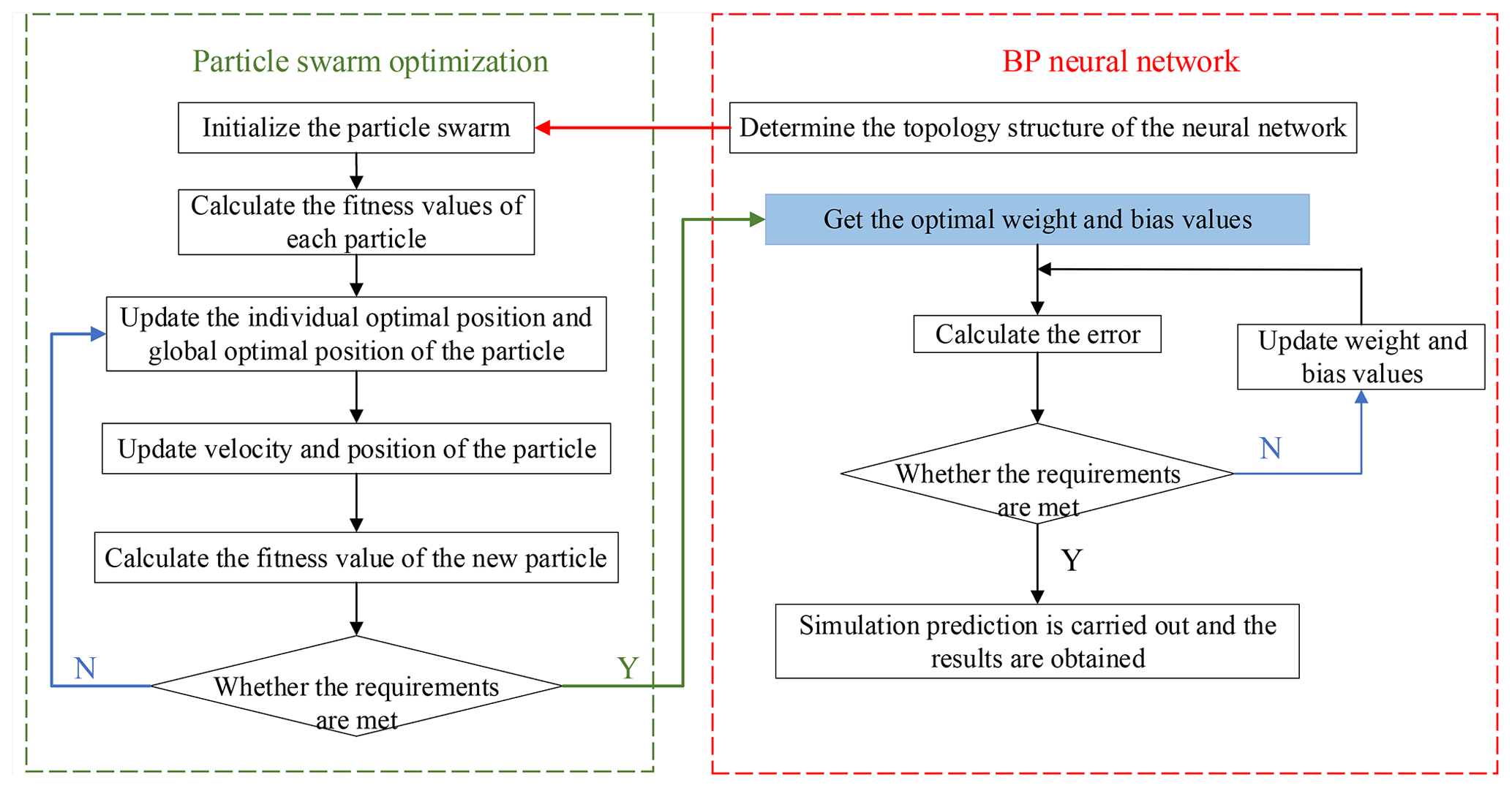
The BPNN, as optimized by the standard particle swarm optimization algorithm (SPSO-BPNN), updates the speed and position of each particle, through the particle swarm algorithm, to obtain the lowest fitness value of the particle, while the position of the particle is assigned to the initial weight and bias values of the BPNN. The algorithm flow is shown in Fig. 7.

The main steps of particle swarm optimization are as follows:

• Step 1: Set the basic parameters of particle swarm algorithm, such as particle position and velocity range, iteration number, inertia factor, learning factor, population size, etc and initialize the initial position and velocity of each particle in the population. The dimension of the particle d is shown in Eq. (12).

• Step 2: Calculate the fitness value of each particle and store its current position and fitness value in the individual best value; store the position and fitness value of the individual with the best fitness value in the global best value. The fitness function is as follows:

  $$\begin{array}{}\text{(14)}& f=\sum _{i=\mathrm{1}}^n\left|y_i-{\widehat{y}}_i\right|,\end{array}$$

  (Lower values of f indicate better fitness of each particle.)

  where f is the fitness function, ${\widehat{y}}_i$ is the predicted value of the ith sample, y_i is the experimental value of the ith sample, and n is the number of samples.

• Step 3: Update the individual optimal position and global optimal position of the particles.

• Step 4: Update the velocity and position of each particle, according to the following formula:

  $$\begin{array}{}\text{(15)}& {\displaystyle }\begin{array}{rl}{\mathit{\nu }}_{ij}(t+\mathrm{1})& =\mathit{\omega }{\mathit{\nu }}_{ij}\left(t\right)+c_{\mathrm{1}}{r}_{\mathrm{1}}\left(t\right)\left[p_{ij}\left(t\right)-x_{ij}\left(t\right)\right]\\ & +c_{\mathrm{2}}{r}_{\mathrm{2}}\left(t\right)\left[p_{gi}\left(t\right)-x_{ij}\left(t\right)\right],\end{array}\text{(16)}& {\displaystyle }{x}_{ij}(t+\mathrm{1})=x_{ij}\left(t\right)+{\mathit{\nu }}_{ij}(t+\mathrm{1}),\text{(17)}& {\displaystyle }\mathit{\omega }={\mathit{\omega }}_{max}-{\displaystyle \frac{\left({\mathit{\omega }}_{max}-{\mathit{\omega }}_{min}\right)\times t}{t_{max}}},\end{array}$$

  where c₁ and c₂ are learning factors, ω is the inertia weight, r₁ and $r_{\mathrm{2}}\in \left(\mathrm{0},\mathrm{1}\right)$ are the random values, p_ij is the particle individual optimal position, p_gi is the global optimal position, x_ij is the current particle position, v_ij is the current particle velocity, ω_max is the maximum inertia weight, ω_min is the minimum inertia weight, t is the current iteration number, and t_max is the maximum iteration number.

  In this paper, $c_{\mathrm{1}}=c_{\mathrm{2}}=\mathrm{2}$, ω_max=0.9, ω_min=0.4, t_max=20, the population size is 20, the particle velocity ranges from −1 to 1, and the particle position ranges from −5 to 5.

  The inertia weight is an important parameter that affects the performance of PSO; the larger it is, the larger the particle velocity changes and the larger the search range of the solution is. Conversely, the smaller the inertia weight is, the smaller the search range of the solution is. Therefore, this paper uses nonlinear inertia weights to improve the convergence speed of the standard particle swarm optimization (SPSO), as follows:

  $$\begin{array}{}\text{(18)}& \mathit{\omega }={\mathit{\omega }}_{max}-\left({\mathit{\omega }}_{max}-{\mathit{\omega }}_{min}\right)\times \tan \left({\displaystyle \frac{t}{t_{max}}}\times {\displaystyle \frac{\mathit{\pi }}{\mathrm{4}}}\right).\end{array}$$

• Step 5: Calculate the fitness value of the new particle and compare the current individual optimal position, individual best fitness value, global optimal position and global best fitness value to the values stored in step 2 and update.

• Step 6: When the fitness value of the population reaches the minimum fitness value or the maximum number of iterations, the optimization ends; otherwise, it returns to step 3.

• Step 7: Assign the position of the particle with the minimum fitness value to the neural network to obtain optimal weight and bias values.

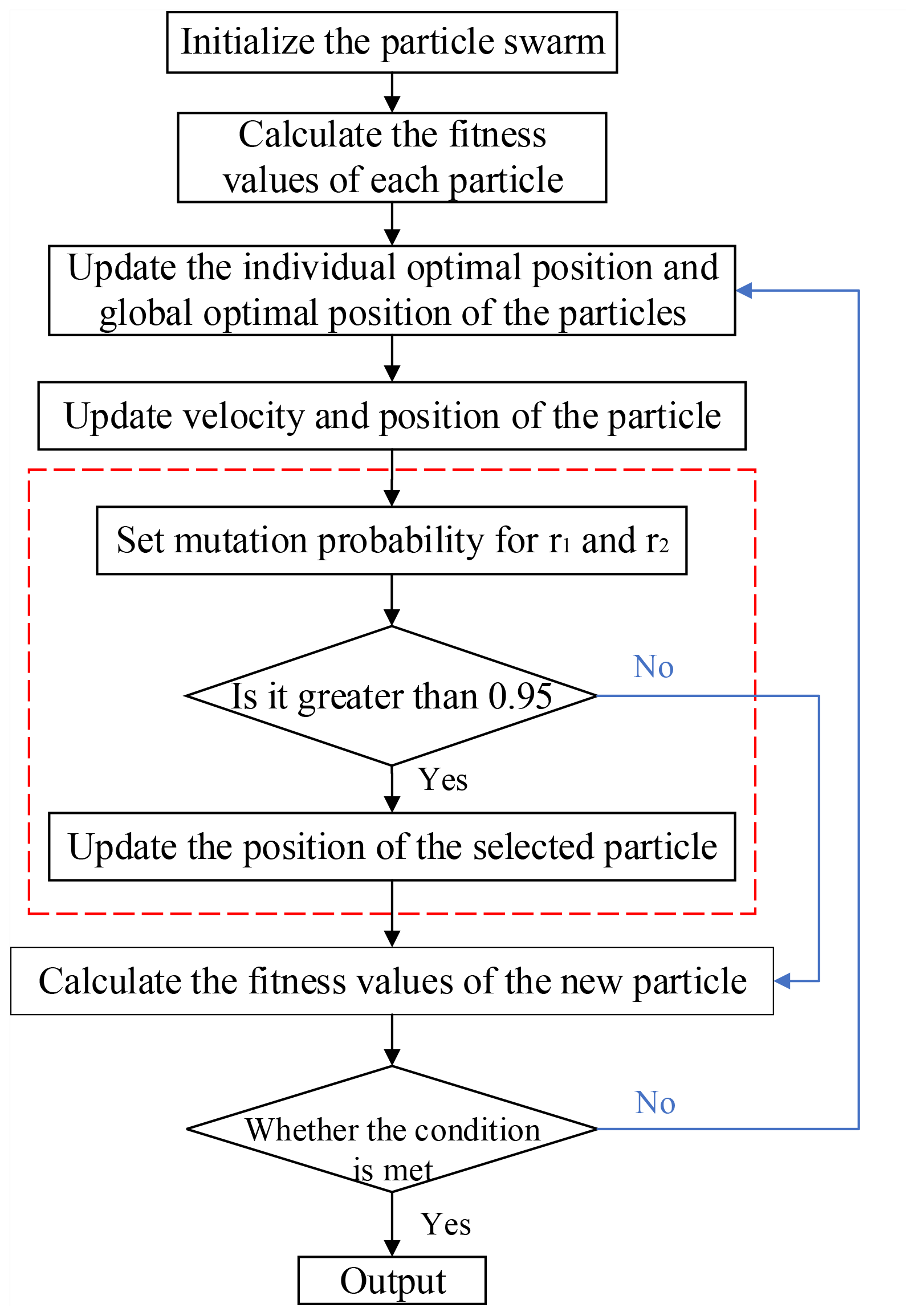
3.6.1 Particle swarm optimization based on adaptive mutation

Particle swarm optimization based on adaptive mutation (APSO) utilizes the mutation principle in genetic algorithm, while the mutation operation is introduced in the particle swarm algorithm in order to reinitialize some particles with a certain probability. Furthermore, the mutation operation can expand the particle search space and maintain particle diversity. If r₁ or r₂ is greater than 0.95, the random particle position will vary. The operation process is as shown in Fig. 8.

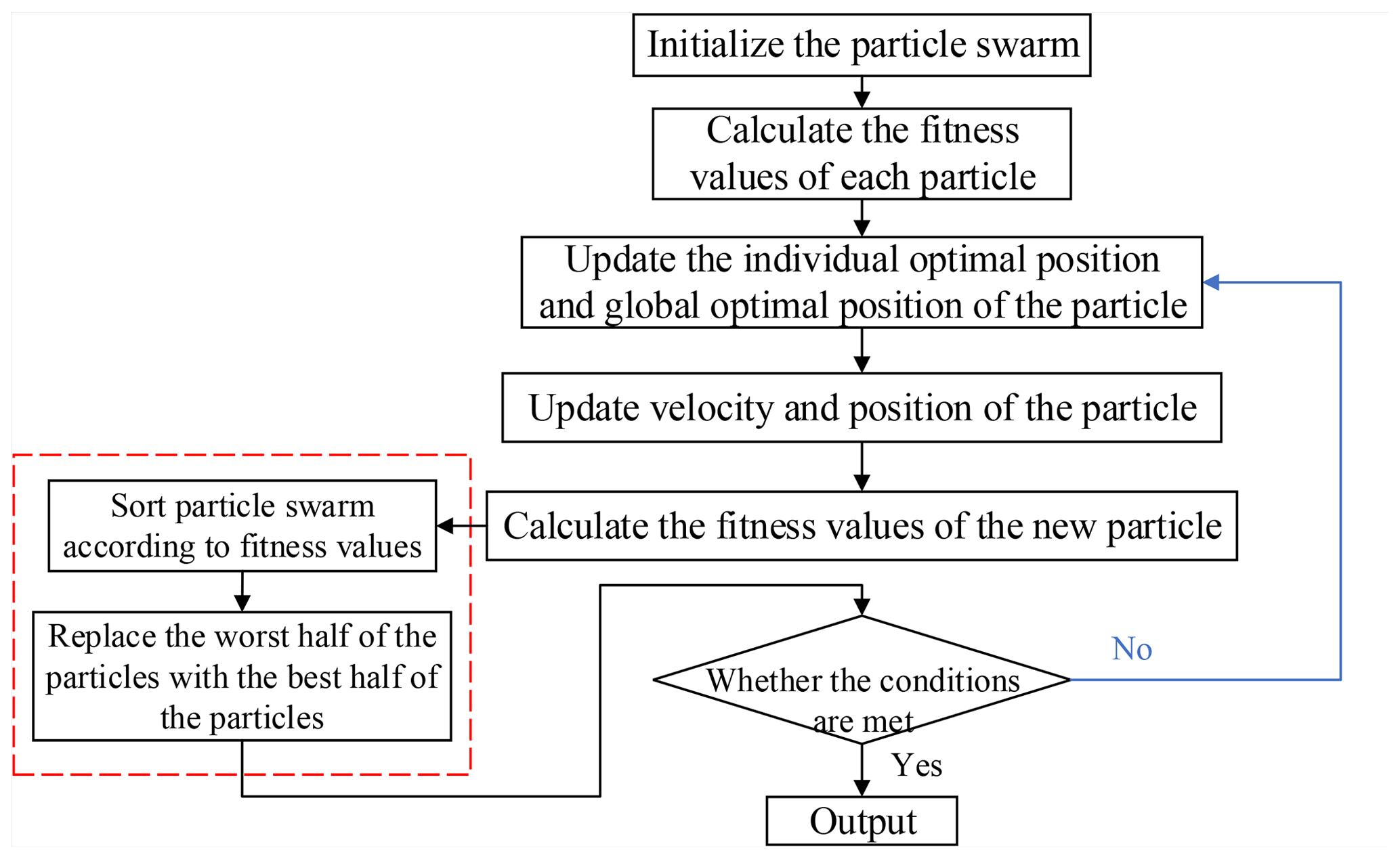
3.6.2 Particle swarm optimization based on natural selection

In this section, the particle swarm optimization, based on the natural selection principle (SelPSO), is described. In each iteration, the particle swarm is sorted according to the fitness value, while the worst half of the particles in the swarm is replaced by the best half, as the original historical optimal value of each individual is retained. The operation process is as shown in Fig. 9.

3.7 Model evaluation index

In order to further evaluate the prediction performance of the model, four indexes are selected: coefficient of determination (R²), mean squared error (MSE), error (Error), and relative error (RE). The respective formulas are as follows:

$$\begin{array}{}\text{(19)}& {\displaystyle }{R}^{\mathrm{2}}={\displaystyle \frac{{\left(n\sum _{i=\mathrm{1}}^n{\widehat{y}}_i\cdot y_i-\sum _{i=\mathrm{1}}^n{\widehat{y}}_i\sum _{i=\mathrm{1}}^n{y}_i\right)}^{\mathrm{2}}}{\left(n\sum _{i=\mathrm{1}}^n{{\widehat{y}}_i}^{\mathrm{2}}-{\left(\sum _{i=\mathrm{1}}^n{\widehat{y}}_i\right)}^{\mathrm{2}}\right)\left(n\sum _{i=\mathrm{1}}^n{y}_i^{\mathrm{2}}-{\left(\sum _{i=\mathrm{1}}^n{y}_i\right)}^{\mathrm{2}}\right)}},\text{(20)}& {\displaystyle }\mathrm{MSE}={\displaystyle \frac{\mathrm{1}}{n}}\sum _{i=\mathrm{1}}^n(y_i-{\widehat{y}}_i{)}^{\mathrm{2}},\text{(21)}& {\displaystyle }\mathrm{Error}=y_i-{\widehat{y}}_i,\text{(22)}& {\displaystyle }\mathrm{RE}={\displaystyle \frac{\left|{\widehat{y}}_i-y_i\right|}{y_i}},\end{array}$$

where ${\widehat{y}}_i$ is the predicted value of the ith sample, y_i is the experimental value of the ith sample, and n is the number of samples.

4 Results and discussion

This paper builds prediction models based on BPNN, GA-BPNN, SPSO-BPNN, APSO-BPNN, and SelPSO-BPNN, each exhibiting prediction performance as shown in Fig. 10.

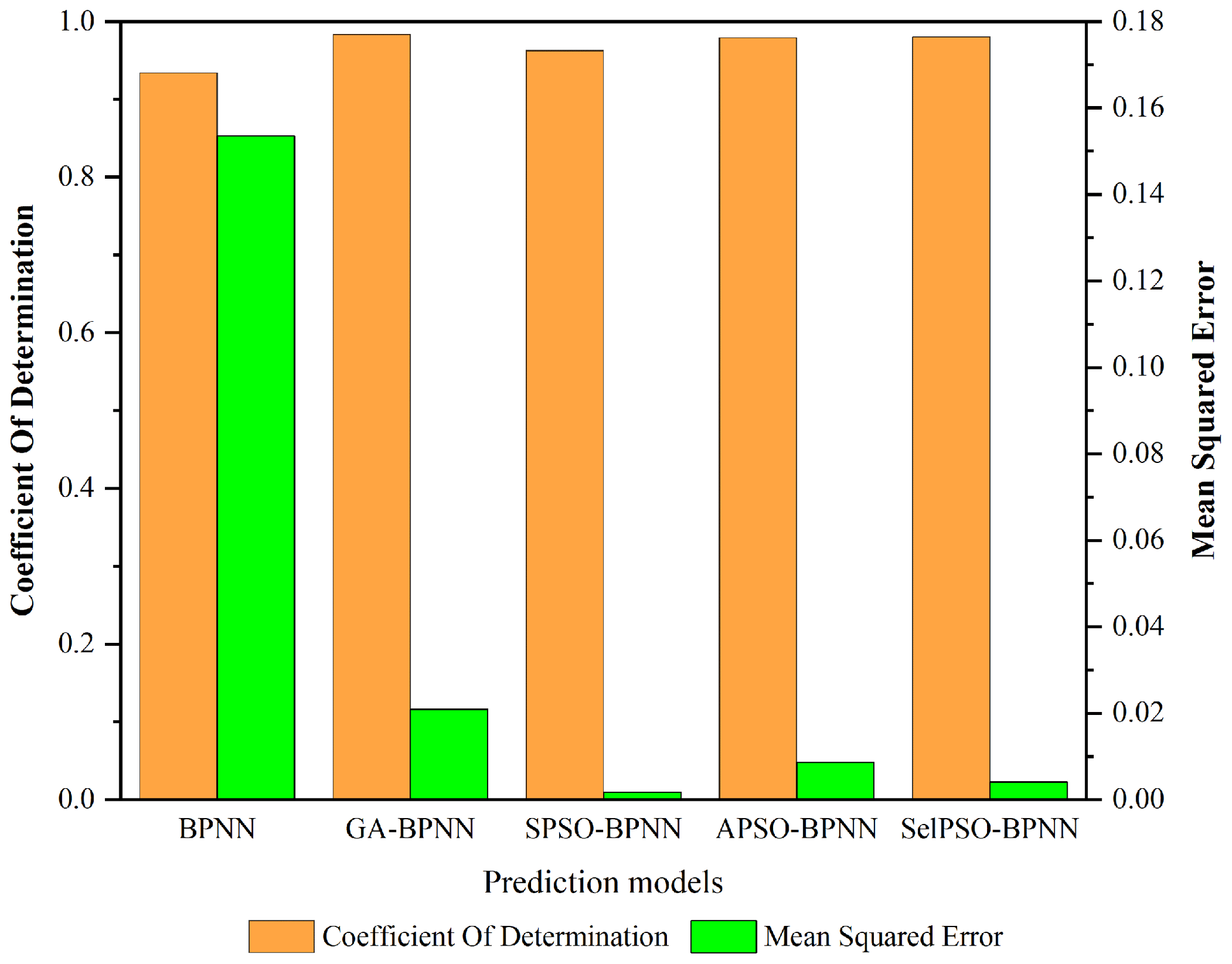
Figure 10 Comparison of coefficient of determination and mean squared error of different models.

Considering that the closer the coefficient of determination is to 1, the better the performance of the model, Fig. 10 shows that all prediction models have a coefficient of determination above 0.9, so all perform well.

The closer the mean square error is to 0, the better the performance of the model. Figure 10 illustrates that excluding the initial BPNN, where the magnitude of mean square error is, the other four magnitudes of mean square error are 10⁻² or 10⁻³. Given that the overall value is below 0.16, the performance of all five prediction models is rated as good.

In summary, the five abovementioned prediction models are trained to achieve the best performance.

The prediction results and the errors between the experimental values and the predicted values of five prediction models are shown in Figs. 11 and 12.

Figure 11 Comparison of the prediction results of different models.

Figure 12 Comparison of errors of different models.

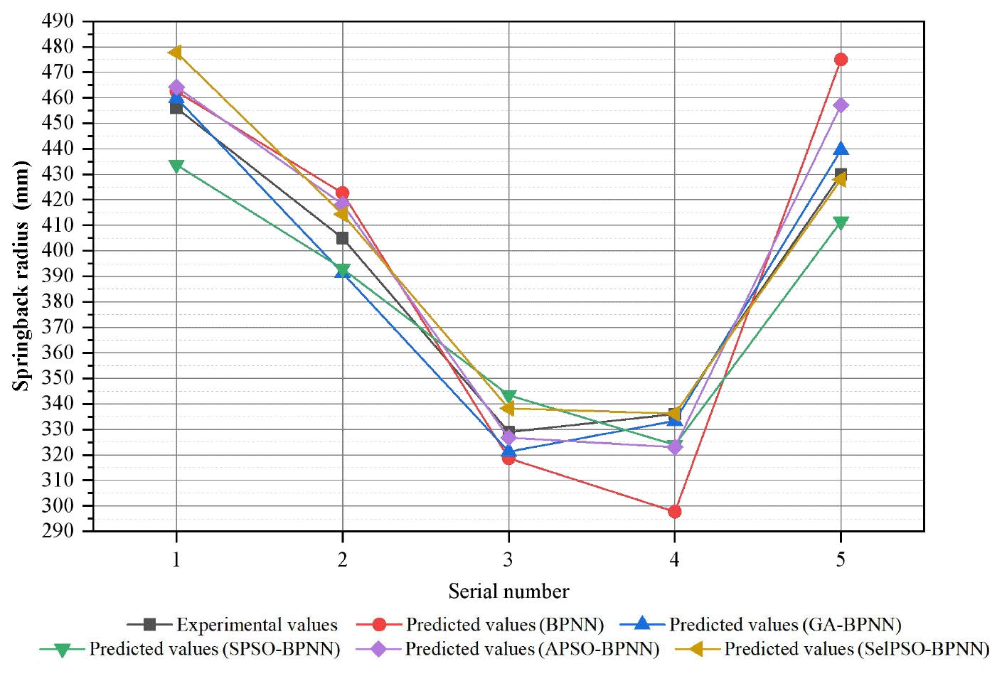
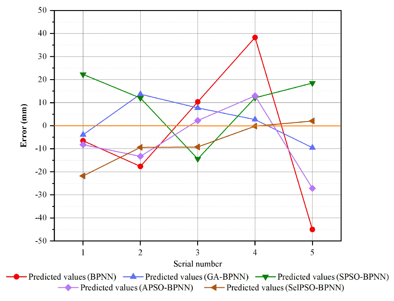
Figure 11 shows that the prediction results of the five prediction models roughly fit the experimental values, without every model's prediction effect meeting the requirements. In Fig. 12, the maximum error of BPNN reaches 45.0094 mm and the minimum error is at 6.5425 mm. The average error is equal to 23.45 mm, which is significantly higher than the average error of the other four models. Obviously it does not find the global optimal solution. The maximum errors of the other four algorithms are all within 30 mm, and their average error is less than 16 mm, so the initial BPNN prediction effect is not better than that of the other models. Moreover, the average error of the prediction model, based on GA-BPNN, is 7.5 mm, which is the lowest among all models.

The difference in order of magnitude of each experimental value is different, so it is not comprehensive to characterize the accuracy of the model by the error alone.

The relative errors of five prediction models are shown in Fig. 13.

Figure 13 Comparison of relative errors of different models.

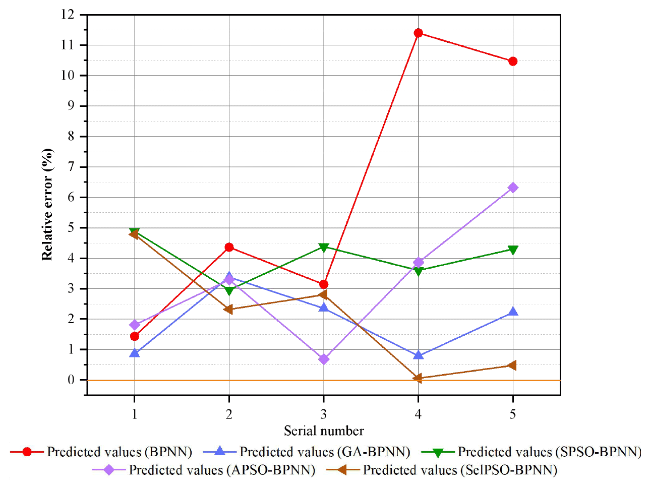
The smaller the relative error, the better the prediction effect. According to Fig. 13, the average relative error of BPNN is 6.16 %, and the maximum relative error is 11.4 %, which is far worse than in other algorithms. The average relative error of SPSO-BPNN is 4.024 %, the average relative error of APSO-BPNN is 3.192 %, and the average relative error of SelPSO-BPNN is 2.087 %; SPSO-BPNN has the worst prediction accuracy, so improving its global search capability by optimizing the SPSO algorithm is of actual essence. The average relative errors of GA-BPNN and SelPSO-BPNN are 1.92 % and 2.087 %, respectively, as they both exhibit good prediction accuracy. Given that efficiency is a very important factor, one should note that the calculation time of GA-BPNN is less than 10 s, while the calculation time of SelPSO-BPNN is less than 52 s. In summary, GA-BPNN is more suitable for solving the specific problems, as raised in this study.

5 Conclusions

Aiming at the key issues of effective prediction and compensation of springback in plate local bending, this paper proposes a springback prediction technology, based on an improved machine learning algorithm model, which provides guidance for accurate prediction and efficient springback calculation. The main conclusions obtained are as follows:

1. Considering the BPNN as the basic framework, optimized prediction models are obtained by adding GA, PSO, and improved PSO. By comparison, it is found that the prediction model, based on the GA-BPNN algorithm, is more suitable for the springback prediction problem of the geometrical and process parameters, as these are selected in this paper.

2. Considering the local bending process of the plate as the object, the application of the machine learning model in springback prediction and compensation is realized. The prediction model, based on GA-BPNN, has a coefficient of determination of 0.98 and a mean square error of 0.020865. The average error is 7.5 mm, the average relative error is 1.92 %, and the calculation time is less than 10 s, indicating high prediction accuracy and high calculation efficiency.

3. The research object of this paper is a single curvature plate, and the results apply only to small samples and a small amount of input. In a follow-up study, more material properties will be added to increase the amount of input, and simulation-based virtual experiments will be introduced to increase the sample size, in order to study the double-curvature plate on the basis of the proposed prediction models.