Design optimization of vehicle asynchronous motors based on fractional harmonic response analysis

To make vehicles more reliable and efficient, many researchers have tried to improve the rotor performance. Although certain achievements have been made, the previous finite element model did not reflect the historical process of the motor rotor well, and the rigidity and mass in rotor optimization are less discussed together. This paper firstly introduces fractional order into a finite element model to conduct the harmonic response analysis. Then, we propose an optimal design framework of a rotor. In the framework, objective functions of rigidity and mass are defined, and the relationship between high rigidity and the first-order frequency is discussed. In order to find the optimal values, an accelerated optimization method based on response surface (ARSO) is proposed to find the suitable design parameters of rigidity and mass. Because the higher rigidity can be transformed into the first-order natural frequency by objective function, this paper analyzes the first-order frequency and mass of a motor rotor in the experiment. The results proved that not only is the fractional model effective, but also the ARSO can optimize the rotor structure. The first-order natural frequency of asynchronous motor rotor is increased by 11.2 %, and the mass is reduced by 13.8 %, which can realize high stiffness and light mass of asynchronous motor rotors.

1 Introduction

Electric vehicles appear to be one of the viable choices in face of the world's increasing attention to environmental protection, energy shortage and other issues (Emadi et al., 2008; Arhun et al., 2018a; Migal et al., 2019). Therefore, it is necessary to design and optimize vehicle monitors. Among the various kinds of electric monitors, induction motors have been widely used because of better performance (Dvadnenko et al., 2018; Francis et al., 2019; Hnatov et al., 2019; Zarma et al., 2019). High reliability and high efficiency are its main characteristics of induction motor (Benbouzid, 1999). For induction motors, it is reported that the failure rate is from stator, bearing, rotor and other aspects (O'Donnell, 2007; Benbouzid and Kliman, 2003; Yildirim et al., 2014; Albrecht et al., 1986).

Reducing the vibration effect of motors can improve the reliability, durability and service life of a motor. In order to achieve this, it is usual to analyze the natural frequency of the motor. The natural frequency can be obtained by numerical methods or modal test experiments (Ewins, 1985; Arhun et al., 2018b). Much research has been proposed in recent years. Ma et al. (2015) proposed an analysis method to study the vibration characteristics of an asymmetric and anisotropic rotor-bearing system. By establishing a linear differential equation with periodic coefficients, the calculation efficiency was improved, and the results were also verified by experimental studies. They suggested to investigate the frequency characteristics and stability of asymmetric anisotropic rotor-bearing systems. Modifications are made to incorporate the effect of stator asymmetry into an existing three-dimensional (3D) solid finite element procedure. In the research of Yin et al. (2020), a specially designed modal conversion horn with an oblique beam was applied. They transferred the longitudinal vibration to an additional bending vibration. Modal analysis was conducted to illustrate the elliptical vibration process by the finite element method. Then the output performance of the motor was evaluated via a series of experiments. Widdle et al. (2006) proposed a model for high-frequency torsional vibration analysis. The research of Li et al. (2008) studied the nonlinear vibration of a three-phase AC motor-linkage mechanism system with links fabricated from three-dimensional braided composite materials. Migal et al. (2021) described a method to select an asynchronous traction electric drive for an electric vehicle that enables the assessment of necessary technical, environmental and operational qualities.

In general, the prior studies have made progress on vibration modal analysis and design optimization of motor, but there is still room for improvement. Firstly, the built finite element model does not consider the historical process of the motor rotor well. Therefore, it cannot accurately reflect the actual dynamic characteristics of the motor. Moreover, most of the existing methods discussed the motor performance by considering frequency, but fewer involved the research of considering the mass and rigidity together. To improve the above situations, this paper combines the fractional harmonic response (Wang and Jiang, 2018; Yan et al., 2020) to the finite element model that can have the dynamic characteristic. Then, we set the high rigidity and the light mass as the optimization objectives. By analyzing the relationship between rigidity and first-order frequency, we transform the optimization into the first-order frequency and the mass. In order to find optimal values, an accelerated optimization method based on response surface (ARSO) is proposed in this paper, and three intelligent optimization algorithms – including traversal search algorithm (TS) (Fang and Xu, 2017), multi-objective genetic algorithm (MOGA) (Ponnambalam et al., 2000) and optimization algorithm based on response surface (RSO) (Munck et al., 2008) – are selected for comparison. Finally, experimental results are given to prove the effectiveness of our proposed approach.

The paper is organized as follows: Sect. 2 presents the fractional finite element model of rotor support casing. In Sect. 3, the design optimization of asynchronous motor rotor is described. Section 4 shows the experimental results. Section 5 is optimization analysis, and discussion is given in Sect. 6. Section 7 concludes this paper.

2 Fractional rotor response system

2.1  Definition of fractional derivative

As defined in the work by Scherer et al. (2011), the Grünwald–Letnikov definition shows an expression for qth derivative, where $q\in R^{+}$. In addition, it allows one to consider the so-called short-memory principle as follows.

$$\begin{array}{}\text{(1)}& {}_a{D}_t^{q}f\left(t\right)={\lim }_{h\to \mathrm{0}}{\displaystyle \frac{\mathrm{1}}{h^q}}\sum _{j=\mathrm{0}}^{\left[\frac{t-a}{h}\right]}(-\mathrm{1}{)}^j\left({}_j^q\right)f(t-jh),\end{array}$$

where $(-\mathrm{1}{)}^j{(}_j^q)$ represents binomial coefficients, $c_j^q$ for $j=\mathrm{0},\mathrm{1},\mathrm{2},\mathrm{\dots }$, which are given by

$$\begin{array}{}\text{(2)}& c_{\mathrm{0}}^q=\mathrm{1},c_j^q=\left(\mathrm{1}-{\displaystyle \frac{\mathrm{1}+q}{j}}\right)c_{j-\mathrm{1}}^q.\end{array}$$

Based on Eq. (1), the solution of a fractional differential equation given by ${}_a{D}_t^{q}y\left(t\right)=f\left(y\right(t),t)$ is defined as $y\left(t_k\right)=f\left(y\right(t_k),t_k)h^q-{\sum }_{j=v}^k{c}_j^{q}y\left(t_{k-j}\right)$, where t_k=kh, h is the time step, and v follows the rule

$$\begin{array}{}\text{(3)}& v=\left\{\begin{array}{cc}\mathrm{1}& \text{for}k\le \frac{L_{\mathrm{m}}}{h}\\ \lfloor k-\frac{L_{\mathrm{m}}}{h}\rfloor & \text{for}k>\frac{L_{\mathrm{m}}}{h}\end{array}\right.,\end{array}$$

with L_m being the memory length, which can be set according to the required accuracy.

2.2 Model description

Figure 1 describes the finite element rotor model. The rotor can be divided into common beam elements, including elastic shaft, distributed mass and stiff plate. N nodes and M plates are contained in the rotor. As seen in Fig. 1, the elastic modulus, area moment of inertia, shear modulus, Poisson ratio, shaft length, shaft density and shaft cross-sectional area are represented by E, I, G, μ, L, ρ and A, respectively. For disc P_i, J_ddi, m_rpi and J_pdi are equatorial moment of inertia, disc mass and pole moment of inertia, respectively. F_xi and F_yi represent the force of the i node, and the moments of the i node are described by M_xi and M_yi. In the coordinate system, the position of the elastic center line is decided by the displacements of x(s,t) and y(s,t); (s,t) angles of x and y can be used to obtain the orientation of the cross-section.

Figure 1 Finite element rotor model.

Now the equation of rigid motion is introduced. m_p, J_dd, J_pd and ω are set to represent the plate mass, moment of inertia of the Equator, the moment of inertia of the pole and rotational angular velocity of plate, respectively. By Lagrangian theorem, the equation of rigid motion is given as follows.

$$\begin{array}{}\text{(4)}& \left(M_{\mathrm{td}}+M_{\mathrm{rd}}\right){\ddot{q}}_{\mathrm{d}}-\mathit{\omega }{G}_{\mathrm{d}}{\dot{q}}_{\mathrm{d}}=Q_{\mathrm{d}},\end{array}$$

where M_td and M_rd are mass matrix and mass inertia matrix. G_d is the gyro matrix, and $q_{\mathrm{d}}=[x,y,\mathit{\varphi },\mathit{\psi }]$ is the generalized displacement vector. Q_d is generalized external force vector. Then, M_td, M_rd and G_d are given:

$$\begin{array}{}\text{(5)}& {\displaystyle }{M}_{\mathrm{td}}=\left[\begin{array}{cccc}{m}_{\mathrm{p}}& \mathrm{0}& \mathrm{0}& \mathrm{0}\\ \mathrm{0}& m_{\mathrm{p}}& \mathrm{0}& \mathrm{0}\\ \mathrm{0}& \mathrm{0}& \mathrm{0}& \mathrm{0}\\ \mathrm{0}& \mathrm{0}& \mathrm{0}& \mathrm{0}\end{array}\right],\text{(6)}& {\displaystyle }{M}_{\mathrm{rd}}=\left[\begin{array}{cccc}\mathrm{0}& \mathrm{0}& \mathrm{0}& \mathrm{0}\\ \mathrm{0}& \mathrm{0}& \mathrm{0}& \mathrm{0}\\ \mathrm{0}& \mathrm{0}& J_{\mathrm{dd}}& \mathrm{0}\\ \mathrm{0}& \mathrm{0}& \mathrm{0}& J_{\mathrm{dd}}\end{array}\right],\text{(7)}& {\displaystyle }{G}_{\mathrm{d}}=\left[\begin{array}{cccc}\mathrm{0}& \mathrm{0}& \mathrm{0}& \mathrm{0}\\ \mathrm{0}& \mathrm{0}& \mathrm{0}& \mathrm{0}\\ \mathrm{0}& \mathrm{0}& \mathrm{0}& -J_{\mathrm{pd}}\\ \mathrm{0}& \mathrm{0}& J_{\mathrm{pd}}& \mathrm{0}\end{array}\right].\end{array}$$

Next, the equation of beam motion is described secondly. E, G, μ, d, D and L are set as the element modulus of elasticity, the shear modulus, the Poisson ratio, the inner diameter, the outer diameter and the length, and then I is calculated:

$$\begin{array}{}\text{(8)}& I={\displaystyle \frac{\mathit{\pi }}{\mathrm{64}}}\left(D^{\mathrm{4}}-d^{\mathrm{4}}\right).\end{array}$$

The cross-sectional area A

$$\begin{array}{}\text{(9)}& A={\displaystyle \frac{\mathit{\pi }}{\mathrm{4}}}\left(D^{\mathrm{2}}-d^{\mathrm{2}}\right).\end{array}$$

The effective shear area A_s

$$\begin{array}{}\text{(10)}& A_{\mathrm{s}}={\displaystyle \frac{A}{\frac{\mathrm{10}}{\mathrm{9}}\left(\mathrm{1}+\frac{\mathrm{1.6}D\times d}{D^{\mathrm{2}}+d^{\mathrm{2}}}\right)}}.\end{array}$$

or

$$\begin{array}{}\text{(11)}& A_{\mathrm{s}}={\displaystyle \frac{A}{\frac{\mathrm{7}+\mathrm{6}\mathit{\mu }}{\mathrm{6}(\mathrm{1}+\mathit{\mu })}\left[\mathrm{1}+\frac{\mathrm{20}+\mathrm{12}\mathit{\mu }}{\mathrm{7}+\mathrm{6}\mathit{\mu }}{\left(\frac{D\times d}{D^{\mathrm{2}}+d^{\mathrm{2}}}\right)}^{\mathrm{2}}\right]}}.\end{array}$$

Shear deformation coefficient ϕ_s

$$\begin{array}{}\text{(12)}& {\mathit{\varphi }}_{\mathrm{s}}={\displaystyle \frac{\mathrm{12}EI}{G{A}_{\mathrm{s}}{L}^{\mathrm{2}}}}.\end{array}$$

For a beam element, two nodes, 8 degrees of freedom, and 8 degrees of freedom are contained. Then the cross-sectional displacement of the unit as a function of time can be seen as a function of the position along the axis of the unit. Therefore, the generalized displacement of the unit endpoint with time change can be described by

$$\begin{array}{}\text{(13)}& q_{\mathrm{e}}\left(t\right)={\left[\begin{array}{llllllll}{q}_{\mathrm{1}\mathrm{e}}& q_{\mathrm{2}\mathrm{e}}& q_{\mathrm{3}\mathrm{e}}& q_{\mathrm{4}\mathrm{e}}& q_{\mathrm{5}\mathrm{e}}& q_{\mathrm{6}\mathrm{e}}& q_{\mathrm{7}\mathrm{e}}& q_{\mathrm{8}\mathrm{e}}\end{array}\right]}^{\mathrm{T}}.\end{array}$$

According to Lagrange theorem, the equation of motion of the beam is as follows:

$$\begin{array}{}\text{(14)}& \left(M_{\mathrm{te}}+M_{\mathrm{re}}\right){\ddot{q}}_{\mathrm{e}}+\left(-\mathit{\omega }{G}_{\mathrm{e}}\right){\dot{q}}_{\mathrm{e}}+\left(K_{\mathrm{be}}-K_{\mathrm{ce}}\right)q_{\mathrm{e}}=Q_{\mathrm{e}},\end{array}$$

where Q_e is the generalized external force vector, M_te and M_re are mass matrix and mass inertia matrix, G_e is gyro matrix, K_be is shearing stiffness matrix, and K_ae is the unit tensile stiffness matrix. The corresponding calculation process is given in Eqs. (19)–(24).

$$\begin{array}{}\text{(15)}& {\displaystyle }\begin{array}{rl}{M}_{\mathrm{te}}& ={\displaystyle \frac{\mathit{\rho }L}{{\left(\mathrm{1}+{\mathit{\varphi }}_{\mathrm{s}}\right)}^{\mathrm{2}}}}\\ & \cdot \left[\begin{array}{cccccccc}{M}_{\mathrm{t}\mathrm{1}}& \mathrm{0}& \mathrm{0}& M_{\mathrm{t}\mathrm{4}}& M_{\mathrm{t}\mathrm{3}}& \mathrm{0}& \mathrm{0}& -M_{\mathrm{t}\mathrm{5}}\\ \mathrm{0}& M_{\mathrm{t}\mathrm{1}}& -M_{\mathrm{t}\mathrm{4}}& \mathrm{0}& \mathrm{0}& M_{\mathrm{t}\mathrm{3}}& M_{\mathrm{t}\mathrm{5}}& \mathrm{0}\\ \mathrm{0}& -M_{\mathrm{t}\mathrm{4}}& M_{\mathrm{t}\mathrm{2}}& \mathrm{0}& \mathrm{0}& -M_{\mathrm{t}\mathrm{5}}& M_{\mathrm{t}\mathrm{6}}& \mathrm{0}\\ M_{\mathrm{t}\mathrm{4}}& \mathrm{0}& \mathrm{0}& M_{\mathrm{t}\mathrm{2}}& M_{\mathrm{t}\mathrm{5}}& \mathrm{0}& \mathrm{0}& M_{\mathrm{t}\mathrm{6}}\\ M_{\mathrm{t}\mathrm{3}}& \mathrm{0}& \mathrm{0}& M_{\mathrm{t}\mathrm{5}}& M_{\mathrm{t}\mathrm{5}}& \mathrm{0}& \mathrm{0}& -M_{\mathrm{t}\mathrm{4}}\\ \mathrm{0}& M_{\mathrm{t}\mathrm{3}}& -M_{\mathrm{t}\mathrm{5}}& \mathrm{0}& \mathrm{0}& M_{\mathrm{t}\mathrm{1}}& M_{\mathrm{t}\mathrm{4}}& \mathrm{0}\\ \mathrm{0}& M_{\mathrm{t}\mathrm{5}}& M_{\mathrm{t}\mathrm{6}}& \mathrm{0}& \mathrm{0}& M_{\mathrm{t}\mathrm{4}}& M_{\mathrm{t}\mathrm{2}}& \mathrm{0}\\ -M_{\mathrm{t}\mathrm{5}}& \mathrm{0}& \mathrm{0}& M_{\mathrm{t}\mathrm{6}}& -M_{\mathrm{t}\mathrm{4}}& \mathrm{0}& \mathrm{0}& M_{\mathrm{t}\mathrm{2}}\end{array}\right],\end{array}\text{(16)}& {\displaystyle }\begin{array}{rl}& M_{\mathrm{t}\mathrm{1}}={\displaystyle \frac{\mathrm{13}}{\mathrm{15}}}+{\displaystyle \frac{\mathrm{7}}{\mathrm{10}}}{\mathit{\varphi }}_{\mathrm{s}}+{\displaystyle \frac{\mathrm{1}}{\mathrm{3}}}{\mathit{\varphi }}_{\mathrm{s}}^{\mathrm{2}},\\ & M_{\mathrm{t}\mathrm{2}}=\left({\displaystyle \frac{\mathrm{1}}{\mathrm{105}}}+{\displaystyle \frac{\mathrm{1}}{\mathrm{60}}}{\mathit{\varphi }}_{\mathrm{s}}+{\displaystyle \frac{\mathrm{1}}{\mathrm{120}}}{\mathit{\varphi }}_{\mathrm{s}}^{\mathrm{2}}\right)L^{\mathrm{2}},\\ & M_{\mathrm{t}\mathrm{3}}={\displaystyle \frac{\mathrm{9}}{\mathrm{70}}}+{\displaystyle \frac{\mathrm{3}}{\mathrm{10}}}{\mathit{\varphi }}_{\mathrm{s}}+{\displaystyle \frac{\mathrm{1}}{\mathrm{6}}}{\mathit{\varphi }}_{\mathrm{s}}^{\mathrm{2}},\\ & M_{\mathrm{t}\mathrm{4}}=\left({\displaystyle \frac{\mathrm{11}}{\mathrm{210}}}+{\displaystyle \frac{\mathrm{11}}{\mathrm{120}}}{\mathit{\varphi }}_{\mathrm{s}}+{\displaystyle \frac{\mathrm{1}}{\mathrm{24}}}{\mathit{\varphi }}_{\mathrm{s}}^{\mathrm{2}}\right)L,\\ & M_{\mathrm{t}\mathrm{5}}=\left({\displaystyle \frac{\mathrm{13}}{\mathrm{420}}}+{\displaystyle \frac{\mathrm{3}}{\mathrm{40}}}{\mathit{\varphi }}_{\mathrm{s}}+{\displaystyle \frac{\mathrm{1}}{\mathrm{24}}}{\mathit{\varphi }}_{\mathrm{s}}^{\mathrm{2}}\right)L,\\ & M_{\mathrm{t}\mathrm{6}}=-\left({\displaystyle \frac{\mathrm{1}}{\mathrm{140}}}+{\displaystyle \frac{\mathrm{1}}{\mathrm{60}}}{\mathit{\varphi }}_{\mathrm{s}}+{\displaystyle \frac{\mathrm{1}}{\mathrm{120}}}{\mathit{\varphi }}_{\mathrm{s}}^{\mathrm{2}}\right)L^{\mathrm{2}},\end{array}\text{(17)}& {\displaystyle }\begin{array}{rl}{M}_{\mathrm{re}}& ={\displaystyle \frac{\mathit{\rho }L}{{\left(\mathrm{1}+{\mathit{\varphi }}_{\mathrm{s}}\right)}^{\mathrm{2}}}}{\left({\displaystyle \frac{r_{\mathit{\rho }}}{L}}\right)}^{\mathrm{2}}\\ & \cdot \left[\begin{array}{cccccccc}{M}_{\mathrm{r}\mathrm{1}}& \mathrm{0}& \mathrm{0}& M_{\mathrm{r}\mathrm{4}}& -M_{\mathrm{r}\mathrm{1}}& \mathrm{0}& \mathrm{0}& M_{\mathrm{r}\mathrm{4}}\\ \mathrm{0}& M_{\mathrm{r}\mathrm{1}}& -M_{\mathrm{r}\mathrm{4}}& \mathrm{0}& \mathrm{0}& -M_{\mathrm{r}\mathrm{1}}& -M_{\mathrm{r}\mathrm{4}}& \mathrm{0}\\ \mathrm{0}& -M_{\mathrm{r}\mathrm{4}}& M_{\mathrm{r}\mathrm{2}}& \mathrm{0}& \mathrm{0}& M_{\mathrm{r}\mathrm{4}}& M_{\mathrm{r}\mathrm{3}}& \mathrm{0}\\ M_{\mathrm{r}\mathrm{4}}& \mathrm{0}& \mathrm{0}& M_{\mathrm{r}\mathrm{2}}& -M_{\mathrm{r}\mathrm{4}}& \mathrm{0}& \mathrm{0}& M_{\mathrm{r}\mathrm{3}}\\ -M_{\mathrm{r}\mathrm{1}}& \mathrm{0}& \mathrm{0}& -M_{\mathrm{r}\mathrm{2}}& M_{\mathrm{r}\mathrm{1}}& \mathrm{0}& \mathrm{0}& -M_{\mathrm{r}\mathrm{4}}\\ \mathrm{0}& -M_{\mathrm{r}\mathrm{1}}& M_{\mathrm{r}\mathrm{4}}& \mathrm{0}& \mathrm{0}& M_{\mathrm{r}\mathrm{1}}& M_{\mathrm{r}\mathrm{4}}& \mathrm{0}\\ \mathrm{0}& -M_{\mathrm{r}\mathrm{4}}& M_{\mathrm{r}\mathrm{3}}& \mathrm{0}& \mathrm{0}& M_{\mathrm{r}\mathrm{4}}& M_{\mathrm{r}\mathrm{2}}& \mathrm{0}\\ M_{\mathrm{r}\mathrm{4}}& \mathrm{0}& \mathrm{0}& M_{\mathrm{r}\mathrm{3}}& -M_{\mathrm{r}\mathrm{4}}& \mathrm{0}& \mathrm{0}& M_{\mathrm{r}\mathrm{2}}\end{array}\right],\end{array}\text{(18)}& {\displaystyle }\begin{array}{rl}& M_{\mathrm{r}\mathrm{1}}={\displaystyle \frac{\mathrm{6}}{\mathrm{5}}},M_{\mathrm{r}\mathrm{2}}=\left({\displaystyle \frac{\mathrm{2}}{\mathrm{15}}}+{\displaystyle \frac{\mathrm{1}}{\mathrm{6}}}{\mathit{\varphi }}_{\mathrm{s}}+{\displaystyle \frac{\mathrm{1}}{\mathrm{3}}}{\mathit{\varphi }}_{\mathrm{s}}^{\mathrm{2}}\right)L^{\mathrm{2}},\\ & M_{\mathrm{r}\mathrm{3}}=\left(-{\displaystyle \frac{\mathrm{1}}{\mathrm{30}}}-{\displaystyle \frac{\mathrm{1}}{\mathrm{6}}}{\mathit{\varphi }}_{\mathrm{s}}+{\displaystyle \frac{\mathrm{1}}{\mathrm{6}}}{\mathit{\varphi }}_{\mathrm{s}}^{\mathrm{2}}\right)L^{\mathrm{2}},M_{\mathrm{r}\mathrm{4}}=\left({\displaystyle \frac{\mathrm{1}}{\mathrm{10}}}-{\displaystyle \frac{\mathrm{1}}{\mathrm{2}}}{\mathit{\varphi }}_{\mathrm{s}}\right)L,\\ & r_{\mathit{\rho }}=\sqrt{{\displaystyle \frac{I}{A}}},\end{array}\text{(19)}& {\displaystyle }\begin{array}{rl}{G}_{\mathrm{e}}& ={\displaystyle \frac{\mathit{\rho }}{\mathrm{15}L}}{\left({\displaystyle \frac{r_{\mathit{\rho }}}{\mathrm{1}+{\mathit{\varphi }}_{\mathrm{s}}}}\right)}^{\mathrm{2}}\\ & \cdot \left[\begin{array}{cccccccc}\mathrm{0}& -G_{\mathrm{1}}& G_{\mathrm{2}}& \mathrm{0}& \mathrm{0}& G_{\mathrm{1}}& G_{\mathrm{2}}& \mathrm{0}\\ G_{\mathrm{1}}& \mathrm{0}& \mathrm{0}& G_{\mathrm{2}}& -G_{\mathrm{1}}& \mathrm{0}& \mathrm{0}& G_{\mathrm{2}}\\ -G_{\mathrm{2}}& \mathrm{0}& \mathrm{0}& -G_{\mathrm{4}}& G_{\mathrm{2}}& \mathrm{0}& \mathrm{0}& G_{\mathrm{3}}\\ \mathrm{0}& -G_{\mathrm{2}}& G_{\mathrm{4}}& \mathrm{0}& \mathrm{0}& G_{\mathrm{2}}& -G_{\mathrm{3}}& \mathrm{0}\\ \mathrm{0}& G_{\mathrm{1}}& -G_{\mathrm{2}}& \mathrm{0}& \mathrm{0}& -G_{\mathrm{1}}& -G_{\mathrm{2}}& \mathrm{0}\\ -G_{\mathrm{1}}& \mathrm{0}& \mathrm{0}& -G_{\mathrm{2}}& G_{\mathrm{1}}& \mathrm{0}& \mathrm{0}& -G_{\mathrm{4}}\\ -G_{\mathrm{2}}& \mathrm{0}& \mathrm{0}& G_{\mathrm{3}}& G_{\mathrm{2}}& \mathrm{0}& \mathrm{0}& -G_{\mathrm{4}}\\ \mathrm{0}& -G_{\mathrm{2}}& -G_{\mathrm{3}}& \mathrm{0}& \mathrm{0}& G_{\mathrm{2}}& G_{\mathrm{4}}& \mathrm{0}\end{array}\right],\end{array}\end{array}$$

$$\begin{array}{}\text{(20)}& {\displaystyle }\begin{array}{rl}& G_{\mathrm{1}}=\mathrm{36},G_{\mathrm{2}}=\mathrm{3}L-\mathrm{15}L{\mathit{\varphi }}_{\mathrm{s}},\\ & G_{\mathrm{3}}=L^{\mathrm{2}}+\mathrm{5}{L}^{\mathrm{2}}{\mathit{\varphi }}_{\mathrm{s}}-\mathrm{5}{L}^{\mathrm{2}}{\mathit{\varphi }}_{\mathrm{s}}^{\mathrm{2}},\\ & G_{\mathrm{4}}=\mathrm{4}{L}^{\mathrm{2}}+\mathrm{5}{L}^{\mathrm{2}}{\mathit{\varphi }}_{\mathrm{s}}+\mathrm{10}{L}^{\mathrm{2}}{\mathit{\varphi }}_{\mathrm{s}}^{\mathrm{2}},\end{array}\text{(21)}& {\displaystyle }\begin{array}{rl}{K}_{\mathrm{be}}& ={\displaystyle \frac{EI}{L^{\mathrm{3}}}}\\ & \cdot \left[\begin{array}{cccccccc}{K}_{\mathrm{b}\mathrm{1}}& \mathrm{0}& \mathrm{0}& K_{\mathrm{b}\mathrm{4}}& -K_{\mathrm{b}\mathrm{1}}& \mathrm{0}& \mathrm{0}& K_{\mathrm{b}\mathrm{4}}\\ \mathrm{0}& K_{\mathrm{b}\mathrm{1}}& -K_{\mathrm{b}\mathrm{4}}& \mathrm{0}& \mathrm{0}& -K_{\mathrm{b}\mathrm{1}}& -K_{\mathrm{b}\mathrm{4}}& \mathrm{0}\\ \mathrm{0}& -K_{\mathrm{b}\mathrm{4}}& K_{\mathrm{b}\mathrm{2}}& \mathrm{0}& \mathrm{0}& K_{\mathrm{b}\mathrm{4}}& K_{\mathrm{b}\mathrm{3}}& \mathrm{0}\\ K_{\mathrm{b}\mathrm{4}}& \mathrm{0}& \mathrm{0}& K_{\mathrm{b}\mathrm{2}}& -K_{\mathrm{b}\mathrm{4}}& \mathrm{0}& \mathrm{0}& K_{\mathrm{b}\mathrm{3}}\\ -K_{\mathrm{b}\mathrm{1}}& \mathrm{0}& \mathrm{0}& -K_{\mathrm{b}\mathrm{2}}& K_{\mathrm{b}\mathrm{1}}& \mathrm{0}& \mathrm{0}& -K_{\mathrm{b}\mathrm{3}}\\ \mathrm{0}& -K_{\mathrm{b}\mathrm{1}}& K_{\mathrm{b}\mathrm{4}}& \mathrm{0}& \mathrm{0}& K_{\mathrm{b}\mathrm{1}}& K_{\mathrm{b}\mathrm{4}}& \mathrm{0}\\ \mathrm{0}& -K_{\mathrm{b}\mathrm{4}}& K_{\mathrm{b}\mathrm{3}}& \mathrm{0}& \mathrm{0}& K_{\mathrm{b}\mathrm{4}}& K_{\mathrm{b}\mathrm{2}}& \mathrm{0}\\ K_{\mathrm{b}\mathrm{4}}& \mathrm{0}& \mathrm{0}& K_{\mathrm{b}\mathrm{3}}& -K_{\mathrm{b}\mathrm{4}}& \mathrm{0}& \mathrm{0}& K_{\mathrm{b}\mathrm{2}}\end{array}\right],\end{array}\text{(22)}& {\displaystyle }\begin{array}{rl}& K_{\mathrm{b}\mathrm{1}}={\displaystyle \frac{\mathrm{12}}{\mathrm{1}+{\mathit{\varphi }}_{\mathrm{s}}}};K_{\mathrm{b}\mathrm{2}}={\displaystyle \frac{\mathrm{4}+{\mathit{\varphi }}_{\mathrm{s}}}{\mathrm{1}+{\mathit{\varphi }}_{\mathrm{s}}}}{L}^{\mathrm{2}};\\ & K_{\mathrm{b}\mathrm{3}}={\displaystyle \frac{\mathrm{2}-{\mathit{\varphi }}_{\mathrm{s}}}{\mathrm{1}+{\mathit{\varphi }}_{\mathrm{s}}}}{L}^{\mathrm{2}};K_{\mathrm{b}\mathrm{4}}={\displaystyle \frac{\mathrm{6}}{\mathrm{1}+{\mathit{\varphi }}_{\mathrm{s}}}}L,\end{array}\text{(23)}& {\displaystyle }\begin{array}{rl}{K}_{\mathrm{ae}}& ={\displaystyle \frac{H}{\mathrm{30}L{\left(\mathrm{1}+{\mathit{\varphi }}_{\mathrm{s}}\right)}^{\mathrm{2}}}}\\ & \cdot \left[\begin{array}{cccccccc}{K}_{\mathrm{a}\mathrm{1}}& \mathrm{0}& \mathrm{0}& K_{\mathrm{a}\mathrm{4}}& -K_{\mathrm{a}\mathrm{1}}& \mathrm{0}& \mathrm{0}& K_{\mathrm{a}\mathrm{4}}\\ \mathrm{0}& K_{\mathrm{a}\mathrm{1}}& -K_{\mathrm{a}\mathrm{4}}& \mathrm{0}& \mathrm{0}& -K_{\mathrm{a}\mathrm{1}}& -K_{\mathrm{a}\mathrm{4}}& \mathrm{0}\\ \mathrm{0}& -K_{\mathrm{a}\mathrm{4}}& K_{\mathrm{a}\mathrm{2}}& \mathrm{0}& \mathrm{0}& K_{\mathrm{a}\mathrm{4}}& K_{\mathrm{a}\mathrm{3}}& \mathrm{0}\\ K_{\mathrm{a}\mathrm{4}}& \mathrm{0}& \mathrm{0}& K_{\mathrm{a}\mathrm{2}}& -K_{\mathrm{a}\mathrm{4}}& \mathrm{0}& \mathrm{0}& K_{\mathrm{a}\mathrm{3}}\\ -K_{\mathrm{a}\mathrm{1}}& \mathrm{0}& \mathrm{0}& -K_{\mathrm{a}\mathrm{4}}& K_{\mathrm{a}\mathrm{1}}& \mathrm{0}& \mathrm{0}& -K_{\mathrm{a}\mathrm{4}}\\ \mathrm{0}& -K_{\mathrm{a}\mathrm{1}}& K_{\mathrm{a}\mathrm{4}}& \mathrm{0}& \mathrm{0}& K_{\mathrm{a}\mathrm{1}}& K_{\mathrm{a}\mathrm{4}}& \mathrm{0}\\ \mathrm{0}& -K_{\mathrm{a}\mathrm{4}}& K_{\mathrm{a}\mathrm{3}}& \mathrm{0}& \mathrm{0}& K_{\mathrm{a}\mathrm{4}}& K_{\mathrm{a}\mathrm{2}}& \mathrm{0}\\ K_{\mathrm{a}\mathrm{4}}& \mathrm{0}& \mathrm{0}& K_{\mathrm{a}\mathrm{3}}& -K_{\mathrm{a}\mathrm{4}}& \mathrm{0}& \mathrm{0}& K_{\mathrm{a}\mathrm{2}}\end{array}\right],\end{array}\text{(24)}& {\displaystyle }\left\{\begin{array}{l}{K}_{\mathrm{a}\mathrm{1}}=\mathrm{36}+\mathrm{60}{\mathit{\varphi }}_{\mathrm{s}}+\mathrm{30}{\mathit{\varphi }}_{\mathrm{s}}^{\mathrm{2}},\\ K_{\mathrm{a}\mathrm{2}}=\mathrm{4}{L}^{\mathrm{2}}+\mathrm{5}{L}^{\mathrm{2}}{\mathit{\varphi }}_{\mathrm{s}}+\mathrm{2.5}{L}^{\mathrm{2}}{\mathit{\varphi }}_{\mathrm{s}},\\ K_{\mathrm{a}\mathrm{3}}=-\left(L^{\mathrm{2}}+\mathrm{5}{L}^{\mathrm{2}}{\mathit{\varphi }}_{\mathrm{s}}+\mathrm{2.5}{L}^{\mathrm{2}}{\mathit{\varphi }}_{\mathrm{s}}\right),\\ K_{\mathrm{a}\mathrm{4}}=\mathrm{3}L.\end{array}\right.\end{array}$$

Finally, the equation of rotor motion is obtained by the equations of rigid motion and beam as follows:

$$\begin{array}{}\text{(25)}& M_{\mathrm{s}}{\ddot{q}}_{\mathrm{s}}+\left(C_{\mathrm{s}}-\mathit{\omega }{G}_{\mathrm{s}}\right){\dot{q}}_{\mathrm{s}}+K_{\mathrm{s}}{q}_{\mathrm{s}}=Q_{\mathrm{s}},\end{array}$$

where M_s is the system mass matrix, Q_s is the system generalized external force vector, G_s is the system gyro matrix, C_s is the system damping matrix and K_s is the system stiffness matrix.

2.3  Fractional harmonic response analysis

After the finite element rotor is built, now we conduct fractional harmonic response analysis. Here we assume the Q_s and C_s−ωG_s in Eq. (25) to be zero, and the free vibration can be expressed as the generalized eigenproblem,

$$\begin{array}{}\text{(26)}& (K_{\mathrm{s}}-{\mathit{\omega }}^{\mathrm{2}}{M}_{\mathrm{s}})q_{\mathrm{s}}=\mathrm{0},\end{array}$$

where ω is the natural frequency and X the mode of vibration. By Eqs. (8)–(24), the global stiffness matrix K_s and mass matrix M_s are calculated. Then by Eq. (26), the natural frequency and mode of plate vibration can be obtained.

Next, the harmonic response analysis is used to solve the vibration problem. It is a method to determine the structural response of solid materials towards loads that change according to time and can predict the sustained dynamic performance of the system structure by the frequency response curve. Actually, the essence of harmonic response analysis is to solve the forced vibration equation of structure. Here, the equation of forced vibration is given as follows.

$$\begin{array}{}\text{(27)}& \left\{\begin{array}{l}{M}_{\mathrm{s}}{\ddot{q}}_{\mathrm{s}}+\left(C_{\mathrm{s}}-\mathit{\omega }{G}_{\mathrm{s}}\right){\dot{q}}_{\mathrm{s}}+K_{\mathrm{s}}{q}_{\mathrm{s}}=F\left(t\right)\\ F\left(t\right)=F_{\mathrm{0}}\sin \mathit{\omega }t,\end{array}\right.\end{array}$$

where F(t) is force vector matrix and F₀ is the force load amplitude.

In the view of mechanical engineering, a rotor can be seen as an energy dissipation system, and the force relies on the operational process of the system. As known, the fractional derivative does not depend on the discrete points of fractional order finite element model, but it does depend on the historical process. Due to the special nature of fractional derivative, it has been successfully used to describe the viscoelastic characteristic of all kinds of systems (Yan et al., 2020). Thus, this paper also considers the fractional derivative (𝒟^α(*)) into the modeling of force. Since the fractional order usually acts on a damping item for a viscoelastic model, a fractional force model can be written as

$$\begin{array}{}\text{(28)}& \left\{\begin{array}{l}{M}_{\mathrm{s}}{\ddot{q}}_{\mathrm{s}}+\left(C_{\mathrm{s}}-\mathit{\omega }{G}_{\mathrm{s}}\right){\mathcal{D}}^{\mathit{\alpha }}{q}_{\mathrm{s}}+K_{\mathrm{s}}{q}_{\mathrm{s}}=F\left(t\right)\\ F\left(t\right)=F_{\mathrm{0}}\sin \mathit{\omega }t.\end{array}\right.\end{array}$$

3 Design optimization of asynchronous motor rotor

No matter what finite element model is established, it is still essential to discuss the design optimization of the rotor because the dynamic stiffness and mass of a rotor are the important factors that affect its working characteristics and load efficiency. The first-order natural frequency should be made as high as possible to effectively avoid the resonance region, and then the high rigidity of the asynchronous motor is required. While the rigidity of the asynchronous motor is increased, the mass can change. Therefore, it is necessary to consider rigidity and mass for the design of the asynchronous motor rotor.

3.1 Optimal design framework

The optimal design is based on the built fractional order finite element model. Figure 2 describes the optimal progress. Firstly, the geometric parameters of the motor rotor are used as design variables. Secondly, the maximized first-order natural frequency and the lightest quality of the monitor are set as the optimization objective. Thirdly, the rotor structure of the motor is confined to a certain space. Finally, we apply intelligent algorithms to optimize the geometric parameters of the asynchronous motor rotor and perform simulation analysis on the optimized model. The simulation results will be compared with the previous rotor parameters to verify the optimal progress.

Figure 2 Optimization framework of the asynchronous motor rotor.

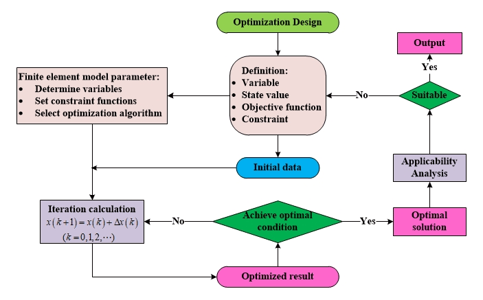
The establishment of the correct mathematical model is the key of the optimal design and the relevant parameters that are needed to discuss in the optimization process. The detailed process is given as follows:

1. determine the parameter type, initial value and variable range of the optimized design;

2. establish a parameterized model including design variables and solution parameters;

3. determine the objective function and its mathematical expression based on the optimization objective;

4. define the range of the rotor to ensure the movement range of the design point can be controlled within the feasible region;

5. check the rationality of the optimization design model to improve the efficiency and stability;

6. set the initial value, upper and lower bounds of the variables, optimize operating parameters, and complete computer programming.

3.1.1 Design variables

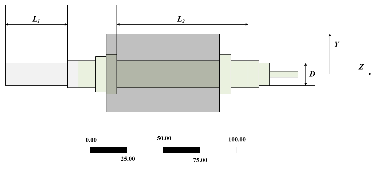
This paper uses $x_i(i=\mathrm{1},\mathrm{2},\mathrm{\dots },n)$ to present the deign variables, and they can be shown by a matrix as $x=[x_{\mathrm{1}},x_{\mathrm{2}},\mathrm{\dots },x_n{]}^{\mathrm{T}}$, where $x_{\mathrm{1}},x_{\mathrm{2}},\mathrm{\dots },x_n$ are n components of the vector x. And then Rⁿ is an n-dimensional European space, which can be generated by the design variables.

The function of the design variable is also called the state variable, which is used as the constraint of the design value. In this paper, the rotor mass (m), the first-order frequency (f_I) and the maximum stress (σ) are selected as state variables, which can be presented as follows:

$$\begin{array}{}\text{(29)}& y=[y_{\mathrm{1}},y_{\mathrm{2}},y_{\mathrm{3}}{]}^{\mathrm{T}}=[m,f_{\mathrm{I}},\mathit{\sigma }{]}^{\mathrm{T}}.\end{array}$$

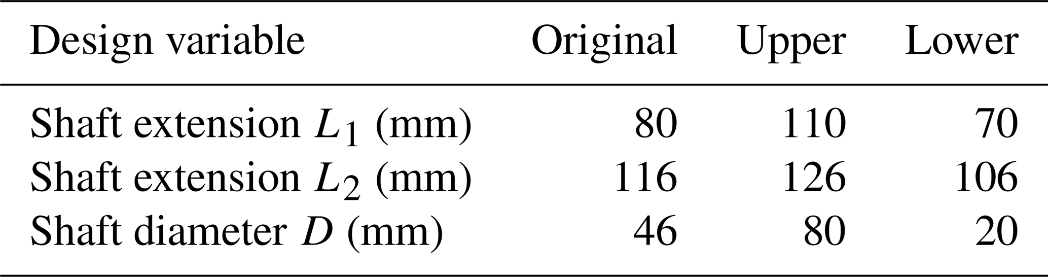
According to the definition, Fig. 3 shows the design variables including the shaft extension L₁, the shaft segment length L₂ and the shaft diameter D. Then the optimization design problem of the motor rotor can be seen as an optimization problem of mathematical model.

Figure 3 Design variables in the rotor optimization process.

3.1.2 Objective function

Objective function can be expressed as F(x). For the asynchronous motor, the rotor optimization design requires high rigidity and light mass, which can be recognized as multi-objective optimization problem:

$$\begin{array}{}\text{(30)}& \left\{\begin{array}{l}maxf\left(x\right)=maxf(x_{\mathrm{1}},x_{\mathrm{2}})\\ minm\left(x\right)=minm(x_{\mathrm{1}},x_{\mathrm{2}})\end{array}\right.\end{array}$$

• High rigidity. If the high rigidity of the asynchronous motor rotor is the objective function, the dynamic stiffness of the rotor should be increased as much as possible. Due to the inevitable error during the assembling process of the asynchronous motor, it can cause an imbalance that is dynamically affected by the mass. Therefore, the dynamic stiffness of the rotor must be sufficiently large. We describe the stiffness by the vibration amplitude of the rotor under dynamic excitation, and the dynamic stiffness (K) is $K=F_{\mathrm{e}}/A$, where F_e is dynamic excitation load and A is the corresponding displacement amplitude.

  In reality, the dynamic excitation of the rotor is constantly changing. When the changing frequency is far from the first natural frequency of the rotor, the dynamic stiffness and static stiffness are basically the same; when the changing frequency of the dynamic excitation is close to the first natural frequency of the rotor, the corresponding displacement amplitude will increase sharply and resonance will appear. Therefore, in order to achieve the high stiffness of the rotor, the first-order natural frequency of the rotor needed to be increased. So the relevant structural parameters will be changed, which make the first-order natural frequency and the dynamic stiffness increase simultaneously. Therefore, the high-stiffness problem can be transformed into the first-order frequency solution.

• Light mass. The mass of the rotor directly affects its dynamic unbalance state under high-speed operation. Therefore, it is required to reduce the rotor mass as much as possible. In this paper, the mass level is divided into higher, default and lower, which represents the priority and importance of the optimal solution. Therefore, the high-rigidity target is determined as the higher level, and the light mass is positioned at original level.

3.1.3 Constraint condition

Besides design variables and objective functions, constraint condition is required, and it can be generally divided into equality constraint (Eq. 31) and inequality constraint (Eq. 32).

$$\begin{array}{}\text{(31)}& g(x_{\mathrm{1}},x_{\mathrm{2}},\mathrm{\dots },x_n)=\mathrm{0}\end{array}$$

or

$$\begin{array}{}\text{(32)}& h(x_{\mathrm{1}},x_{\mathrm{2}},\mathrm{\dots },x_n)\ge h(x_{\mathrm{1}},x_{\mathrm{2}},\mathrm{\dots },x_n)\ge \mathrm{0},\end{array}$$

where g(x) and h(x) are the objective function with n-dimensional vectors. According to the above definition, the constraint condition in the optimization design of asynchronous motor rotor can be defined that the maximum stress of the shaft under the torque does not exceed the allowable stress of the shaft material:

$$\begin{array}{}\text{(33)}& \mathit{\sigma }(L_{\mathrm{1}},L_{\mathrm{2}},D)\le \left[\mathit{\sigma }\right].\end{array}$$

3.2 Optimization algorithms

In order to find the suitable parameters for the design of the asynchronous motor rotor, this section described a improved algorithm based on response surface optimization(RSO) and named it as accelerated response surface optimization (ARSO). Moreover, three algorithms – including traversal search algorithm (TS), multi-objective genetic algorithm (MOGA) and RSO – are chosen to evaluate the effectiveness of ARSO. The following sections mainly describe ARSO, but the other three algorithms (Fang and Xu, 2017; Ponnambalam et al., 2000; Munck et al., 2008) are also briefly described.

3.2.1 Accelerated optimization algorithm based on response surface (ARSO)

In order to improve poor generalization ability of traditional RSO (Ponnambalam et al., 2000), the least squares support vector machine (LS-SVM) provides a new way of structural reliability analysis (Deng et al., 2003; Cao et al., 2014) on RSO. Firstly, the inequality constraint function of SVM is converted into equality constraint function:

$$\begin{array}{}\text{(34)}& minJ(\mathit{\omega },e)={\displaystyle \frac{\mathrm{1}}{\mathrm{2}}}\Vert \mathit{\omega }{\Vert }^{\mathrm{2}}+{\displaystyle \frac{C}{\mathrm{2}}}\sum _{i=\mathrm{1}}^l{e}_i^{\mathrm{2}}.\end{array}$$

And constraint condition

$$\begin{array}{}\text{(35)}& y_i={\mathit{\omega }}^{\mathrm{T}}\mathit{\varphi }\left(x_i\right)+b+e_i,i=\mathrm{1},\mathrm{2},\mathrm{\dots },l,\end{array}$$

where ω is the weight vector, C is the penalty factor, e_i is the error, ϕ is the non-linear function of low-dimensional to high-dimensional mapping, and b is constant coefficient.

Then the squared error can be weighted to promote robustness:

$$\begin{array}{}\text{(36)}& minJ(\mathit{\omega },e)={\displaystyle \frac{\mathrm{1}}{\mathrm{2}}}\Vert \mathit{\omega }{\Vert }^{\mathrm{2}}+{\displaystyle \frac{C}{\mathrm{2}}}{v}_i\sum _{i=\mathrm{1}}^l{e}_i^{\mathrm{2}}.\end{array}$$

And constraint condition

$$\begin{array}{}\text{(37)}& y_i={\mathit{\omega }}^{\mathrm{T}}\mathit{\varphi }\left(x_i\right)+b+e_i,i=\mathrm{1},\mathrm{2},\mathrm{\dots },l,\end{array}$$

where v_i is the weight coefficient. Finally, the new regression prediction function can be obtained by Lagrangian polynomials:

$$\begin{array}{}\text{(38)}& y\left(x\right)=\sum _{i=\mathrm{1}}^l{\mathit{\alpha }}_{i}K(x,x_i)+b,\end{array}$$

where α_i is Lagrange multiplier, and K(x,x_i) is kernel function.

It is time-consuming based on the above calculation. The reason is when (K(x,x_i)) is used to construct shape functions, an n×n linear system should be computed for every computational point. If m monomials are added, an $(n+m)\times (n+m)$ linear system should be solved. Therefore, this paper proposes an accelerated optimization based on the previous works and name it ARSO.

For the LS-SVM based on RSO, kernel function includes [K^T(x)p^T(x)] and K⁻¹. The time consumption of [K^T(x)p^T(x)] is less than that of K⁻¹ because the computational complexities are o(n+m) and o((n+m)³), respectively. Every computational point has its own [K^T(x)p^T(x)] and is different from the rest, but it may have the same K⁻¹ as the other. Thus, we need a storage place, containing the public nodes and the corresponding points' information.

First of all, we construct an N_com×N_cor matrix S=[s_ij]. N_com×N_cor denotes the number of the computational nodes and the number of the corresponding points, respectively. The element S=[s_ij] is a δ function.

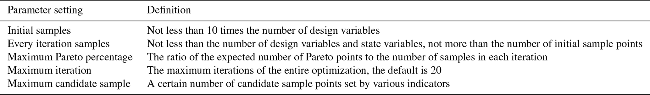
If the jth row elements are the same as the kth row elements, we confirm the jth and kth Gauss points have the same kernel functions K(x_j) K(x_k). It is a rule, which gives one-to-one mappings between the two type sets by comparing the rows of S. During the calculation process, the improved method can preset the search area to reduce the number of repeated matrix inversions. To ensure the algorithm's effectiveness, the main parameter settings are shown in Table 1.

Table 1 Main parameter settings.

3.2.2 Three compared algorithms

We select three traditional algorithms to compare. These are traversal search algorithm (TS), multi-objective genetic algorithm (MOGA) and optimization algorithm based on response surface (RSO). TS is to randomly generate a certain number of sample points according to the design space of the independent variable and calculate the generated sample points one by one. MOGA is an algorithm with the characteristics of global random searching and implicit parallel searching. It simulates the problem-solving process as the genetic evolution process of biological populations to find the optimal solution. RSO is an optimization method based on limited design space. Firstly, a polynomial method is used to fit a response surface that is shown in Fig. 4; it is the response surface fitted by the quadratic polynomial. Secondly, all the points on the response surface form a subset of the design space, which reduces the design space of the entire optimized design and improves the computational efficiency.

Figure 4 Response surface fitted by a quadratic polynomial.

3.3 Optimization processing

3.3.1 Optimal solution

The optimization design problem includes establishing the model and solving the model. Solving the model is to obtain the optimal solution. The next step is to analyze and judge the practicality of the optimal solution and finally determine the optimal design plan.

Generally, the n design variables can make the objective function reach the extreme value under the restriction of constraints:

$$\begin{array}{}\text{(39)}& \left\{\begin{array}{ll}minf\left(x\right)=f\left(x^{*}\right),& x\in X\subset R^n\\ s.t.g_u\left(x^{*}\right)\le \mathrm{0},& u=\mathrm{1},\mathrm{2},\mathrm{\dots },m\\ h_v\left(x^{*}\right)\le \mathrm{0},& v=\mathrm{1},\mathrm{2},\mathrm{\dots },p.\end{array}\right.\end{array}$$

When the constraint function is a non-convex set or the objective function is a non-convex function, there may be multiple optimal solutions. The optimal solution obtained is called a local optimal solution. Only when the set of constraints is a convex set or the objective function is a unimodal function in the domain can the obtained local optimal solution be judged as the global optimal solution.

3.3.2 Modify the original model parameters

Once the final optimization plan is determined, the original model can be modified according to the parameter values of the optimal solution, which could improve product performance and reduce manufacturing costs.

3.3.3 Simulation analysis of optimization scheme

During the initial establishment of the optimal design model, due to the complexity of the actual problem and the limitations of the mathematical model description, some design parameters and constraints were simplified. After the final optimization plan is determined, the simplified content should be added to the fractional finite element model again, and then the static and dynamic characteristics that are closer to the actual geometric model can be simulated.

4 Experimental results

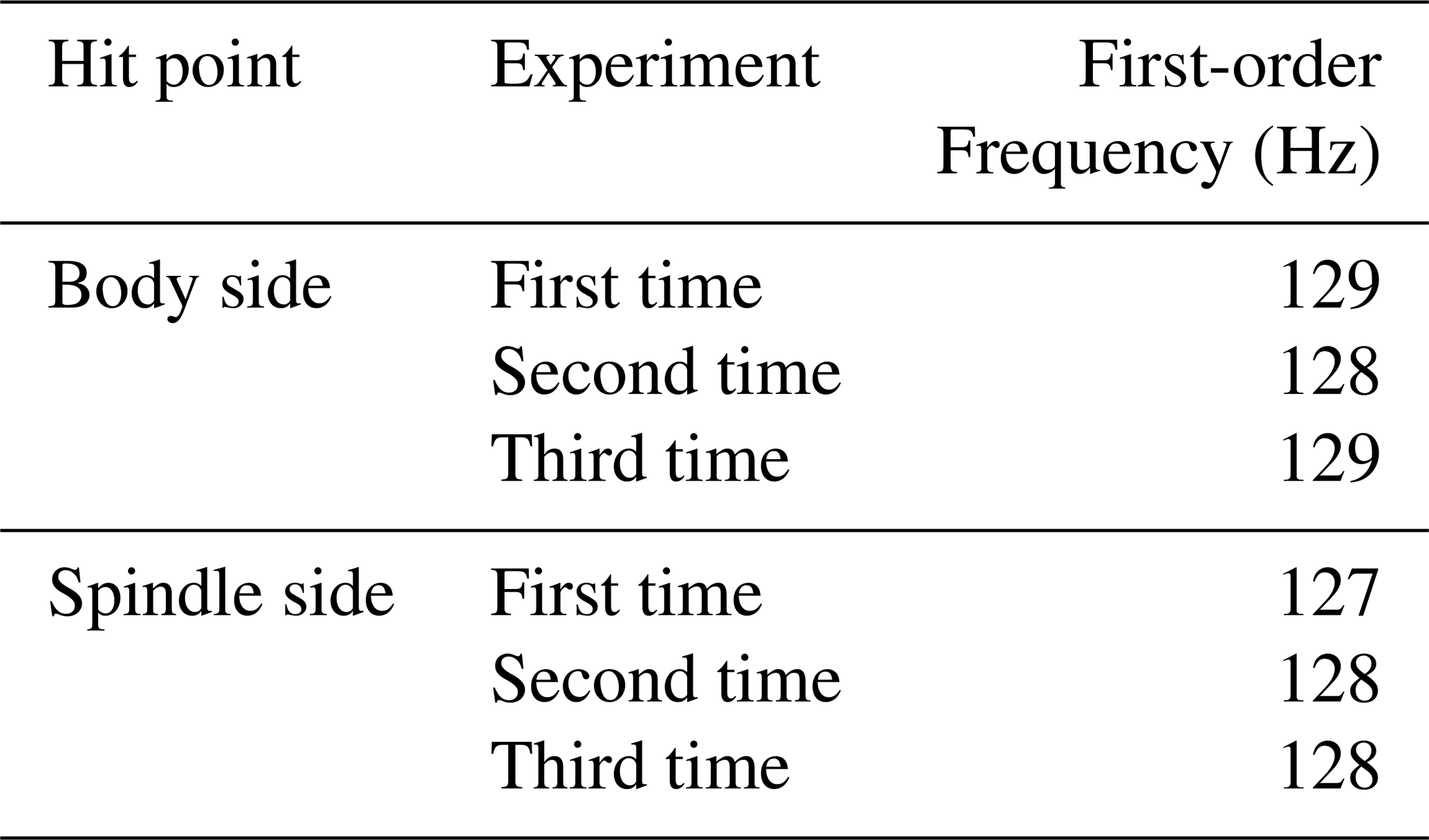
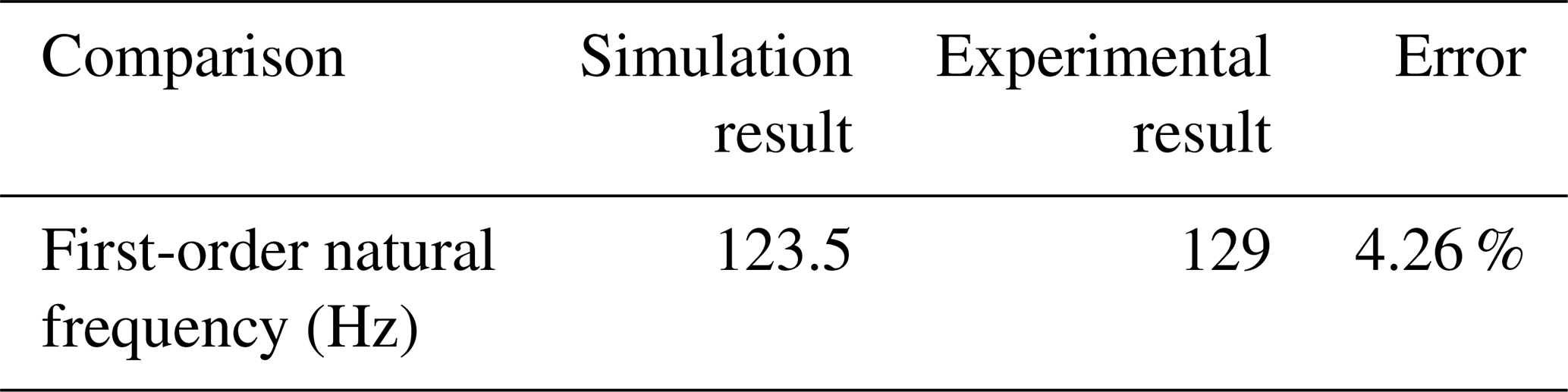
In order to verify the correctness of the established fractional model, it is necessary to explore whether its dynamic response is consistent with the actual asynchronous motor. Therefore, a modal test of the asynchronous motor percussion method is designed to measure the natural frequency of the asynchronous motor in a free state. In the experiment, the asynchronous motor was suspended with a flexible rope to make it in a free state. The experimental instrument relied on the German Plufor vibration analyzer Vib Xpert-II. By pasting an acceleration sensor on one side of the GM7101 motor, it was hit with a hammer on the opposite side. The vibration response of the asynchronous motor can be measured by the hammering experiment module in Vib Xpert-II. The suspension mode and sensor arrangement of asynchronous motor are used in The State Key Laboratory of Automotive Simulation and Control (ASCL). The GM7101 test site is shown in Fig. 5. Then the modal test results are given in Table 2, and the comparison between simulation results and experimental results is given in Table 3.

Figure 5 GM7101 motor test site.

Table 2 Modal test results.

In Table 3, it can be seen that the first-order frequency obtained by the simulation calculation is slightly lower than the experimental results, and the error may be caused by the following:

1. When the three-dimensional model and finite element model are established, many simplified principles are adopted, and many small chamfers, threads, ventilation ducts and other structures are ignored.

2. The influence of contact stiffness and damping factors of the contact surface is ignored.

3. Silicon steel entities are used to bringing inevitable errors.

4. The actual bearing has a clearance. The clearance of the bearing is ignored when the spring structure is used for equivalent replacement, which causes a deviation in the modal analysis.

5. The experimental instrument and its installation may bring a few errors.

6. The boundary condition of the simulation analysis is a completely free state, but the suspension method used in the experiment is not easy to achieve the completely free state.

Table 3 Comparison between simulation results and experimental results.

5 Optimization analysis

This section introduces the optimized settings and analyzes the optimal results.

5.1 Optimization settings

5.1.1 Design variables

As shown in Table 4, three design variables are defined respectively: the shaft extension L₁, the shaft segment length L₂ and the shaft diameter D.

Table 4 Range of design variables.

5.1.2 State variables

There are three state variables for the rotor optimization design problem of asynchronous motors: the mass of the rotor m, the first-order natural frequency f₁ and the maximum stress σ.

5.1.3 Constraint conditions

The maximum bending stress does not exceed the allowable shear stress, which is σ≤50 MPa.

5.1.4 Objective function

The main goal of the rotor optimization design of the asynchronous motor is to improve the high rigidity of the rotor but to minimize the rotor mass. Therefore, there are two objective functions: the first-order natural frequency of the rotor should be as large as possible when it exceeds the frequency corresponding to the maximum speed; the rotor mass is as small as possible under 10 % reduction of the mass. The relevant settings of state variables, constraint conditions and objective function are described in Table 5.

Figure 6 The curve of the harmonic response model.

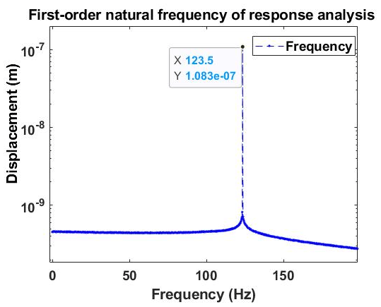
Table 5 Settings of state variables, constraints and functions.

Table 6 Calculation results of the four algorithms.

Figure 7 Relationship between objective function and design variables.

5.2 Optimization results

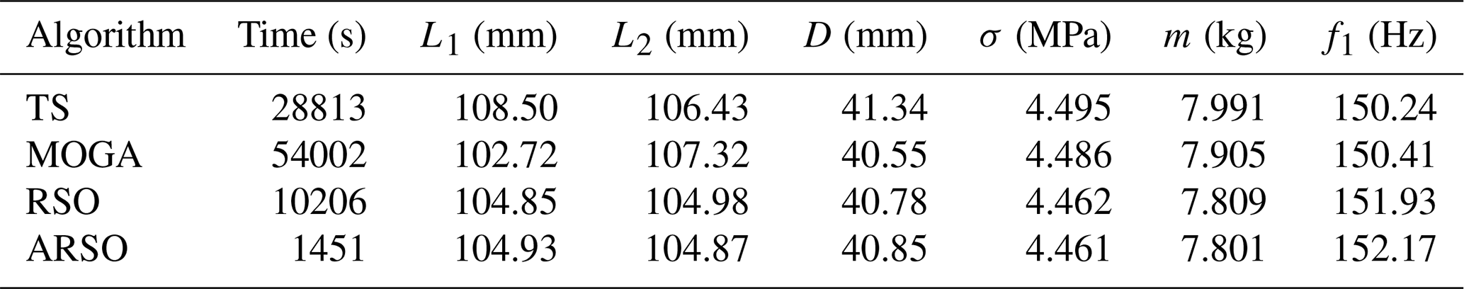
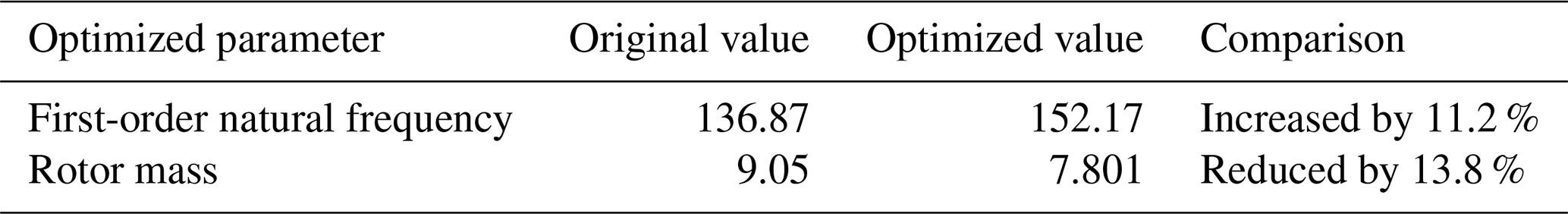
As seen in Table 6, it can be found that the optimization results obtained by the four algorithms are all acceptable. The first-order natural frequencies obtained by TS and MOGA are both around 150.4 Hz, which is smaller than 152 Hz, which was obtained by the RSO and ARSO. Meanwhile, there are no large differences in the mass obtained by the four algorithms, but the calculation time of ARSO is the least compared to the other three algorithms. On the whole, the proposed ARSO performs better than other algorithms, and the first-order natural frequency and the lightest mass are 152.17 Hz and 7.801 kg, respectively.

Table 7 The rounding results of the optimal solution.

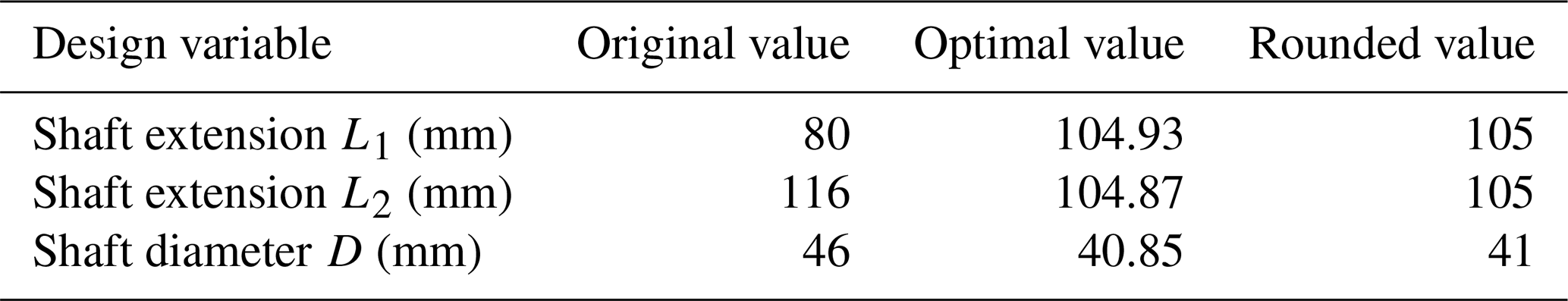
Table 8 Comparison of previous parameters and optimized parameters.

6 Discussion

6.1 Model validation

According to Eq. (28), modal superposition method is used to discuss the harmonic response and obtain the modal solution and mode shape. The frequency range is set to be 0–200 Hz, and the number of operations is 500; that is, the interval of each solution is 0.5 Hz. And the simple harmonic exciting force is added to two vertical directions of the shaft section on the shaft flywheel rotor. The amplitude is 0.001 N, and the phase is 0 and 90^∘.

The flying wheel is selected as the response surface, and the maximum displacement response is set as the vertical coordinate and the excitation frequency is set as the horizontal coordinate. As seen in Fig. 6, the harmonic response simulation curve is obtained. By analyzing the displacement response frequency curve, the peak can be found at 123.5 Hz, which is also the distribution position of the first two natural frequencies of the system. At this time, the system resonates and the response increases sharply, which fulfill the dynamic characteristics of the system and also prove the accuracy of the natural frequency calculation. Meanwhile, it can also be seen that the system has a greater vibration response when the rotor is operating in the first-order natural frequency range. After the harmonic response curve crosses the first-order natural frequency, it shows a downward trend with the increase of the exciting force frequency; that is, the disturbance vibration caused by the unbalanced force attenuates with the increase of the frequency. Then, the system enters the normal working range, and its stability is gradually improved. Moreover, the peak value of the displacement response of the shafting rotor is about 10⁻⁷ and extremely small. It indicates that the shafting is running well and there will be no collision between the bearing rotor and the stator.

According to the test results of 129 Hz in Tables 2 and 3, it can known that the response curve can effectively represent the real frequency distribution, especially the first natural frequency.

6.2 Design variables discussion

In the optimal phase, it is necessary to choose suitable design variables. This section discusses the relationship among those variables and obtains the optimal values.

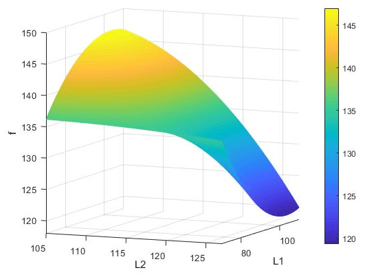
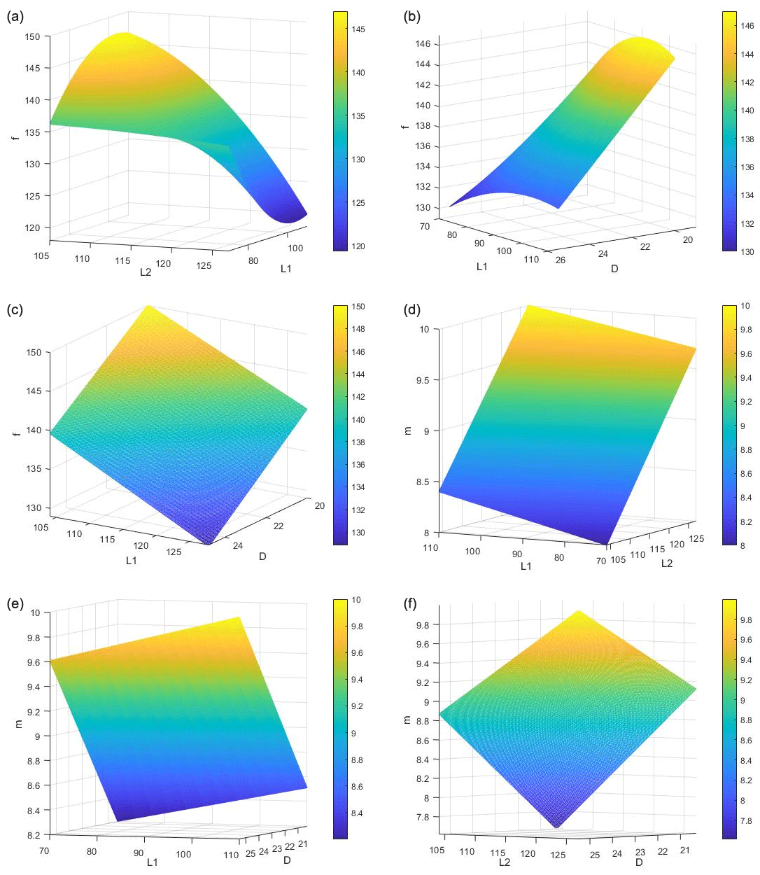
According to the relationship diagram shown in Fig. 7, the first three sub-features show that L₁ and L₂ are not linear with frequency especially for L₁. On the contrary, it can be found that natural frequency is linear with diameter in the third sub-figure, where it is consistent with the theoretical analysis. It is obvious that there is always a linear relationship between mass and length (L₁ or L₂) from the last three pictures.

In Table 7, the optimal solution is rounded by being combined with the rationality requirements of the actual structure of the rotor. The L₁ and L₂ are close to each other when the shaft diameter becomes smaller. The numerical results show that the longer the rotor length is, the higher the natural frequency is. In terms of mass, a smaller diameter can not only reduce the quality because the mass is proportional to the square of diameter, but also effectively offset the influence of length.

According to the above discussion, Table 8 gives the comparison between the original values and the optimized results. It can be seen that the first-order natural frequency is increased by 11.2 %, and the rotor mass is reduced by 13.8 %.

7 Conclusions

In this paper, the fractional model of the asynchronous motor rotor was firstly established with a peculiar memory characteristic, and the introduced harmonic response was able to fit the reality well. Then, we set high rigidity and less mass as optimization functions and transform them into the problem of the first-order frequency and mass. In order to find the optimal parameters, an accelerated optimization method based on response surface is proposed. Finally, the GM7101 asynchronous motor was selected to evaluate our work. The experimental results show that the optimized first-order natural frequency was increased by 11.2 %, and the mass was reduced by 13.8 %, where they verified the effectiveness and correctness of the fractional order and harmonic response analysis and realized the high rigidity and light mass of the asynchronous motor rotor.

However, an asynchronous motor is a complex system, and there are many factors that affect its vibration characteristics, such as frame type, ribs, ventilation ducts and so on. To study more complex asynchronous motors, more influencing factors will be considered in the future.