Analysis and control of state jump in space deployable structures under alternating temperature loads

State jump has been experimentally observed in space deployable structures working in alternating temperature environments. State jump is a phenomenon in which the geometric shape of the structure changes after the temperature loading and unloading process, which makes the working accuracy of the space deployable structure intrinsically unpredictable. This paper aims to investigate the causes of this state jump phenomenon and seek measures to reduce its effect. Firstly, the static multiple-stable-state phenomenon resulting in state jump is analyzed for clearance joints in deployable structures. Then, an equivalent model consisting of a variable stiffness spring and a contact element for state jump analysis is proposed, which is verified by a finite element simulation. Influence factors and control methods of state jump are further explored. Finally, numerical results of a space deployable structure of an umbrella-shaped antenna show the effectiveness of the developed analytical method.

1 Introduction

As the carrier of receiving and reflecting electromagnetic signals, the satellite antenna is a key piece of equipment for deep space explorations, satellite navigation, satellite communications and electronic reconnaissance. In order to achieve the ability of long-distance information transmission and capture weak signals, the satellite antenna is required to have a large aperture (Alfred and Joseph, 1998; Arnol and Naderi, 1989; Rahmat-Samii and Densmore, 2015). At the same time, due to the limitation of launch capability and space, large satellite antennas must be light and deployable. For this reason, space deployable structures have been widely used in constructing large satellite antennas.

The space deployable structure (Gantes, 2001) is a special kind of deployable mechanism, which can transform from a folding configuration with a small volume to a stable load-bearing structure configuration with a large volume or surface area. It is found in the ground test that even if temperature loads applied on space structures are identical, the structural state is inconsistent. Moreover, affected by solar radiation and earth shadow, space temperature is alternating from −180 to 150 ^∘C (Hu et al., 2013). These reasons make the working accuracy of space deployable structures intrinsically unpredictable.

So far, researches about space deployable structures under temperature loads are mainly focused on analysis and control of thermal deformations and thermally induced vibrations. For example, Tang et al. (2014) studied thermal deformation and surface accuracy of large deployable antennas in orbit based on the stochastic finite element method. Lu et al. (2019) studied thermal deformation and the shape adjustment method of a planar-phased array antenna structure. Thornton and Kim (1993) studied thermally induced vibrations of the cantilever beam of the Hubble Space Telescope and established the stability criterion of thermally induced vibrations. Shen et al. (2013) established thermal-structural analysis model of flexible beams using the absolute nodal coordinate formulation and studied its thermally induced vibrations. Azadi et al. (2017) studied thermally induced vibrations of smart solar panels and analyzed the influence of heat radiation and orbit parameters on the amplitude of thermal vibrations. Fazelzadeh and Azadi (2017) modeled the orbiting smart satellite panels as a functionally graded material beam and studied the control strategy of thermally induced vibrations.

While most of the above studies are mainly based on ideal structures, some other studies have shown that the thermal response of the structure is strongly affected by joint clearances in structure, which is inevitable in space deployable structures due to manufacturing errors and assembly requirements. Kim et al. (1999) studied the thermal-creak-induced dynamics caused by external temperature changes of space structures with clearances, but the influence of temperature changes on position accuracy and stability of the structure is not considered. With the urgent need for high-accuracy space deployable structures, the influence of clearance on the accuracy and stability of deployable structures cannot be neglected. To fill this research gap and meet the needs of high-precision and high-stability deployable structures in aerospace industry, further study of the state jump phenomenon is needed for space deployable structures with clearance joints.

This paper is organized as follows: first, kinematic joints of space deployable structures are classified and the static multiple-stable-state phenomenon in clearance joints is analyzed in Sect. 2. Then, the state jump analysis model is established and verified, and interfering factors and control methods of the state jump phenomenon are studied in Sect. 3. In Sect. 4, the above contents are verified by an example of an umbrella antenna. And conclusions are summarized in Sect. 5.

2 Static multiple-stable-state phenomenon in clearance joints

2.1 Classification of clearance joints

Ideally, the degree of freedom of a deployable structure is 0 when it is in deployment state. However, the existence of clearances in kinematic joints makes the structure movable to some extent.

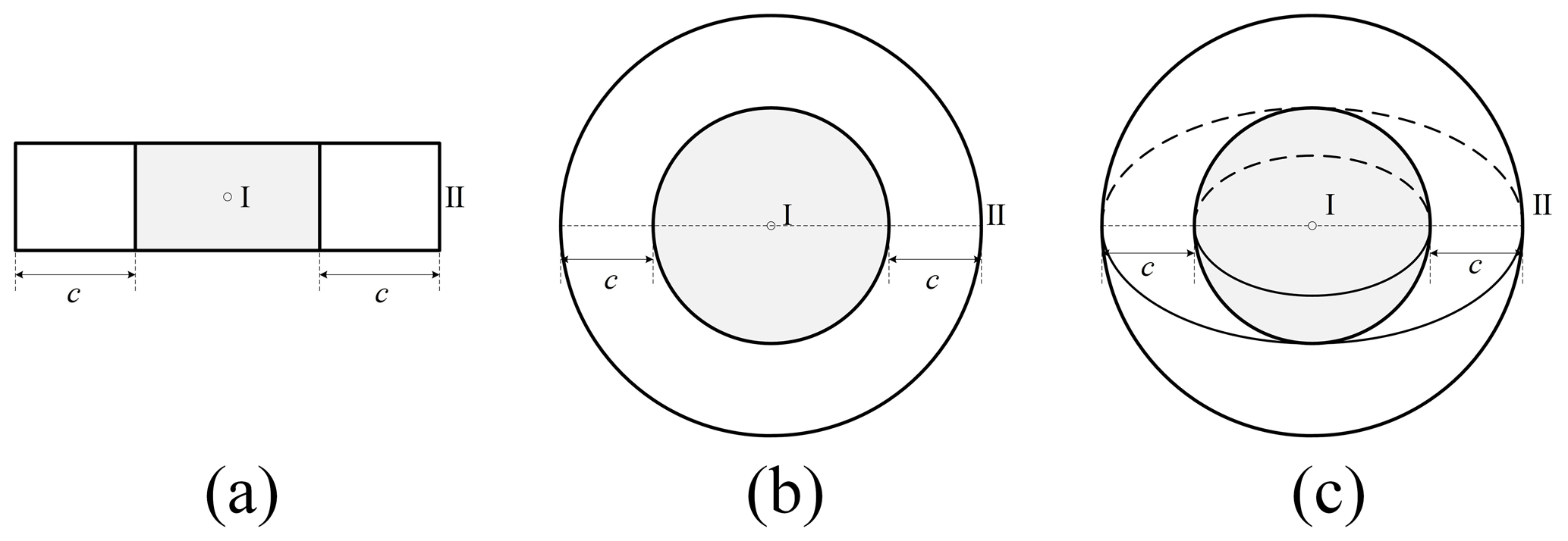
Kinematic joints in space deployable structures are divided into three types: one-dimensional clearance joint, two-dimensional clearance joint and three-dimensional clearance joint. The one-dimensional, two-dimensional and three-dimensional clearance joints allows small linear relative displacement, small planar displacement and small spatial relative displacement between the two components connected by the joint, respectively. Figure 1 shows these three types of clearance joints, in which I and II are two components connected by the clearance joint, and c is the size of the clearance. For illustration, the clearance in Fig. 1 is enlarged.

Figure 1 Classification of clearance joints.

2.2 Static multiple-stable-state phenomenon

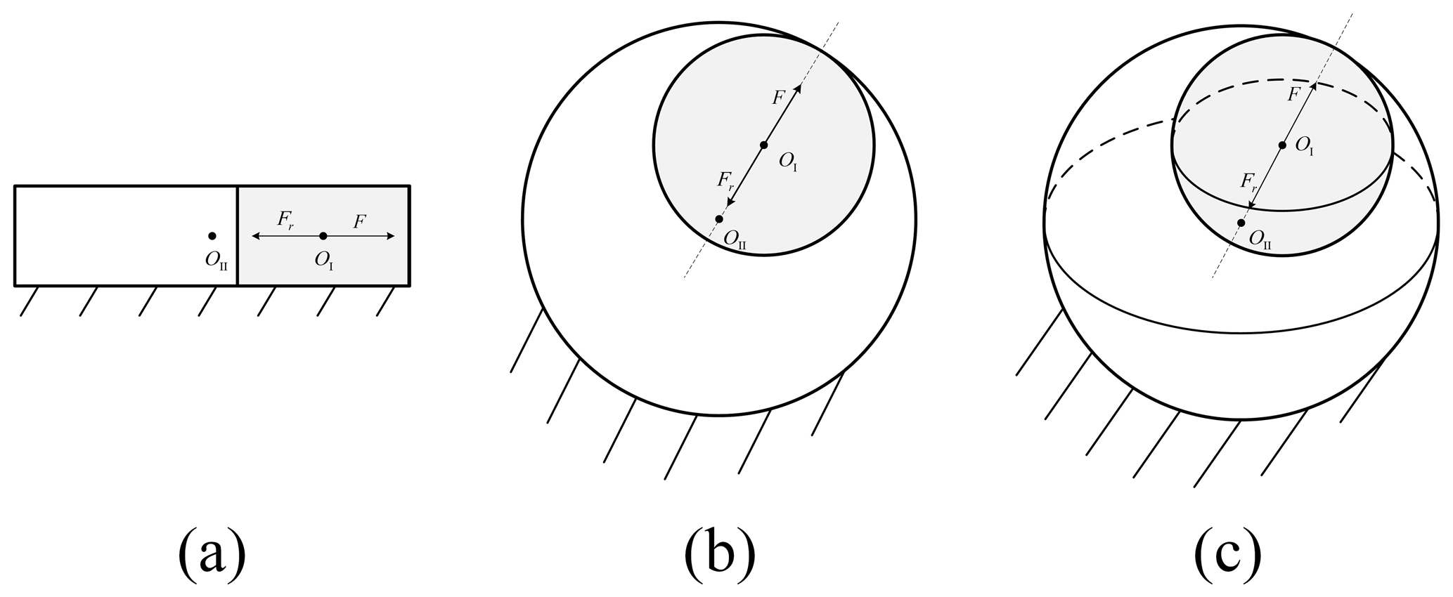
Without losing the generality, it is assumed that the pairing element of component II is a second-order continuous surface $S=\mathrm{\Gamma }\left(x,y,z\right)$. When component II is fixed and a spatial external force $\mathit{F}=(F_x,F_y,F_z)$ at the centroid of component I is applied, component I will eventually be balanced under the combined action of the external force F and reaction force F_r provided by component II, that is

$$\begin{array}{}\text{(1)}& \mathit{F}+{\mathit{F}}_{\mathrm{r}}=\mathit{F}+{\mathit{F}}_{\mathrm{N}}+{\mathit{F}}_{\mathrm{T}}=\mathbf{0},\end{array}$$

where F_N, F_T are normal and tangential components of reaction force F_r, respectively. According to the force equilibrium condition, F_N, F_T and F are coplanar.

For an arbitrary point $(x,y,z)$ on S, Eq. (1) has an exclusive resolution (F_N0,F_T0). If and only if F_N is positive (pointing from the component II to the component I) and |F_T|≤μ|F_N|, the component I can be balanced at this point, where μ is the friction coefficient of the contact surface. When the above conditions are not satisfied, component I cannot be balanced at this point.

By solving Eq. (1), the following can be found:

1. When there is no friction in the clearance joint (μ=0), component I under a given external force F can be balanced at only one point, as shown in Fig. 2. O_I and O_II are the centers of component I and component II, respectively.

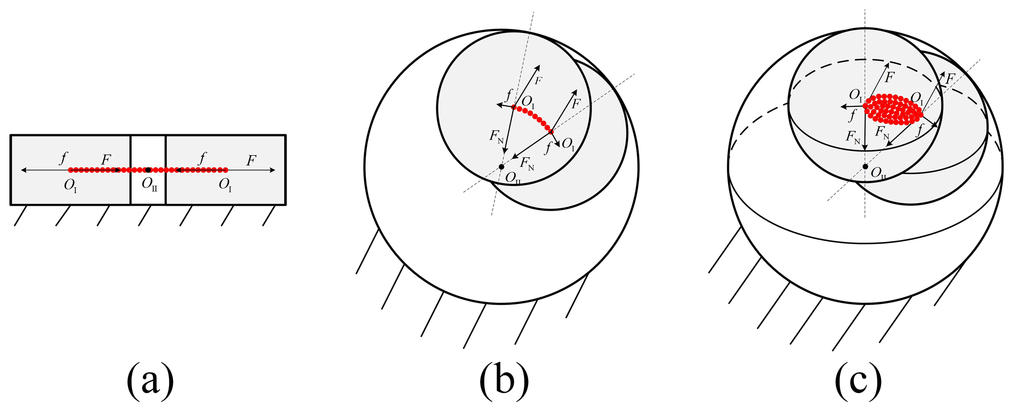
2. When μ≠0, component I could be balanced in multiple positions, as shown in Fig. 3. The filled circles in Fig. 3 represent possible equilibrium positions of component I. For two components connected by a one-dimensional, two-dimensional or three-dimensional clearance joint, their relative equilibrium positions can be expressed as a straight line, a spatial curve or a spatial surface, respectively.

In summary, due to the existence of clearance and friction in deployable structure joints, the static equilibrium position of space deployable structure components under external force is not unique. In other words, there is a static multiple-stable-state phenomenon. This phenomenon makes the state jump occur in space deployable structures.

Figure 2 Static equilibrium position of frictionless clearance joints.

Figure 3 Static equilibrium positions of friction clearance joints.

3 State jump phenomenon in clearance joints

3.1 Analysis model of the state jump phenomenon

The analysis model of deployable structure component used in this paper is shown in Fig. 4. The structure component is composed of a massless spring and a lumped mass block, and it may deform axially under the temperature loads. In order to distinguish intrinsic factors related to the state jump phenomenon, the quasi-static assumption is introduced; that is, the accumulation and release of elastic energy in the component is instantly completed.

When the temperature change is ΔT, the length change of the component is

$$\begin{array}{}\text{(2)}& \mathrm{\Delta }l={\mathit{\alpha }}_{\mathrm{L}}\mathrm{\Delta }T\cdot l,\end{array}$$

where Δl, l and α_L denote the thermal deformation, original length and coefficient of linear thermal expansion of the component, respectively.

Figure 4 State jump analysis model.

According to the Hooke's law, the relationship between the axial force and the section stress σ and deformation Δl of the flexible member is

$$\begin{array}{}\text{(3)}& F=\mathit{\sigma }A={\displaystyle \frac{EA}{l}}\mathrm{\Delta }l,\end{array}$$

where E and A are the elastic modulus and cross-sectional area of the component, respectively.

When the axial force in the component is insufficient to overcome the maximum friction force provided by the contact surface, the length of the component will remain the same and the energy of the external temperature load will be accumulated in the form of elastic energy. If the difference between the actual deformation and thermal deformation of the component is Δx, the axial force in the component can be calculated as

$$\begin{array}{}\text{(4)}& F={\displaystyle \frac{EA}{l_t}}\mathrm{\Delta }x=k_t\mathrm{\Delta }x,\end{array}$$

where l_t is the stress-free length of the component at time t. Therefore, the non-linear spring is used to establish the equivalent mechanical model of the structure component.

3.2 State jump analysis

The temperature applied on the structure is assumed to be T₀ at the beginning, and after a certain loading process, the temperature returns to T₀ for the first time.

When there is no friction in the clearance joint and the clearance size is large enough, the component will expand and contract freely under external temperature loads. When the temperatures before and after loading are the same, the structural states will also be the same; in other words, the lumped mass block will return to its original position at the end of the loading process.

When there is no friction in the clearance joint and the clearance size is small, elastic energy will be accumulated in the component when the length variation of the component caused by temperature is greater than the clearance size. Once the temperature changes inversely, the energy accumulated in the component will be released, and there is no energy dissipation in the process when the complete elastic deformation is considered. Therefore, the lumped mass block will still return to its original position after unloading.

When there is friction in the clearance joint, energy dissipation and transfer will occur during the loading process, which makes it impossible for the lumped mass block to return to its original position. There exists the state jump phenomenon.

As shown in Fig. 5, when the clearance size is large enough, the system will go through five typical stages. In the figure, x_t and x_T are actual displacement (deformation) and theoretical thermal displacement (deformation) of the component, respectively.

Figure 5 Typical thermal loading process.

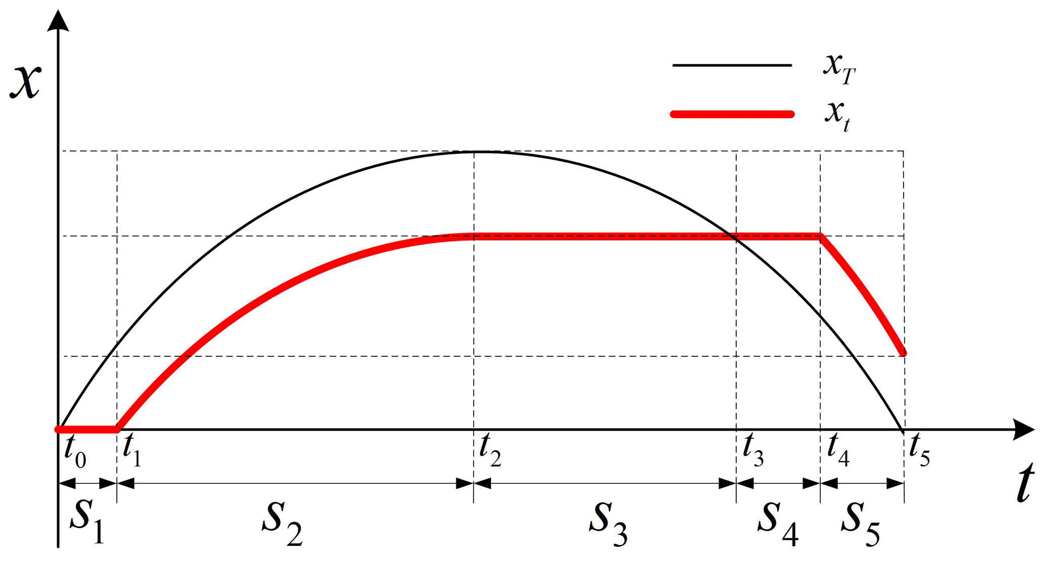
3.2.1 Stage S₁: static stage 1

In this stage, the stress caused by temperature change is not enough to overcome the friction force, and the actual length of the component remains unchanged. The component is subjected to an axial force F_t(|F_t|≤f), where f is the maximum static friction provided by the contact surface. The actual deformation of the component in this stage is x_t=0.

3.2.2 Stage S₂: sliding stage 1

In this stage, the insufficient friction cannot keep the component maintaining its current length, and the component begins to deform. The axial force in the component is |F_t|=f. The actual deformation of the component is $x_t=x_{\mathrm{T}}-\mathrm{sign}\left(\frac{\mathrm{d}{x}_{\mathrm{T}}}{\mathrm{d}t}\right)\frac{l_{t}f}{EA}$, where sign(A) is the sign function.

3.2.3 Stage S₃: static stage 2

In this stage, the external environment temperature begins to change reversely, and the elastic energy stored in the component is released. The axial force in the component is |F_t|≤f. The actual deformation of the component in this stage is $x_t=x_{t_{\mathrm{2}}}$.

3.2.4 Stage S₄: static stage 3

Similar to S₁, in this stage, the actual length of the component remains unchanged, and the axial force in the component is |F_t|≤f. The actual deformation of the component in this stage is $x_t=x_{t_{\mathrm{2}}}$.

3.2.5 Stage S₅: sliding stage 2

Similar to S₂, the friction is insufficient and the component begins to deform reversely. The axial force in the component is |F_t|=f. The actual deformation of component I is $x_t=x_{\mathrm{T}}+\mathrm{sign}\left(\frac{\mathrm{d}{x}_{\mathrm{T}}}{\mathrm{d}t}\right)\frac{l_{t}f}{EA}$.

3.3 Validation of the analysis model

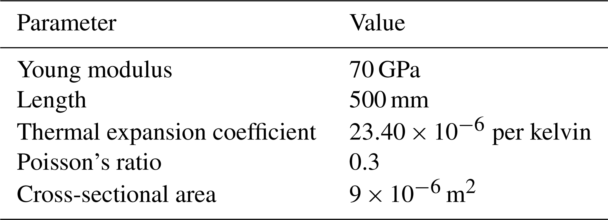
Geometric and material parameters of component I are shown in Table 1, and the friction force is 30 N. The state jump value Det can be calculate as $\mathrm{Det}=\frac{l_{t}f}{EA}=\frac{\mathrm{0.5}\times \mathrm{30}}{{\mathrm{70}}^{\mathrm{9}}\times {\mathrm{9}}^{-\mathrm{6}}}\times \mathrm{1000}\mathrm{mm}=\mathrm{0.024}\mathrm{mm}$, as discussed in Sect. 3.2.

Table 1 Geometric and material parameters of component I.

The finite element simulation model is established and analyzed using the ANSYS software to verify the effectiveness of the above analysis model. As shown in Fig. 6, a BEAM188 element and a SOLID185 element are chosen to simulate component I and component II, respectively. The contact pairs between the lower surface of component I and the upper surface of component II are established using a CONTA170 element and a TARGET169 element, respectively. Two CONTA178 elements with an initial gap size of c are used to simulate the horizontal contact between the components. A vertical force F_n is applied to keep the components in contact state.

Figure 6 Schematic diagram of finite element model.

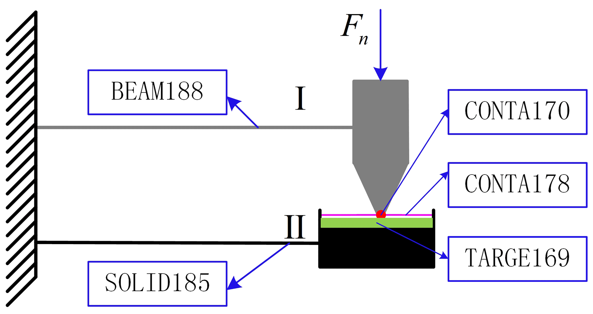
In the simulation, component II is regarded as the grid, the clearance size is 1 mm, the friction coefficient between the components is 0.3, the vertical force is −100 N (the corresponding friction is 30 N), the variation of the environmental temperature is 100 K and the temperature changes in a sinusoidal law.

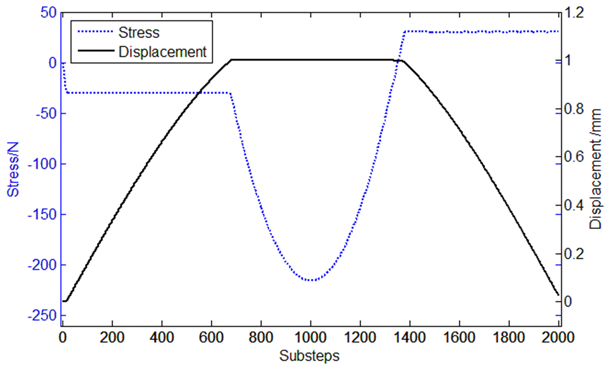
The displacement and force curves of component I by simulation analysis are shown in Fig. 7.

Figure 7 Displacement curve of component I.

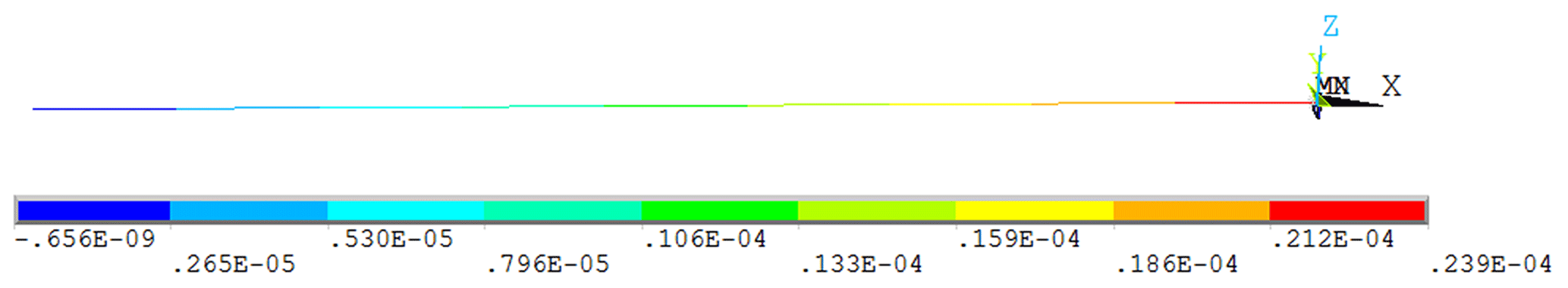
The color cloud picture of displacement of component I is shown in Fig. 8. The maximum deformation at the right of the component is 0.0244 mm, which is consistent with the result of the equivalent analysis model.

Figure 8 Color cloud picture of displacement.

3.4 Control of the state jump phenomenon

It can be seen from Sect. 3.2 that, for two components connected by a one-dimensional clearance joint, the deformation of the component after being loaded is $\frac{l_{t}f}{EA}$, which means the state jump value is independent of the motion path of the component. The main factors affecting the state jump value are the magnitude of friction and the axial stiffness of the component, while the maximum thermal deformation and clearance mainly affect the shape of the structure during the temperature loading process. Therefore, the following measures may be taken to control the state jump phenomenon.

1. Control the friction between components. The main factors affecting the friction between components are the contact pressure, friction type, material type and roughness of the contact surface. Therefore, the control of the state jump phenomenon can be realized by choosing and controlling component materials, processing technology and components matching types.

2. Control the deformation stiffness of components. The main factor affecting the deformation stiffness of components is the material of the component. Besides, the deformation stiffness of the component can also be increased by setting preload springs in the clearance joint. Therefore, the control of the state jump phenomenon can be realized by reasonably selecting the materials of the components and adding preload springs in kinematic joints.

The following should be noted:

1. Applications of above control measures may affect the deployment process or other performances of the structure, which should be considered comprehensively.

2. With the increase in the dimension and number of clearance joints, the affecting factors may be different and the control of the state jump phenomenon may become much more complicated.

4 Simulation analysis

4.1 Modeling of deployable structure of umbrella antenna

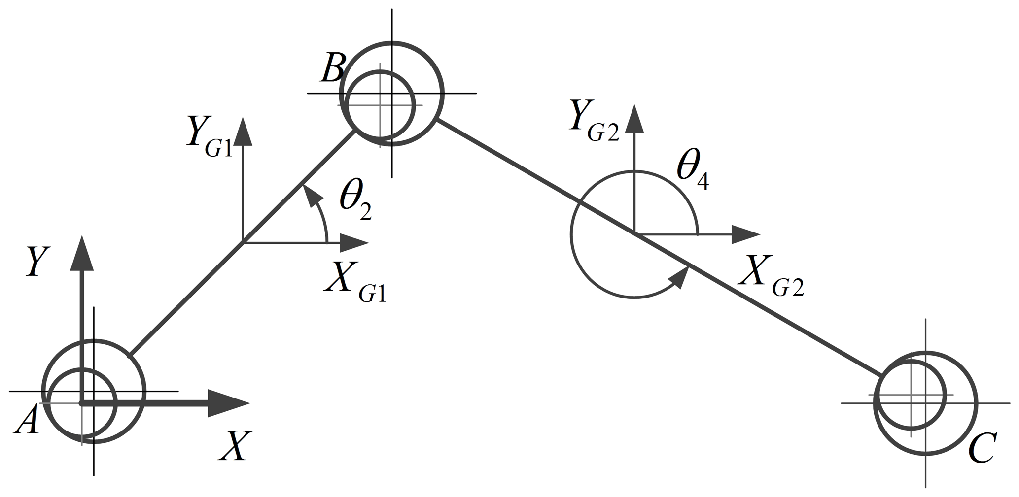
The equivalent modeling method proposed in Sect. 3 is used to analyze the deployable structure of an umbrella-shaped antenna. The deployment principle of the umbrella-shaped deployable antenna is shown in Fig. 9. The motor drives the slider D to move to realize the closure and expansion of the antenna.

Figure 9 Deployment principle of umbrella antenna.

In Fig. 9, link AB is fixed to the antenna rib, A is a joint at the root of antenna rib, B is located at an eccentric position of the rib root, BC is the connecting rod and CD is the sliding disk. The dotted line in Fig. 9 represents the folded state of the antenna while the solid line represents the unfolded state. After being deployed and locked in place, the mechanism degenerates into a structure and AC is equivalent to the frame. The equivalent deployable structure is shown in Fig. 10. X_G1, Y_G1, X_G2 and Y_G2 are the centroid coordinates of links AB and BC. θ₂ and θ₄ are the angles between the links and the horizontal direction.

Figure 10 Deployable structure with clearance joints.

Dynamic equations of the structure are established using the Lagrange method,

$$\begin{array}{}\text{(5)}& {\displaystyle \frac{\mathrm{d}}{\mathrm{d}t}}\left({\displaystyle \frac{\partial (T-V)}{\partial q_j}}\right)-{\displaystyle \frac{\partial (T-V)}{\partial q_j}}=Q_j(j=\mathrm{1},\mathrm{2},\mathrm{\dots },\mathrm{6}),\end{array}$$

where $q=(X_{\mathrm{G}\mathrm{1}},Y_{\mathrm{G}\mathrm{1}},X_{\mathrm{G}\mathrm{2}},Y_{\mathrm{G}\mathrm{2}},{\mathit{\theta }}_{\mathrm{2}},{\mathit{\theta }}_{\mathrm{4}})$ denotes the generalized coordinates, T is the kinetic energy, V is the potential energy of the system and Q_j is the generalized force corresponding to q_j. The generalized force Q_j is a function of contact forces and friction forces in clearance joints. The classical Hertz contact force model (Lankarani and Nikravesh, 1990) and Ambrósio friction model (Ambrósio, 2003) are introduced to calculate Q_j.

The classical Hertz contact force model is

$$\begin{array}{}\text{(6)}& {\displaystyle }{F}_{\mathrm{N}}=K{\mathit{\delta }}^n,\text{(7)}& {\displaystyle }K={\displaystyle \frac{\mathrm{4}}{\mathrm{3}\mathit{\pi }\left(h_{\mathrm{1}}+h_{\mathrm{2}}\right)}}{\left({\displaystyle \frac{R_{\mathrm{1}}{R}_{\mathrm{2}}}{R_{\mathrm{1}}+R_{\mathrm{2}}}}\right)}^{\mathrm{1}/\mathrm{2}},\text{(8)}& {\displaystyle }{h}_{\mathrm{1}}={\displaystyle \frac{\mathrm{1}-{\mathit{\rho }}_{\mathrm{1}}^{\mathrm{2}}}{\mathit{\pi }{E}_{\mathrm{1}}}},h_{\mathrm{2}}={\displaystyle \frac{\mathrm{1}-{\mathit{\rho }}_{\mathrm{2}}^{\mathrm{2}}}{\mathit{\pi }{E}_{\mathrm{2}}}},\end{array}$$

where K is the stiffness coefficient, δ is the penetration depth, and n is the force index which depends on material and geometric properties. For metal contact, n is generally 1.5. R₁ and R₂ are the radii of two contact bodies, and the material coefficient h_i depends on Young's modulus E_i and Poisson's ratio ρ_i of the contact body.

The Coulomb friction model is the most classical friction model but it does not take the tangential velocity between the two contact components into account. When the tangential velocity is in the vicinity of zero, the value of friction force is changed from F_t to −F_t, leading to numerical solving difficulties. To address these problems, Ambrósio proposed a modified Coulomb friction model (Ambrósio, 2003):

$$\begin{array}{}\text{(9)}& {\displaystyle }{F}_{\mathrm{T}}={\mathit{\mu }}_{\mathrm{f}}{\mathit{\mu }}_{\mathrm{d}}{F}_{\mathrm{N}},\text{(10)}& {\displaystyle }{\mathit{\mu }}_{\mathrm{d}}=\left\{\begin{array}{ll}\mathrm{0}& v_{\mathrm{t}}\le v_{\mathrm{0}}\\ \frac{v_{\mathrm{t}}-v_{\mathrm{0}}}{v_{\mathrm{1}}-v_{\mathrm{0}}}& v_{\mathrm{0}}\le v_{\mathrm{t}}\le v_{\mathrm{1}}\\ \mathrm{1}& v_{\mathrm{t}}\ge v_{\mathrm{1}}\end{array},\right.\end{array}$$

where μ_f is sliding friction coefficient, μ_d is dynamic correction coefficient, v_t is the tangential velocity, and v₀ and v₁ are given tolerances for the tangential velocity.

In order to obtain the contact force and friction force in clearance joints, the penetration depth and tangential contact velocity should be calculated. The penetration in a clearance joint is shown in Fig. 11.

Figure 11 Penetration in clearance joint.

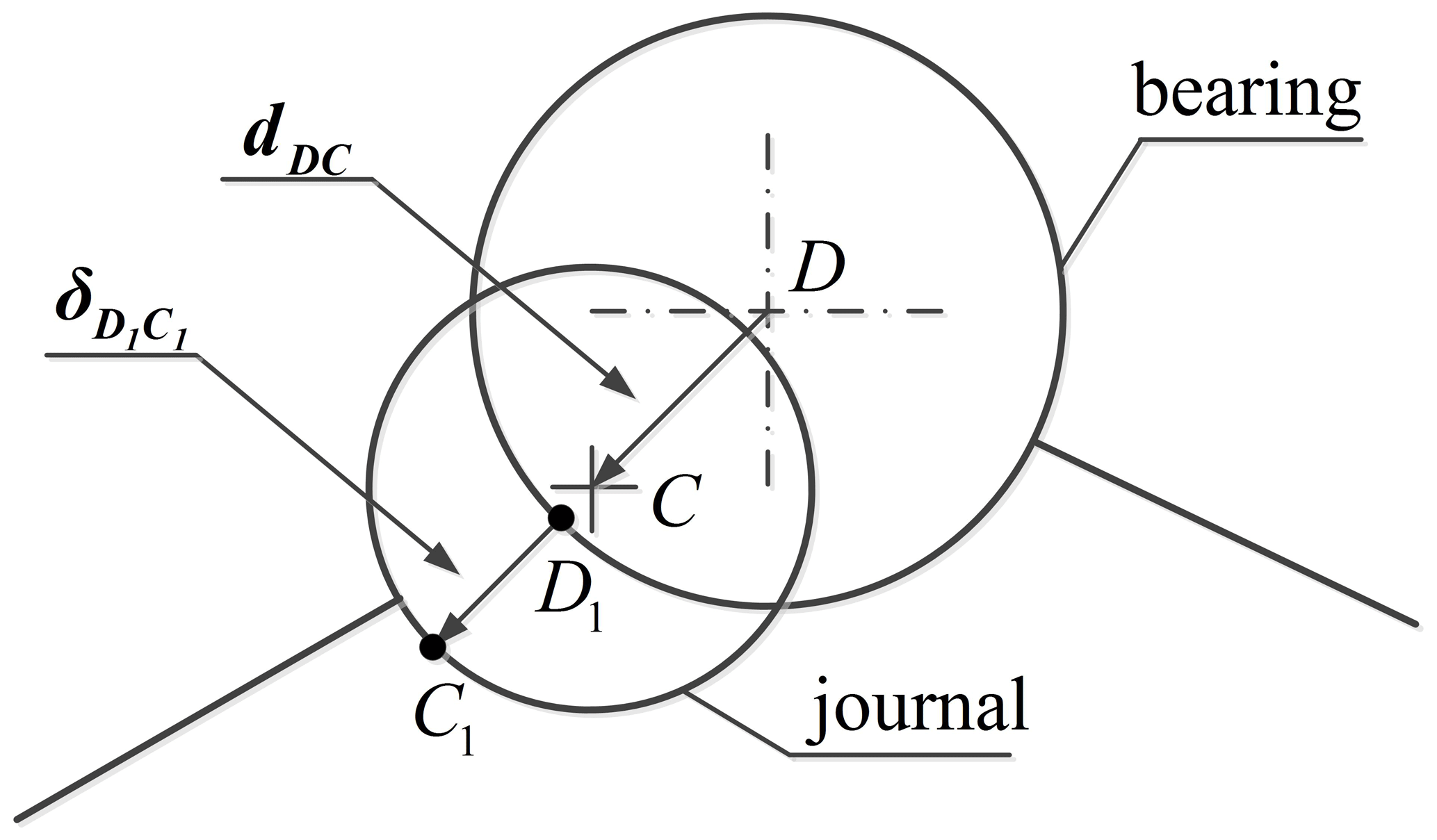
In Fig. 11, C and D are the centers of the journal and the bearing, respectively, and r_C and r_D are coordinate vectors of points C and D. The eccentricity vector d_DC which connects the centers of the bearing and the journal is expressed as

$$\begin{array}{}\text{(11)}& {\mathit{d}}_{\mathrm{DC}}={\mathit{r}}_{\mathrm{C}}-{\mathit{r}}_{\mathrm{D}},\end{array}$$

Then the penetration depth in the clearance joint can be expressed as

$$\begin{array}{}\text{(12)}& {\mathit{\delta }}_{\mathrm{DC}}=\left|{\mathit{d}}_{\mathrm{DC}}\right|-(R_{\mathrm{2}}-R_{\mathrm{1}}),\end{array}$$

where R₁ and R₂ are the radii of the journal and the bearing, respectively.

Figure 12 Flow chart of simulation solution.

Figure 13 Center trajectories of the journal and bearing.

The unit normal vector at the contact point is expressed as

$$\begin{array}{}\text{(13)}& {\mathit{n}}_{\mathrm{DC}}={\displaystyle \frac{{\mathit{d}}_{\mathrm{DC}}}{\left|{\mathit{d}}_{\mathrm{DC}}\right|}},\end{array}$$

Then the coordinate vectors of contact points C₁ and D₁ are calculated by

$$\begin{array}{}\text{(14)}& \left\{\begin{array}{l}{\mathit{r}}_{{\mathrm{C}}_{\mathrm{1}}}={\mathit{r}}_{\mathrm{C}}+R_{\mathrm{1}}{\mathit{n}}_{\mathrm{DC}}\\ {\mathit{r}}_{{\mathrm{D}}_{\mathrm{1}}}={\mathit{r}}_{\mathrm{D}}+R_{\mathrm{2}}{\mathit{n}}_{\mathrm{DC}}\end{array},\right.\end{array}$$

The relative penetration velocity between the journal and bearing can be expressed as

$$\begin{array}{}\text{(15)}& {\mathit{v}}_{{\mathrm{D}}_{\mathrm{1}}{\mathrm{C}}_{\mathrm{1}}}={\dot{\mathit{r}}}_{{\mathrm{C}}_{\mathrm{1}}}-{\dot{\mathit{r}}}_{{\mathrm{D}}_{\mathrm{1}}}.\end{array}$$

The normal contact velocity and the tangential contact velocity between the journal and the bearing are expressed as

$$\begin{array}{}\text{(16)}& \left\{\begin{array}{l}{\mathit{v}}_{\mathrm{n}}=\left({\mathit{v}}_{{\mathrm{D}}_{\mathrm{1}}{\mathrm{C}}_{\mathrm{1}}}\cdot {\mathit{n}}_{\mathrm{DC}}\right){\mathit{n}}_{\mathrm{DC}}\\ {\mathit{v}}_{\mathrm{t}}={\mathit{v}}_{{\mathrm{D}}_{\mathrm{1}}{\mathrm{C}}_{\mathrm{1}}}-{\mathit{v}}_{\mathrm{n}}\end{array}.\right.\end{array}$$

Contact force F_N and friction force F_T now can be obtained by using Eqs. (6) and (9).

The change of temperature results in the change of component stiffness, and correspondingly; the stress-free length of the component changes. When the component length is varied with time or temperature, the center positions of the journal and the bearing change, resulting in the variation of the contact force and friction force.

4.2 Computational strategy of dynamic equations

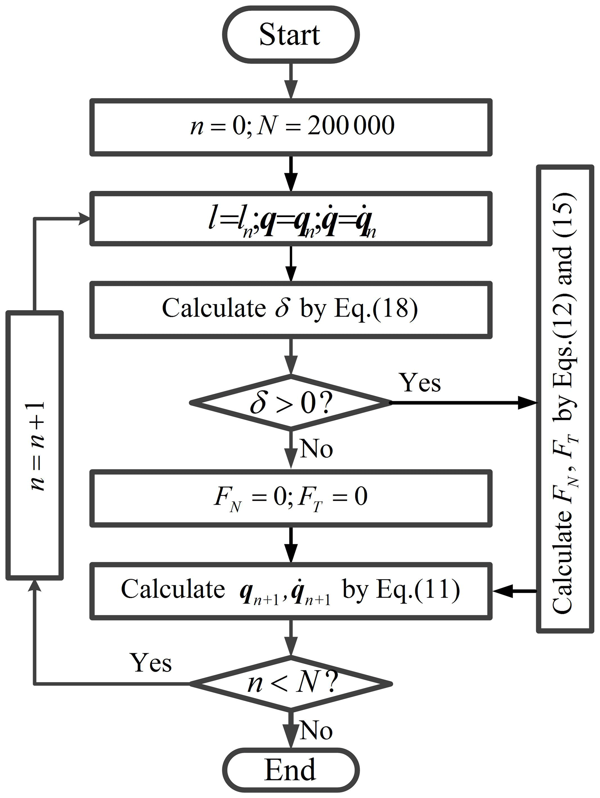
The fourth-order Runge–Kutta method is used to solve dynamic equations, and the flow chart of the solving process is shown in Fig. 12.

1. Give the total number of iterations as N and set the current iteration number as n=0.

2. Update the generalized displacement as q_n, the generalized velocity ${\dot{\mathit{q}}}_n$ and the component length l_n.

3. Calculate the penetration depth δ using Eq. (12).

4. If the journal and bearing are in contact (δ>0), calculate F_N and F_T using Eqs. (6) and (9), otherwise, set $F_{\mathrm{N}}=F_{\mathrm{T}}=\mathrm{0}$.

5. Calculate the generalized displacement q_n+1 and generalized velocity ${\dot{\mathit{q}}}_{n+\mathrm{1}}$ using Eq. (5).

6. If n<N, set $n=n+\mathrm{1}$ and return to step (2), otherwise, end the simulation.

4.3 State jump and control in deployable structure

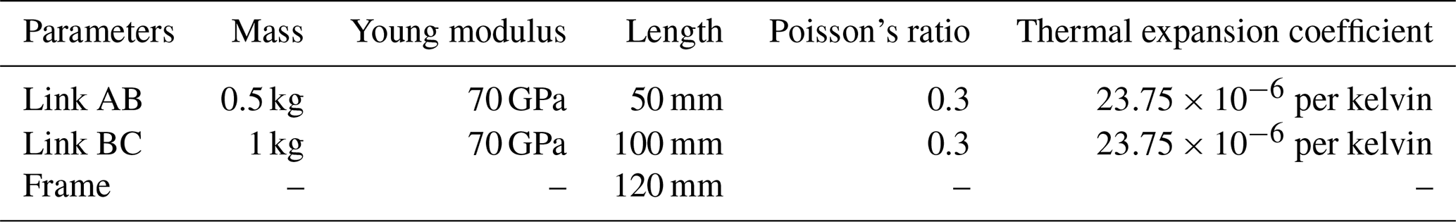
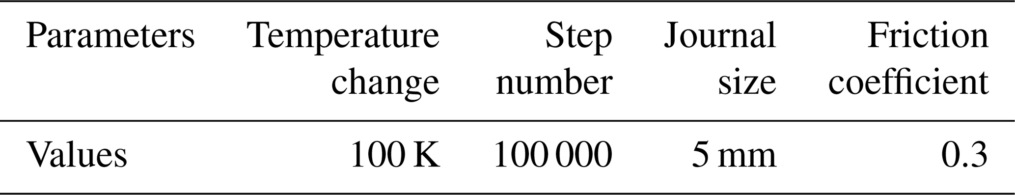
For the above-mentioned clearance structure, geometric and material parameters are shown in Table 2 and simulation parameters are shown in Table 3. At the initial moment, the center of the journal and the bearing are coincident, and the generalized velocity and acceleration are set as 0. The joints between the links and the frame are assumed to be ideal and the clearance size of the joint between AB and BC is 0.1 mm. The temperature increases linearly from 0 to 100 K in the first half of loading and then decreases linearly to 0 K.

Table 2 Geometric and material parameters of deployable structure.

Table 3 Simulation parameters of dynamic solution process.

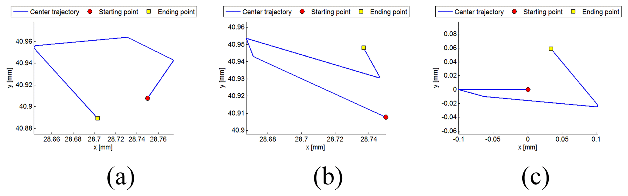
Simulation results are shown in Fig. 13. Curves in Fig. 13a and b are the center trajectories of the journal and the bearing, respectively, and Fig. 13c shows the trajectory of the bearing center relative to the journal center. As can be seen from Fig. 13, relative positions of deployable structural members will change while the temperatures before and after loading are the same; that is, the state jump phenomenon occurs.

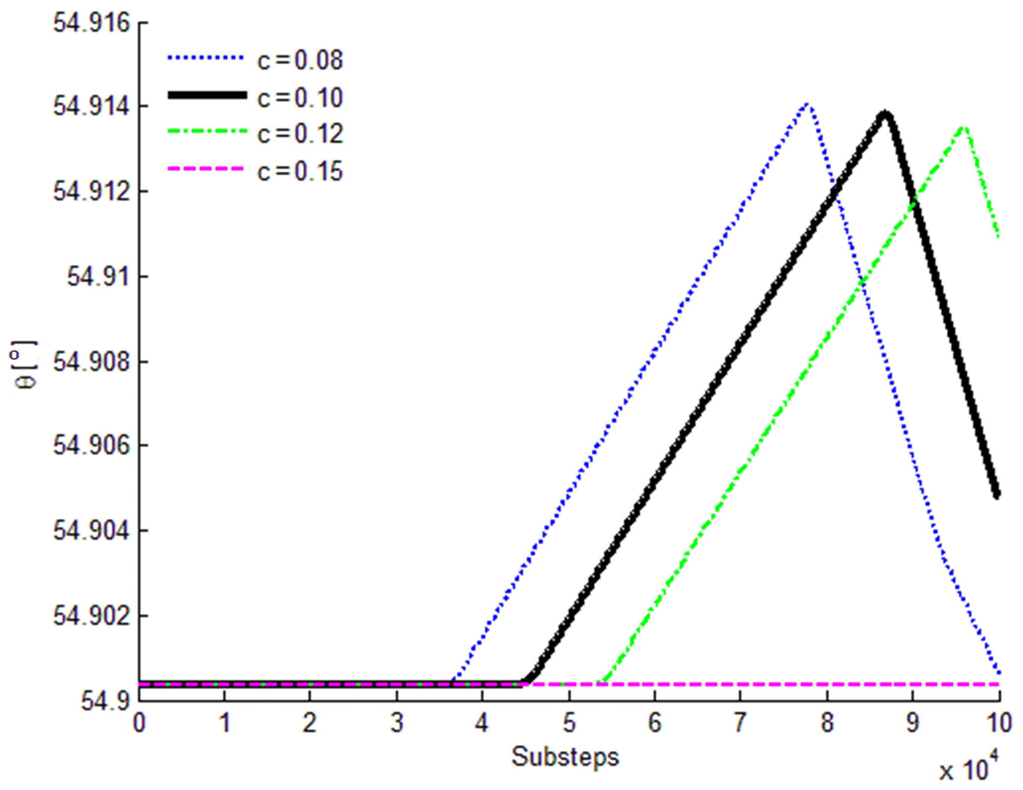
Deflection angle curves of AB under different clearance sizes are shown in Fig. 14. It is shown that the deflection angle of AB varies with the clearance size. The smaller the clearance is, the earlier the deflection occurs. When the clearance size is large enough (greater than the maximal thermal deformation), AB and BC do not come into contact during the whole loading process.

Figure 14 Deflection angle of AB under different clearance sizes.

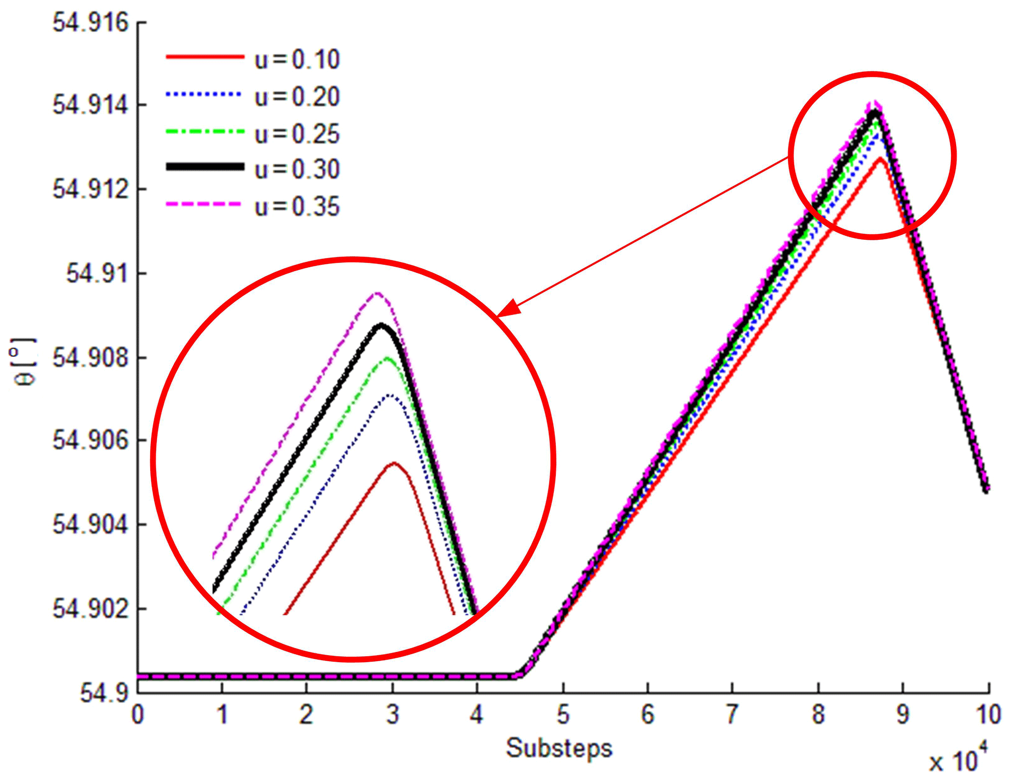
Deflection angle curves of link AB under different friction coefficients are shown in Fig. 15. It is shown that the deflection angle of AB varies with the friction coefficients. Generally speaking, the larger the friction coefficient, the larger the range of the deflection angle.

Figure 15 Deflection angle of AB under different friction coefficients.

One torsion spring is added to the clearance joint of the deployable structure, and its effect on the state jump phenomenon is analyzed. The torque M provided by the torsion spring with an angle α is

$$\begin{array}{}\text{(17)}& M=K_M{\mathrm{\Delta }}_{\mathit{\sigma }}=K_M(\mathit{\alpha }-{\mathit{\alpha }}_{\mathrm{0}}),\end{array}$$

where α is the flare angle, α₀ is the flare angle of torsion spring in the free state and K_M is the elastic coefficient of torsional spring. The effect of torsional spring on the structure is equivalent to the external force varying with the flare angle.

The torsion spring is assumed to be in the stress-free state when the structure is in ideal position (the center of the journal coincides with that of the bearing), and the deflection angle of AB under different elastic coefficients is shown in Fig. 16.

Figure 16 Deflection angle of AB under different elastic coefficients.

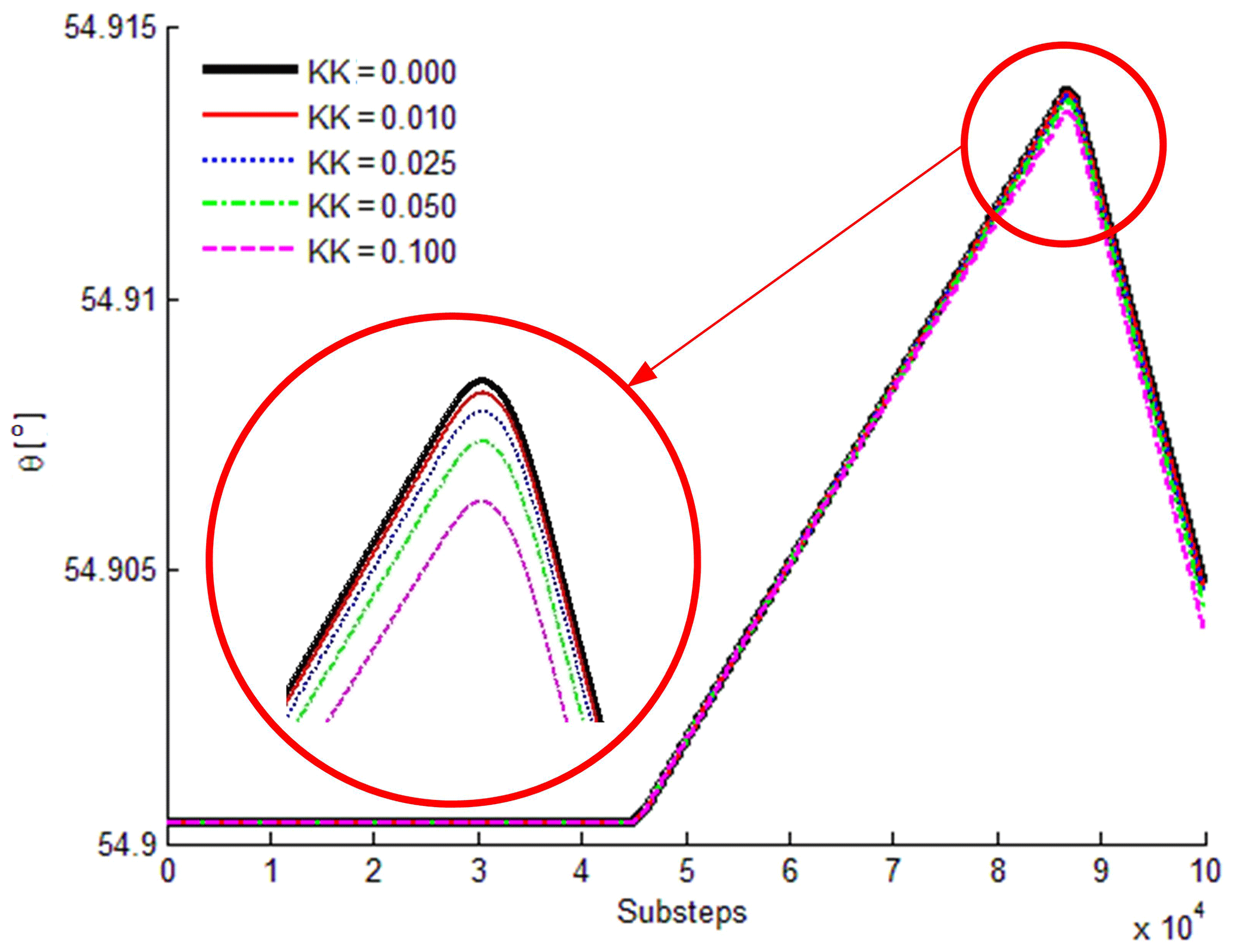
It can be seen from Fig. 16 that the state jump value will change when the torsion spring is installed in the clearance joint. The deflection angle decreases with the increase in the elastic coefficient of the torsion spring, in a certain range. Therefore, by using reasonable methods, the state jump phenomenon in deployable structures can be controlled.

5 Conclusion

In this paper, the static multiple-stable-state phenomenon in clearance joints of deployable structures is clarified through force analysis. An equivalent model consisting of a variable stiffness spring and a contact element is proposed, which can capture the state jump phenomenon in deployable structures. The control methods have been presented for reducing the effect of state jump on structural responses. Numerical results of the deployable structure of an umbrella-shaped antenna have verified the proposed analysis method. Some conclusions have been summarized in the following.

• a.

  Clearance and friction in kinematic joints are the basic reasons for the generation of the state jump phenomenon.

• b.

  The magnitude of friction and axial stiffness of components are the main factors affecting the state jump value.

• c.

  The state jump phenomenon can be controlled by reasonable measures, such as reducing the friction force, increasing the stiffness of structure components and adding pre-stressed springs to the structure.

6 Future work

Future work will focus on improving the performance of the space deployable structure under complex temperature loads.