the Creative Commons Attribution 4.0 License.
the Creative Commons Attribution 4.0 License.
 | 30 Oct 2019
Effects of friction models on simulation of pneumatic cylinder
Van Lai Nguyen
Khanh Duong Tran
This study examines effects of three friction models: a steady-state friction model (SS model), the LuGre model (LG model), and the revised LuGre model (RLG model) on the motion simulation accuracy of a pneumatic cylinder. An experimental set-up of an electro-pneumatic servo system is built, and characteristics of the piston position, the pressures in the two-cylinder chambers and the friction force are measured and calculated under different control inputs to the proportional flow control valves. Mathematical model of the electro-pneumatic servo system is derived, and simulations are carried out under the same conditions as the experiments. Comparisons between measured characteristics and simulated ones show that the RLG model can give the best agreement among the three friction models while the LG model can only simulate partly the stick-slip motion of the piston at low velocities. The comparison results also show that the SS model used in this study is unable to simulate the stick-slip motion as well as creates much oscillations in the friction force characteristics at low velocities.
- Article
(7094 KB) - Full-text XML
-
Supplement
(35251 KB) - BibTeX
- EndNote


Friction usually exists between piston/rod seals and contacting surfaces in fluid power cylinders and has an important aspect in fluid power control systems. Friction may occur in nonlinear manner and cause limit cycles and unexpected stick-slip oscillation at low operating velocities. These nonlinear characteristics of the friction make accurate simulation and position control of the fluid power cylinders difficult to achieve. In order to overcome these difficulties, it is, therefore, necessary to develop an accurate friction model for the fluid power cylinders.
Classical friction models that describe the steady-state relation between velocity and friction force, which can be characterized by the viscous and Coulomb friction with Stribeck effect combination have been proposed (Hibi and Ichikawa, 1977; Armstrong, 1991; Armstrong et al., 1994; Pennestrì et al., 2016; Marques et al., 2016, 2019; Brown and McPhee, 2016). However, some friction behaviours cannot be captured by these classical friction models, as for example, hysteretic behaviour with oscillating velocity, stiction behaviour and breakaway-force variations (Armstrong et al., 1994). In addition, in the mechanics-related controller design, simple classical models are not enough to address applications with high precision positioning requirements and low velocity tracking. Thus, in order to obtain accurate friction compensation and best control performance, a friction model with dynamic behaviours is necessary.
Several friction models that describe the dynamic behaviours of friction have been proposed so far (Haessig and Friedland, 1991; Canudas et al., 1995; Dupont, 1995; Swevers et al., 2000; Dupont et al., 2002), and among them, the LG model (Canudas et al., 1995) is most widely utilized in control applications (Lu et al., 2009; Freidovich et al., 2010; Hoshino et al., 2012; Green et al., 2013; Ahmed et al., 2015; Wojtyra, 2017; Piatkowski and Wolski, 2018). The model can simulate arbitrary steady-state friction characteristics and it can capture hysteretic behaviour due to frictional lag, spring-like behaviour in stiction and give a varying break-away force depending on the rate of change of the applied force. However, Yanada and Sekikawa (2008) have shown that the LG model cannot simulate a decrease of the maximum friction force observed after one cycle of the velocity variation in a hydraulic cylinder when the piston velocity varies sinusoidally with velocity reversals. In order to overcome this limitation of the LG model, they have modified the LG model by incorporating lubricant film dynamics into the model to obtain a new friction model called the modified LuGre model (MLG model).
Next, Tran et al. (2012) have pointed out that the MLG model cannot simulate the real hysteretic behaviours of the friction force–velocity curve in the fluid lubrication regime of hydraulic cylinders. The MLG model was then improved by replacing the usual fluid friction term, which is proportional to velocity, with a first-order lead dynamic. It has been verified that the improved model, called the new modified LuGre model (NMLG model), can capture accurately most of the friction behaviours observed in the hydraulic cylinders (Tran et al., 2012) and in the pneumatic cylinders (Tran and Yanada, 2013) in entire sliding regime. In addition, the usefulness of the NMLG model in simulating the operating characteristics of a hydraulic servo system have been verified by Tran et al. (2014). In a recent study, Tran et al. (2016) have shown that the NMLG model cannot capture the friction characteristics observed experimentally in pneumatic cylinders when the pneumatic cylinders operated in pre-sliding regime and they have proposed a new friction model by incorporating a hysteresis function into the NMLG model. Although the usefulness of the new friction model, called the revised LuGre model (RLG model) in this study has been verified, the validity of this model in simulating the motion of electro-pneumatic servo systems has not been investigated.
In this paper, the effects of the RLG model on the simulation accuracy of an electro-pneumatic servo system are examined in comparation with the LG model and a SS model (static + Coulomb + viscous friction). For this purpose, an experimental setup of the electro-pneumatic servo system using a pneumatic cylinder is proposed. Characteristics of the piston position, the pressures in the cylinder chambers and the friction force of the piston are measured and analysed under various operating conditions of control inputs to proportional flow control valves. Mathematical model of the electro-pneumatic system is developed by incorporating one of the three friction models into the entire system model, and the pneumatic cylinder's characteristics are simulated using MATLAB/Simulink under the same conditions as the experiments. Comparisons of simulation and experimental results are carried out to show the effects of each friction model and to verify the validity of the RLG model for pneumatic cylinders.
The organization of this paper is as follows: Brief descriptions of the SS model, the LG model, and the RLG model are given in Sect. 2. Section 3 describes the electro-pneumatic servo system and its mathematical model. Experimental and simulation results are presented and discussed in Sect. 4. Finally, main conclusions are drawn in Sect. 5.
In this section, the three friction models: the SS model, the LG model and the RLG model are described in short.
2.1 Steady-state friction model
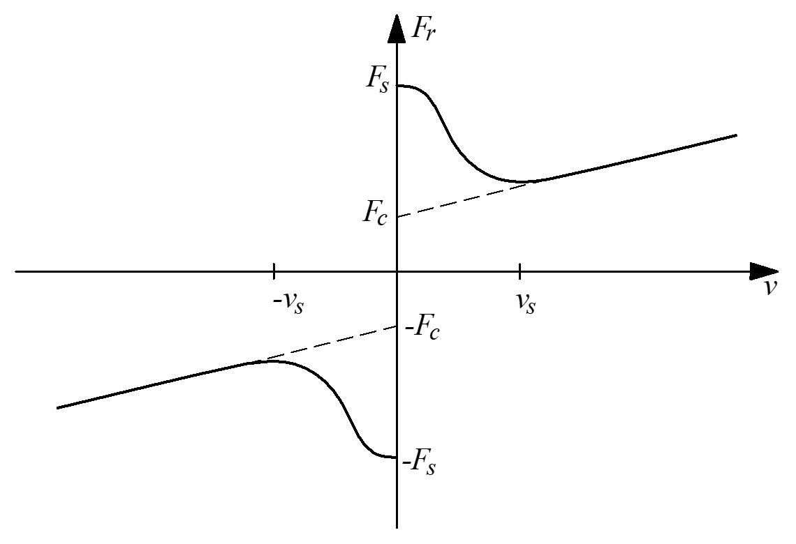
The SS model used in this study is a combination of static friction, Coloumb friction and viscous friction (Armstrong, 1991). The model characteristics are presented by a Stribeck curve as shown in Fig. 1. In this friction model, the friction force Fr depends on the velocity input and is calculated by the following equation:
where Fs is the static friction force, Fc is the Coulomb friction force, vs is the Stribeck velocity, n is the exponent that affects the slope of the Stribeck curve, σ2 is the viscous friction coefficient and v is the relatively tangential velocity between two contacting surfaces.
2.2 LuGre model
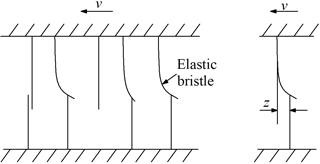
The LG model (Canudas et al., 1995) is a combination of a stiction force with an arbitrary steady-state friction force which can include the Stribeck effect. It is assumed in this model that two matting surfaces make contact at several asperities through elastic bristles as shown in Fig. 2. When a tangential force is applied to a surface, the bristles will deflect like springs; and when the force is sufficiently large, some of the bristles will break and then slip. The mean deflection of the elastic bristle is denoted as z and is defined as:
where σ0 is the stiffness of the elastic bristle and g(v) is the Stribeck function and is defined as:
The friction force is given by
where σ1 is the micro-viscous friction coefficient.
In Eq. (4), the first two terms represent the friction force generated from the bending of the elastic bristles and the third term stands for the viscous friction. In steady-state condition, the friction force is given by Eq. (1).
2.3 Revised LuGre model
The RLG model (Tran et al., 2016) is a model where three modifications were made from the LG model. Firstly, a lubricant film dynamic has been incorporated into the function g(v) in Eqs. (2) and (3) to obtain a new Stribeck function g(v,h) as shown in Eqs. (5) and (6). Secondly, the friction force term σ0z in Eqs. (2) and (4) of the LG model has been replaced by a hysteresis function F(z) as shown in Eqs. (5) and (7). And thirdly, the usual fluid friction term σ2v in Eq. (4) has been replaced by a first order lead dynamics as shown in Eq. (7).
where T is the time constant for fluid friction dynamics. h is the dimensionless lubricant film thickness and is given by
where hss is the dimensionless steady-state lubricant film thickness parameter, Kf is the proportional constant for lubricant film thickness, vb is the velocity within which the lubricant film thickness is varied, and τhp,τhn and τh0 are the time constants for acceleration, deceleration, and dwelling periods, respectively. In Eq. (9), h≤hss corresponds to the acceleration periods and h>hss corresponds to the deceleration periods. It is noted that the lubricant used for the packing of pneumatic cylinders is grease and is not oil. Regarding the behaviour of film formation of grease between contact surfaces, it has been shown by Li et al. (2009) that the film thickness becomes thinner during acceleration and thicker during deceleration than the steady-state film thickness. This behaviour of grease film is the same as that of oil film in Sugimura et al. (1998). Therefore, it is believed that the lubricant film dynamics described by Eqs. (8) to (11) hold also for grease and can be applied to pneumatic cylinders.
The hysteresis function F(z) in Eq. (5) is a function that simulates the hysteresis behaviour with nonlocal memory in pre-sliding regime. F(z) consists of many functions fi(z) (i=1, 2…) in which each function fi(z) models a segments of transition curve. The friction force-deflection curve in pre-sliding regime of the pneumatic cylinder consists of transition curves, i.e. curves between velocity reversal points (Tran et al., 2016). Each velocity reversal starts a new transition curve and each transition curve can be divided into some segments depending on its shape. Each segment can be approximated by a function fi(z) as follows:
where ci and ki are the segment parameters that can be identified from experimental friction force-displacement characteristics, ciki indicates the stiffness of the bristles at z=zi, zi is the initial deflection on the ith segment, and fi(zi) is the initial friction force of the ith segment and equals to the final friction force of the (i−1)th segment.
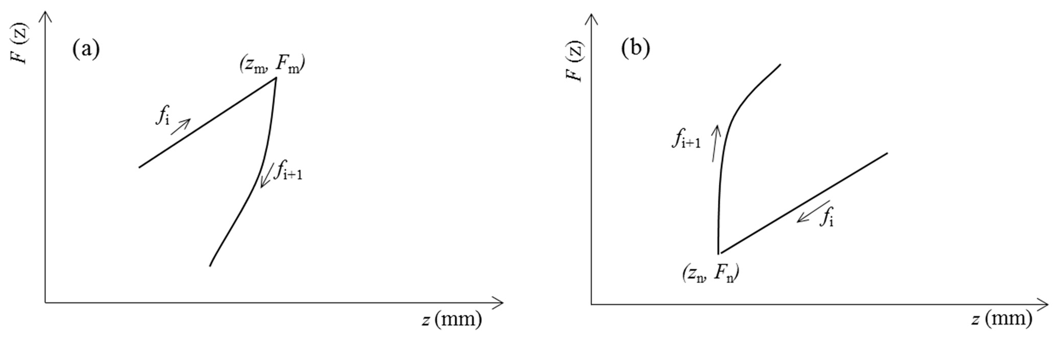
Implementation of the function F(z) in pre-sliding regime requires two memory sets for the functions fi(z): one for ascending curves (v>0) and one for descending curves (v<0). The sets begin at velocity reversal and remove when a hysteresis loop is closed. At each inverse point of velocity, the deflection z takes a maximum value zm (Fig. 3a) or a minimum value zn (Fig. 3b). At these points, a new transition curve begins and the function fi+1(z) is calculated by resetting zi in Eq. (12) to zm or zn and fi(zi) will take the value Fm or Fn, respectively.
For internal loops created on an ascending curve (Fig. 4a) and on a descending curve of external loop (Fig. 4b), the internal loop is formed by two curves 2 and 3 between two velocity reversal points at zn and zm. When the velocity reverses at zn, the numerical program will judge the state to be on the internal loop by checking the variation of velocity sign from positive to negative. The state is calculated by a function fi+1(z) using the parameters ci+1, ki+1 and the values of zn and Fn. When the velocity reverses at zm, the numerical program will remain the state on the internal loop and the state is calculated by a function fi+2(z) using the parameters ci+2, ki+2 and the values of zm and Fm. After the velocity reversal point zm, a function fi(z) of the curve 1 on the external loop is calculated together with the function fi+2(z) of the curve 3. When the value of fi+2(z) reaches the value of fi(z) at the point in the vicinity of zn and when there is no change in velocity sign, the friction state has to follow the curve 1 or curve 4 on the external loop after the intersection point zn. The values of zn, Fn, zm and Fm of the internal loop are automatically cleared from the program after the intersection point zn.
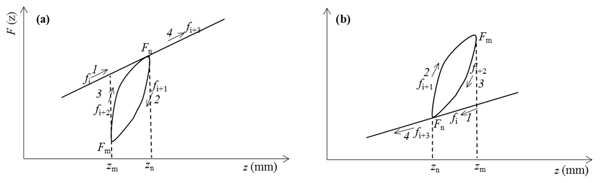
Figure 4Numerical implementation of internal hysteresis loop: (a) internal loop on an ascending external curve, (b) internal loop on a descending external curve
When the piston movement enters its sliding regime, i.e., when the deflection reaches Fs∕σ0, the model is then switched to the NMLG model. At this condition, the hysteresis function F(z) is set equally to σ0z.
In steady-state condition, friction force is described by
The static parameters Fs, Fc, vs, vb, n, and σ2 of the three models are identified from measured steady-state friction characteristics using the least-squares method and the dynamic parameters σ0, σ1, τh, and T are identified from measured dynamic friction characteristics by the methods proposed in Tran et al. (2012). The function fi(z) is identified from measured friction force-displacement characteristics by the methods proposed in Tran et al. (2016).
In this section, an experimental test setup of the electro-pneumatic servo system is firstly introduced, and its mathematical model is then developed.
3.1 Experimental test setup
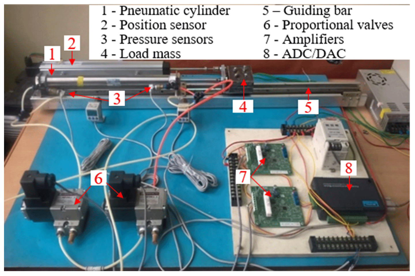
Figures 5 and 6 show the experimental test setup used in this investigation. The system consists of a pneumatic cylinder (Eq. 1) (SMC, CM2L25-300) fixed horizontally on a flat plate made of steel. The cylinder has internal diameter of 0.025 m, rod diameter of 0.01 m and piston stroke of 0.3 m, respectively. The piston end was connected to a load mass (Eq. 4) which can slide on a guiding bar (Eq. 5). The load mass was varied from 0.5 to 5 kg. The piston motion was controlled by two flow proportional control valves (Eq. 6) (SMC, VEF3121). The two valves can supply a flow rate up to 720 L min−1 with a rated voltage of 5 VDC. According to the valve characteristic, if the valve control inputs u1 or u2 vary from 2.5 to 5 VDC, the valves will provide air into the cylinder chamber (the valves are operated at left position); and if the valve control inputs u1 or u2 vary from 0 to 2.5 VDC, the valves will release air into the atmosphere (the valves are operated at right position). Therefore, by combining signals between u1 and u2 of the two valves, the extending and retracting motions of the piston can be obtained.
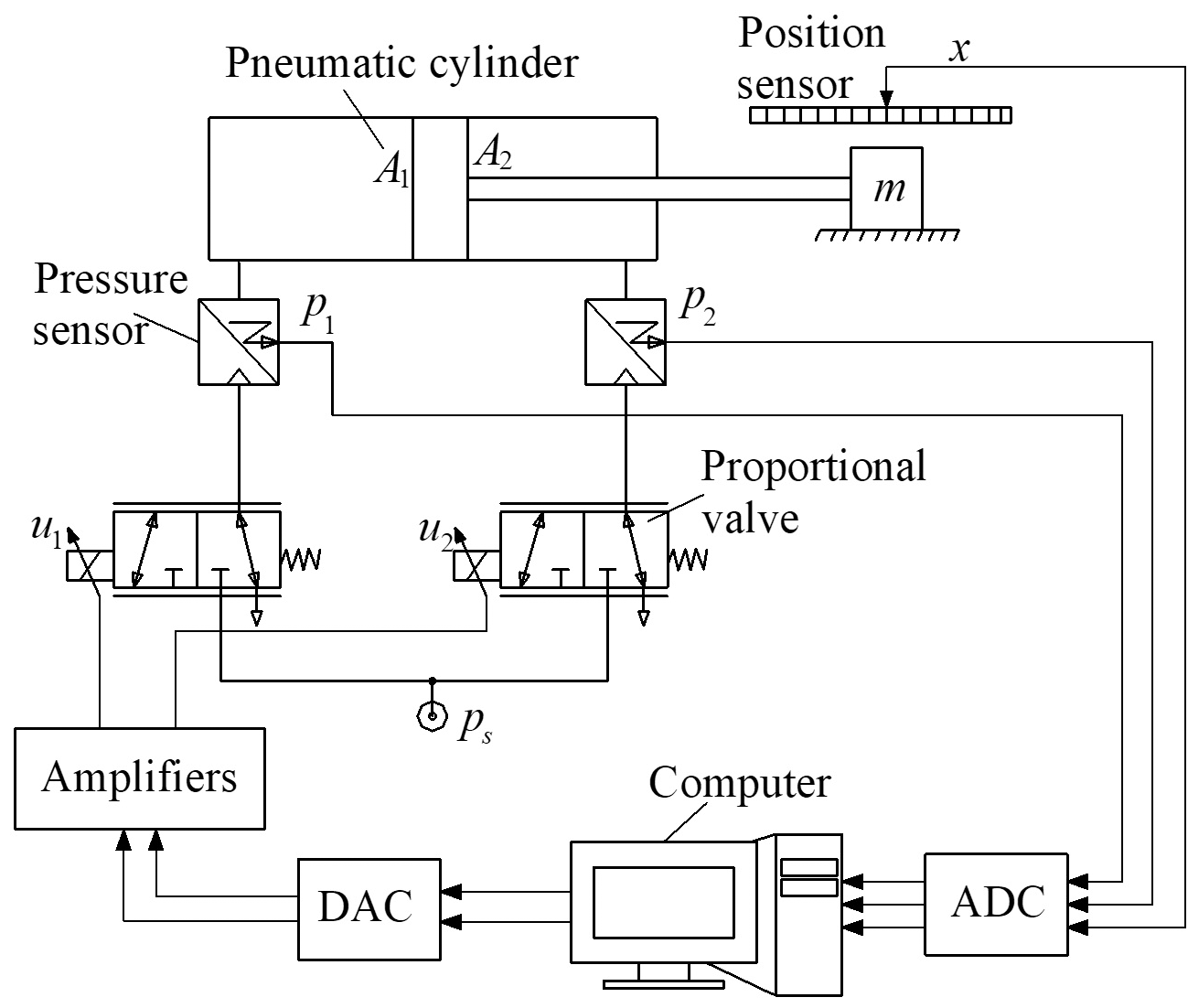
The position of the piston was measured by a position sensor (Eq. 2) with a measurement range of 300 mm (Novotechnik, LWH0300). The pressures in the two-cylinder chambers were measured by two pressure sensors (Eq. 3) with a measurement range of 1 MPa (SMC, PSE540). Measuring accuracies of the position sensor and the pressure sensors are less than 0.5 % F.S and 1 % F.S, respectively. The source pressure was set at 0.5 MPa. The position signal and the pressure signals were read via a personal computer through a 12 bits analog to digital converter (ADC). The computer sent the control signals u1 and u2 to the two valves through a 12 bits digital to analog converter (DAC) (Eq. 8) (Advantech, USB4711). Two amplifiers (Eq. 7) (SMC, VEA250) were used to convert the voltage signals to the current signals of the valves. The program for data acquisition was done by using Microsoft visual C software. The signals were recorded at the interval of 1.16 ms.
The friction force, Fr, was obtained from the equation of motion of the pneumatic piston using the measured values of the pressures in the cylinder chambers, the acceleration of the piston and the weight of the load mass as follows:
where A1 and A2 are the piston areas, M is the total mass of the piston, piston rod and the external load. a is the piston acceleration and was calculated by an approximation of second differentiation of the measured piston position. The noise in the calculated acceleration signal was filtered by an acausal first order low-pass filter with a bandwidth of 32 Hz.
3.2 Modelling of the electro-pneumatic servo system
The objective of this section is to derive the dynamic equations of the entire electro-pneumatic servo system. In order to obtain the air flow dynamics in the pneumatic cylinder, the following assumptions are used:
- a.
The used air is an ideal gas and its kinetic energy is negligible in the cylinder chamber.
- b.
The leakages of the cylinder are negligible.
- c.
The temperature variation in cylinder chambers is negligible with respect to the supply temperature.
- d.
The pressure and the temperature in the cylinder chamber are homogeneous.
- e.
The evolution of the gas in each chamber is polytropic process.
- f.
The supply and ambient pressures are constant.
As mentioned in Sect. 3.1, if the supplied voltage to the proportional valve varies from 2.5 to 5 VDC, the valve will provide air into the cylinder chamber (the building pressure case) and if the supplied voltage varies from 0 to 2.5 VDC, the valve will release air into the atmosphere (the exhausting pressure case). In addition, it is noted that the proportional valves are overlap and there exists a dead zone in relation between the mass flow rate and the voltage signal of the valves. Therefore, the mass flow rates (j=1 and 2) that flow into or out from the chambers of the pneumatic cylinder can be derived in terms of the voltage inputs uj of the two valves as follows:
where um and un are respectively the upper and lower voltage limits of the dead-zone, ps and pj respectively the source air pressure and the pressure in the chamber j of the cylinder, R is the gas constant, k is the specific heat ratio, Ts is the temperature of the supply source, and KV1 and KV2 are respectively the valve gains for the building pressure case and the exhausting pressure case. The operating condition corresponds to the case when the pressure in the chamber j is the building pressure, to the case when the pressure in the chamber j is the exhausting pressure, and to the case when all the valve ports are closed (the dead-zone condition of the valve). γjb and γje are respectively the modifying factors when the pressure in the chamber j is building pressure and exhausting pressure. These factors are given by Tressler et al. (2002) as follows:
where patm is the atmosphere pressure.
The dynamic relationships between the mass flow rates , and the pressures p1, p2 in the cylinder chambers can be obtained with basis on energy conversation arguments in a pneumatic cylinder and are given by Hodgson et al. (2012) as follows:
where v is the piston velocity. V1 and V2 refer to the volumes of the cylinder chambers 1 and 2, respectively and are calculated as:
where L is the piston stroke, x is the piston position, and V10 and V20 are the dead volumes in the cylinder chambers 1 and 2 respectively.
Motion equation of the cylinder piston according to Newton's second law is given by
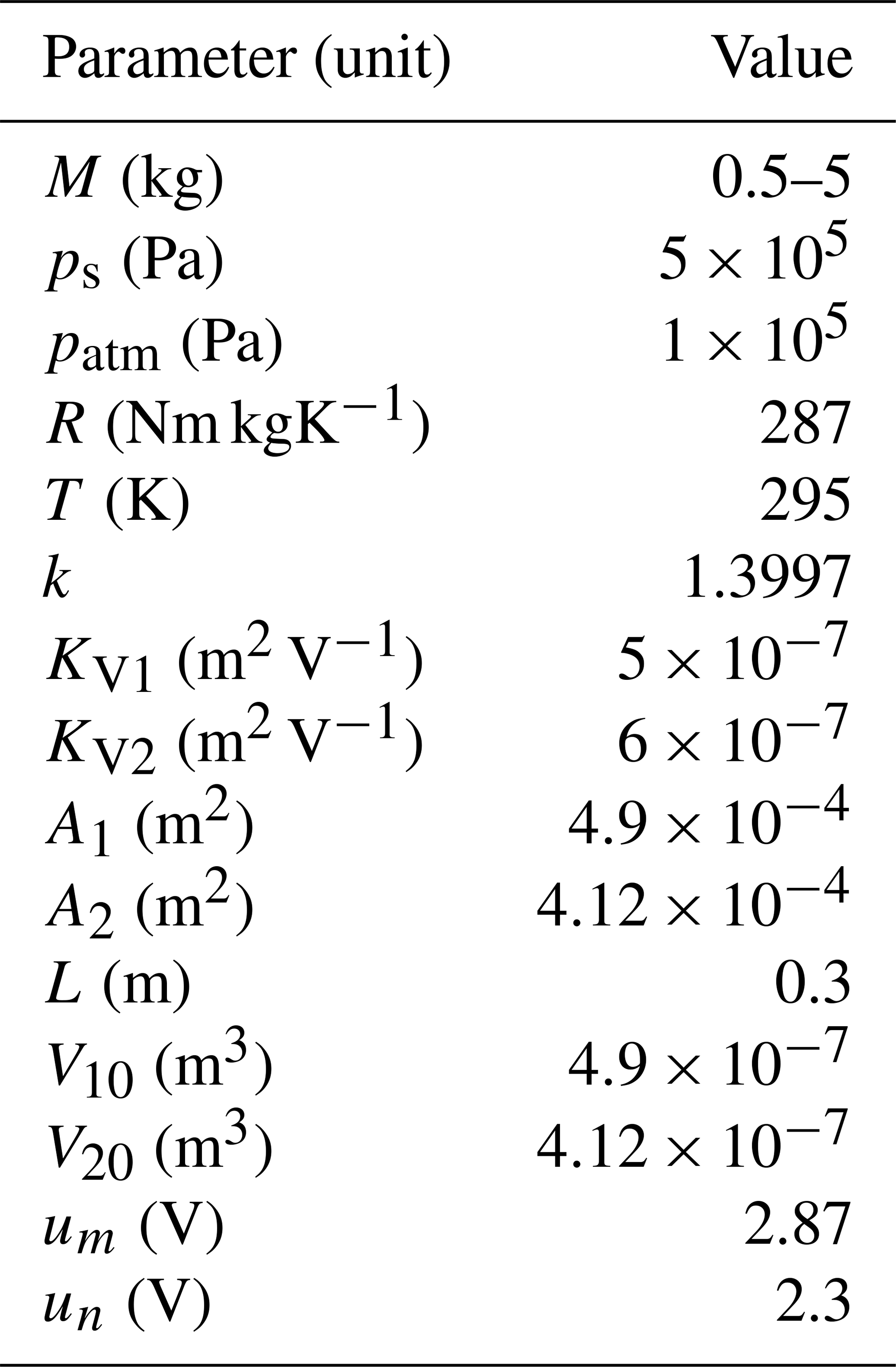
where Fr is the friction force which has been described by one of the three friction models in Sect. 2. The system parameters used in simulation are shown in Table 1. The parameters of um and un were determined from the measured characteristics of the pressures p1 and p2 at constant voltage inputs of the valves. um and un were taken at the voltage values at which the pressure p1 or p2 starts to increase, i.e. the air starts to flow into the cylinder chamber.
In this section, experimental characteristics of the piston position, the pressures in the cylinder chambers, the inertial force and the friction force of the piston under different operating conditions of the voltage signals u1 and u2 are firstly presented and analysed. Comparisons between the simulation results of the three friction models and the experimental results are then presented and discussed to show effects of each friction model.
4.1 Experimental results
Figure 7 shows the measured characteristics of the piston position, the pressures p1 an p2 in the cylinder chambers, the inertial force and the friction force when the valves were supplied by constant voltage values. The control inputs u1 and u2 were given by 2.875 and 2.19 VDC, respectively. For this case, the air from air tank was supplied to the cylinder chamber 1 through the valve 1 and the air in the cylinder chamber 2 was exhausted to the atmosphere through the valve 2. Flow rates of the air supplied to and exhausted from the cylinder chambers in this case are relatively small. As can be seen in Fig. 7a for the position characteristic, the piston firstly remains at an initial position of 0.035 m for 1.8 s then moves a small distance to a new position of 0.045 m. After that the piston suddenly stops and remains at the new position for 0.5 s then the piston moves again. This movement process of the piston is continued until the stroke end of the piston. This characteristic is called “stick-slip” motion and has been observed in pneumatic cylinders (Sakiichi et al., 1988; Peng et al., 2012) and in other mechanisms (Mate et al., 1987; Lampaert et al., 2004; Landolsi et al., 2009). This motion of the piston can be explained that when air is supplied to the chamber 1, air is compressed and the pressure p1 is increased (in Fig. 7b) while the pressure p2 in the chamber 2 is remained at 0 MPa. In the first 1.8 s, the increase in pressure p1 is not large enough to overcome the friction force so that the piston remains stationary. As the pressure p1 rises to a value large enough of about 0.022 MPa, creating an enough force to overcome the friction force, then the piston starts moving (slip). However, as the piston moves, the volume of the chamber 1 expands and the pressure p1 decreases and thus the piston stops moving (stick). Air continues to be fed into the chamber 1 and, after a period, the pressure p1 is increased again to an enough value to overcome the friction force then the piston moves again. The process is then repeated. It is further noted in Fig. 7b that the maximum pressure p1 obtained from the second moving onwards are less than the maximum pressure p1 in the first ones. In Fig. 7c, the inertial force obtained is small and therefore variation of the friction force (Fig. 7d) is similar to that of the pressure p1. Value of the friction force is maximum (10.5 N) at the time when the piston starts moving. When the piston has moved, the friction force decreases. In the next cycles, the value of the friction force varies between 4.5 to 8.4 N.

Figure 7Experimental characteristics at operating conditions of u1=2.875 V, u2=2.19 V and M=1.3 kg: (a) piston position, (b) pressures in the cylinder chambers, (c) initial force, (d) friction force.
When the signal u1 of the valve 1 was given by a higher value (u1=2.99 V) and u2 of the valve 2 was given by a lower value (u2=2.09 V) than those in case of Fig. 7, the piston remains at the initial position 0.03 m for 0.45 s then moves smoothly to a new position of 0.24 m at 1.4 s as shown in Fig. 8a. Stick-slip motion of the piston cannot be observed. It is noted that the air flow rate supplied to the cylinder chamber 1 is relatively large in this case. This means that if the air is provided largely enough to the cylinder chamber in a short time, a continuous motion of the cylinder piston can be obtained. In addition, it is shown in Fig. 8b that due to a large amount of the air flow rate supplied to the cylinder chamber 1, the pressure of p1 continues increasing after the piston has moved. The pressure is increased to the maximum value of about 0.03 MPa at 0.58 s and then slightly decreased. Although the maximum inertial force in Fig. 8c is larger than that in Fig. 7d, the variation of the friction force in Fig. 8d is also mainly depend on the variation of the pressure p1.

Figure 8Experimental characteristics at operating conditions of u1=2.99 V, u2=2.09 V and M=1.3 kg: (a) piston position, (b) pressures in the cylinder chambers, (c) initial force, (d) friction force.
Such similar above behaviours can be also observed for the cases when the piston retracts, i.e. for case when the valve 2 supplies air to the cylinder chamber 2 and the valve 1 exhausts air from the cylinder chamber 1 to the atmosphere.
Figure 9 shows the experimental characteristics of the pneumatic cylinder when the valve signals u1 and u2 were varied with sinusoidal waves. The signals of the valves were given by and with a low frequency of 0.2 Hz. It can be seen in Fig. 9a that the piston moves in a trapezoidal form with the corresponding frequency of the valve signals and the position amplitude tends to increase slightly after each cycle. Like the results in Figs. 7 and 8, the piston moves only when the pressure p1 in the extending stroke or p2 in the retracting stroke is increased to a value large enough, corresponding to the appropriately increased and decreased values of the valve signals u1 and u2. In the extending stroke of the piston, the increase of pressure p1 is relatively large, to a maximum value of 0.04 MPa, while the increase of the pressure p2 is very small, near the atmosphere pressure. In contrast, the increase of pressure p2 is relatively large, to a maximum value of 0.0506 MPa, while the increase of the pressure p1 is very small in the retracting stroke (Fig. 9b). The peaks of the pressure p2 in the retracting stroke are higher than those of the pressure p1 in the extending stroke. This result is due to a difference in the piston areas. The friction force observed in Fig. 9d varied in a sinusoidal form and the variation of the friction force is repeated in each cycle. It can be realized that this variation of the friction force in the pneumatic cylinder is different from that observed in hydraulic cylinders (Tran et al., 2012). In hydraulic cylinders, the friction force characteristic hydraulic cylinders showed a decrease of the maximum friction force observed after one cycle of the velocity variation.

Figure 9Experimental characteristics at operating conditions of (V), (V), f=0.2 Hz, M=1.3 kg: (a) piston position, (b) pressures in the cylinder chambers, (c) initial force, (d) friction force.
4.2 Simulation results
This section shows comparisons between the simulated results of the three friction models (the RLG model, the LG model, and the SS model) and the measured results. Simulations were done using MATLAB/Simulink. An ode3 solver with a fixed-time step of s was chosen for numerical integration algorithm. The parameter values of the three friction models used in these simulations are shown in Table 2. These values were taken from Table 2 in Tran et al. (2016) in which the static parameters of the models, Fs, Fc, vs, vb, n, and σ2, were identified experimentally from the steady-state friction characteristics using the least-squares method and the dynamic parameters, σ0, σ1, τh, and T were identified experimentally by the method proposed by Tran et al. (2012).
Table 2Values of the parameters of the three models used in simulation.
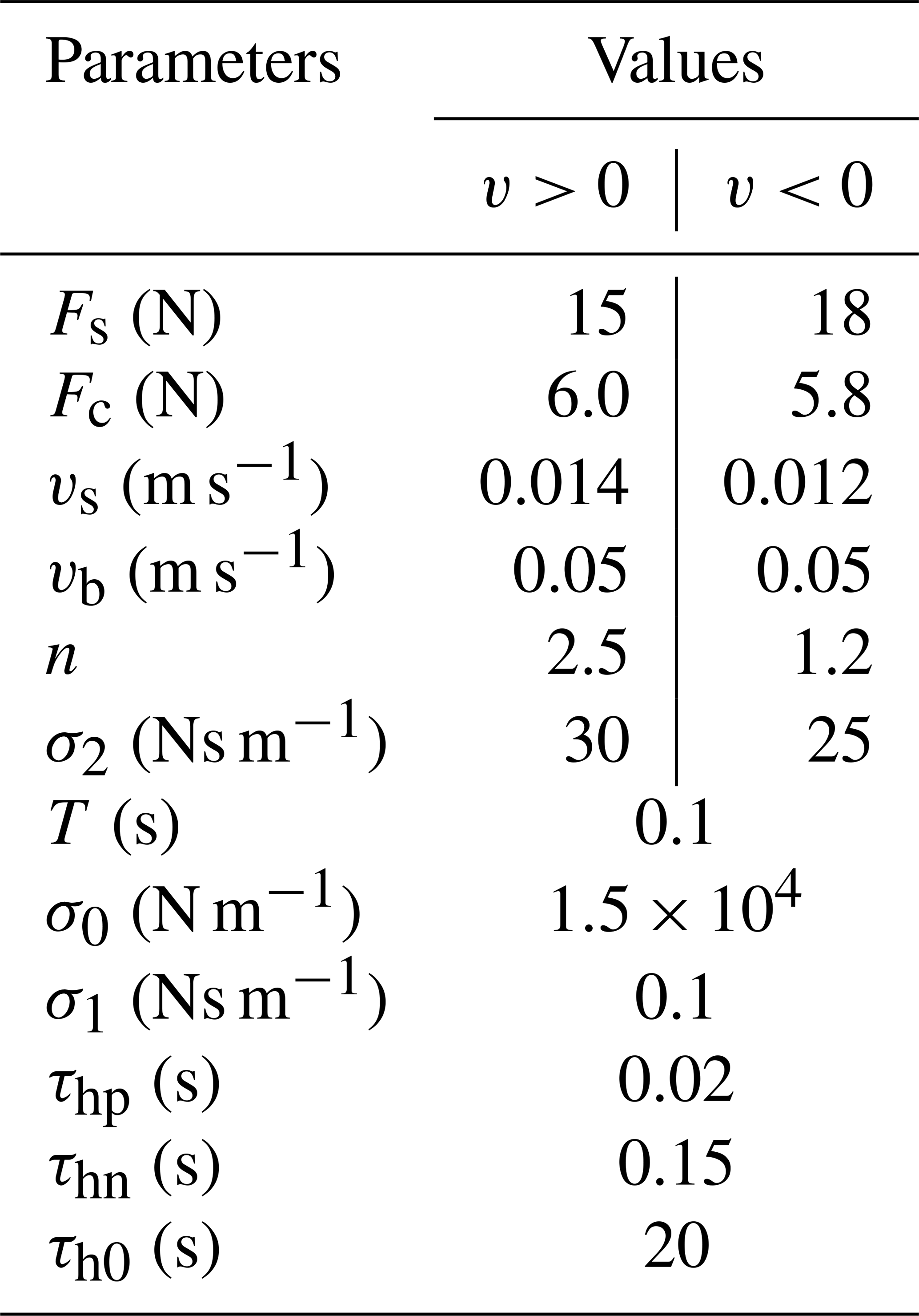
Figure 10 shows comparisons between the measured characteristics of the piston position, the pressures p1 in the cylinder chambers, the friction force and those simulated by the three friction models when low and constant voltage signals of the two proportional valves are supplied. It can realize in Fig. 10a that the stick-slip motion of the piston position can be relatively well predicted by the RLG model while the stick-slip motion can be partly predicted by the LG model; the number of stick-slip cycles of the piston motion predicted by the LG model are less than those by the RLG model. In addition, it is shown that the SS model cannot predict the stick-slip motion of the piston; the SS model can only create continue moving curves of the piston position and the pressures. In addition, much oscillation is observed in the friction force characteristic simulated by the SS model in Fig. 10c. Such these limitations of the SS model may be due to lack of the stiction characteristic combined in the model. These results obtained in Fig. 10 verify a better simulation capacity of the RLG model comparing to the LG model and the SS model when the piston is operated at low velocity range.
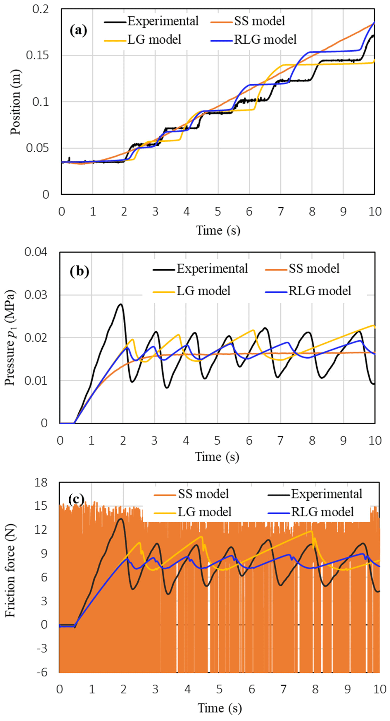
Figure 10Comparison between measured characteristics of the piston position, pressures and friction force and those simulated using the three friction models: (a) position, (b) pressure p1, (c) friction force (M=0.5 kg, u1=2.875 V, u2=2.19 V).
Figure 11 compares the measured characteristics of the piston position, the pressures p1 and p2 in the cylinder chambers, the friction force with those simulated by the three friction models at the following operating conditions of the valve signals: (V) and (V). The varying frequency of the valve signals was 0.2 Hz and the load mass was 0.5 kg. The comparison results show that both the RLG model and the LG model give the same simulation results and can simulate the measured characteristics with a relatively good accuracy. It is noted that in the RLG model the lubricant film dynamics is added into the LG model in order to simulate a decrease of the maximum friction force observed after one cycle of the velocity variation in a hydraulic cylinder. However, such this decrease of the maximum friction force cannot be observed experimentally in the pneumatic cylinder as shown in Figs. 9d and 11d. Therefore, the usefulness of the RLG model comparing to the LG model cannot be realized for the pneumatic cylinder when the piston is operated under sliding regime and under varied velocity conditions with reversal. For the simulated results of the SS model, it can realize that the SS model can also track well the measured position of the piston (Fig. 11a). However, the pressures and the friction force predicted by the SS model are much smaller than those of the measured ones. In addition, the SS model causes much oscillations at the stop intervals of the piston position in the friction force characteristic as shown in Fig. 11d.
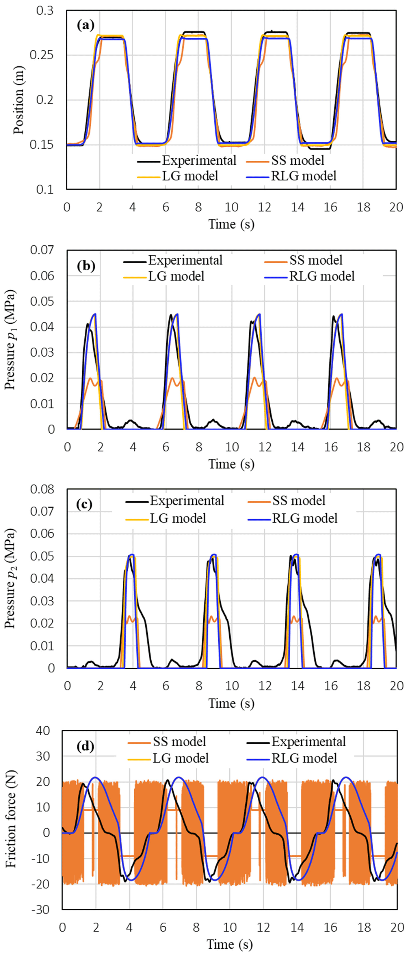
Figure 11Comparison between measured characteristics of the piston position, pressures and friction force and those simulated using the three friction models: (a) piston position, (b) pressure p1, (c) pressure p2, (d) friction force (M=0.5 kg, (V), (V), f=0.2 Hz).
Figure 12 show comparisons between the measured characteristics of the piston and those simulated by the three friction models when the voltage signals of the two proportional valves were varied by sinusoidal waves with a high frequency f=1 Hz. It shows that the same simulation results as obtained in Fig. 11 can be also achieved by the three friction models in Fig. 12. Therefore, the simulation results obtained from Figs. 10 to 12 verify that the RLG model is the best for the pneumatic cylinder in the three friction models considered in this study.
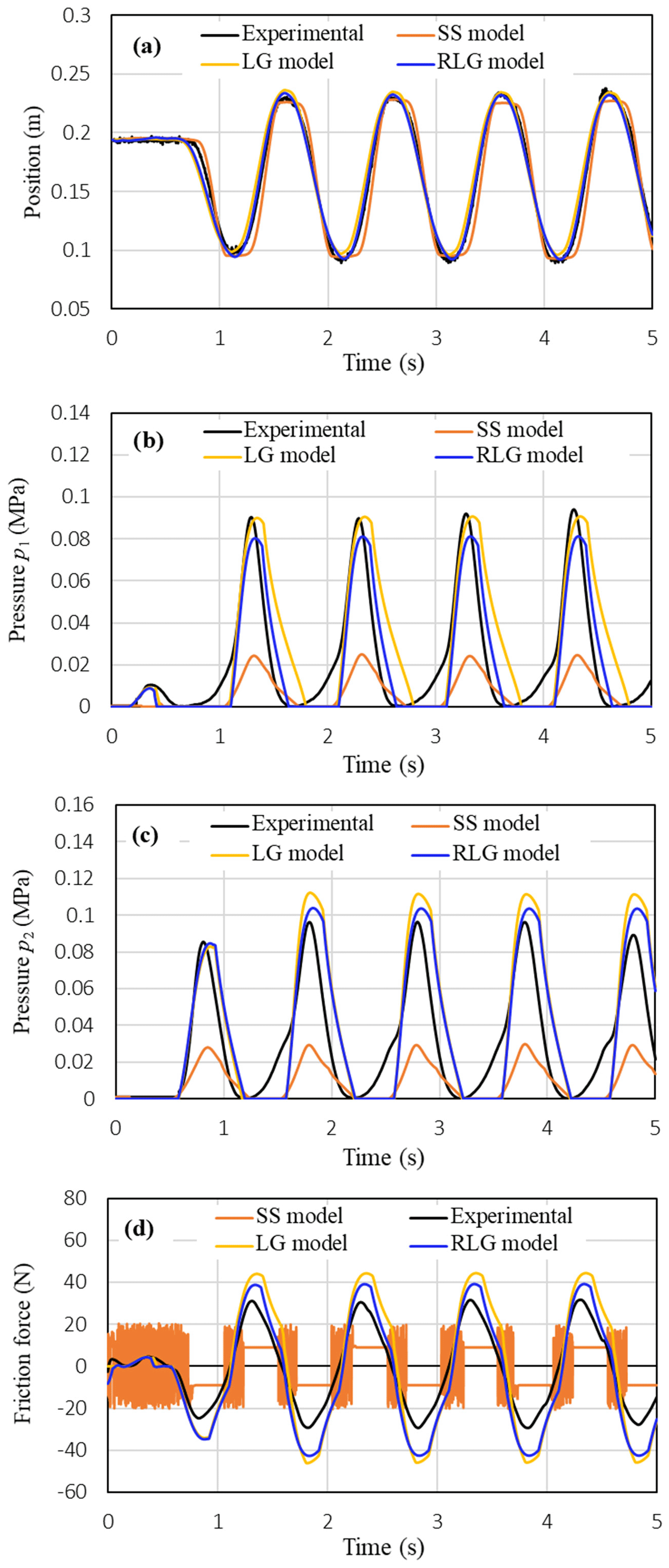
Figure 12Comparison between measured characteristics of the piston position, pressures and friction force and those simulated using the three friction models: (a) position, (b) pressure p1, (c) pressure p2, (d) friction force (M=0.5 kg, (V), (V), f=1 Hz).
In this study, both experiments and simulations were conducted to examine the effects of friction models on the simulation accuracy of an electro-pneumatic servo system. Three friction models: a SS model (static + Coulomb + viscous friction), the LG model and the RLG model were examined. The characteristics of the piston position, the piston velocity, the pressures in the cylinder chambers and the friction force under different operating conditions of the valve inputs were measured, analysed and used for verification of the friction models. It has been verified that the RLG model can give the best simulation results among the three friction models. The LG model give relatively good results except for a limitation in simulating the stick-slip motion of the piston at low velocity condition. It has been also verified that the steady-state fiction model used in this study is unable to simulate the stick-slip motion as well as causes much oscillation in the friction force characteristics. The application of the RLG model or the LG model to control of a servo pneumatic system with friction compensation will be the subject for a future research.
The data in this study can be requested from the corresponding author.
The supplement related to this article is available online at: https://doi.org/10.5194/ms-10-517-2019-supplement.
XBT and VLN designed the experiment and VLN carried it out. XBT and KDT developed the mathematical model of the system. VLN built the simulation code and performed the simulations. XBT prepared the manuscript with contributions from all co-authors.
The authors declare that they have no conflict of interest.
The authors would like to thank Huy Thuong Dao for his assistance in collecting the experimental data.
This research has been supported by the Hanoi University of Science and Technology (grant no. T2018-PC-042).
This paper was edited by Marek Wojtyra and reviewed by two anonymous referees.
Ahmed, F. S., Laghrouche, S., and Harmouche, M.: Adaptive backstepping output feedback control of DC motor actuator with friction and load uncertainty compensation, Int. J. Robust Nonlinear Control, 25, 1967–1992, https://doi.org/10.1002/rnc.3184, 2015.
Armstrong, H. B.: Control of machines with friction, Springer, Boston, https://doi.org/10.1007/978-1-4615-3972-8, 1991.
Armstrong, H. B., Dupont, P., and Canudas, D. W. C.: A survey of models, analysis tools and compensation methods for the control of machines with friction, Automatica, 30, 1083–1138, https://doi.org/10.1016/0005-1098(94)90209-7, 1994.
Brown, P. and McPhee, J.: A continuous velocity-based friction model for dynamics and control with physically meaningful parameters, J. Computa. Nonlin. Dyn., 11, 054502, https://doi.org/10.1115/1.4033658, 2016.
Canudas, D. W. C., Olsson, H., Åström, K. J., and Linschinsky, P.: A new model for control of systems with friction, IEEE T. Automat. Contr., 40, 419–425, https://doi.org/10.1109/9.376053, 1995.
Dupont, P. E.: Friction modeling and PD compensation at very low velocities, J. Dyn. Syst.-T. ASME, 117, 8–14, https://doi.org/10.1115/1.2798527, 1995.
Dupont, P., Hayward, V., Armstrong, B., and Altpeter, F.: Single state elastoplastic friction models, IEEE T. Automat. Contr., 47, 787–792, https://doi.org/10.1109/TAC.2002.1000274, 2002.
Freidovich, L., Robertsson, A., Shiriaev, A., and Johansson, R.: Lugre-model-based friction compensation, IEEE T. Contr. Syst. T., 18, 194–200, https://doi.org/10.1109/TCST.2008.2010501, 2010.
Green, P., Worden, K., and Sims, N.: On the identification and modelling of friction in a randomly excited energy harvester, J. Sound Vib., 332, 4696–4708, https://doi.org/10.1016/j.jsv.2013.04.024, 2013.
Haessig, D. A. and Friedland, B.: On the modeling of friction and simulation, J. Dyn. Syst.-T. ASME, 113, 354–362, https://doi.org/10.1115/1.2896418, 1991.
Hibi, A. and Ichikawa, T.: Mathematical model of the torque characteristics for hydraulic motors, B. JSME, 20, 616–621, https://doi.org/10.1299/jsme1958.20.616, 1977.
Hodgson, S., Le, M. Q., Tavakoli, M., and Pham, M. T.: Improved tracking and switching performance of an electropneumatic positioning system, Mechatronics 22, 1–12, https://doi.org/10.1016/j.mechatronics.2011.10.007, 2012.
Hoshino, D., Kamamichi, N., and Ishikawa, J.: Friction compensation using time variant disturbance observer based on the LuGre model, in: 12th IEEE International Workshop on Advanced Motion Control, IEEE, Sarajevo, Bosnia-Herzegovina, 25–27 March 2012, 1–6, 2012.
Lampaert, V., Al-Bender, F., and Swevers, J.: Experimental characterization of dry friction at low velocities on a developed tribometer setup for macroscopic measurements, Tribol. Lett., 16, 95–104, https://doi.org/10.1023/B:TRIL.0000009719.53083.9e, 2004.
Landolsi, F., Ghorbel, F. H., Lou, J., Lu, H., and Sun, Y.: Nanoscale friction dynamic modelling, J. Dyn. Syst.-T. ASME, 131, 061102, https://doi.org/10.1115/1.3223620, 2009.
Li, G., Zhang, C., Luo, J., Liu, S., Xie, G., and Lu X.: Film Forming Characteristics of Grease in Point Contact under Swaying Motions, Tribol. Lett., 35, 57–65, https://doi.org/10.1007/s11249-009-9433-7, 2009.
Lu, L., Yao, B., Wang, Q., and Chen, Z.: Adaptive robust control of linear motors with dynamic friction compensation using modified LuGre model, Automatica, 45, 2890–2896, https://doi.org/10.1016/j.automatica.2009.09.007, 2009.
Marques, F., Flores, P., Pimenta Claro, J. C., and Lankarani, H. M: A survey and comparison of several friction force models for dynamic analysis of multibody mechanical systems, Nonlinear Dynam., 86, 1407–1443, https://doi.org/10.1007/s11071-016-2999-3, 2016.
Marques, F., Flores, P., Claro, J. C. P., and Lankarani, H. M.: Modelling and analysis of friction including rolling effects in multibody dynamics: a review, Multibody Syst. Dyn., 45, 223–244, https://doi.org/10.1007/s11044-018-09640-6, 2019.
Mate, C. M., McClell, G. M., Erllandsson, R., and Chiang, S.: Atomic scale friction of a tungsten tip on a graphite surface, Phys. Rev. Lett., 59, 535–577, https://doi.org/10.1103/PhysRevLett.59.1942, 1987.
Peng, F. Q., Guo, L. T., Jian, F. C., and Bo, L.: Modelling and simulation of stick-slip motion for pneumatic cylinder based on meter-in circuit, Appl. Mech. Mater., 130, 775–780, https://doi.org/10.4028/www.scientific.net/AMM.130-134.775, 2012.
Pennestrì, E., Rossi, V., Salvini, P., and Valentini, P. P: Review and comparison of dry friction force models, Nonlinear Dynam., 83, 1785–1801, https://doi.org/10.1007/s11071-015-2485-3, 2016.
Piatkowski, T. and Wolski, M.: Analysis of selected friction properties with the Froude pendulum as an example, Mech. Mach. Theory, 119, 37–50, https://doi.org/10.1016/j.mechmachtheory.2017.08.016, 2018.
Sakiichi, O., Yoshitsugu, K., Michio, M., and Yasuo, Y.: Stick-slip Motion of Pneumatic Cylinder, Journal of the Japan Society for Precision Engineering, 54, 183–188, https://doi.org/10.2493/jjspe.54.183, 1988.
Sugimura, J., Jones, W. R., and Spikes, H. A.: EHD Film Thickness in Non-Steady State Contacts, J. Tribol., 120, 442–453, https://doi.org/10.1115/1.2834569, 1998.
Swevers, J., Al-Bencer, F., Ganseman, C.G., and Prajogo, T.: An integrated friction model structure with improved presiding behavior for accurate friction compensation, IEEE T. Automat. Contr., 45, 675–686, https://doi.org/10.1109/9.847103, 2000.
Tran, X. B. and Yanada, H.: Dynamic friction behaviors of pneumatic cylinders, Lect. Notes Contr. Inf., 4, 180–190, https://doi.org/10.4236/ica.2013.42022, 2013.
Tran, X. B., Hafizah, N., and Yanada, H.: Modeling of dynamic friction behaviors of hydraulic cylinders, Mechatronics, 22, 65–75, https://doi.org/10.1016/j.mechatronics.2011.11.009, 2012.
Tran, X. B., Khaing, W. H., Endo, H., and Yanada, H.: Effect of friction model on simulation of hydraulic actuator, P. I. Mech. Eng. I-J. Sys., 228, 690–698, https://doi.org/10.1177/0959651814539476, 2014.
Tran, X. B., Dao, H. T., and Tran, K. D.: A new mathematical model of friction for pneumatic cylinders, P. I. Mech. Eng. C-J. Mec., 230, 2399–2412, https://doi.org/10.1177/0954406215594828, 2016.
Tressler, J. M., Clement, T., Kazerooni, H., and Lim, M.: Dynamic behavior of pneumatic systems for lower extremity extenders, in: Proceedings of the 2002 IEEE International Conference on Robotics & Automation, IEEE, Washington DC, 11–15 May 2002, 3248–3253, 2002.
Wojtyra, M.: Comparison of two versions of the LuGre model under conditions of varying normal force, in: Proceedings of the 8th ECCOMAS Thematic Conference on Multibody Dynamics 2017, Nakladatelstvi CVUT (CTN), Prague, Czechia, 19–22 June 2017, 335–344, 2017.
Yanada, H. and Sekikawa, Y.: Modeling of dynamic behaviors of friction, Mechatronics, 18, 330–339, https://doi.org/10.1016/j.mechatronics.2008.02.002, 2008.