Kinematic and dynamic modeling of a novel 4-degree-of-freedom parallel mechanism

In this paper, a novel 4-degree-of-freedom (DOF) parallel mechanism (PM) limb is proposed. The properties of the degrees of freedom are verified based on the screw theory. The inverse position, velocity, and acceleration models of the mechanism are developed. The position workspace of the mechanism is generated based on the inverse kinematic model. The singular configurations are identified within the workspace. The distribution of the stiffness index in the workspace is visualized. The inverse dynamic model of the mechanism is developed based on the Lagrangian method. The kinematic and dynamic simulations of the mechanism are carried out in Adams to verify the correctness of the theoretical model. Most of the kinematic joints of the mechanism are revolute joints and form the sub-closed-loop parallelogram structure, which makes this mechanism exhibit promising application prospects for application in high-speed or heavy-load fields.

1 Introduction

The mechanism is the skeleton of mechanical equipment and the key to determining its working performance. As one of the significant branches of the mechanism family, the parallel mechanism (PM) has made tremendous contributions to the development of the equipment-manufacturing industry since its birth due to its distinctive structural, kinematic, and mechanical characteristics (Kucuk, 2018; Ebrahimi et al., 2018; Ye et al., 2020). There are many kinds of PMs, which can be divided into 6-degree-of-freedom (DOF) PMs and lower-mobility PMs in terms of DOFs (Chong et al., 2020; Gan et al., 2016; Isaksson and Watson, 2013). In the early stage of PM applications, 6-DOF parallel devices are adopted in some production operations that require only low mobility, which leads to problems such as large equipment volume, high manufacturing cost, and complex control systems (Gan et al., 2016; Ye and Li, 2019; Ye et al., 2017). For these reasons, it has become a problem of great concern to mechanism researchers whether the DOFs of parallel devices can be matched to the motion dimensions of the task and/or whether they can be equal to the DOFs of the equipment when executing tasks that require fewer than 6 DOFs. Therefore, the concept of a lower-mobility PM is proposed, and lower-mobility PMs have been widely studied (Sun and Huo, 2018; Shen et al., 2020; Liu et al., 2019).

Lower-mobility PMs refer to PMs with 2–5 DOFs (Zeng et al., 2011). The lower-mobility PMs have a simple structure, a large workspace-to-volume ratio, and a simple control system compared to the 6-DOF PMs. Therefore, they have good application prospects in high-speed sorting, footed mobile robots, rehabilitation medicine, machining, and wave power generation (Chang and Zhang, 2019; Tian et al., 2020; Yang et al., 2018). A number of lower-mobility PMs have been proposed so far. For example, Hunt proposed a variety of PMs with lower mobility based on the screw theory (Hunt, 1983). Cao et al. (2019) proposed a new 2-DOF PM and conducted its kinematic analysis (Cao et al., 2019). Tsai and Joshi developed a 3-DOF PM and carried out its forward and inverse kinematic analyses and structural optimization (Tsai and Joshi, 2000). Gao et al. (2015) studied a class of 4-DOF PMs based on the generalized-function (G_F) set-based synthesis (He et al., 2015). Lu et al. put forward a 5-DOF PM and derived the formulas for solving displacement, velocity, acceleration, and dynamic driving forces (Lu et al., 2018).

Among the many lower-mobility PMs, the 4-DOF PMs with three translations and one rotation (3T1R) have a large workspace at their end effectors and have garnered considerable attention in material handling, express sorting, palletizing, and so on (Xu et al., 2017; Arian et al., 2020; Pakzad et al., 2019). However, most of the existing 4-DOF PMs with 3T1R employ a single open-chain limb configuration. For instance, typical examples include the 4-UPU PM, 4-PRRU (Quadrupteron) PM, PRRR-3PRRS (TetraFLEX) PM, and 3UPU-PRRR PM (Huang and Li, 2003; Richard et al., 2007; Simas et al., 2022; Amine et al., 2017). Due to the parallelogram structures in their limbs, these PMs have lower rigidity and a lower maximum operating speed compared with the Delta and H4 parallel robots (Pierrot and Company, 1999; Pierrot et al., 2001). The limb mass of such PMs with a single open chain is large at the same stiffness level, resulting in poor dynamic performance, thus limiting their applicability in high-speed, heavy-load, and high-precision operations. Currently, many scholars are committed to developing lower-mobility PMs with sub-closed-loop structures in their limbs to promote the application of PMs in the mechanical-manufacturing field.

Most studies of PMs with 3T1R have focused on the PMs with three joints in a limb, with research covering their forward and inverse kinematics, workspace analysis, singularity analysis, and dynamic characteristics (Arian et al., 2020; Isaksson et al., 2017). Xie and Liu (2015) proposed a novel R(Pa*)R PM (X4), for which they conducted optimal design and workspace identification (where Pa* denotes a composite parallelogram mechanism) (Xie and Liu, 2015). Zhang et al. (2019) established the forward and inverse position models and analyzed the singular configurations of the 4-URU PM and obtained its workspace (Zhang et al., 2019). Zarkandi carried out forward and inverse dynamic analyses of a 4RSS + PS manipulator (Zarkandi et al., 2019). Wang established the dynamic model of the 4-SPS/CU PM (where C denotes a cylindrical joint) (Wang, 2018).

In contrast, research on the dynamics of PMs with 3T1R and four-joint sub-closed-loop limbs remains scarce. Dynamic analysis is essential for actuator selection, precision control of the mechanism, mechanical vibration analysis, and dynamic optimization and plays a crucial role in practical applications (Pakzad et al., 2019). Due to the multiple links and sub-closed-loop chains in PMs, the dynamic analysis of such PMs with 3T1R and four-joint sub-closed-loop passive limbs poses greater challenges. The dynamic study of PM with 3T1R can refer to studies on parallel mechanisms with other motion characteristics. For example, Sun et al. (2024) studied dynamic modeling and performance analysis of the 2PRU-PUU reconfigurable parallel mechanism. Yuan et al. (2024) established the electro-hydraulic-driven 3-UPS/S parallel stabilization platform dynamic equation using the virtual-work principle. Taking the bio-inspired masticatory parallel mechanism as an example, Cheng et al. (2024) built an inverse dynamic model by virtue of a dynamic method and derived the Hessian matrices of the constraint equations. Russo et al. (2024) reviewed several dynamic analysis methods for parallel machine tools. Liang et al. (2024) established the dynamic model by means of the Lagrangian method, and the effectiveness of the model is verified via Adams software.

In this paper, a novel 4-DOF PM with the 3-RPaPaR limbs is proposed (where Pa denotes a parallelogram joint). The properties of the degrees of freedom are verified based on the screw theory. The kinematic modeling is dealt with. The workspace is studied based on the inverse kinematic model. The singular configurations are described within the workspace. The distribution of the stiffness index is analyzed. The inverse dynamic model is developed based on the Lagrangian method. The correctness of kinematic and dynamic theoretical models is verified by simulation in Adams.

2 Mechanism description

A novel 4-DOF PM with the 3-RPaPaR limb is proposed in this paper, as illustrated in Fig. 1. The PM consists of a base, a moving platform, and three limbs. The limb^1st is composed of the actuated limb^1st, the actuated limb^4th, and the passive limb^1st. The limb^2nd consists of the actuated limb^2nd and the passive limb^2nd. The limb^3rd is composed of the actuated limb^3rd and the passive limb^3rd.

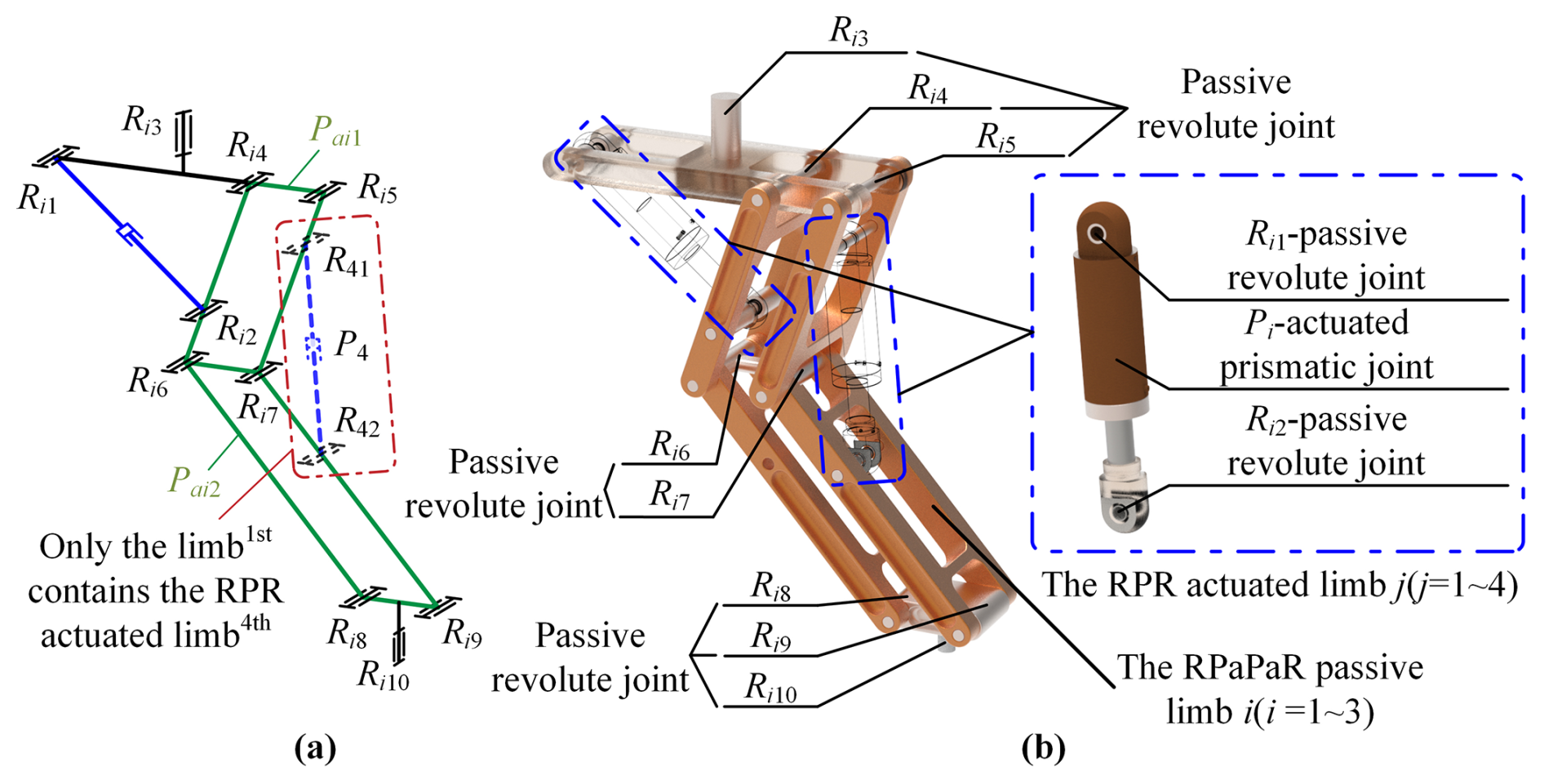
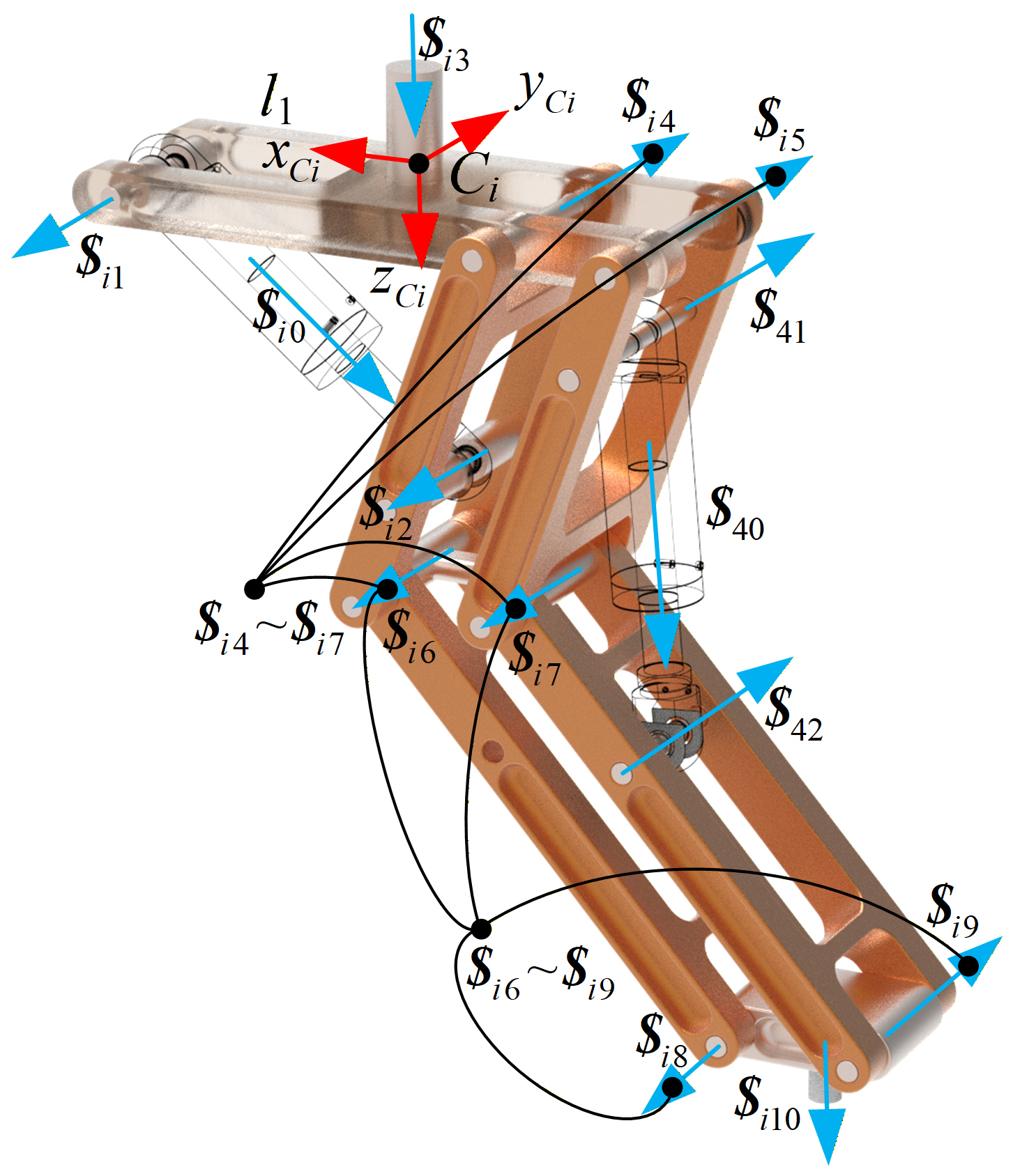
In the mechanism, all of the actuated limbs are based on the RPR limb configuration, and the prismatic joint (P) serves as the actuated joint. All passive limbs are based on the RPaPaR limb, and R_i4–R_i7 form the parallelogram joint P_ai1, and R_i6–R_i9 form the parallelogram joint P_ai2. R_i3 and R_i10 denote the revolute joints connecting the passive limb to the base and the moving platform, respectively. The rotational axes of R_i3 and R_i10 are parallel to each other and perpendicular to the base, while the axes of the other revolute joints are parallel to the base, as illustrated in Fig. 2.

Figure 1 The CAD model of a novel 4-DOF PM.

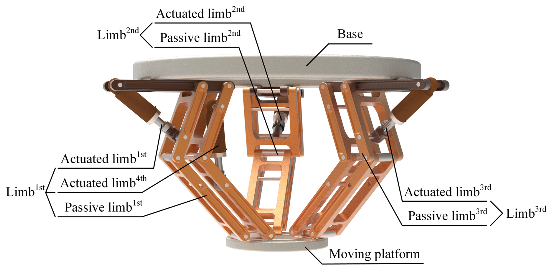
The actuated prismatic joint is placed between the passive limb links to improve actuation efficiency and the output force and torque of this PM. The passive limbs are composed entirely of revolute joints (R) as revolute joints feature easy manufacturing, high precision, and low cost. In comparison with the open-chain configuration, the closed-loop configuration enhances the structural stiffness of the mechanism. This configuration also ensures that the moving platform remains consistently parallel to the base. In comparison with traditional 4-DOF PMs, with the limb comprising two links and three joints, the RPaPaR passive limb is equivalent to a structure with three links and four joints. Therefore, the proposed PM offers a larger workspace. Meanwhile, the PM with three limbs exhibits superior acceleration performance compared to those with four limbs due to its simpler structural design and lower overall mass.

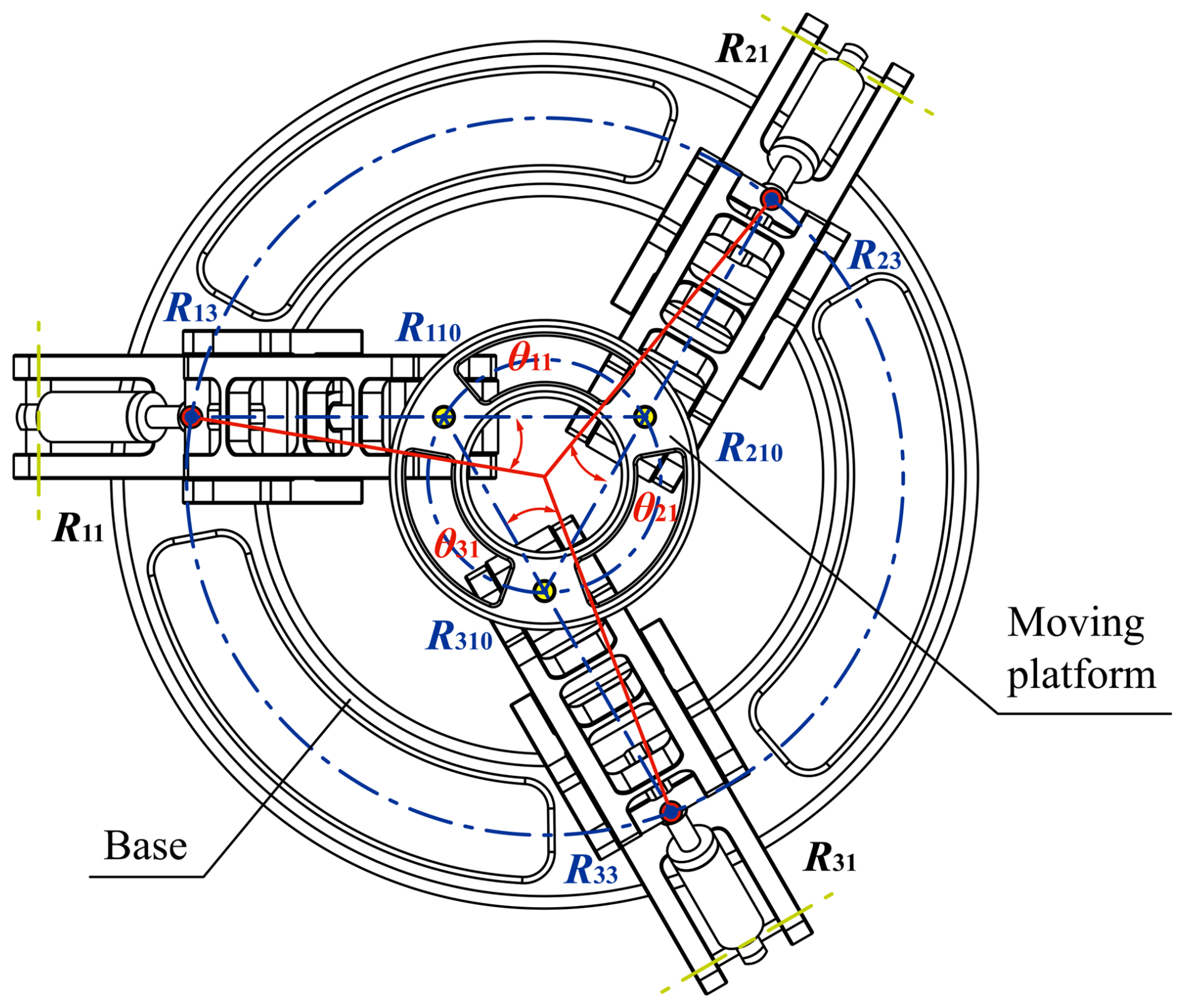
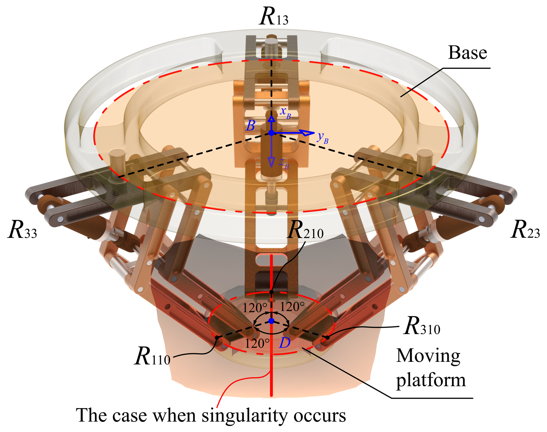
A bottom view of the mechanism is presented in Fig. 3. Notably, the R_i3 joints are uniformly distributed on a circular path on the base, and the R_i10 joints are similarly distributed on a circular path on the moving platform. In a general configuration, the angle θ_i1 between the limb plane and the line connecting the base to the R_i3 joint is not equal to 0° (θ_i1≠0°). If θ_i1 is equal to 0°, the mechanism will experience a malfunction.

Figure 2 The ith limb: (a) kinematic scheme and (b) CAD model.

Figure 3 The bottom view of the novel 4-DOF PM.

3 Kinematic analysis

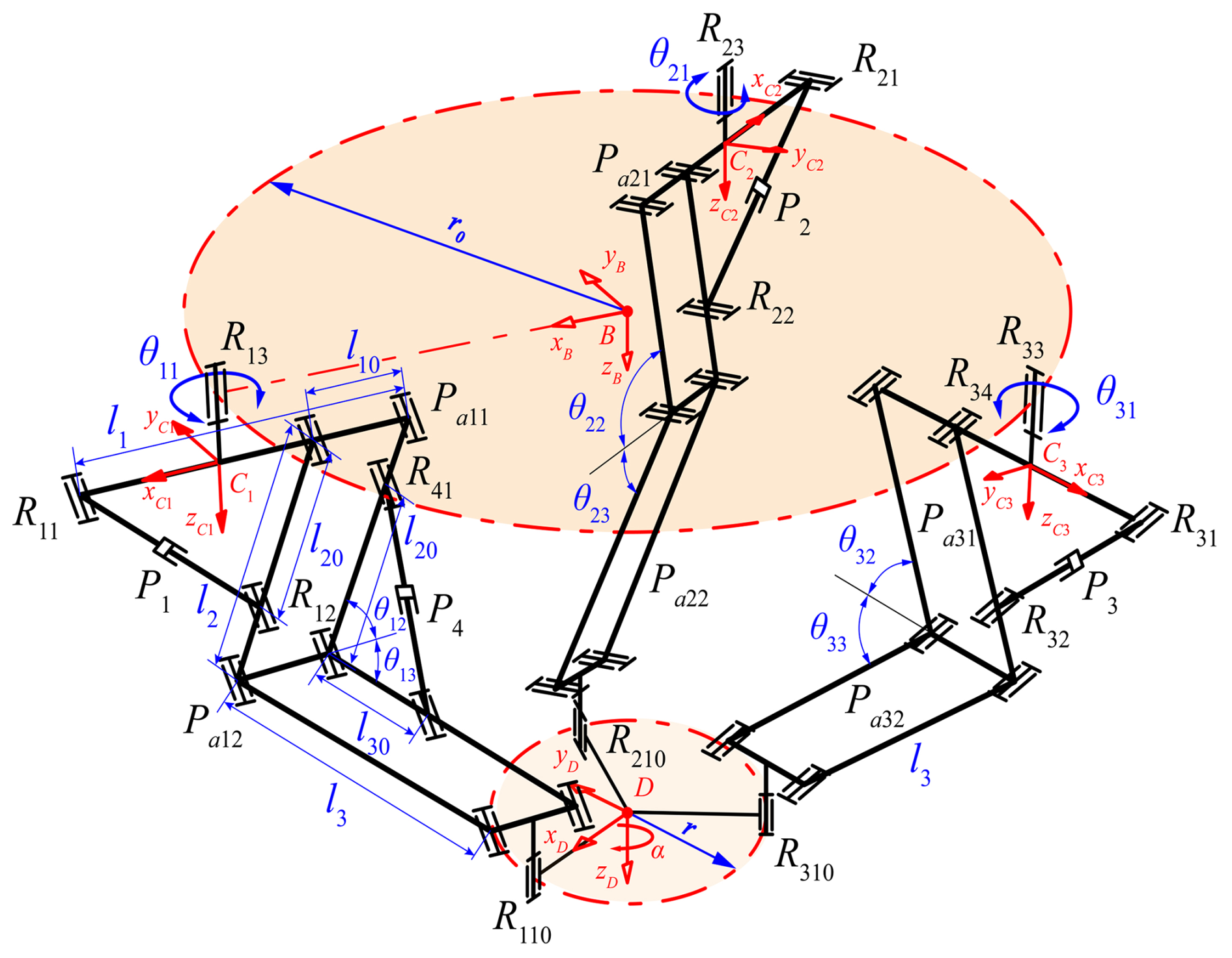
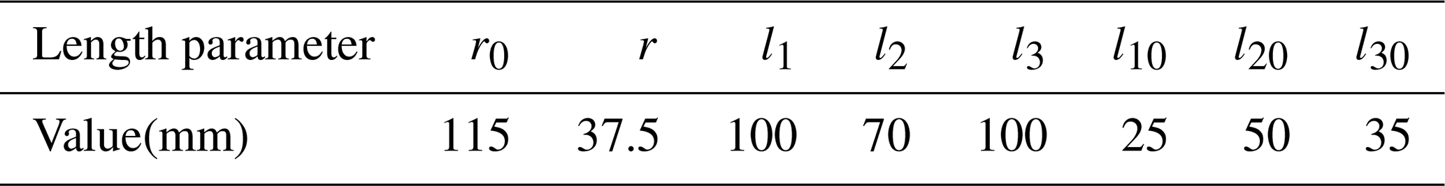
As illustrated in Fig. 4, the base frame {B}: B−x_By_Bz_B is attached to the center point B of the base. The moving frame {D}: D−x_Dy_Dz_D is attached to the center point D of the moving platform. Moreover, the link frame {C_i}: $C_i-x_{C_i}{y}_{C_i}{z}_{C_i}$ (i=1–3) is attached to the center point C_i of the link R_i1R_i5. The x_B-axis direction is from point B to point R₁₃ on the base, the x_D axis is from point D to R₁₁₀ on the moving platform, the $x_{C_i}$ axis is from point C_i to R_i1, all of the z axes are vertically downward, and all of the y axes are determined through the right-hand rule. The point R_i3 coincides with the center point C_i of link R_i1R_i5, and point R_i10 coincides with the center of link R_i8R_i9. The length and angle parameters of the PM are shown in Fig. 4. We define θ_i0 as the angle between BC_i and x_B.

Figure 4 The kinematic scheme of the novel 4-DOF PM.

3.1 Verification of DOF

Analysis of the motion characteristics of the end effector is a core step in the research of PMs. In this paper, the degrees of freedom of the mechanism are calculated and verified using screw theory. The first limb is selected as the research object for analysis, and the screw representation of the first limb is shown in Fig. 5.

Figure 5 Schematic diagram of screw of the limb.

In this paper, the screws of each kinematic pair for all limbs are first given, and then the reciprocal screws of the mechanism, i.e., the constraint screws, are solved. By performing secondary reciprocal screw solving, the DOF characteristics of the end effector of the mechanism are derived.

The screws of kinematic pairs P_i, R_i1–R_i3, R_i10, and R₄₁ and R₄₂ correspond to _i0, _i1–_i3, _i10, and ₄₁ and ₄₂, respectively. Both R_i4–R_i7 and R_i6–R_i9 are equivalent to parallelogram hinges, whose corresponding screws are _i4– _i7 and _i6– _i9. In the coordinate system {C₁}: C₁–$x_{C_{\mathrm{1}}}{y}_{C_{\mathrm{1}}}{z}_{C_{\mathrm{1}}}$, the motion screws of the first limb, including the driving chain and the executing chain, are expressed as follows:

$$\begin{array}{}\text{(1)}& \textcolor{red}{}\end{array}$$

where d, e, and f are all real numbers.

From Eq. (1), the reciprocal screw of the first limb is derived as

$$\begin{array}{}\text{(2)}& \textcolor{red}{}\end{array}$$

Similarly, the second and third limbs do not contain ₄₀, ₄₁, and ₄₂. The reciprocal screws of the second and third limbs in the coordinate systems {C₂}: $C_{\mathrm{2}}-x_{C_{\mathrm{2}}}{y}_{C_{\mathrm{2}}}{z}_{C_{\mathrm{2}}}$ and {C₃}: $C_{\mathrm{3}}-x_{C_{\mathrm{3}}}{y}_{C_{\mathrm{3}}}{z}_{C_{\mathrm{3}}}$ can be derived in the same way.

$$\begin{array}{}\text{(3)}& \textcolor{red}{}\end{array}$$

Each limb applies a constraint couple on the moving platform. These three constraint couples are perpendicular to the revolute pairs R₁₁₀, R₂₁₀, and R₃₁₀ respectively, and all lie parallel to the plane of the moving platform. On this basis, in the coordinate system {D} D−x_Dy_Dz_D, the constraint screw system of the moving platform (containing three screws) can be expressed as

$$\begin{array}{}\text{(4)}& \textcolor{red}{}\end{array}$$

where j and k are real numbers.

Since these three screws are linearly dependent, they only correspond to two independent constraints, with one being a redundant constraint. Their second reciprocal screws ^rr are exactly the motion screws of the moving platform, which are used to determine the DOF characteristics of the mechanism.

$$\begin{array}{}\text{(5)}& \textcolor{red}{}\end{array}$$

According to the motion screws of the moving platform, it can be determined that the moving platform has four DOFs, specifically three translational DOFs and one rotational DOF about the Z axis. During the motion process of the mechanism, the above constraint screws remain unchanged. The over-constraints of the mechanism include common constraints and redundant constraints: the number of common constraints is 0, the number of redundant constraints is always 1, and the mechanism has full-cycle DOFs.

3.2 Position analysis

Let χ=[D^Tα]^T be the position and orientation vector of point D in {B}, where D = [X Y Z]^T, and α is the angle of rotation of {D} about the z_B axis. θ_i0 is the angle between the $x_{C_i}$ axis and x_B axis. Let L_i (i=1–3) and L₄ be the length of vectors R_i1R_i2 and R₄₁R₄₂. The position analysis is the process of solving L=[L₁L₂L₃L₄]^T with known χ.

Let ${}_D^B\mathbf{T}$ and ${}_{Ci}^B\mathbf{T}$ (i = 1–3) be the homogeneous transformation matrixes from {D} to {B} and from {C_i} to {B}, respectively; they can be expressed as follows:

$$\begin{array}{}\text{(6)}& {}_D^B\mathbf{T}=\left[\begin{array}{cc}{}_D^B\mathit{R}& \mathit{D}\\ {\mathbf{0}}_{\mathrm{1}\times \mathrm{3}}& \mathrm{1}\end{array}\right],{}_{C_i}^B\mathbf{T}=\left[\begin{array}{cc}{}_{C_i}^B\mathit{R}& {}^B{\mathit{C}}_i\\ {\mathbf{0}}_{\mathrm{1}\times \mathrm{3}}& \mathrm{1}\end{array}\right],\end{array}$$

where ${}_D^B\mathbf{R}$ and ${}_{Ci}^B\mathbf{R}$ (i = 1–3) denote the rotation matrixes from {D} to {B} and from {C_i} to {B}, respectively; they can be expressed as follows:

$$\begin{array}{}\text{(7)}& {}_D^B\mathbf{R}={\mathbf{R}}_z\left(\mathit{\alpha }\right),{}_{C_i}^B\mathbf{R}={\mathbf{R}}_z\left({\mathit{\theta }}_{i\mathrm{0}}\right){\mathbf{R}}_z\left({\mathit{\theta }}_{i\mathrm{1}}\right),\end{array}$$

where R_z(^∗) can be written as

$$\begin{array}{}\text{(8)}& {\mathbf{R}}_z(\ast )=\left[\begin{array}{ccc}{\mathrm{c}}^{\ast }& -{\mathrm{s}}^{\ast }& \mathrm{0}\\ {\mathrm{s}}^{\ast }& {\mathrm{c}}^{\ast }& \mathrm{0}\\ \mathrm{0}& \mathrm{0}& \mathrm{1}\end{array}\right],\end{array}$$

where s and c denote sin and cos, respectively.

^BC_i (i=1–3) denotes the position vector of point C_i in {B} as follows:

$$\begin{array}{}\text{(9)}& {}^B{\mathit{C}}_i={\mathbf{R}}_z\left({\mathit{\theta }}_{i\mathrm{0}}\right)\left[\begin{array}{c}{r}_{\mathrm{0}}\\ \mathrm{0}\\ \mathrm{0}\end{array}\right]=\left[\begin{array}{c}{r}_{\mathrm{0}}\mathrm{c}{\mathit{\theta }}_{i\mathrm{0}}\\ r_{\mathrm{0}}\mathrm{s}{\mathit{\theta }}_{i\mathrm{0}}\\ \mathrm{0}\end{array}\right].\end{array}$$

^BR_i10 and ^DR_i10 (i=1–3) express the position vectors of point R_i10 in {B} and {D}, respectively; the mathematical relationship between them is

$$\begin{array}{}\text{(10)}& \begin{array}{rl}\left[\begin{array}{c}{}^B{\mathit{R}}_{i\mathrm{10}}\\ \mathrm{1}\end{array}\right]& ={}_D^B\mathbf{R}\left[\begin{array}{c}{}^D{\mathit{R}}_{i\mathrm{10}}\\ \mathrm{1}\end{array}\right]\\ & =\left[\begin{array}{c}{}^D{\mathit{R}}_{i\mathrm{10}x}\mathrm{c}\mathit{\alpha }-{}^D{\mathit{R}}_{i\mathrm{10}y}\mathrm{s}\mathit{\alpha }+X\\ {}^D{\mathit{R}}_{i\mathrm{10}x}\mathrm{s}\mathit{\alpha }+{}^D{\mathit{R}}_{i\mathrm{10}y}\mathrm{c}\mathit{\alpha }+Y\\ Z\\ \mathrm{1}\end{array}\right],\end{array}\end{array}$$

where ^DR_i10 (i=1–3) is expressed as follows:

$$\begin{array}{}\text{(11)}& {}^D{\mathit{R}}_{i\mathrm{10}}=\left[\begin{array}{c}{}^D{\mathit{R}}_{i\mathrm{10}x}\\ {}^D{\mathit{R}}_{i\mathrm{10}y}\\ {}^D{\mathit{R}}_{i\mathrm{10}z}\end{array}\right]=R_z\left({\mathit{\theta }}_{i\mathrm{0}}\right)\left[\begin{array}{l}r\\ \mathrm{0}\\ \mathrm{0}\end{array}\right]=\left[\begin{array}{c}r\mathrm{c}{\mathit{\theta }}_{i\mathrm{0}}\\ r\mathrm{s}{\mathit{\theta }}_{i\mathrm{0}}\\ \mathrm{0}\end{array}\right].\end{array}$$

^CiR_i10 (i=1–3) expresses the position vectors of point R_i10 in {C_i}. The mathematical relationship between ^BR_i10 and ^CiR_i10 is

$$\begin{array}{}\text{(12)}& \begin{array}{rl}\left[\begin{array}{c}{}^B{\mathit{R}}_{i\mathrm{10}}\\ \mathrm{1}\end{array}\right]& ={}_{C_i}^B\mathit{T}\left[\begin{array}{c}{}^{C_i}{\mathit{R}}_{i\mathrm{10}}\\ \mathrm{1}\end{array}\right]\\ & =\left[\begin{array}{c}{a}_{i\mathrm{1}}^{C_i}{\mathit{R}}_{i\mathrm{10}x}+r_{\mathrm{0}}c{\mathit{\theta }}_{i\mathrm{0}}\\ a_{i\mathrm{2}}^{C_i}{\mathit{R}}_{i\mathrm{10}x}+r_{\mathrm{0}}s{\mathit{\theta }}_{i\mathrm{0}}\\ {}^{C_i}{\mathit{R}}_{i\mathrm{10}z}\\ \mathrm{1}\end{array}\right],\end{array}\end{array}$$

where ${}^{C_i}$R_i10, α_i1, and α_i2 (i=1–3) are expressed as follows:

$$\begin{array}{}\text{(13)}& {\displaystyle }\begin{array}{rl}{}^{C_i}{\mathit{R}}_{i\mathrm{10}}& =\left[\begin{array}{c}{}^{C_i}{\mathit{R}}_{i\mathrm{10}x}\\ {}^{C_i}{\mathit{R}}_{i\mathrm{10}y}\\ {}^{C_i}{\mathit{R}}_{i\mathrm{10}z}\end{array}\right]\\ & =\left[\begin{array}{c}-l_{\mathrm{1}}/\mathrm{2}+l_{\mathrm{10}}/\mathrm{2}+l_{\mathrm{2}}c{\mathit{\theta }}_{i\mathrm{2}}-l_{\mathrm{3}}c{\mathit{\theta }}_{i\mathrm{3}}\\ \mathrm{0}\\ l_{\mathrm{2}}s{\mathit{\theta }}_{i\mathrm{2}}+l_{\mathrm{3}}s{\mathit{\theta }}_{i\mathrm{3}}\end{array}\right],\end{array}\text{(14)}& {\displaystyle }{a}_{i\mathrm{1}}=c{\mathit{\theta }}_{i\mathrm{0}}c{\mathit{\theta }}_{i\mathrm{1}}-s{\mathit{\theta }}_{i\mathrm{0}}s{\mathit{\theta }}_{i\mathrm{1}},a_{i\mathrm{2}}=c{\mathit{\theta }}_{i\mathrm{0}}s{\mathit{\theta }}_{i\mathrm{1}}+s{\mathit{\theta }}_{i\mathrm{0}}c{\mathit{\theta }}_{i\mathrm{1}}.\end{array}$$

Based on Eqs. (10) and (12), θ_ij (i=1–3; j=2, 3) can be obtained as follows (Ayiz and Kucuk, 2009; Kucuk and Gungor, 2016):

$$\begin{array}{}\text{(15)}& \begin{array}{rl}{\mathit{\theta }}_{ij}& =\arcsin \mathrm{2}\left(a_{i\mathrm{3}}-c_j(l_{\mathrm{2}}^{\mathrm{2}}-l_{\mathrm{3}}^{\mathrm{2}}),\mathrm{2}{l}_j\sqrt{a_{i\mathrm{3}}}\right)\\ & -c_j\arctan \mathrm{2}\left(a_{i\mathrm{4}},Z\right),\end{array}\end{array}$$

where α_i3 and α_i4(i=1–3) are expressed as

$$\begin{array}{}\text{(16)}& \begin{array}{rl}& a_{i\mathrm{3}}=a_{i\mathrm{4}}^{\mathrm{2}}+Z^{\mathrm{2}},a_{i\mathrm{4}}=\\ & \sqrt{X^{\mathrm{2}}+Y^{\mathrm{2}}+r^{\mathrm{2}}+r_{\mathrm{0}}^{\mathrm{2}}-\mathrm{2}r{r}_{\mathrm{0}}\mathrm{c}\mathit{\alpha }+c_{i\mathrm{0}}{a}_{i\mathrm{5}}}-(l_{\mathrm{1}}-l_{\mathrm{10}})/\mathrm{2},\end{array}\end{array}$$

$$\begin{array}{}\text{(17)}& a_{i\mathrm{5}}=-r\left[\mathrm{c}\mathit{\alpha }-{\displaystyle \frac{r_{\mathrm{0}}}{r}}s\mathit{\alpha }\right]{\mathbf{B}}_{i\mathrm{0}}\mathit{\chi },{\mathbf{B}}_{i\mathrm{0}}=\left[\begin{array}{l}\mathrm{1}\sqrt{\mathrm{3}}{c}_i\mathrm{0}\mathrm{0}\\ -\sqrt{\mathrm{3}}{c}_i\mathrm{1}\mathrm{0}\mathrm{0}\end{array}\right],\end{array}$$

where c₁=0, $c_{\mathrm{2}}=-\mathrm{1}$, c₃=1, $c_{\mathrm{10}}=-\mathrm{2}$, and $c_{\mathrm{20}}=c_{\mathrm{30}}=\mathrm{1}$.

In triangle R_i1R_i2R_i4 (i=1–3) and triangle R₄₁R₄₂R₁₇, L = [L₁ L₂L₃L₄]^T can be solved based on the cosine theorem as follows:

$$\begin{array}{}\text{(18)}& L_i=\sqrt{c_{i\mathrm{1}}^{\mathrm{2}}+l_{\mathrm{20}}^{\mathrm{2}}-\mathrm{2}{c}_{i\mathrm{1}}{l}_{\mathrm{20}}c{\mathit{\theta }}_{i\mathrm{2}}},(i=\mathrm{1}-\mathrm{4}),\end{array}$$

where $c_{\mathrm{11}}=c_{\mathrm{21}}=c_{\mathrm{31}}=l_{\mathrm{1}}$–l₁₀, c₄₁=l₃₀, and ${\mathit{\theta }}_{\mathrm{42}}={\mathit{\theta }}_{\mathrm{12}}+{\mathit{\theta }}_{\mathrm{13}}$.

3.3 Velocity analysis

Let $\dot{\mathit{\chi }}=$ [${\dot{\mathit{D}}}^{\mathrm{T}}\dot{\mathit{\alpha }}$]^T be the linear and angular velocity vector of point D in {B}, with $\dot{\mathit{D}}=$ [$\dot{X}$ $\dot{Y}\dot{Z}$]^T. Let V_i (i=1–3) and V₄ be the velocity of prismatic joint P_i and P₄, respectively. The velocity analysis is the process of solving V = [V₁V₂V₃V₄]^T with known $\dot{\mathit{\chi }}$.

By differentiating Eq. (18) with respect to time, the relationship between the velocity of the prismatic joint and ${\dot{\mathit{\theta }}}_{i\mathrm{2}}$ is derived as follows:

$$\begin{array}{}\text{(19)}& \begin{array}{rl}\mathbf{V}& ={\left[a_{\mathrm{16}}{\dot{\mathit{\theta }}}_{\mathrm{12}}{a}_{\mathrm{26}}{\dot{\mathit{\theta }}}_{\mathrm{22}}{a}_{\mathrm{36}}{\dot{\mathit{\theta }}}_{\mathrm{32}}{a}_{\mathrm{46}}{\dot{\mathit{\theta }}}_{\mathrm{42}}\right]}^{\mathrm{T}}\\ a_{i\mathrm{6}}& ={\displaystyle \frac{c_{i\mathrm{1}}{l}_{\mathrm{20}}\mathrm{s}{\mathit{\theta }}_{i\mathrm{2}}}{L_i}}.\end{array}\end{array}$$

Differentiating Eq. (15) with respect to time, ${\dot{\mathit{\theta }}}_{i\mathrm{2}}$ and ${\dot{\mathit{\theta }}}_{i\mathrm{3}}$ are derived as follows:

$$\begin{array}{}\text{(20)}& \left[\begin{array}{l}{\dot{\mathit{\theta }}}_{i\mathrm{2}}\\ {\dot{\mathit{\theta }}}_{i\mathrm{3}}\end{array}\right]=\left[\begin{array}{l}{\mathbf{b}}_{i\mathrm{2}}\\ {\mathbf{b}}_{i\mathrm{3}}\end{array}\right]\dot{\mathit{\chi }},(i=\mathrm{1}-\mathrm{3}).\end{array}$$

Substituting Eq. (20) into Eq. (17) gives

$$\begin{array}{}\text{(21)}& {\mathbf{J}}_V\mathbf{V}={\mathbf{J}}_{\mathit{\chi }}\dot{\mathit{\chi }},\end{array}$$

where J_V is

$$\begin{array}{}\text{(22)}& \begin{array}{rl}& {\mathbf{J}}_V=\left[\begin{array}{llll}{a}_{\mathrm{16}}& \mathrm{0}& \mathrm{0}& \mathrm{0}\\ \mathrm{0}& a_{\mathrm{26}}& \mathrm{0}& \mathrm{0}\\ \mathrm{0}& \mathrm{0}& a_{\mathrm{36}}& \mathrm{0}\\ \mathrm{0}& \mathrm{0}& \mathrm{0}& a_{\mathrm{46}}\end{array}\right],\\ & {\mathbf{J}}_{\mathit{\chi }}=\left[\begin{array}{llll}{a}_{\mathrm{121}}& a_{\mathrm{122}}& a_{\mathrm{123}}& a_{\mathrm{124}}\\ a_{\mathrm{221}}& a_{\mathrm{222}}& a_{\mathrm{223}}& a_{\mathrm{224}}\\ a_{\mathrm{321}}& a_{\mathrm{322}}& a_{\mathrm{323}}& a_{\mathrm{324}}\\ a_{\mathrm{131}}& a_{\mathrm{132}}& a_{\mathrm{133}}& a_{\mathrm{134}}\end{array}\right].\end{array}\end{array}$$

b_ij= [a_ij1 a_ij2 a_ij3 a_ij4] (i=1–3; j=2, 3) is a 1 × 4 matrix that reveals the relation between the linear and angular velocity vector of point D in {B} and ${\dot{\mathit{\theta }}}_{i\mathrm{2}}$ and ${\dot{\mathit{\theta }}}_{i\mathrm{3}}$ (i=1–3), expressed as follows:

$$\begin{array}{}\text{(23)}& \begin{array}{rl}& \left[a_{ij\mathrm{1}}{a}_{ij\mathrm{2}}{a}_{ij\mathrm{4}}\right]={\mathit{b}}_{ij\mathrm{1}}{\mathbf{B}}_{i\mathrm{1}},a_{ij\mathrm{3}}={\mathit{b}}_{ij\mathrm{2}}{\mathit{b}}_{ij\mathrm{3}},\\ & {\mathbf{B}}_{i\mathrm{1}}=\left[\begin{array}{lll}\mathrm{2}X& \mathrm{2}Y+\sqrt{\mathrm{3}}{c}_{i}r& \mathrm{2}{r}_{\mathrm{0}}r\mathrm{s}\mathit{\alpha }\\ \mathrm{1}& -\sqrt{\mathrm{3}}{c}_i& \sqrt{\mathrm{3}}{c}_{i}X-Y\\ -\sqrt{\mathrm{3}}{c}_i& -\mathrm{1}& X+\sqrt{\mathrm{3}}{c}_{i}Y\end{array}\right],\end{array}\end{array}$$

where b_ij1, b_ij2, and b_ij3 (i=1–3; j=2, 3) are written as

$$\begin{array}{}\text{(24)}& \begin{array}{rl}& {\mathit{b}}_{ij\mathrm{1}}={\displaystyle \frac{{\mathit{b}}_{ij\mathrm{2}}{\mathit{b}}_{ij\mathrm{4}}{\mathit{b}}_{ij\mathrm{5}}}{a_{i\mathrm{7}}}},{\mathit{b}}_{ij\mathrm{2}}={\displaystyle \frac{\mathrm{1}}{a_{i\mathrm{3}}}}\left[{\displaystyle \frac{a_{i\mathrm{3}}+(l_{\mathrm{2}}^{\mathrm{2}}-l_{\mathrm{3}}^{\mathrm{2}})c_j}{a_{ij\mathrm{5}}}}{c}_j\right],\\ & {\mathit{b}}_{ij\mathrm{3}}=[Z{a}_{i\mathrm{4}}{]}^{\mathrm{T}},\end{array}\end{array}$$

where b_ij4, b_ij5, α_i5, and α_ij7 (i=1–3; j=2, 3) are written as

$$\begin{array}{}\text{(25)}& \begin{array}{l}{\mathit{b}}_{ij\mathrm{4}}={\left[a_{i\mathrm{4}}-Z\right]}^{\mathrm{T}},{\mathit{b}}_{ij\mathrm{5}}=\left[\mathrm{1}r{c}_{i\mathrm{0}}\mathrm{c}\mathit{\alpha }r{c}_{i\mathrm{0}}\mathrm{s}\mathit{\alpha }\right],\\ a_{ij\mathrm{5}}=\sqrt{\mathrm{4}{l}_j^{\mathrm{2}}{a}_{i\mathrm{3}}-(l_{\mathrm{2}}^{\mathrm{2}}-l_{\mathrm{3}}^{\mathrm{2}}-c_j{a}_{i\mathrm{3}}{)}^{\mathrm{2}}},a_{i\mathrm{7}}=\mathrm{2}{a}_{i\mathrm{4}}+l_{\mathrm{1}}-l_{\mathrm{10}}.\end{array}\end{array}$$

By substituting Eq. (18) in Eq. (16), a 4 × 4 matrix J is obtained, which reveals the relation between the linear and angular velocity vector of point D in {B} and the velocity of prismatic joint P_i (i=1–3) and P₄ as follows:

$$\begin{array}{}\text{(26)}& \mathbf{V}=\mathbf{J}\dot{\mathit{\chi }},\end{array}$$

where J is called the general Jacobian of the PM, expressed as

$$\begin{array}{}\text{(27)}& {\displaystyle }\mathbf{J}={\mathbf{J}}_V^{-\mathrm{1}}{\mathbf{J}}_{\mathit{\chi }}={\left[d_{\mathrm{1}}^{\mathrm{T}}{d}_{\mathrm{2}}^{\mathrm{T}}{d}_{\mathrm{3}}^{\mathrm{T}}{d}_{\mathrm{4}}^{\mathrm{T}}\right]}^{\mathrm{T}}\text{(28)}& {\displaystyle }{\mathit{d}}_i=a_{i\mathrm{6}}{\mathit{b}}_{i\mathrm{2}},{\mathit{b}}_{\mathrm{42}}={\mathit{b}}_{\mathrm{12}}+{\mathit{b}}_{\mathrm{13}}.\end{array}$$

3.4 Acceleration analysis

Let $\ddot{\mathit{\chi }}=$ [${\ddot{\mathit{D}}}^{\mathrm{T}}\ddot{\mathit{\alpha }}$]^T be the linear and angular acceleration vector of point D in {B}, with $\ddot{\mathit{D}}=$ [$\ddot{X}$ $\ddot{Y}\ddot{Z}$]^T. Let A_i (i=1–3) and A₄ be the acceleration of prismatic joint P_i and P₄, respectively. The acceleration analysis is the process of solving A = [A₁A₂A₃A₄]^T with known $\ddot{\mathit{\chi }}$.

Differentiating Eq. (26) with respect to time, A is derived as follows:

$$\begin{array}{}\text{(29)}& {\displaystyle }& {\displaystyle }\mathbf{A}=\dot{\mathbf{V}}=\dot{\mathbf{J}}\dot{\mathit{\chi }}+\mathbf{J}\ddot{\mathit{\chi }},\text{(30)}& {\displaystyle }& {\displaystyle }\dot{\mathbf{J}}={\left[{\dot{\mathit{d}}}_{\mathrm{1}}^{\mathrm{T}}{\dot{\mathit{d}}}_{\mathrm{2}}^{\mathrm{T}}{\dot{\mathit{d}}}_{\mathrm{3}}^{\mathrm{T}}{\dot{\mathit{d}}}_{\mathrm{4}}^{\mathrm{T}}\right]}^{\mathrm{T}},\text{(31)}& {\displaystyle }& {\displaystyle }{\dot{\mathit{d}}}_i=a_{i\mathrm{6}}{\dot{\mathit{b}}}_{i\mathrm{2}}+{\dot{a}}_{i\mathrm{6}}{\mathit{b}}_{i\mathrm{2}},\end{array}$$

where ${\dot{\mathit{b}}}_{i\mathrm{2}}=$ [${\dot{a}}_{i\mathrm{21}}{\dot{a}}_{i\mathrm{22}}{\dot{a}}_{i\mathrm{23}}{\dot{a}}_{i\mathrm{24}}$] (i=1–4) is written in Appendix A, and ${\dot{a}}_{i\mathrm{6}}$ is obtained by differentiating Eq. (19) with respect to time as

$$\begin{array}{}\text{(32)}& {\dot{a}}_{i\mathrm{6}}=c_{i\mathrm{1}}{l}_{\mathrm{20}}\left(L_i\mathrm{c}{\mathit{\theta }}_{i\mathrm{2}}{\mathit{b}}_{i\mathrm{2}}\dot{\mathit{\chi }}-\mathrm{s}{\mathit{\theta }}_{i\mathrm{2}}{\mathit{d}}_i\dot{\mathit{\chi }}\right)/L_i^{\mathrm{2}}.\end{array}$$

4 Performance analysis

4.1 Workspace and singularity

The size of the workspace is an important index reflecting the operational capability of a mechanism. The workspace is solved based on the inverse kinematic model. All parameters of the mechanism are shown in Table 1. The constraints are defined, such as branching limits on the driving variables and the phenomenon of interference between limbs.

Table 1 The values of the length parameters.

The workspace is symmetrical about the plane x_Bz_B and presents an approximately square-hexagonal contour in the top view, as illustrated in Fig. 6a. The heights of the nearest (A) and farthest (B) points from the base in the vertical direction are 90 and 166 mm, respectively, and the volume of the workspace is 6.1671 × 10⁵ mm³. The installation space is defined as a space enclosing the mechanism and the workspace, as illustrated in Fig. 6b. The volume calculated based on the limiting configuration and link parameters is 83.9277 × 10⁵ mm³. Thus, the ratio of the workspace to installation space is $\mathrm{6.1671}/\mathrm{83.9277}=\mathrm{0.0735}$.

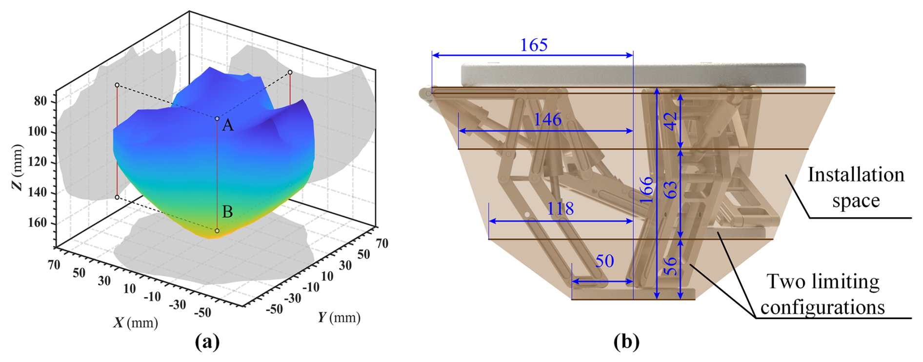
Figure 6 The workspace and the installation space of the novel 4-DOF PM: (a) the workspace, (b) the installation space.

When discussing the workspace, the singular configurations should be pointed out to avoid the phenomenon of the mechanism failing to work properly. The singular configurations are displayed in the workspace, as shown in Fig. 7. In the singular configurations, the moving platform is located on the axis z_B, and there is no rotation around the axis z_B, as represented by Eq. (33):

$$\begin{array}{}\text{(33)}& \mathit{\chi }={\left[\mathrm{0}\mathrm{0}z\mathrm{0}\right]}^{\mathrm{T}},\end{array}$$

where z is the vertical distance of the moving platform from the base.

Figure 7 The case when singularity occurs.

4.2 Stiffness analysis

The static stiffness index of the mechanism determines the kinematic accuracy and static stability of the mechanism (Tang et al., 2022). The stiffness matrix K can be calculated according to Eq. (34). The mean value of diagonal elements of the stiffness matrix is used as the stiffness performance index in this paper. The stiffness index S_tl can be expressed through Eq.(35).

$$\begin{array}{}\text{(34)}& {\displaystyle }\mathbf{K}={\mathbf{J}}^{\mathrm{T}}\mathbf{kJ}\text{(35)}& {\displaystyle }{S}_{tl}=E\left(\mathrm{tr}\right(\mathbf{K}\left)\right)\end{array}$$

In the above, J is the Jacobian matrix, and k is the stiffness matrix of the joint space.

The S_tl distribution for all workspaces is shown in Fig. 8a. S_tl tends to zero when the rotation angle around the axis z_B of the moving platform is 0° (α=0°) and the position (x, y) is close to (0, 0), as illustrated in Fig. 8b. This is the result of the singularity in this configuration. Additionally, z is negatively correlated with stiffness.

Figure 8 The stiffness distributions under (a) the whole workspace and (b) α=0°.

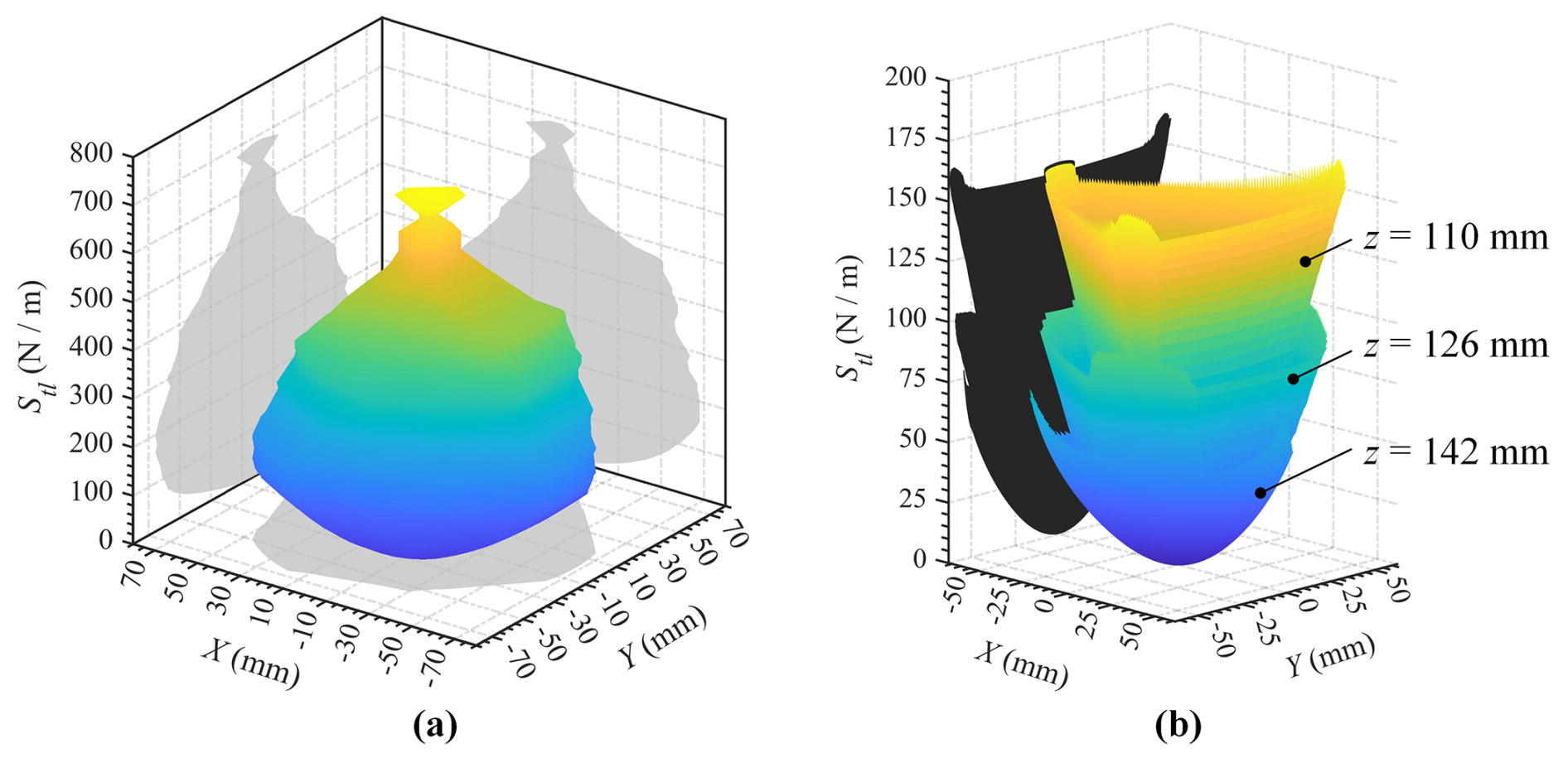
The S_tl distributions at z=110, 126, and 142 mm are shown in Fig. 9. At the same height, α is defined as 15, 30, and 45°, respectively. The results show a positive correlation between α and stiffness. However, z has less effect on the stiffness compared to α.

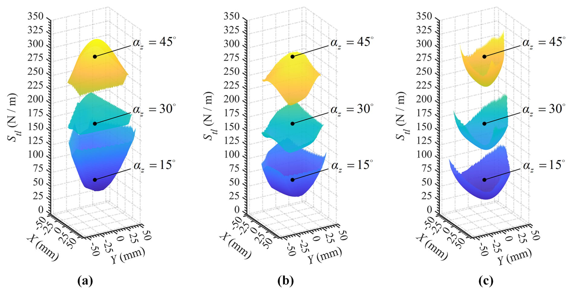
Figure 9 The stiffness distributions under the three different heights of (a) 110 mm, (b) 126 mm, and (c) 142 mm.

5 Dynamics

The Lagrange equation of the second kind is used to complete the dynamic analysis. The Lagrange equation is written in the following form:

$$\begin{array}{}\text{(36)}& {\displaystyle \frac{\mathrm{d}}{\mathrm{d}t}}\left({\displaystyle \frac{\partial L}{\partial \dot{\mathit{\chi }}}}\right)-\left({\displaystyle \frac{\partial L}{\partial \mathit{\chi }}}\right)=\mathbf{Q},\end{array}$$

where $L=K-P$ is a function called the Lagrangian, K is the kinetic energy of the system, P is the potential energy (due to gravity effects), and χ= [XYZα]^T and Q denote the vector of generalized forces applied to the system (Briot and Khalil, 2015).

The Lagrange equation can also be written in a general form of

$$\begin{array}{}\text{(37)}& \mathbf{Q}=\mathbf{M}\left(\mathit{\chi }\right)\ddot{\mathit{\chi }}+\mathbf{C}(\mathit{\chi },\dot{\mathit{\chi }})\dot{\mathit{\chi }}+\mathbf{G}\left(\mathit{\chi }\right),\end{array}$$

where M(χ) denotes the system mass matrix and is symmetric, $\mathbf{C}(\mathit{\chi },\dot{\mathit{\chi }})$ denotes the Coriolis and centrifugal matrix, and G(χ) denotes the gravity vector.

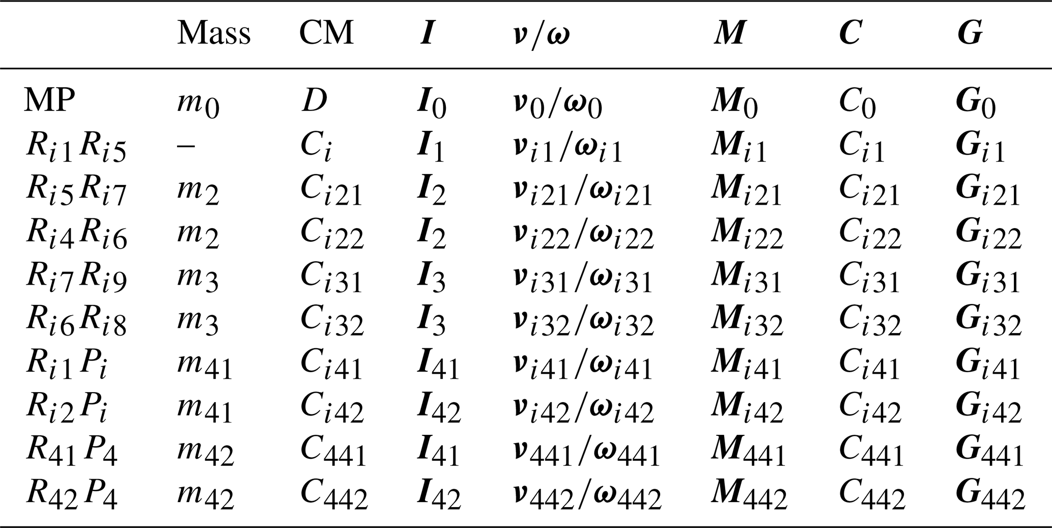
The parameters of the links are shown in Table 2. Since the link R_i6R_i7 and link R_i8R_i9 are lighter in mass, we ignore their effect on the system. MP denotes the moving platform. The link R_i1P_i and the link R_i2P_i (i=1–4) are the cylinder and piston of the actuator, respectively. CM denotes the center of mass of links, I denotes the moments of inertia of links around the center of mass, and $\mathit{v}\mathbf{/}\mathit{\omega }$ denotes the linear/angular velocity of the center of mass for links in {B}, respectively.

Table 2 The parameters of links.

5.1 Kinetic energy

The kinetic energy expression is written as follows (Taghirad, 2013):

$$\begin{array}{}\text{(38)}& K=\mathrm{1}/\mathrm{2}{\mathit{v}}^{\mathrm{T}}\mathrm{m}\mathit{v}+\mathrm{1}/\mathrm{2}{\mathit{\omega }}^{\mathrm{T}}{}^B\mathit{I}\mathit{\omega }=\mathrm{1}/\mathrm{2}{\dot{\mathit{\chi }}}^{\mathrm{T}}\mathbf{M}\left(\mathit{\chi }\right)\dot{\mathit{\chi }}.\end{array}$$

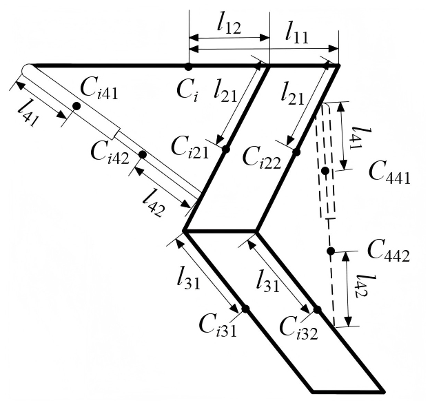
The kinetic energy of the PM is the sum of the kinetic energy of each link. The distance between the center of mass and the endpoint of each link is shown in Fig. 10.

Figure 10 Parameters of the center of mass of each link.

The coordinates of D and ^BC_i (i=1–3) of the center of mass D and C_i in {B} are known, and then the coordinate of ^BC_ijs (i=1–4; j=2–4; s=1, 2) of the center of mass C_ijs in {B} is solved as follows:

$$\begin{array}{}\text{(39)}& \left[\begin{array}{l}{}^B{\mathit{C}}_{ijs}\\ \mathrm{1}\end{array}\right]={}_{C_i}^B\mathbf{T}\left[\begin{array}{l}{}^{C_i}{\mathit{C}}_{ijs}\\ \mathrm{1}\end{array}\right]=\left[\begin{array}{l}{r}_{\mathrm{0}}c{\mathit{\theta }}_{i\mathrm{0}}+a_{i\mathrm{1}}{C}_{ijsx}\\ r_{\mathrm{0}}s{\mathit{\theta }}_{i\mathrm{0}}+a_{i\mathrm{2}}{C}_{ijsx}\\ C_{ijsz}\\ \mathrm{1}\end{array}\right],\end{array}$$

where [θ₄₀ a₄₁ a₄₂] = [θ₁₀ a₁₁ a₁₂], and ^CiC_ijs= [C_ijsx 0 C_ijsz]^T is written as

$$\begin{array}{}\text{(40)}& \begin{array}{rl}& \left[C_{ijsx}{C}_{ijsz}\right]=\left[l_{j\mathrm{3}}{c}_{j\mathrm{2}}{l}_{\mathrm{31}}\right]\left[\begin{array}{c}c{\mathit{\theta }}_{i\mathrm{2}}s{\mathit{\theta }}_{i\mathrm{2}}\\ -c{\mathit{\theta }}_{i\mathrm{3}}s{\mathit{\theta }}_{i\mathrm{3}}\end{array}\right]\\ & -\left[l_{\mathrm{1}s}\mathrm{0}\right],(i=\mathrm{1}-\mathrm{3},j=\mathrm{2},\mathrm{3}),\end{array}\end{array}$$

$$\begin{array}{}\text{(41)}& \begin{array}{rl}& \left[C_{i\mathrm{4}sx}{C}_{i\mathrm{4}sz}\right]=\left[l_{\mathrm{20}}{c}_{s\mathrm{3}}{l}_{\mathrm{4}s}{c}_{s\mathrm{4}}\right]\left[\begin{array}{ll}c{\mathit{\theta }}_{i\mathrm{2}}& s{\mathit{\theta }}_{i\mathrm{2}}\\ c{\mathit{\theta }}_{i\mathrm{4}}& -s{\mathit{\theta }}_{i\mathrm{4}}\end{array}\right]\\ & -\left[l_{\mathrm{1}s}{c}_{s\mathrm{4}}\mathrm{0}\right],(i=\mathrm{1}-\mathrm{3}),\end{array}\end{array}$$

$$\begin{array}{}\text{(42)}& \begin{array}{rl}\left[C_{\mathrm{44}sx}{C}_{\mathrm{44}sz}\right]=\left[l_{s\mathrm{4}}-l_{\mathrm{4}s}{c}_{s\mathrm{4}}\right]& \left[\begin{array}{ll}c{\mathit{\theta }}_{\mathrm{12}}s{\mathit{\theta }}_{\mathrm{12}}& \\ c({\mathit{\theta }}_{\mathrm{12}}+{\mathit{\theta }}_{\mathrm{44}})& s({\mathit{\theta }}_{\mathrm{12}}+{\mathit{\theta }}_{\mathrm{44}})\end{array}\right]\\ +l_{\mathrm{30}}{c}_{s\mathrm{3}}\left[\begin{array}{l}-c{\mathit{\theta }}_{\mathrm{13}}\\ s{\mathit{\theta }}_{\mathrm{13}}\end{array}\right]-\left[l_{\mathrm{11}}\mathrm{0}\right],\end{array}\end{array}$$

where $c_{\mathrm{22}}=c_{\mathrm{13}}=\mathrm{0}$, $c_{\mathrm{32}}=c_{\mathrm{23}}=c_{\mathrm{24}}=\mathrm{1}$, $c_{\mathrm{14}}=-\mathrm{1}$, l₂₃=l₂₁, $l_{\mathrm{33}}=l_{\mathrm{24}}=l_{\mathrm{2}}$, and $l_{\mathrm{14}}=l_{\mathrm{2}}-l_{\mathrm{20}}$; θ_i4 (i=1–4) is given using the cosine theorem for triangle R_i1R_i2R_i4 (i=1–3) and triangle R₄₁R₄₂R₁₇ again.

$$\begin{array}{}\text{(43)}& {\mathit{\theta }}_{i\mathrm{4}}=\arccos \mathrm{2}\left(c_{i\mathrm{5}}+L_i^{\mathrm{2}},\mathrm{2}{c}_{i\mathrm{6}}{L}_i\right)\end{array}$$

In the above, $c_{i\mathrm{5}}=(l_{\mathrm{1}}-l_{\mathrm{10}}{)}^{\mathrm{2}}$ – $l_{\mathrm{20}}^{\mathrm{2}}$, c_i6=l₁ – l₁₀ (i=1–3), $c_{\mathrm{45}}=l_{\mathrm{20}}^{\mathrm{2}}$ – $l_{\mathrm{30}}^{\mathrm{2}}$, and c₄₆=l₂₀.

θ_i1 (i=1–3) is used to solve the linear and angular velocities of the center of mass of links, and then it is given from the equivalence of Eqs. (7) and (8) as follows:

$$\begin{array}{}\text{(44)}& {\mathit{\theta }}_{i\mathrm{1}}=\arctan \mathrm{2}\left(a_{i\mathrm{25}},a_{i\mathrm{15}}\right),\end{array}$$

where [a_i15a_i25] (i=1–3) is written as

$$\begin{array}{}\text{(45)}& \left[a_{i\mathrm{15}}{a}_{i\mathrm{25}}\right]=\left[XY{c}_{i\mathrm{7}}\right]\left[\begin{array}{cc}\mathrm{1}& -\sqrt{\mathrm{3}}{c}_i\\ \sqrt{\mathrm{3}}{c}_i& \mathrm{1}\\ r\mathrm{c}\mathit{\alpha }-r_{\mathrm{0}}& r\mathrm{s}\mathit{\alpha }\end{array}\right],\end{array}$$

where c₁₇=1, and $c_{\mathrm{27}}=c_{\mathrm{37}}=-\mathrm{2}$.

The center-of-mass linear and angular velocities of links in {B} are obtained by differentiating χ= [D α]^T, ^BC_i (i=1–3), and ^BC_ijs (i=1–4; j=2–4; s=1, 2) with respect to time as follows:

$$\begin{array}{}\text{(46)}& \left[\begin{array}{cc}{\mathit{v}}_{\mathrm{0}}& {\mathit{\omega }}_{\mathrm{0}}\\ {\mathit{v}}_{i\mathrm{1}}& {\mathit{\omega }}_{i\mathrm{1}}\\ {\mathit{v}}_{ijs}& {\mathit{\omega }}_{ijs}\end{array}\right]=\left[\begin{array}{cc}{\mathbf{B}}_{\mathrm{01}}& {\mathbf{B}}_{\mathrm{02}}\\ {\mathbf{0}}_{\mathrm{3}\times \mathrm{4}}& {\mathbf{B}}_{i\mathrm{12}}\\ {\mathbf{B}}_{ijs\mathrm{1}}& {\mathbf{B}}_{ijs\mathrm{2}}\end{array}\right]\dot{\mathit{\chi }},\end{array}$$

where B₀₁, B₀₂, B_i12 (i = 1–3), B_ijs1, and B_ijs2 (i = 1–4; j = 2–4; s = 1, 2) are all 3 × 4 matrixes and are written as

$$\begin{array}{}\text{(47)}& \left\{\begin{array}{cc}& {\mathbf{B}}_{\mathrm{01}}=\left[{\mathit{I}}_{\mathrm{3}\times \mathrm{3}}{\mathbf{0}}_{\mathrm{3}\times \mathrm{1}}\right],{\mathbf{B}}_{\mathrm{02}}=\left[\begin{array}{ll}{\mathbf{0}}_{\mathrm{3}\times \mathrm{3}}& \mathrm{0}\\ & \mathrm{0}\\ & \mathrm{1}\end{array}\right],\\ & {\mathbf{B}}_{i\mathrm{12}}=\left[\begin{array}{c}{\mathbf{0}}_{\mathrm{2}\times \mathrm{4}}\\ {\mathit{b}}_{i\mathrm{1}}\end{array}\right]\\ & {\mathbf{B}}_{ijs\mathrm{1}}=\left[\begin{array}{c}{C}_{ijsx}{\mathit{b}}_{i\mathrm{10}}+a_{i\mathrm{1}}{\mathit{b}}_{ijsx}\\ C_{ijsz}{\mathit{b}}_{i\mathrm{20}}+a_{i\mathrm{2}}{\mathit{b}}_{ijsx}\\ {\mathit{b}}_{ijsz}\end{array}\right],\\ & {\mathbf{B}}_{ijs\mathrm{2}}={}_{C_i}^B\mathit{R}\left[\begin{array}{l}{\mathbf{0}}_{\mathrm{1}\times \mathrm{4}}\\ {\mathit{b}}_{\underset{\mathrm{¯}}{ij}}\\ {\mathit{b}}_{i\mathrm{1}}\end{array}\right],\end{array}\right.\end{array}$$

where b_i1 (i=1–3), ${\mathit{b}}_{\underset{\mathrm{¯}}{ij}}$, b_i10, b_i20, b_ijsx and b_ijsz (i=1–4; j=2–4; s=1, 2) are all 1 × 4 matrixes and are solved by differentiating θ_i1, θ_i4, C_ijsx, and C_ijsz with respect to time (${\mathit{\theta }}_{\underset{\mathrm{¯}}{\mathrm{44}}}={\mathit{\theta }}_{\mathrm{44}}$ +θ₁₂, ${\mathit{b}}_{\underset{\mathrm{¯}}{ij}}=$ b_ij, and ${\mathit{b}}_{\underset{\mathrm{¯}}{\mathrm{44}}}=$ b₄₄+ b₁₂; b_i4 is unknown).

$$\begin{array}{}\text{(48)}& \left[{\dot{\mathit{\theta }}}_{i\mathrm{1}}{\dot{\mathit{\theta }}}_{i\mathrm{4}}\right]=\left[{\mathit{b}}_{i\mathrm{1}}{\mathit{b}}_{i\mathrm{4}}\right]\dot{\mathit{\chi }}\end{array}$$

$$\begin{array}{}\text{(49)}& {\mathit{b}}_{i\mathrm{1}}=\left[a_{i\mathrm{15}}{a}_{i\mathrm{25}}\right]{\displaystyle \frac{{\mathbf{B}}_{i\mathrm{2}}}{a_{i\mathrm{8}}}},{\mathit{b}}_{i\mathrm{4}}=-{\displaystyle \frac{(L_i^{\mathrm{2}}-c_{i\mathrm{5}})a_{i\mathrm{6}}{\mathit{b}}_{i\mathrm{2}}}{\mathrm{2}{c}_{i\mathrm{6}}{L}_i^{\mathrm{2}}{a}_{i\mathrm{9}}}}\end{array}$$

$$\begin{array}{}\text{(50)}& \left\{\begin{array}{c}{\mathbf{B}}_{i\mathrm{2}}=\left[\begin{array}{cccc}r{c}_{i\mathrm{5}}\mathrm{c}\mathit{\alpha }& a_{i\mathrm{15}}& \mathrm{0}& -\sqrt{\mathrm{3}}{c}_i\\ r{c}_{i\mathrm{5}}\mathrm{s}\mathit{\alpha }& a_{i\mathrm{25}}& \mathrm{0}& -\mathrm{1}\end{array}\right]\\ a_{i\mathrm{8}}=\left[\begin{array}{cc}{a}_{i\mathrm{15}}& a_{i\mathrm{25}}\end{array}\right]{\left[\begin{array}{cc}\mathrm{1}& -\sqrt{\mathrm{3}}{c}_i\end{array}\right]}^{\mathrm{T}}\\ a_{i\mathrm{9}}=\sqrt{\mathrm{1}-{\left(\frac{c_{i\mathrm{5}}+L_i^{\mathrm{2}}}{\mathrm{2}{c}_{i\mathrm{6}}{L}_i}\right)}^{\mathrm{2}}}\end{array}\right.\end{array}$$

$$\begin{array}{}\text{(51)}& {\mathit{b}}_{i\mathrm{10}}=-a_{i\mathrm{2}}{\mathit{b}}_{i\mathrm{1}},{\mathit{b}}_{i\mathrm{20}}=a_{i\mathrm{1}}{\mathit{b}}_{i\mathrm{1}},\left({\mathit{b}}_{\mathrm{410}}={\mathit{b}}_{\mathrm{110}},{\mathit{b}}_{\mathrm{420}}={\mathit{b}}_{\mathrm{120}}\right)\end{array}$$

$$\begin{array}{}\text{(52)}& \left\{\begin{array}{c}\left[{\mathit{b}}_{ijsx}{\mathit{b}}_{ijsz}\right]=\left[l_{j\mathrm{3}}{c}_{j\mathrm{2}}{l}_{\mathrm{31}}\right]\left[\begin{array}{ll}-s{\mathit{\theta }}_{i\mathrm{2}}{\mathit{b}}_{i\mathrm{2}}& c{\mathit{\theta }}_{i\mathrm{2}}{\mathit{b}}_{i\mathrm{2}}\\ s{\mathit{\theta }}_{i\mathrm{3}}{\mathit{b}}_{i\mathrm{3}}& c{\mathit{\theta }}_{i\mathrm{3}}{\mathit{b}}_{i\mathrm{3}}\end{array}\right]\\ \left[{\mathit{b}}_{i\mathrm{4}sx}{\mathit{b}}_{i\mathrm{4}sz}\right]=\left[l_{\mathrm{20}}{c}_{s\mathrm{3}}{l}_{\mathrm{4}s}{c}_{s\mathrm{4}}\right]\left[\begin{array}{ll}-s{\mathit{\theta }}_{i\mathrm{2}}{\mathit{b}}_{i\mathrm{2}}& c{\mathit{\theta }}_{i\mathrm{2}}{\mathit{b}}_{i\mathrm{2}}\\ -s{\mathit{\theta }}_{i\mathrm{4}}{\mathit{b}}_{i\mathrm{4}}& -c{\mathit{\theta }}_{i\mathrm{4}}{\mathit{b}}_{i\mathrm{4}}\end{array}\right]\\ \left[{\mathit{b}}_{\mathrm{44}sx}{\mathit{b}}_{\mathrm{44}sz}\right]=-\left[l_{s\mathrm{4}}{l}_{\mathrm{4}s}{c}_{s\mathrm{4}}\right]\left[\begin{array}{ll}s{\mathit{\theta }}_{\mathrm{12}}{\mathit{b}}_{\mathrm{12}}& c{\mathit{\theta }}_{\mathrm{12}}{\mathit{b}}_{\mathrm{12}}\\ s{\mathit{\theta }}_{\underset{\mathrm{¯}}{\mathrm{44}}}{\mathit{b}}_{\underset{\mathrm{¯}}{\mathrm{44}}}& c{\mathit{\theta }}_{\underset{\mathrm{¯}}{\mathrm{44}}}{\mathit{b}}_{\underset{\mathrm{¯}}{\mathrm{44}}}\end{array}\right]\\ +l_{\mathrm{30}}{c}_{s\mathrm{3}}\left[\mathrm{s}{\mathit{\theta }}_{\mathrm{13}}{\mathit{b}}_{\mathrm{13}}\mathrm{c}{\mathit{\theta }}_{\mathrm{13}}{\mathit{b}}_{\mathrm{13}}\right]\end{array}\right.\end{array}$$

The rotation matrix around the y axis and moments of inertia are expressed as follows:

$$\begin{array}{}\text{(53)}& \begin{array}{r}{\mathbf{R}}_y{(}^{\ast })=\left[\begin{array}{ccc}{\mathrm{c}}^{\ast }& \mathrm{0}& {\mathrm{s}}^{\ast }\\ \mathrm{0}& \mathrm{1}& \mathrm{0}\\ -{\mathrm{s}}^{\ast }& \mathrm{0}& {\mathrm{c}}^{\ast }\end{array}\right]\\ I=\left[\begin{array}{lll}{\mathbf{I}}_{xx}& \mathrm{0}& \mathrm{0}\\ \mathrm{0}& {\mathit{I}}_{yy}& \mathrm{0}\\ \mathrm{0}& \mathrm{0}& {\mathit{I}}_{zz}\end{array}\right].\end{array}\end{array}$$

The moments of inertia ^BI₀, ^BI_i1 (i=1–3), and ^BI_ijs (i=1–4; j=2–4; s=1, 2) are written as follows:

$$\begin{array}{}\text{(54)}& \left[\begin{array}{c}{}^B{I}_{\mathrm{0}}\\ {}^B{\mathit{I}}_{i\mathrm{1}}\\ {}^B{\mathit{I}}_{ijs}\end{array}\right]=\left[\begin{array}{c}{}_D^B\mathit{R}{\mathit{I}}_{\mathrm{0}}{}_D^B{\mathit{R}}^{\mathrm{T}}\\ {}_{C_i}^B\mathit{R}{\mathit{I}}_{\mathrm{1}}{}_{C_i}^B{\mathit{R}}^{\mathrm{T}}\\ {}_{C_i}^B\mathit{R}{\mathit{R}}_y\left({\mathit{\theta }}_{ijs}\right){\mathit{I}}_{js}{\left({}_{C_i}^B\mathit{R}{\mathit{R}}_y\left({\mathit{\theta }}_{ijs}\right)\right)}^{\mathrm{T}}\end{array}\right],\end{array}$$

where I_js= I_j (j=2, 3), ${\mathit{\theta }}_{ijs}=\mathit{\pi }/\mathrm{2}-{\mathit{\theta }}_{ij}$, and ${\mathit{\theta }}_{\mathrm{44}s}={\mathit{\theta }}_{\underset{\mathrm{¯}}{\mathrm{44}}}-\mathit{\pi }/\mathrm{2}$.

Substituting Eqs. (46) and (54) into Eq. (38) yields the mass matrix M₀ (χ), M_i1 (χ) (i=1–3), and M_ijs (χ) (i=1–4; j=2–4; s=1, 2) as follows:

$$\begin{array}{}\text{(55)}& {\mathbf{M}}_{\mathrm{0}}\left(\mathit{\chi }\right)=\left[\begin{array}{cc}{m}_{\mathrm{0}}{\mathit{I}}_{\mathrm{3}\times \mathrm{3}}& {\mathbf{0}}_{\mathrm{3}\times \mathrm{1}}\\ {\mathbf{0}}_{\mathrm{1}\times \mathrm{3}}& {\mathit{I}}_{\mathrm{0}\mathrm{ZZ}}\end{array}\right],\end{array}$$

$$\begin{array}{}\text{(56)}& \left[\begin{array}{c}{\mathbf{M}}_{i\mathrm{1}}\left(\mathit{\chi }\right)\\ {\mathbf{M}}_{ijs}\left(\mathit{\chi }\right)\end{array}\right]=\left[\begin{array}{c}{\mathbf{B}}_{i\mathrm{12}}^{\mathrm{T}}{}^B{\mathbf{I}}_{i\mathrm{1}}{\mathbf{B}}_{i\mathrm{12}}\\ {\mathbf{B}}_{ijs\mathrm{1}}^{\mathrm{T}}{m}_{ijs}{\mathbf{B}}_{ijs\mathrm{1}}+{\mathbf{B}}_{ijs\mathrm{2}}^{\mathrm{T}}{}^B{\mathbf{I}}_{ijs}{\mathbf{B}}_{ijs\mathrm{2}}\end{array}\right].\end{array}$$

5.2 Potential energy

The potential energy P is written as follows:

$$\begin{array}{}\text{(57)}& P=-m\mathit{g}{z}_C,\end{array}$$

where z_C is the coordinate of the center of mass of the link in the z_B axis.

The total potential energy of the mechanism is the sum of the potential energy of each link. The relationship between the gravity vector of each link and the potential energy is

$$\begin{array}{}\text{(58)}& \mathbf{G}\left(\mathit{\chi }\right)={\displaystyle \frac{\partial P}{\partial \mathit{\chi }}}.\end{array}$$

According to Eq. (58), the gravity vectors of G₀(χ), G_i1(χ) (i=1–3), and G_ijs(χ) (i=1–4; j=2–4; s=1, 2) are written as follows:

$$\begin{array}{}\text{(59)}& \left[{\mathit{G}}_{\mathrm{0}}\left(\mathit{\chi }\right){\mathit{G}}_{i\mathrm{1}}\left(\mathit{\chi }\right){\mathit{G}}_{ijs}\left(\mathit{\chi }\right)\right]=\left[{\left[\mathrm{0}\mathrm{0}-m_{\mathrm{0}}g\mathrm{0}\right]}^{\mathrm{T}}{\mathbf{0}}_{\mathrm{4}\times \mathrm{1}}-m_{ijs}g{\mathit{b}}_{ijsz}^{\mathrm{T}}\right].\end{array}$$

5.3 Dynamic equations

The generalized force can be obtained as follows:

$$\begin{array}{}\text{(60)}& \mathbf{Q}=\mathbf{M}\left(\mathit{\chi }\right)\ddot{\mathit{\chi }}+\mathbf{C}(\mathit{\chi },\dot{\mathit{\chi }})\dot{\mathit{\chi }}+\mathbf{G}\left(\mathit{\chi }\right).\end{array}$$

According to the principle of virtual work, the relationship among the force of the actuated joint τ, the vector of the generalized force Q, and the external load f acting on the moving platform can be expressed as follows:

$$\begin{array}{}\text{(61)}& \mathbf{Q}+\mathbf{f}={\mathbf{J}}^{\mathrm{T}}\mathit{\tau }.\end{array}$$

Thus, the general equation of the actuator force is obtained as

$$\begin{array}{}\text{(62)}& \mathit{\tau }={\mathbf{J}}^{-\mathrm{T}}\left(\mathbf{M}\left(\mathit{\chi }\right)\ddot{\mathit{\chi }}+\mathbf{C}(\mathit{\chi },\dot{\mathit{\chi }})\dot{\mathit{\chi }}+\mathbf{G}\left(\mathit{\chi }\right)+\mathbf{f}\right),\end{array}$$

where M(χ) and $\mathbf{C}(\mathit{\chi },\dot{\mathit{\chi }})$ are 4 × 4 matrixes, and G(χ) is a 4 × 1 matrix.

$$\begin{array}{}\text{(63)}& \left\{\begin{array}{l}\mathit{M}\left(\mathit{\chi }\right)={\mathit{M}}_{\mathrm{0}}\left(\mathit{\chi }\right)+\sum _{i=\mathrm{1}}^{\mathrm{3}}{\mathit{M}}_{i\mathrm{1}}\left(\mathit{\chi }\right)+\sum _{i=\mathrm{1}}^{\mathrm{4}}\sum _{j=\mathrm{2}}^{\mathrm{4}}\sum _{s=\mathrm{1}}^{\mathrm{2}}{\mathit{M}}_{ijs}\left(\mathit{\chi }\right)\\ \mathit{G}\left(\mathit{\chi }\right)={\mathit{G}}_{\mathrm{0}}\left(\mathit{\chi }\right)+\sum _{i=\mathrm{1}}^{\mathrm{3}}{\mathit{G}}_{i\mathrm{1}}\left(\mathit{\chi }\right)+\sum _{i=\mathrm{1}}^{\mathrm{4}}\sum _{j=\mathrm{2}}^{\mathrm{4}}\sum _{s=\mathrm{1}}^{\mathrm{2}}{\mathit{G}}_{ijs}\left(\mathit{\chi }\right)\\ \mathit{C}(\mathit{\chi },\dot{\mathit{\chi }})={\mathit{C}}_{\mathrm{0}}(\mathit{\chi },\dot{\mathit{\chi }})+\sum _{i=\mathrm{1}}^{\mathrm{3}}{\mathit{C}}_{i\mathrm{1}}(\mathit{\chi },\dot{\mathit{\chi }})+\sum _{i=\mathrm{1}}^{\mathrm{4}}\sum _{j=\mathrm{2}}^{\mathrm{4}}\sum _{s=\mathrm{1}}^{\mathrm{2}}\\ {\mathit{C}}_{ijs}(\mathit{\chi },\dot{\mathit{\chi }})\end{array}\right.\end{array}$$

The Coriolis and centrifugal matrix is expressed as follows:

$$\begin{array}{}\text{(64)}& \begin{array}{rl}& \mathbf{C}(\mathit{\chi },\dot{\mathit{\chi }})=\mathrm{1}/\mathrm{2}\left(\dot{\mathbf{M}}\left(\mathit{\chi }\right)+{\mathbf{U}}^{\mathrm{T}}-\mathbf{U}\right),\\ & \mathbf{U}=\left({\mathbf{I}}_{\mathrm{4}\times \mathrm{4}}\otimes {\dot{\mathit{\chi }}}^{\mathrm{T}}\right){\displaystyle \frac{\partial \mathbf{M}\left(\mathit{\chi }\right)}{\partial \mathit{\chi }}}.\end{array}\end{array}$$

The terms in the matrix M₀(χ) are constants, and so it could be obtained that

$$\begin{array}{}\text{(65)}& \begin{array}{rl}{\dot{\mathbf{M}}}_{\mathrm{0}}\left(\mathit{\chi }\right)& =\mathbf{0},{\displaystyle \frac{\partial {\mathbf{M}}_{\mathrm{0}}\left(\mathit{\chi }\right)}{\partial \mathit{\chi }}}=\mathbf{0},{\mathbf{C}}_{\mathrm{0}}(\mathit{\chi },\dot{\mathit{\chi }})\\ & =\mathrm{1}/\mathrm{2}\left({\dot{\mathbf{M}}}_{\mathrm{0}}\right(\mathit{\chi })+{\mathbf{U}}_{\mathrm{0}}^{\mathrm{T}}-{\mathbf{U}}_{\mathrm{0}})=\mathbf{0}.\end{array}\end{array}$$

The solution procedures for C_i1(χ) and ${\mathbf{C}}_{ijs}(\mathit{\chi },\dot{\mathit{\chi }})$ are shown in Appendix B.

6 Simulation verification

All links are fabricated from standard carbon steel with a density of $\mathrm{7.801}\times {\mathrm{10}}^{-\mathrm{6}}$ kg mm⁻³, and the parameters of the PM are listed in Table 3.

Table 3 The parameter values of the PM.

θ₁₀=0, ${\mathit{\theta }}_{\mathrm{20}}=\mathrm{2}/\mathrm{3}\mathit{\pi }$, and ${\mathit{\theta }}_{\mathrm{30}}=-\mathrm{2}/\mathrm{3}\mathit{\pi }$. The initial position and orientation vector of point D in the base frame {B} was defined as χ= [−5.5491 12.7839 110 −0.2654]^T so that singularity can be avoided, and $\ddot{\mathit{\chi }}=$ [8t 8t 8t 0.07t]^T. Gravitational acceleration (g = 9.8 N kg⁻¹) was enabled in the simulation model, and an external load f = [f₁ f₂f₃f₄]^T= [25 25 50 25]^T was applied to the center of the moving platform. Herein, f₁, f₂, and f₃, represent the translational force (N) along the X, Y, and Z axes, respectively, and f₄ denotes the rotational moment (N m) about the Z axis.

Based on the aforementioned parameters and physical quantities, the theoretical results and Adams simulation results of the actuator displacement (L), velocity (V), acceleration (A), and driving force (F) are obtained separately, and excellent agreement was observed between the two sets of results. The simulation curves derived from Adams are presented in Fig. 11a–d.

To quantitatively describe the similarity between the simulation results and the theoretical results of the driving rod, the error existing between them was calculated. The error was calculated using the following formula:

$$\begin{array}{}\text{(66)}& {\mathrm{\Delta }}_h=h_T-h_S,\left(h=L,V,A,F\right),\end{array}$$

where h_T and h_S denote the theoretical and simulation results of the L, V, A, and F, respectively, and Δ_h is the error value between h_T and h_S.

The time-varying curves of the error Δ_h are obtained according to Eq. (66), as shown in Fig. 12a–d.

In general, the magnitude of the error Δ_h is dependent on the magnitude of the simulated value, with larger actual values leading to greater absolute errors. Thus, the error ratio σ_h for the L, V, A, and F is defined. It can be defined as follows:

$$\begin{array}{}\text{(67)}& {\mathit{\sigma }}_h=\left|{\mathrm{\Delta }}_{h\max }\right|/h_S,\left(h=L,V,A,F\right),\end{array}$$

where Δ_hmax is the maximum absolute error, and h_S is the corresponding simulation result at the same time instant.

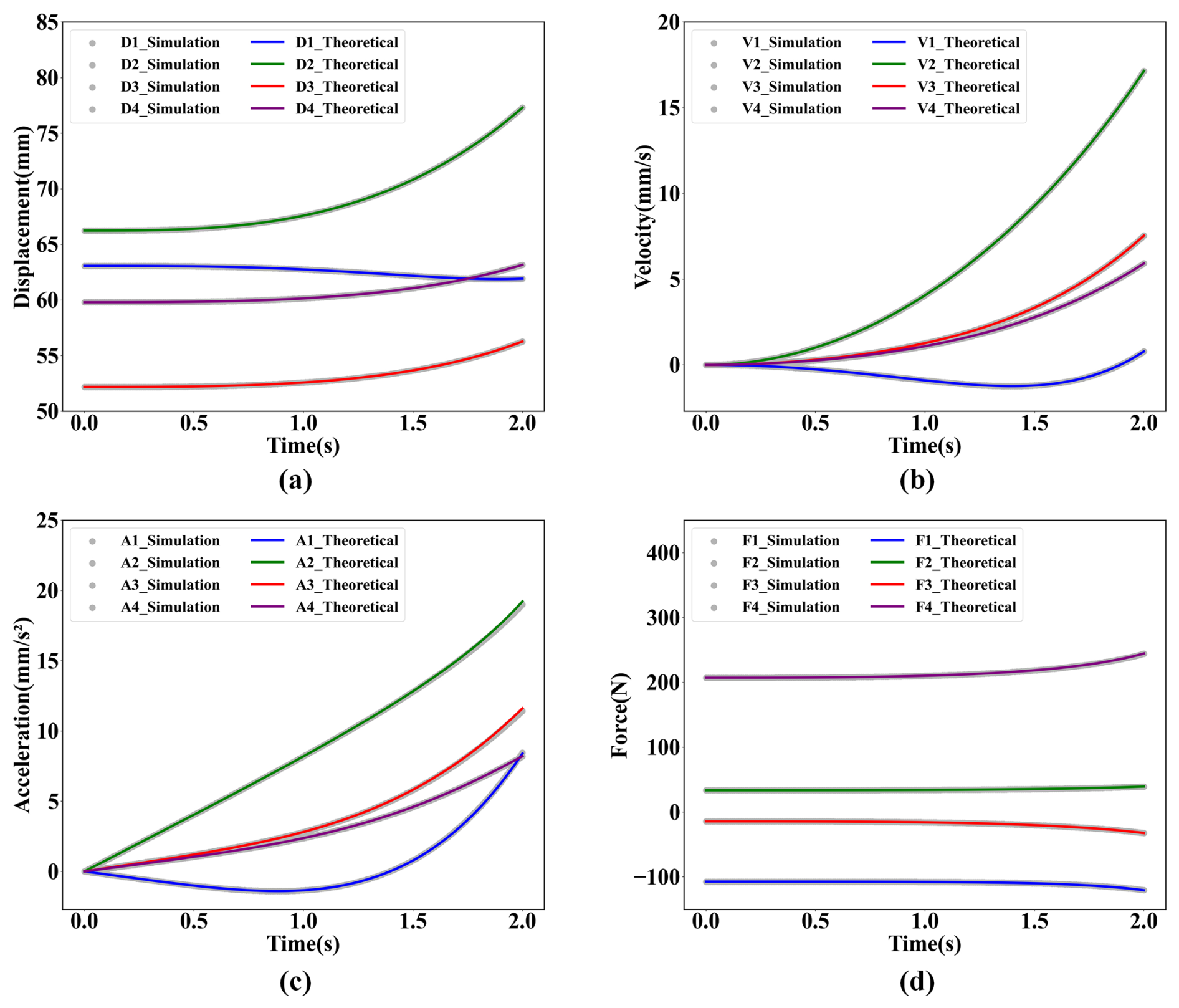
Figure 11 Actuator simulation curves: (a) displacement, (b) velocity, (c) acceleration, and (d) force.

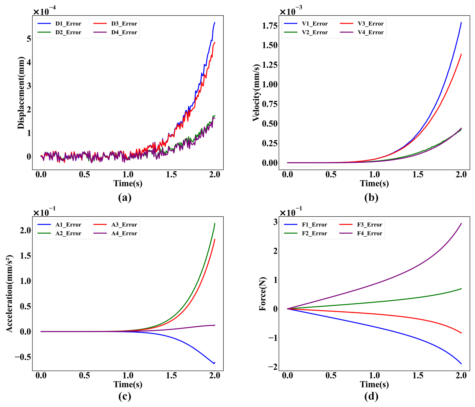
Figure 12 The error value curves between theoretical results and simulation results: (a) displacement, (b) velocity, (c) acceleration, and (d) force.

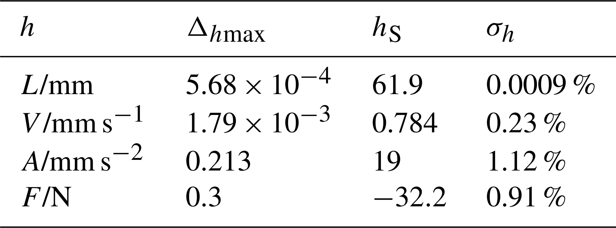
The error ratios σ_h were calculated based on Figs. 11 and 12, as listed in Table 4. It can be seen that the error ratios of the actuator displacement, velocity, acceleration, and driving force were 0.0009 %, 0.23 %, 1.12 %, and 0.91 %, respectively. The extremely small error ratios confirm the correctness of the established kinematic and dynamic models of the PM.

Table 4 The error parameters between theoretical results and simulation results.

7 Conclusions

A novel 4-DOF PM with the 3-RPaPaR limb is proposed in this paper; this PM is capable of implementing three-translation and one-rotation (3T1R) motion and features a large workspace. Most kinematic joints of the mechanism are revolute joints, forming a sub-closed-loop parallelogram structure that endows the mechanism with promising application prospects in high-speed and heavy-load fields. The degree-of-freedom characteristics of the mechanism are verified using screw theory, and inverse position, velocity, and acceleration models of the mechanism are established systematically. The singular configurations of the mechanism are found to be distributed on z_B without offset. The rotation angle α of the moving platform is identified as the dominant factor affecting the stiffness performance of the mechanism, while the vertical height z has a secondary effect. An explicit inverse dynamic model is derived based on the Lagrange equations of the second kind. The correctness of the established kinematic and dynamic theoretical models is verified by Adams simulations, with the error ratios of key actuator performance indices all remaining at an extremely low level. The modeling method presented in this paper can serve as a reference for kinematic and dynamic modeling of other PMs with four-joint sub-closed-loop limbs, and it is expected to promote the engineering application of this type of PM in industrial practice.

Appendix A

This section supplements the solution procedure for ${\dot{\mathit{b}}}_{i\mathrm{2}}$ (i=1–4) in Eq. (31). Since ${\dot{\mathit{b}}}_{\mathrm{42}}={\dot{\mathit{b}}}_{\mathrm{12}}+{\dot{\mathit{b}}}_{\mathrm{13}}$, the solution of ${\dot{\mathit{b}}}_{i\mathrm{2}}$ can be converted into solving ${\dot{\mathit{b}}}_{ij}$ (i=1–3; j=2, 3).

To simplify subsequent calculations, ${\dot{\mathit{b}}}_{ij}$ and ∂b${}_{ij}/\partial$ χ are combined into b${}_{ij}^{\prime }$, and this operation is extended to other equations. An operator I* and c are defined for derivation. For time differentiation, I* =1, $c^{\prime }=\mathrm{0}$, and ${\mathit{\chi }}^{\prime }=\dot{\mathit{\chi }}$; for partial differentiation with respect to χ, I* represents the Kronecker product (⊗) of the identity matrix I_4×4 and the corresponding matrix, $c^{\prime }=$0_4×1, and ${\mathit{\chi }}^{\prime }=$ [$X^{\prime }{Y}^{\prime }{Z}^{\prime }{\mathit{\alpha }}^{\prime }$]^T. In addition, $\mathit{\chi }(i{)}^{\prime }=$ I_4×4(i)^T, (i) denotes the ith row of the matrix.

b${}_{ij}^{\prime }=$ [$a_{ij\mathrm{1}}^{\prime }{a}_{ij\mathrm{2}}^{\prime }$ $a_{ij\mathrm{3}}^{\prime }{a}_{ij\mathrm{4}}^{\prime }$] (i=1–3; j=2, 3) is obtained by time differentiation of Eq. (23), as shown below:

$$\begin{array}{}\text{(A1)}& \begin{array}{rl}& {\left[\begin{array}{l}{a}_{ij\mathrm{1}}^{\prime }\\ a_{ij\mathrm{2}}^{\prime }\\ a_{ij\mathrm{4}}^{\prime }\end{array}\right]}^{\mathrm{T}}={\mathit{b}}_{ij\mathrm{1}}^{\prime }{\mathbf{B}}_{i\mathrm{1}}+\mathit{I}\ast {\mathit{b}}_{ij\mathrm{1}}\\ & \left[\begin{array}{lll}\mathrm{2}{X}^{\prime }& \mathrm{2}{Y}^{\prime }& \mathrm{2}{r}_{\mathrm{0}}r\mathrm{c}\mathit{\alpha }{\mathit{\alpha }}^{\prime }\\ {\mathrm{0}}^{\prime }& {\mathrm{0}}^{\prime }& \sqrt{\mathrm{3}}{c}_i{X}^{\prime }-Y^{\prime }\\ {\mathrm{0}}^{\prime }& {\mathrm{0}}^{\prime }& X^{\prime }+\sqrt{\mathrm{3}}{c}_i{Y}^{\prime }\end{array}\right],\\ & a_{ij\mathrm{3}}^{\prime }={\mathit{b}}_{ij\mathrm{2}}^{\prime }{\mathit{b}}_{ij\mathrm{3}}+\mathit{I}\ast {\mathit{b}}_{ij\mathrm{2}}{\mathit{b}}_{ij\mathrm{3}}^{\prime },\end{array}\end{array}$$

where b${}_{ij\mathrm{1}}^{\prime }$, b${}_{ij\mathrm{2}}^{\prime }$, and b${}_{ij\mathrm{3}}^{\prime }$ are given by

$$\begin{array}{}\text{(A2)}& {\displaystyle }\begin{array}{rl}& {\mathit{b}}_{ij\mathrm{1}}^{\prime }=\left(\left(({\mathit{b}}_{ij\mathrm{2}}^{\prime }{\mathit{b}}_{ij\mathrm{4}}+\mathit{I}\ast {\mathit{b}}_{ij\mathrm{2}}{\mathit{b}}_{ij\mathrm{4}}^{\prime }){\mathit{b}}_{ij\mathrm{5}}+{\mathit{b}}_{ij\mathrm{2}}{\mathit{b}}_{ij\mathrm{4}}{\mathit{b}}_{ij\mathrm{5}}^{\prime }\right)\right.\\ & \left.a_{i\mathrm{7}}-\mathrm{2}{a}_{i\mathrm{4}}^{\prime }{\mathit{b}}_{ij\mathrm{2}}{\mathit{b}}_{ij\mathrm{4}}{\mathit{b}}_{ij\mathrm{5}}\right)/a_{i\mathrm{7}}^{\mathrm{2}},\end{array}\text{(A3)}& {\displaystyle }\begin{array}{rl}& {\mathit{b}}_{ij\mathrm{2}}^{\prime }={\displaystyle \frac{-a_{i\mathrm{3}}^{\prime }}{a_{i\mathrm{3}}}}{\left(\left[{\displaystyle \frac{a_{ij\mathrm{5}}-(a_{i\mathrm{3}}+(l_{\mathrm{2}}^{\mathrm{2}}-l_{\mathrm{3}}^{\mathrm{2}}\left)c_j\right)a_{ij\mathrm{6}}}{a_{ij\mathrm{5}}^{\mathrm{2}}}}\mathrm{0}\right]-{\mathit{b}}_{ij\mathrm{2}}\right)}^{\prime },\\ & {\mathit{b}}_{ij\mathrm{3}}=\left[\begin{array}{l}{Z}^{\prime }\\ a_{i\mathrm{4}}^{\prime }\end{array}\right].\end{array}\end{array}$$

Time differentiation of Eq. (25) yields b${}_{ij\mathrm{4}}^{\prime }$, b${}_{ij\mathrm{5}}^{\prime }$, and $a_{ij\mathrm{6}}=a_{ij\mathrm{5}}^{\prime }/a_{i\mathrm{3}}^{\prime }$ (i=1–3) as follows:

$$\begin{array}{}\text{(A4)}& \begin{array}{rl}& {\mathit{b}}_{ij\mathrm{4}}^{\prime }=\left[\begin{array}{l}{a}_{i\mathrm{4}}^{\prime }\\ -Z^{\prime }\end{array}\right],{\mathit{b}}_{ij\mathrm{5}}^{\prime }=r{c}_{i\mathrm{0}}\left[{\mathbf{0}}_{\mathrm{4}\times \mathrm{1}}-\mathrm{s}\mathit{\alpha }{\mathit{\alpha }}^{\prime }\mathrm{c}\mathit{\alpha }{\mathit{\alpha }}^{\prime }\right],\\ & a_{ij\mathrm{6}}=\left(\mathrm{2}{l}_j^{\mathrm{2}}+(l_{\mathrm{2}}^{\mathrm{2}}-l_{\mathrm{3}}^{\mathrm{2}}-c_j{a}_{i\mathrm{3}})c_j\right)/a_{ij\mathrm{5}}.\end{array}\end{array}$$

Time differentiation of Eq. (16) gives $a_{i\mathrm{3}}^{\prime }$ and $a_{i\mathrm{4}}^{\prime }$ (i=1–3).

$$\begin{array}{}\text{(A5)}& \left\{\begin{array}{l}{a}_{i\mathrm{3}}^{\prime }=\mathrm{2}(a_{i\mathrm{4}}{a}_{i\mathrm{4}}^{\prime }+Z{Z}^{\prime })\\ a_{i\mathrm{4}}^{\prime }=\frac{{\mathit{I}}^{\ast }\left(\mathrm{2}\left[XY\mathrm{0}r{r}_{\mathrm{0}}\mathrm{s}\mathit{\alpha }\right]+r\left[\mathrm{c}\mathit{\alpha }+r_{\mathrm{0}}\mathrm{s}\mathit{\alpha }\right]{\mathit{B}}_{i\mathrm{0}}\right){\mathit{\chi }}^{\prime }+r\left[-\mathrm{s}\mathit{\alpha }{\mathit{\alpha }}^{\prime }\mathrm{c}\mathit{\alpha }{\mathit{\alpha }}^{\prime }\right]{\mathit{B}}_{i\mathrm{0}}\mathit{\chi }}{a_{i\mathrm{7}}}\end{array}\right.\end{array}$$

The above steps complete the solution procedure for ${\dot{\mathit{b}}}_{i\mathrm{2}}$.

Appendix B

This section supplements the solution procedure for C_i1 (χ, $\dot{\mathit{\chi }}$) (i=1–3) and C_ijs (χ, $\dot{\mathit{\chi }}$) (i=1–4; j=2–4; s=1, 2) in Eq. (61). By performing time differentiation and partial differentiation with respect to χ on M_i1 (χ) (i=1–3), the derivative M_i1 (χ)^′ (including ${\dot{\mathbf{M}}}_{i\mathrm{1}}$ (χ) and ∂M_i1 $\left(\mathit{\chi }\right)/\partial \mathit{\chi }$) is obtained as follows:

$$\begin{array}{}\text{(B1)}& \begin{array}{rl}{\mathbf{M}}_{i\mathrm{1}}(\mathit{\chi }{)}^{\prime }& ={\mathbf{B}}_{i\mathrm{12}}^{{\mathrm{T}}^{\prime }}{}^B{\mathit{I}}_{i\mathrm{1}}{\mathbf{B}}_{i\mathrm{12}}+{\mathit{I}}^{\ast }{\mathbf{B}}_{i\mathrm{12}}^{\mathrm{T}}{}^B{\mathit{I}}_{i\mathrm{1}}^{\prime }{\mathbf{B}}_{i\mathrm{12}}\\ & +{\mathit{I}}^{\ast }\left({\mathbf{B}}_{i\mathrm{12}}^{\mathrm{T}}{}^B{\mathit{I}}_{i\mathrm{1}}\right)B_{i\mathrm{12}}^{\prime }\end{array}\end{array}$$

where the derivatives of ${\mathbf{B}}_{i\mathrm{12}}^{\prime }$ and ^BI${}_{i\mathrm{1}}^{\prime }$ (including ${}^B{\dot{\mathit{I}}}_{i\mathrm{1}}$ and ∂^BI${}_{i\mathrm{1}}/\partial \mathit{\chi }$), denoted as ${\mathbf{B}}_{i\mathrm{12}}^{\prime }$ and ^BI${}_{i\mathrm{1}}^{\prime }$, are given by

$$\begin{array}{}\text{(B2)}& \begin{array}{rl}& {\mathbf{B}}_{i\mathrm{12}}^{\prime }=\left[\begin{array}{c}\mathbf{0}\\ {\mathit{b}}_{i\mathrm{1}}^{\prime }\end{array}\right],{}^B{\dot{\mathit{I}}}_{i\mathrm{1}}={\mathit{\omega }}_{i\mathrm{1}\times }^B{\mathit{I}}_{i\mathrm{1}}-{}^B{\mathit{I}}_{i\mathrm{1}}{\mathit{\omega }}_{i\mathrm{1}\times },\\ & {\displaystyle \frac{\partial {}^B{\mathit{I}}_{i\mathrm{1}}}{\partial \mathit{\chi }}}={\displaystyle \frac{\partial {}^B{\mathit{\omega }}_{i\mathrm{1}\times }}{\partial \dot{\mathit{\chi }}}}{}^B{\mathit{I}}_{i\mathrm{1}}-{\mathit{I}}^{\ast }{}^B{\mathit{I}}_{i\mathrm{1}}{\displaystyle \frac{\partial {}^B{\mathit{\omega }}_{i\mathrm{1}\times }}{\partial \dot{\mathit{\chi }}}}.\end{array}\end{array}$$

Time differentiation and partial differentiation with respect to χ on b_i1 (i=1–3) yield b${}_{i\mathrm{1}}^{\prime }$:

$$\begin{array}{}\text{(B3)}& \begin{array}{ll}& {\mathit{b}}_{i\mathrm{1}}^{\prime }=\frac{\mathrm{1}}{a_{i\mathrm{8}}^{\mathrm{2}}}\left(\left[a_{i\mathrm{15}}^{\prime }{a}_{i\mathrm{25}}^{\prime }\right]{\mathbf{B}}_{i\mathrm{2}}+{\mathit{I}}^{\ast }\left[a_{i\mathrm{15}}{a}_{i\mathrm{25}}\right]\right.\\ & \left.\left[\begin{array}{llll}-r{c}_{i\mathrm{5}}\mathrm{s}\mathit{\alpha }{\mathit{\alpha }}^{\prime }& a_{i\mathrm{15}}^{\prime }& c^{\prime }& c^{\prime }\\ r{c}_{i\mathrm{5}}\mathrm{c}\mathit{\alpha }{\mathit{\alpha }}^{\prime }& a_{i\mathrm{25}}^{\prime }& c^{\prime }& c^{\prime }\end{array}\right]\right)a_{i\mathrm{8}}-\mathrm{2}\left[a_{i\mathrm{15}}^{\prime }{a}_{i\mathrm{25}}^{\prime }\right]\\ & {\left[a_{i\mathrm{15}}-\sqrt{\mathrm{3}}{c}_i{a}_{i\mathrm{25}}-\sqrt{\mathrm{3}}{c}_i{a}_{i\mathrm{15}}+\mathrm{3}{c}_i^{\mathrm{2}}{a}_{i\mathrm{25}}\right]}^{\mathrm{T}}\\ & \left[a_{i\mathrm{15}}{a}_{i\mathrm{25}}\right]{\mathbf{B}}_{i\mathrm{2}}\end{array},\end{array}$$

where [$a_{i\mathrm{15}}^{\prime }{a}_{i\mathrm{25}}^{\prime }$] = [b${}_{i\mathrm{15}}\dot{\mathit{\chi }}$ b${}_{i\mathrm{25}}\dot{\mathit{\chi }}$] when solving ${\dot{\mathit{b}}}_{i\mathrm{1}}$. Note that [$a_{i\mathrm{15}}^{\prime }{a}_{i\mathrm{25}}^{\prime }$] = [b${}_{i\mathrm{15}}^{\mathrm{T}}$b${}_{i\mathrm{25}}^{\mathrm{T}}$] when solving ∂b${}_{i\mathrm{1}}/\partial$ χ. b_i15 and b_i25 is calculated as follows:

$$\begin{array}{}\text{(B4)}& \left[\begin{array}{l}{\mathit{b}}_{i\mathrm{15}}\\ {\mathit{b}}_{i\mathrm{25}}\end{array}\right]=\left[\begin{array}{llll}\mathrm{1}& \sqrt{\mathrm{3}}{c}_i& \mathrm{0}& -r{c}_{i\mathrm{7}}\mathrm{s}\mathit{\alpha }\\ -\sqrt{\mathrm{3}}{c}_i& \mathrm{1}& \mathrm{0}& -r{c}_{i\mathrm{7}}\mathrm{c}\mathit{\alpha }\end{array}\right].\end{array}$$

ω_× can be written as follows:

$$\begin{array}{}\text{(B5)}& \begin{array}{rl}& {\mathit{\omega }}_{\times }=\left[\begin{array}{lll}\mathrm{0}& -{\mathit{\omega }}_z& {\mathit{\omega }}_y\\ {\mathit{\omega }}_z& \mathrm{0}& -{\mathit{\omega }}_x\\ -{\mathit{\omega }}_y& {\mathit{\omega }}_x& \mathrm{0}\end{array}\right],\\ & {\displaystyle \frac{\partial {}^B{\mathit{\omega }}_{i\mathrm{1}\times }}{\partial \dot{\mathit{\chi }}}}=\left[\begin{array}{lll}{\mathbf{0}}_{\mathrm{4}\times \mathrm{1}}& -{\mathit{b}}_{i\mathrm{1}}^{\mathrm{T}}& {\mathbf{0}}_{\mathrm{4}\times \mathrm{1}}\\ {\mathit{b}}_{i\mathrm{1}}^{\mathrm{T}}& {\mathbf{0}}_{\mathrm{4}\times \mathrm{1}}& {\mathbf{0}}_{\mathrm{4}\times \mathrm{1}}\\ {\mathbf{0}}_{\mathrm{4}\times \mathrm{1}}& {\mathbf{0}}_{\mathrm{4}\times \mathrm{1}}& {\mathbf{0}}_{\mathrm{4}\times \mathrm{1}}\end{array}\right].\end{array}\end{array}$$

Time differentiation and partial differentiation with respect to χ on M_ijs(χ) (i=1–4; j=2–4; s=1, 2) yield M_ijs(χ)^′ (including ${\dot{\mathbf{M}}}_{ijs}\left(\mathit{\chi }\right)$ and $\partial {\mathbf{M}}_{ijs}\left(\mathit{\chi }\right)/\partial \mathit{\chi }$).

$$\begin{array}{}\text{(B6)}& \begin{array}{rl}{\mathbf{M}}_{ij\mathrm{s}}(\mathit{\chi }{)}^{\prime }& ={\mathrm{m}}_{js}({\mathbf{B}}_{ijs\mathrm{1}}^{\mathrm{T}\prime }{\mathbf{B}}_{ijs\mathrm{1}}+I^{\ast }{\mathbf{B}}_{ijs\mathrm{1}}{}^{\mathrm{T}}{\mathbf{B}}_{ijs\mathrm{1}}^{\prime })\\ & +{\mathbf{B}}_{ijs\mathrm{2}}^{\mathrm{T}\prime }{}^B{\mathit{I}}_{js}{\mathbf{B}}_{ijs\mathrm{2}}+{\mathit{I}}^{\ast }{\mathit{B}}_{ijs\mathrm{2}}^{\mathrm{T}}{}^B{\mathit{I}}_{js}^{\prime }{\mathbf{B}}_{ijs\mathrm{2}}\\ & +{\mathit{I}}^{\ast }\left({\mathbf{B}}_{ijs\mathrm{2}}^{\mathrm{T}}{}^B{\mathit{I}}_{js}\right){\mathbf{B}}_{ijs\mathrm{2}}^{\prime }\end{array}\end{array}$$

In the above, m_js= m_j, and (j=2, 3); the derivatives of ${\mathbf{B}}_{ijs\mathrm{1}}^{\prime }$, ${\mathbf{B}}_{ijs\mathrm{2}}^{\prime }$, and ^BI${}_{js}^{\prime }$ (including ${}^B{\dot{\mathit{I}}}_{js}$ and ∂^BI${}_{js}/\partial \mathit{\chi }$) are given by:

$$\begin{array}{}\text{(B7)}& \left\{\begin{array}{l}{\mathit{B}}_{ijs\mathrm{1}}^{\prime }=\left[\begin{array}{c}{C}_{ijsx}{\mathit{b}}_{i\mathrm{10}}^{\prime }+C_{ijsx}^{\prime }{\mathit{b}}_{i\mathrm{10}}+a_{i\mathrm{1}}^{\prime }{\mathit{b}}_{ijsx}+a_{i\mathrm{1}}{\mathit{b}}_{ijsx}^{\prime }\\ C_{ijsx}{\mathit{b}}_{i\mathrm{20}}^{\prime }+C_{ijsx}^{\prime }{\mathit{b}}_{i\mathrm{20}}+a_{i\mathrm{2}}^{\prime }{\mathit{b}}_{ijsx}+a_{i\mathrm{2}}{\mathit{b}}_{ijsx}^{\prime }\\ {\mathit{b}}_{ijsz}^{\prime }\end{array}\right],\\ {\mathit{B}}_{ijs\mathrm{2}}^{\prime }={}_{C_i}^B{\mathit{R}}^{\prime }\left[\begin{array}{c}{\mathbf{0}}_{\mathrm{1}\times \mathrm{4}}\\ {\mathit{b}}_{\underset{\mathrm{¯}}{ij}}\\ {\mathit{b}}_{i\mathrm{1}}\end{array}\right]+{\mathit{I}}^{\ast }{}_{C_i}^B\mathit{R}\left[\begin{array}{c}{\mathbf{0}}_{\mathrm{4}\times \mathrm{4}}\\ {\mathit{b}}_{\underset{\mathrm{¯}}{ij}}^{\prime }\\ {\mathit{b}}_{i\mathrm{1}}^{\prime }\end{array}\right]\\ {}^B{\dot{\mathit{I}}}_{ijs}={}^B{\mathit{\omega }}_{ij}\times {}^B{\mathit{I}}_{js}-{}^B{\mathit{I}}_{js}^B{\mathit{\omega }}_{ij\times },\\ \partial {}^B{\mathit{I}}_{js}/\partial \mathit{\chi }=\partial {}^B{\mathit{\omega }}_{ij\times }/\partial \dot{\mathit{\chi }}{}^B{\mathit{I}}_{js}-{\mathit{I}}^{\ast }{}^B{\mathit{I}}_{js}\partial {}^B{\mathit{\omega }}_{ij\times }/\partial \dot{\mathit{\chi }},\end{array}\right.\end{array}$$

where ${\dot{C}}_{ijsx}=$ b${}_{ijsx}\dot{\mathit{\chi }}$ , and $\partial C_{ijsx}/\partial \mathit{\chi }=$ b${}_{ijsx}^{\mathrm{T}}$. Note that b${}_{i\mathrm{10}}^{\prime }$, b${}_{i\mathrm{20}}^{\prime }$, $a_{i\mathrm{1}}^{\prime }$, and $a_{i\mathrm{2}}^{\prime }$ are as follows:

$$\begin{array}{}\text{(B8)}& \left[{\mathit{b}}_{i\mathrm{10}}^{\prime }{\mathit{b}}_{i\mathrm{20}}^{\prime }\right]=\left[-a_{i\mathrm{2}}^{\prime }{\mathit{b}}_{i\mathrm{1}}-a_{i\mathrm{2}}{\mathit{b}}_{i\mathrm{1}}^{\prime }{a}_{i\mathrm{1}}^{\prime }{\mathit{b}}_{i\mathrm{1}}+a_{i\mathrm{1}}{\mathit{b}}_{i\mathrm{1}}^{\prime }\right],\end{array}$$

$$\begin{array}{}\text{(B9)}& \begin{array}{rl}\left[{\dot{a}}_{i\mathrm{1}}{\dot{a}}_{i\mathrm{2}}\right]& =\left[{\mathit{b}}_{i\mathrm{10}}\dot{\mathit{\chi }}{\mathit{b}}_{i\mathrm{20}}\dot{\mathit{\chi }}\right],\left[\partial a_{i\mathrm{1}}/\partial \mathit{\chi }\partial a_{i\mathrm{2}}/\partial \mathit{\chi }\right]\\ & =\left[-a_{i\mathrm{2}}{\mathit{b}}_{i\mathrm{1}}^{\mathrm{T}}{a}_{i\mathrm{1}}{\mathit{b}}_{i\mathrm{1}}^{\mathrm{T}}\right].\end{array}\end{array}$$

Time differentiation and partial differentiation with respect to χ on [b_ijsx b_ijsz] yield [b${}_{ijsx}^{\prime }$ b${}_{ijsz}^{\prime }$].

$$\begin{array}{}\text{(B10)}& \left\{\begin{array}{ll}& \left[{\mathit{b}}_{ijsx}^{\prime }{\mathit{b}}_{ijsz}^{\prime }\right]={\mathit{I}}^{\ast }\left[l_{j\mathrm{3}}{c}_{j\mathrm{2}}{l}_{\mathrm{31}}\right]\\ & \left[\begin{array}{ll}-{\mathit{b}}_{i\mathrm{24}\mathrm{c}}-{\mathit{b}}_{i\mathrm{25}\mathrm{s}}& -{\mathit{b}}_{i\mathrm{24}\mathrm{s}}+{\mathit{b}}_{i\mathrm{25}\mathrm{c}}\\ {\mathit{b}}_{i\mathrm{34}\mathrm{c}}+{\mathit{b}}_{i\mathrm{3}\mathrm{5}\mathrm{s}}& -{\mathit{b}}_{i\mathrm{3}\mathrm{4}\mathrm{s}}+{\mathit{b}}_{i\mathrm{3}\mathrm{5}\mathrm{c}}\end{array}\right]\\ & (i=\mathrm{1}-\mathrm{3},j=\mathrm{2},\mathrm{3})\\ & \left[{\mathit{b}}_{i\mathrm{4}sx}^{\prime }{\mathit{b}}_{i\mathrm{4}sz}^{\prime }\right]={\mathit{I}}^{\ast }\left[l_{\mathrm{20}}{c}_{s\mathrm{3}}{l}_{\mathrm{4}s}{c}_{s\mathrm{4}}\right]\\ & \left[\begin{array}{ll}-{\mathit{b}}_{i\mathrm{2}\mathrm{4}\mathrm{c}}-{\mathit{b}}_{i\mathrm{2}\mathrm{5}\mathrm{s}}& -{\mathit{b}}_{i\mathrm{2}\mathrm{4}\mathrm{s}}+{\mathit{b}}_{i\mathrm{2}\mathrm{5}\mathrm{c}}\\ -{\mathit{b}}_{i\mathrm{4}\mathrm{4}\mathrm{c}}-{\mathit{b}}_{i\mathrm{4}\mathrm{5}\mathrm{s}}& {\mathit{b}}_{i\mathrm{4}\mathrm{4}\mathrm{s}}-{\mathit{b}}_{i\mathrm{4}\mathrm{5}\mathrm{c}}\end{array}\right]\\ & (i=\mathrm{1}-\mathrm{3})\\ & \left[{\mathit{b}}_{\mathrm{44}sx}^{\prime }{\mathit{b}}_{\mathrm{44}sz}^{\prime }\right]=-{\mathit{I}}^{\ast }\left[l_{s\mathrm{4}}{l}_{\mathrm{4}s}{c}_{s\mathrm{4}}\right]\\ & \left[\begin{array}{ll}-{\mathit{b}}_{\mathrm{12}\mathrm{4}\mathrm{c}}-{\mathit{b}}_{\mathrm{12}\mathrm{5}\mathrm{s}}& {\mathit{b}}_{\mathrm{12}\mathrm{5}\mathrm{c}}-{\mathit{b}}_{\mathrm{12}\mathrm{4}\mathrm{s}}\\ {\mathit{b}}_{\underset{\mathrm{¯}}{\mathrm{44}}\mathrm{4}\mathrm{c}}+{\mathit{b}}_{\underset{\mathrm{¯}}{\mathrm{44}}\mathrm{5}\mathrm{s}}& {\mathit{b}}_{\underset{\mathrm{¯}}{\mathrm{44}}\mathrm{4}\mathrm{s}}-{\mathit{b}}_{\underset{\mathrm{¯}}{\mathrm{44}}\mathrm{5}\mathrm{c}}\end{array}\right]\\ & +l_{\mathrm{30}}{c}_{s\mathrm{3}}\left[{\mathit{b}}_{\mathrm{13}\mathrm{4}\mathrm{c}}+{\mathit{b}}_{\mathrm{13}\mathrm{5}\mathrm{s}}{\mathit{b}}_{\mathrm{135}\mathrm{c}}-{\mathit{b}}_{\mathrm{13}\mathrm{4}\mathrm{s}}\right]\end{array}\right.\end{array}$$

In the above, b${}_{ij\mathrm{4}c}=c{\mathit{\theta }}_{ij}{\mathit{\theta }}_{ij}^{\prime }$b_ij, b_ij4s $=s{\mathit{\theta }}_{ij}{\mathit{\theta }}_{ij}^{\prime }$b_ij, b_ij5c=cθ_ijb${}_{ij}^{\prime }$, b_ij5s =sθ_ijb${}_{ij}^{\prime }$, ${\dot{\mathit{\theta }}}_{ij}=$ b${}_{ij}\dot{\mathit{\chi }}$, $\partial {\mathit{\theta }}_{ij}/\partial \mathit{\chi }=$ b${}_{ij}^{\mathrm{T}}$. ${}_{C_i}^B\dot{\mathit{R}}=$ ${\mathit{\omega }}_{i\mathrm{1}\times }{}_{C_i}^B\mathit{R}$, and $\partial {}_{C_i}^B\mathit{R}$/$\partial \mathit{\chi }=$ (∂^B ${\mathit{\omega }}_{ij\times }/\partial \dot{\mathit{\chi }}){}_{C_i}^B\mathit{R}$.

Time differentiation and partial differentiation with respect to χ on b_i4 (i=1–4) yield b_i4:

$$\begin{array}{}\text{(B11)}& {\mathit{b}}_{i\mathrm{4}}^{\prime }=-{\displaystyle \frac{\mathrm{1}}{\mathrm{2}{c}_{i\mathrm{6}}{a}_{i\mathrm{9}}^{\mathrm{2}}{L}_i^{\mathrm{3}}}}\left(\begin{array}{l}\left(\mathrm{2}{L}_i{L}_i^{\prime }{a}_{i\mathrm{6}}{\mathit{b}}_{i\mathrm{2}}+(L_i^{\mathrm{2}}-c_{i\mathrm{5}})\right.\\ \left.(a_{i\mathrm{6}}^{\prime }{\mathit{b}}_{i\mathrm{2}}+a_{i\mathrm{6}}{\mathit{b}}_{i\mathrm{2}}^{\prime })\right)a_{i\mathrm{9}}{L}_i\\ -(L_i^{\mathrm{2}}-c_{i\mathrm{5}})a_{i\mathrm{6}}{\mathit{b}}_{i\mathrm{2}}\\ (a_{i\mathrm{9}}^{\prime }{L}_i+\mathrm{2}{a}_{i\mathrm{9}}{L}_i^{\prime })\end{array}\right),\end{array}$$

where $\partial L_i/\partial \mathit{\chi }=$ d${}_i^{\mathrm{T}}$. The expressions of $a_{i\mathrm{6}}^{\prime }$ and $a_{i\mathrm{9}}^{\prime }$ are as follows:

$$\begin{array}{}\text{(B12)}& \left[\begin{array}{l}{a}_{i\mathrm{6}}^{\prime }\\ a_{i\mathrm{9}}^{\prime }\end{array}\right]=\left[\begin{array}{l}{c}_{i\mathrm{1}}{l}_{\mathrm{20}}(\mathrm{c}{\mathit{\theta }}_{i\mathrm{2}}{\mathit{\theta }}_{i\mathrm{2}}^{\prime }{L}_i-\mathrm{s}{\mathit{\theta }}_{i\mathrm{2}}{L}_i^{\prime })/L_i^{\mathrm{2}}\\ -(L_i^{\mathrm{4}}-c_{i\mathrm{5}}^{\mathrm{2}})L_i^{\prime }/\left(\mathrm{4}{c}_{i\mathrm{6}}^{\mathrm{2}}{L}_i^{\mathrm{3}}{a}_{i\mathrm{9}}\right)\end{array}\right].\end{array}$$

${\partial }^B{\mathit{\omega }}_{ij\times }/\partial \dot{\mathit{\chi }}$ (i=1–4; j=2–4) is written as follows:

$$\begin{array}{}\text{(B13)}& {\displaystyle \frac{\partial {}^B{\mathit{\omega }}_{ij\times }}{\partial \dot{\mathit{\chi }}}}=\left[\begin{array}{lll}{\mathbf{0}}_{\mathrm{4}\times \mathrm{1}}& -{\mathit{b}}_{i\mathrm{1}}^{\mathrm{T}}& a_{i\mathrm{1}}{\mathit{b}}_{ij}^{\mathrm{T}}\\ {\mathit{b}}_{i\mathrm{1}}^{\mathrm{T}}& {\mathbf{0}}_{\mathrm{4}\times \mathrm{1}}& a_{i\mathrm{2}}{\mathit{b}}_{ij}^{\mathrm{T}}\\ -a_{i\mathrm{1}}{\mathit{b}}_{ij}^{\mathrm{T}}& -a_{i\mathrm{2}}{\mathit{b}}_{ij}^{\mathrm{T}}& {\mathbf{0}}_{\mathrm{4}\times \mathrm{1}}\end{array}\right].\end{array}$$

The above steps complete the solution procedure for C_i1(χ) and ${\mathbf{C}}_{ijs}(\mathit{\chi },\dot{\mathit{\chi }})$.