Time-dependent reliability analysis with series expansion and equivalent-plane approach

Developing highly efficient and accurate methodologies is a central challenge in the field of time-dependent reliability. In this paper, a time-dependent-reliability analysis method that couples series expansion with the equivalent-plane approach is proposed. The first-order reliability method (FORM) is applied to evaluate the reliability on a discretized time instant, and expansion optimal linear estimation (EOLE) represents the stochastic process by series expansion and constructs its correlated representation. The equivalent-plane approach (EPA) is used to aggregate the discretized failure events and to estimate the time-dependent failure probability over the considered period. Three numerical examples demonstrate that the proposed method achieves close agreement with Monte Carlo simulation benchmarks while requiring far fewer limit state evaluations.

1 Introduction

Uncertainty is ubiquitous in engineering systems due to inherent variability, limited knowledge, and modeling errors (Nikolaidis et al., 2004). To quantify stochastic structural safety under uncertainty, probability-based structural reliability commonly measures safety in terms of failure probability. The first-order reliability method (FORM) is widely adopted because it estimates small failure probabilities efficiently by linearizing the limit state function at the design point in a transformed standard normal space (Hasofer, 1974; Zhou et al., 2017). When the limit state function is strongly nonlinear, the first-order approximation may lose accuracy, and higher-order approaches such as second- and even third-order reliability methods (SORM and TORM) can be used to improve accuracy at increased computational cost (Breitung, 1984; Hu et al., 2021; Kamiński and Strąkowski, 2022). Beyond these design-point-based approximations, methods for reliability analysis include cross-entropy-based adaptive importance sampling (Kurtz and Song, 2013), Kriging-based active learning (Kim and Song, 2020), sparse polynomial chaos expansions (Marelli and Sudret, 2018), and entropy-based measures (Kamiński and Bredow, 2024; Bredow and Kamiński, 2022). These developments are predominantly formulated for time-invariant reliability evaluation at fixed time instants. However, in time-dependent reliability problems, temporal dependence introduces strong correlation across the service period and increases the effective problem dimension. To address this challenge, numerous methods for time-dependent reliability analysis have been developed. These methods are commonly grouped into three classes: outcrossing-rate methods, sampling-based methods, and equivalent methods.

Outcrossing-rate methods, which are derived from the Rice formula (Rice, 1944, 1945), are widely used. However, their accuracy may deteriorate when multiple dependent upcrossings occur within the considered period. Among the outcrossing methods, a widely used refinement is the PHI2 method developed by Andrieu-Renaud et al. (2004) and Sudret (2008). By introducing bivariate correlation corrections for upcrossing events, PHI2 preserves the low computational cost of outcrossing-rate methods and typically reduces approximation error relative to classical formulations.

Sampling-based methods are conceptually straightforward. However, crude Monte Carlo simulation (MCS) requires very large sample sizes to accurately estimate small failure probabilities, especially with expensive limit state evaluations (Papadrakakis et al., 1996). As a result, the computational cost can be prohibitive. To alleviate this burden, mitigation strategies include an adaptive importance sampling approach (Kurtz and Song, 2013; Balesdent et al., 2013), a first-order sampling approach (Hu and Du, 2015a, 2013), random field discretization (Sahraoui and Chateauneuf, 2016; Hu and Mahadevan, 2015), and a surrogate model approach (Hawchar et al., 2017; Hu and Mahadevan, 2016). Within random field discretization, series expansion methods including the Karhunen–Loève (KL) expansion (Liu et al., 2017), expansion optimal linear estimation (EOLE) (Li and Der Kiureghian, 1993), and orthogonal series expansion (OSE) (Zhang and Ellingwood, 1994) provide effective low-dimensional approximations. A comparative assessment of their accuracy and efficiency is provided by Sudret and Der Kiureghian (2000).

Equivalent methods are a key class in time-dependent reliability analysis. The main idea is to transform time-dependent problems into static ones. Equivalent methods include extreme-value methods (Li et al., 2007; Ping et al., 2019) and envelope function methods (Zhang and Du, 2015; Du, 2014). In practice, efficient global optimization (EGO) and mixed EGO are often employed as search strategies to locate critical time instants on surrogate models and thereby predict time-dependent reliability (Jones et al., 1998; Hu and Du, 2015b). Envelope function methods estimate the time-dependent reliability by constructing response envelopes, which avoids per-instant analyses (Zhang and Du, 2015; Du, 2014). Compared with outcrossing-rate methods, equivalent methods typically achieve higher accuracy when the response exhibits strongly correlated or multiple crossings while remaining far more efficient than direct sampling in many practical settings.

The equivalent-plane approach (EPA) was initially developed to assess the reliability of series and parallel systems (Gollwitzer and Rackwitz, 1983; Ditlevsen and Bjerager, 1986; Son and Savage, 2007; Kang and Song, 2010). Chun et al. (2015) proposed a sequential compounding method and derived analytical expressions for combining series and parallel systems. Gong et al. transformed variables in the standard normal space into a high-dimensional space with the correlation of stochastic processes (Gong and Zhou, 2017; Zhou et al., 2017) and obtained the time-dependent reliability by combining the reliability at each time instant(Gong and Frangopol, 2019).

This work develops a time-dependent reliability method that couples series expansion with the equivalent-plane approach. In Sect. 2, the problem formulation and notation for time-dependent reliability are reviewed. In Sect. 3, the reliability at each time instant is evaluated by FORM, EOLE provides a correlated representation of the stochastic process in the standard normal space, and EPA is then used to estimate the time-dependent failure probability. Numerical examples and the conclusions are presented in Sects. 4 and 5, respectively.

2 Problem formulation of time-dependent reliability

In the limit state function $G(t,\mathbf{X},Y(t\left)\right)$, t denotes time, $\mathbf{X}=[X_{\mathrm{1}},\mathrm{\dots },X_q]$ are time-invariant random variables, and Y(t) is the stochastic process. Failure occurs when $G(\cdot )\le \mathrm{0}$. The reliability of a structure with the limit state function is considered within the period of [t_s,t_e].

At a time instant $t_i\in \left[t_{\mathrm{s}},t_{\mathrm{e}}\right]$, the failure event can be expressed as

$$\begin{array}{}\text{(1)}& E_i=\left\{G\left(t_i,\mathbf{X},Y\left(t_i\right)\right)\le \mathrm{0}\right\},\end{array}$$

and the corresponding failure probability is

$$\begin{array}{}\text{(2)}& p_{\mathrm{f}}\left(t_i\right)=\mathrm{Pr}\left(E_i\right)=\mathrm{Pr}\left(G\left(t_i,\mathbf{X},Y\left(t_i\right)\right)\le \mathrm{0}\right).\end{array}$$

Over the period [t_s,t_e], the failure event is

$$\begin{array}{}\text{(3)}& E=\left\{\exists t\in \left[t_{\mathrm{s}},t_{\mathrm{e}}\right]:G\left(t,\mathbf{X},Y\left(t\right)\right)\le \mathrm{0}\right\}.\end{array}$$

The failure probability over [t_s,t_e] is

$$\begin{array}{}\text{(4)}& \begin{array}{rl}{p}_{\mathrm{f}}\left(t_{\mathrm{s}},t_{\mathrm{e}}\right)& =\mathrm{Pr}\left(E\right)\\ & =\mathrm{Pr}\left(\exists t\in \left[t_{\mathrm{s}},t_{\mathrm{e}}\right]:G\left(t,\mathbf{X},Y\left(t\right)\right)\le \mathrm{0}\right).\end{array}\end{array}$$

When the stochastic process changes slowly or when resistance decays monotonically relative to the load, the failure probability over [t_s,t_e] can be approximately expressed by p_f(t_e). However, when material properties or external loads of a structure are time-dependent, the structural reliability over the period requires a time-dependent reliability method.

3 The series expansion and equivalent-plane approach

At a discretized time instant t_i, the limit state function is written as $G\left(t_i,\mathbf{X},Y\left(t_i\right)\right)$. For reliability evaluation at the fixed time instant t_i, the process value Y(t_i) is treated as an equivalent random variable so that the problem involves (q+1) random variables (X,Y(t_i)). By applying the Nataf transformation to (X,Y(t_i)), an independent standard normal vector ${\mathit{V}}_i=[V_{\mathrm{1}}^{\left(i\right)},\mathrm{\dots },V_{q+\mathrm{1}}^{\left(i\right)}{]}^{\top }\in {\mathbb{R}}^{q+\mathrm{1}}$ is obtained, and the transformed limit state function is denoted by G_V(t_i,V_i). The reliability at t_i is quantified by the FORM reliability index

$$\begin{array}{}\text{(5)}& {\mathit{\beta }}_i=\underset{\mathit{v}\in {\mathbb{R}}^{q+\mathrm{1}}}{min}\left\{\Vert \mathit{v}\Vert :G_{\mathit{V}}(t_i,\mathit{v})=\mathrm{0}\right\}.\end{array}$$

The minimizer of Eq. (5), denoted by ${\mathit{V}}_i^{\ast }$, is the most probable point (MPP) at t_i, such that ${\mathit{\beta }}_i=\Vert {\mathit{V}}_i^{\ast }\Vert$.

To account for the dependence of the stochastic process across different time instants, the stochastic process Y(t) can be approximately represented as an infinite linear combination of orthogonal functions (Pillai, 2002). In this paper, Y(t) is approximated using EOLE, a truncated series expansion. Let m(t) and σ(t) denote the mean and standard deviation of Y(t). Select n time instants $t_{\mathrm{1}},\mathrm{\dots },t_n$ in [t_s,t_e], and define the correlation matrix $\mathbf{C}\in {\mathbb{R}}^{n\times n}$ with entries $C_{jk}={\mathit{\rho }}_Y(t_j,t_k)$. Let ${\mathit{\rho }}_Y\left(t\right)=\left[{\mathit{\rho }}_Y\right(t,t_{\mathrm{1}}),\mathrm{\dots },{\mathit{\rho }}_Y(t,t_n){]}^{\top }$. The truncated series expansion reads as

$$\begin{array}{}\text{(6)}& Y\left(t\right)\approx \widehat{Y}\left(t\right)=m\left(t\right)+\mathit{\sigma }\left(t\right)\sum _{k=\mathrm{1}}^M{\displaystyle \frac{{\mathit{\xi }}_k}{\sqrt{{\mathit{\lambda }}_k}}}{\mathit{\varphi }}_k^{\top }{\mathit{\rho }}_Y\left(t\right),\end{array}$$

where ${\mathit{\xi }}_k\sim \mathcal{N}(\mathrm{0},\mathrm{1})$ denotes independent standard normal variables, $\mathit{\left\{}\right({\mathit{\lambda }}_k,{\mathit{\varphi }}_k){\mathit{\}}}_{k=\mathrm{1}}^M$ denotes the M largest eigenvalues and the corresponding eigenvectors of C, and M is the truncation order. With n time instants fixed, the process Y(t) is parameterized by $\mathit{\xi }=[{\mathit{\xi }}_{\mathrm{1}},\mathrm{\dots },{\mathit{\xi }}_M{]}^{\top }$.

In this work, the truncation order M is selected such that the maximum pointwise approximation error over [t_s,t_e] does not exceed 1 %. The pointwise error is estimated by

$$\begin{array}{}\text{(7)}& \mathit{\epsilon }\left(t\right)=\mathrm{1}-\sum _{k=\mathrm{1}}^M{\displaystyle \frac{{\left({\mathit{\varphi }}_k^{\top }{\mathit{\rho }}_Y\left(t\right)\right)}^{\mathrm{2}}}{{\mathit{\lambda }}_k}}.\end{array}$$

Based on Eq. (6), we define the standardized process as

$$\begin{array}{}\text{(8)}& \mathit{\eta }\left(t\right)={\displaystyle \frac{\widehat{Y}\left(t\right)-m\left(t\right)}{\mathit{\sigma }\left(t\right)}}=\sum _{k=\mathrm{1}}^M{\mathit{\xi }}_k{b}_k\left(t\right),b_k\left(t\right)={\displaystyle \frac{{\mathit{\varphi }}_k^{\top }{\mathit{\rho }}_Y\left(t\right)}{\sqrt{{\mathit{\lambda }}_k}}}.\end{array}$$

At t_i, $\mathit{\eta }\left(t_i\right)=\mathbf{b}(t_i{)}^{\top }\mathit{\xi }$, with $\mathbf{b}\left(t_i\right)=\left[b_{\mathrm{1}}\right(t_i),\mathrm{\dots },b_M(t_i){]}^{\top }$. Here, the last component $V_{q+\mathrm{1}}^{\left(i\right)}$ corresponds to the standardized process value at t_i. Accordingly, the process-related standard normal variable in the above FORM analysis is linked to the EOLE variables by

$$\begin{array}{}\text{(9)}& V_{q+\mathrm{1}}^{\left(i\right)}\approx \mathit{\eta }\left(t_i\right)=\mathbf{b}(t_i{)}^{\top }\mathit{\xi }.\end{array}$$

With the EOLE relations in Eqs. (8)–(9), the process component at t_i is represented in terms of the common EOLE variables ξ. Consequently, its contribution can be mapped onto the ξ subspace along b(t_i) when constructing the (q+M)-dimensional direction vector. Therefore, the uncertainty at different time instants can be described in a unified (q+M)-dimensional independent standard normal space. Let $\mathbf{U}\sim \mathcal{N}(\mathbf{0},{\mathbf{I}}_{q+M})$ denote the corresponding standard normal vector. The equivalent design point associated with the FORM result at t_i is defined as

$$\begin{array}{}\text{(10)}& {\mathbf{U}}_i^{\ast }={\left[\begin{array}{c}{V}_{\mathrm{1}}^{\left(i\right)\ast },\mathrm{\dots },V_q^{\left(i\right)\ast },{\left(V_{q+\mathrm{1}}^{\left(i\right)\ast }\mathbf{b}\left(t_i\right)\right)}^{\top }\end{array}\right]}^{\top }\in {\mathbb{R}}^{q+M},\end{array}$$

and the corresponding unit direction vector is defined as

$$\begin{array}{}\text{(11)}& {\mathit{\alpha }}_i={\displaystyle \frac{{\mathbf{U}}_i^{\ast }}{\Vert {\mathbf{U}}_i^{\ast }\Vert }}\in {\mathbb{R}}^{q+M}.\end{array}$$

For notational convenience, define $\mathit{\beta }=[{\mathit{\beta }}_{\mathrm{1}},\mathrm{\dots },{\mathit{\beta }}_n{]}^{\top }$ and $\mathbf{A}=[{\mathit{\alpha }}_{\mathrm{1}},\mathrm{\dots },{\mathit{\alpha }}_n]\in {\mathbb{R}}^{(q+M)\times n}$. The first-order linearization of the limit state at t_i is

$$\begin{array}{}\text{(12)}& Z_i={\mathit{\beta }}_i-{\mathit{\alpha }}_i^{\top }\mathbf{U},i=\mathrm{1},\mathrm{\dots },n,\end{array}$$

such that failure at t_i corresponds to {Z_i≤0}.

According to first-order reliability theory, the failure probability at t_i is

$$\begin{array}{}\text{(13)}& p_{\mathrm{f}}\left(t_i\right)=\mathrm{1}-\mathrm{\Phi }\left({\mathit{\beta }}_i\right),\end{array}$$

where Φ(⋅) denotes the standard normal cumulative distribution function.

For any two time instants t_i and t_j, the correlation coefficient between the linearized limit state function Z_i and Z_j is

$$\begin{array}{}\text{(14)}& {\mathit{\rho }}_{ij}={\mathit{\alpha }}_i^{\top }{\mathit{\alpha }}_j.\end{array}$$

From the definitions above, the correlation matrix of $\mathbf{Z}=\mathit{\{}{Z}_i{\mathit{\}}}_{i=\mathrm{1}}^n$ is R:

$$\begin{array}{}\text{(15)}& \mathbf{R}={\mathbf{A}}^{\top }\mathbf{A}.\end{array}$$

Equation (15) implies that the diagonal entries equal 1 and that the off-diagonal entries coincide with the pairwise correlations. In particular, (R)_ij=ρ_ij for $i,j=\mathrm{1},\mathrm{\dots },n$.

The time-dependent failure over [t_s,t_e] can be modeled as a series system across the discretized time instants. Accordingly, the linearized responses at the time instants form the components of a multivariate normal distribution. The system failure probability is then given by

$$\begin{array}{}\text{(16)}& p_{\mathrm{f}}\left(t_{\mathrm{s}},t_{\mathrm{e}}\right)=\mathrm{Pr}\left(\bigcup _{i=\mathrm{1}}^n\mathit{\{}{Z}_i\le \mathrm{0}\mathit{\}}\right)=\mathrm{1}-\underset{-\mathrm{\infty }}{\overset{\mathit{\beta }}{\int }}{\mathit{\phi }}_n(\mathbf{w};\mathbf{R})\mathrm{d}\mathbf{w},\end{array}$$

where ${\mathit{\phi }}_n(\cdot ;\mathbf{R})$ denotes the probability density function of the zero-mean multivariate normal distribution with correlation matrix $\mathbf{R}\in {\mathbb{R}}^{n\times n}$, and the integration is with respect to w.

Multidimensional integrals in Eq. (16) suffer from the “curse of dimensionality” when the dimensionality increases. Some approximate methods, such as the Monte Carlo and quasi-Monte-Carlo methods, also have difficulty obtaining an acceptable accuracy in low-failure-probability problems. Thus, the EPA (Gollwitzer and Rackwitz, 1983; Ditlevsen and Bjerager, 1986; Son and Savage, 2007; Kang and Song, 2010) is adopted as an effective approximation of multidimensional integrals and is effective for series and parallel systems. As mentioned above, the time-dependent reliability problem is converted into a sequence of static reliability problems. The n linearized limit state responses $\mathbf{Z}=\mathit{\{}{Z}_i{\mathit{\}}}_{i=\mathrm{1}}^n$ represent the failure events $E_i=\mathit{\{}{Z}_i\le \mathrm{0}\mathit{\}}$ at the n time instants. Selecting two instants t_i and t_j, the joint failure probability is

$$\begin{array}{}\text{(17)}& p_{\mathrm{f},ij}=\mathrm{Pr}\left(E_i\cup E_j\right)=\mathrm{1}-{\mathrm{\Phi }}_{\mathrm{2}}\left({\mathit{\beta }}_i,{\mathit{\beta }}_j;{\mathit{\rho }}_{ij}\right),\end{array}$$

where ${\mathrm{\Phi }}_{\mathrm{2}}(\cdot ,\cdot ;\mathit{\rho })$ denotes the binormal cumulative distribution function with mean zero, unit variances, and correlation ρ_ij.

The equivalent reliability index of the joint failure event E_i∪E_j is

$$\begin{array}{}\text{(18)}& {\mathit{\beta }}_{ij}=-{\mathrm{\Phi }}^{-\mathrm{1}}\left(p_{\mathrm{f},ij}\right).\end{array}$$

Then, the equivalent limit state function for the union event E_i∪E_j is defined as

$$\begin{array}{}\text{(19)}& Z_{ij}={\mathit{\beta }}_{ij}-{{\mathit{\alpha }}_{ij}}^{\top }\mathbf{U},\end{array}$$

where ${\mathit{\alpha }}_{ij}\in {\mathbb{R}}^{q+M}$ is the unit vector in the direction of ∇_Uβ_ij and is defined by

$$\begin{array}{}\text{(20)}& {\mathit{\alpha }}_{ij}={\displaystyle \frac{\partial {\mathit{\beta }}_{ij}}{\partial \mathbf{U}}}/∥{\displaystyle \frac{\partial {\mathit{\beta }}_{ij}}{\partial \mathbf{U}}}∥.\end{array}$$

The contribution of the kth component U_k of U ($k=\mathrm{1},\mathrm{\dots },q+M$) to β_ij is

$$\begin{array}{}\text{(21)}& {\displaystyle \frac{\partial {\mathit{\beta }}_{ij}}{\partial U_k}}={\displaystyle \frac{\partial {\mathit{\beta }}_{ij}}{\partial p_{\mathrm{f},ij}}}{\displaystyle \frac{\partial p_{\mathrm{f},ij}}{\partial {\mathit{\beta }}_i}}{\displaystyle \frac{\partial {\mathit{\beta }}_i}{\partial U_k}}+{\displaystyle \frac{\partial {\mathit{\beta }}_{ij}}{\partial p_{\mathrm{f},ij}}}{\displaystyle \frac{\partial p_{\mathrm{f},ij}}{\partial {\mathit{\beta }}_j}}{\displaystyle \frac{\partial {\mathit{\beta }}_j}{\partial U_k}}.\end{array}$$

Each factor in the first term on the right side of Eq. (21) reads as

$$\begin{array}{}\text{(22)}& \left\{\begin{array}{l}\frac{\partial {\mathit{\beta }}_{ij}}{\partial p_{\mathrm{f},ij}}=-\frac{\partial {\mathrm{\Phi }}^{-\mathrm{1}}\left(p_{\mathrm{f},ij}\right)}{\partial p_{\mathrm{f},ij}}=-\frac{\mathrm{1}}{\mathit{\phi }\left({\mathit{\beta }}_{ij}\right)}\\ \frac{\partial p_{\mathrm{f},ij}}{\partial {\mathit{\beta }}_i}=-\mathit{\phi }\left({\mathit{\beta }}_i\right)\mathrm{\Phi }\left(\frac{{\mathit{\beta }}_j-{\mathit{\rho }}_{ij}{\mathit{\beta }}_i}{\sqrt{\mathrm{1}-{{\mathit{\rho }}_{ij}}^{\mathrm{2}}}}\right)\\ \frac{\partial {\mathit{\beta }}_i}{\partial U_k}={\mathit{\alpha }}_k^{\left(i\right)}\end{array}.\right.\end{array}$$

The second term in Eq. (21) is obtained analogously from Eq. (22) by exchanging i and j.

Figure 1 Equivalent-plane aggregation with correlation-based pair selection.

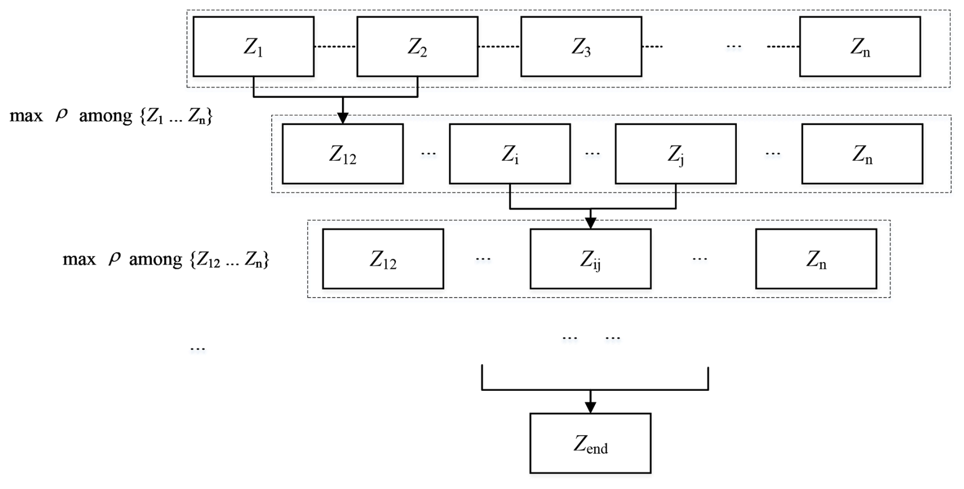
Failure events are combined pairwise in sequence until the n failure events $E_{\mathrm{1}},\mathrm{\dots },E_n$ with $E_i=\mathit{\{}{Z}_i\le \mathrm{0}\mathit{\}}$ are reduced to a single equivalent limit state Z_end, as shown in Fig. 1, with the associated failure event $E_{\mathrm{end}}=\mathit{\{}{Z}_{\mathrm{end}}\le \mathrm{0}\mathit{\}}$. The time-dependent failure probability over [t_s,t_e] is approximated by

$$\begin{array}{}\text{(23)}& p_{\mathrm{f}}(t_{\mathrm{s}},t_{\mathrm{e}})\approx \mathrm{Pr}\left(E_{\mathrm{end}}\right)=\mathrm{1}-\mathrm{\Phi }\left({\mathit{\beta }}_{\mathrm{end}}\right).\end{array}$$

Since each compounding step introduces an approximation, the final time-dependent failure probability may depend on the compounding order, and the approximation error can accumulate through subsequent steps (Roscoe et al., 2015). To reduce this order sensitivity, we repeatedly select the remaining pair with the largest correlation ρ_ij, compound the selected pair into a new equivalent event, update the correlations involving the new event, and continue until the final equivalent event E_end is obtained.

4 Numerical examples and discussion

4.1 Supported steel beam

4.1.1 Problem definition and solutions

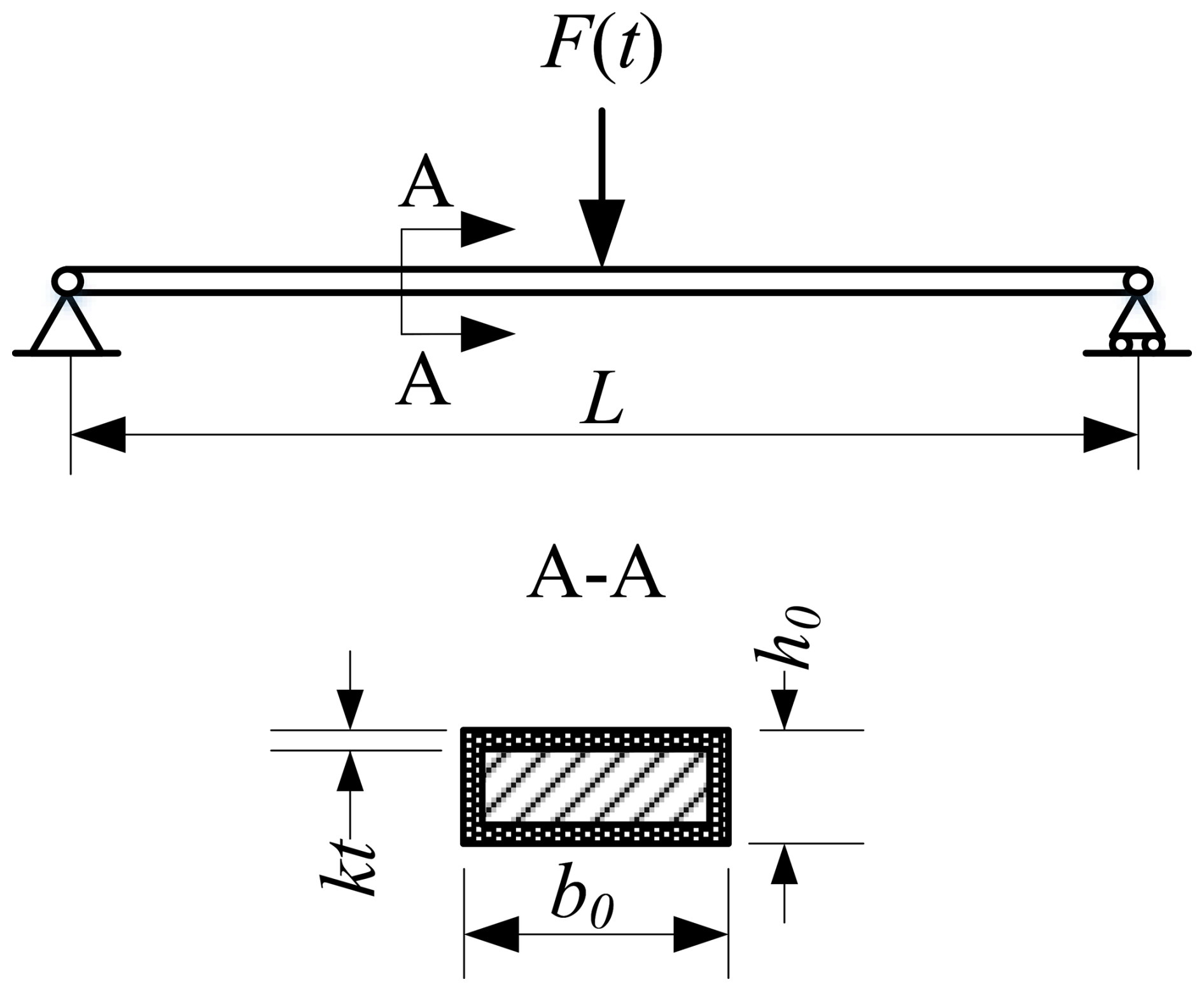
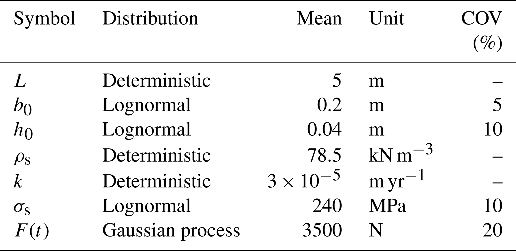
The supported steel beam shown in Fig. 2 is the most classic model of time-dependent reliability (Andrieu-Renaud et al., 2004). The length of the beam is L, and the width and height of the rectangular section are b₀ and h₀, respectively. The unit weight of the steel beam is ρ_s, and the force of the weight p=ρ_sb₀h₀ can be regarded to be a fixed uniform load acting on the beam. The time-dependent load is a concentrated force F(t) applied at the midspan. The steel beam is assumed to be complete at initial time t=0. The corrosion of the rectangular section is recognized as uniform, and the corrosion rate is denoted as k. The cross-section width and height with time are $b\left(t\right)=b_{\mathrm{0}}-\mathrm{2}kt$ and $h\left(t\right)=h_{\mathrm{0}}-\mathrm{2}kt$. The yield strength of the material is σ_s.

Figure 2 The model of the supported steel beam.

The autocorrelation function of the Gaussian process F(t) is defined as

$$\begin{array}{}\text{(24)}& \mathit{\rho }(t_i,t_j)=\exp \left[-{\left({\displaystyle \frac{|t_j-t_i|}{{\mathrm{\ell }}_{\mathrm{c}}}}\right)}^{\mathrm{2}}\right],\end{array}$$

where the correlation coefficient depends on the time lag $|t_j-t_i|$. The correlation length is set to ℓ_c=1 year in this example.

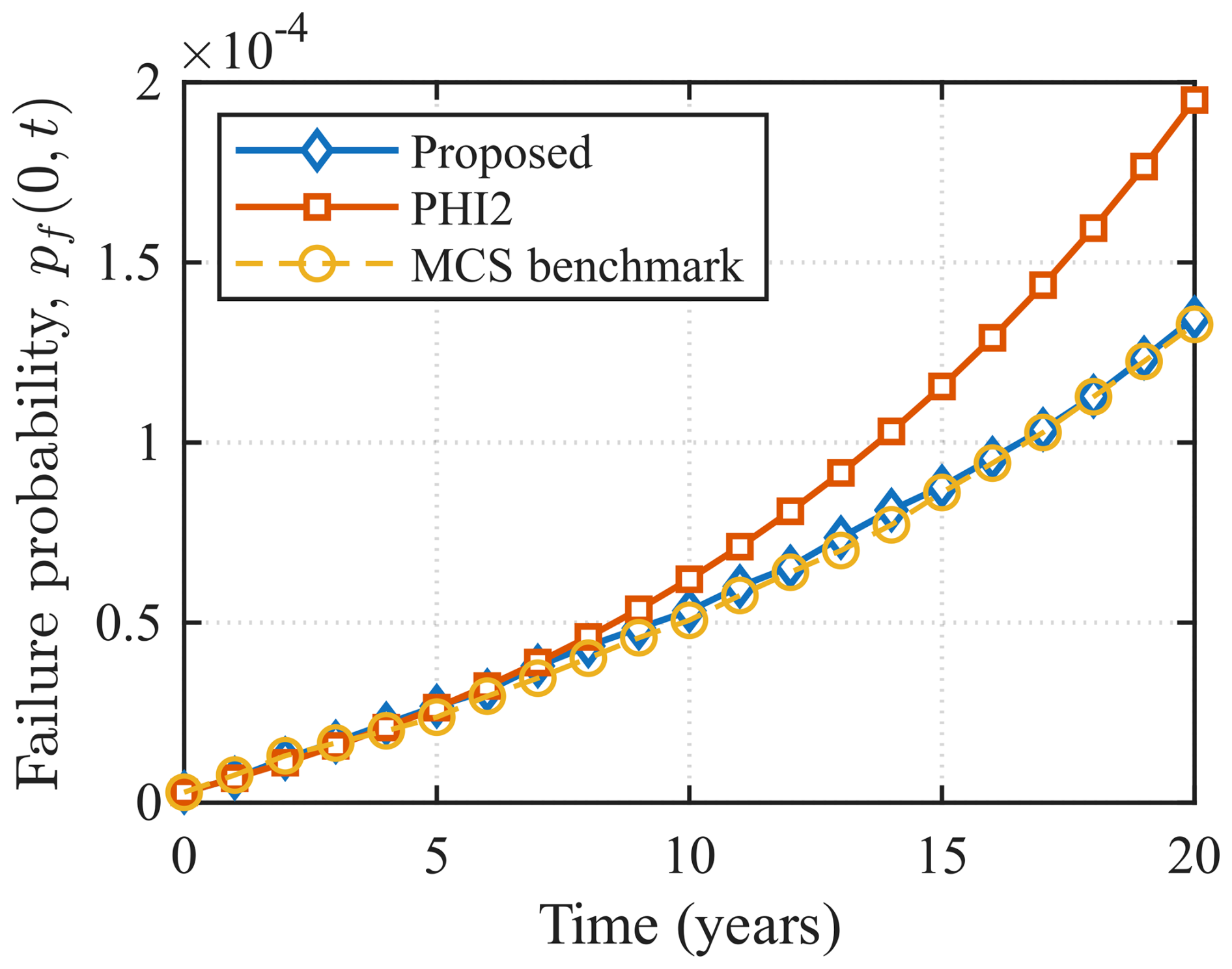
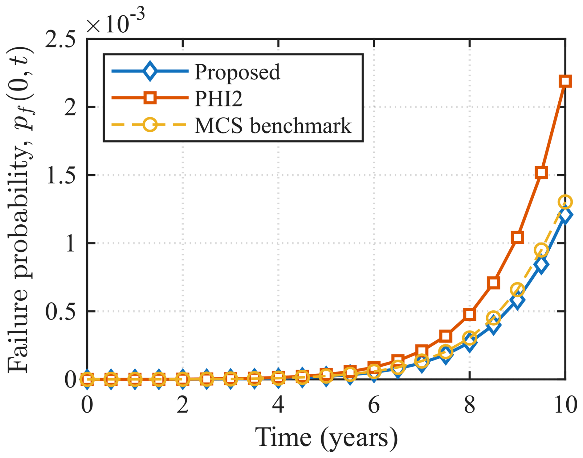
The statistical properties of all inputs are summarized in Table 1. The stochastic process over $t\in [\mathrm{0},\mathrm{20}]$ years is discretized into n=100 time instants for the proposed and PHI2 methods. In the proposed method, the EOLE truncation order is set to M=28 to ensure that the maximum pointwise approximation error over $t\in [\mathrm{0},\mathrm{20}]$ years does not exceed 1 %. For the MCS method, the stochastic process is discretized into n_MCS=500 time instants, and 10⁸ sample paths are simulated. The result of the MCS method is regarded to be the benchmark, and the results obtained by the proposed method and PHI2 are compared with the MCS benchmark in Fig. 3.

Table 1 Parameters of the corroded steel beam.

Figure 3 Failure probability of the steel beam with different methods.

Here, the error of the proposed and PHI2 methods is defined as

$$\begin{array}{}\text{(25)}& \mathit{\epsilon }(t_{\mathrm{s}},t_{\mathrm{e}})={\displaystyle \frac{\left|p_{\mathrm{f}}(t_{\mathrm{s}},t_{\mathrm{e}})-p_{\mathrm{f},\mathrm{MCS}}(t_{\mathrm{s}},t_{\mathrm{e}})\right|}{p_{\mathrm{f},\mathrm{MCS}}(t_{\mathrm{s}},t_{\mathrm{e}})}}\times \mathrm{100}\mathit{\%},\end{array}$$

where p_f(t_s,t_e) is the time-dependent failure probability over [t_s,t_e] estimated by the proposed method or PHI2, and $p_{\mathrm{f},\mathrm{MCS}}(t_{\mathrm{s}},t_{\mathrm{e}})$ is the corresponding estimate obtained by the MCS method.

Table 2 Failure probability of the steel beam over different periods.

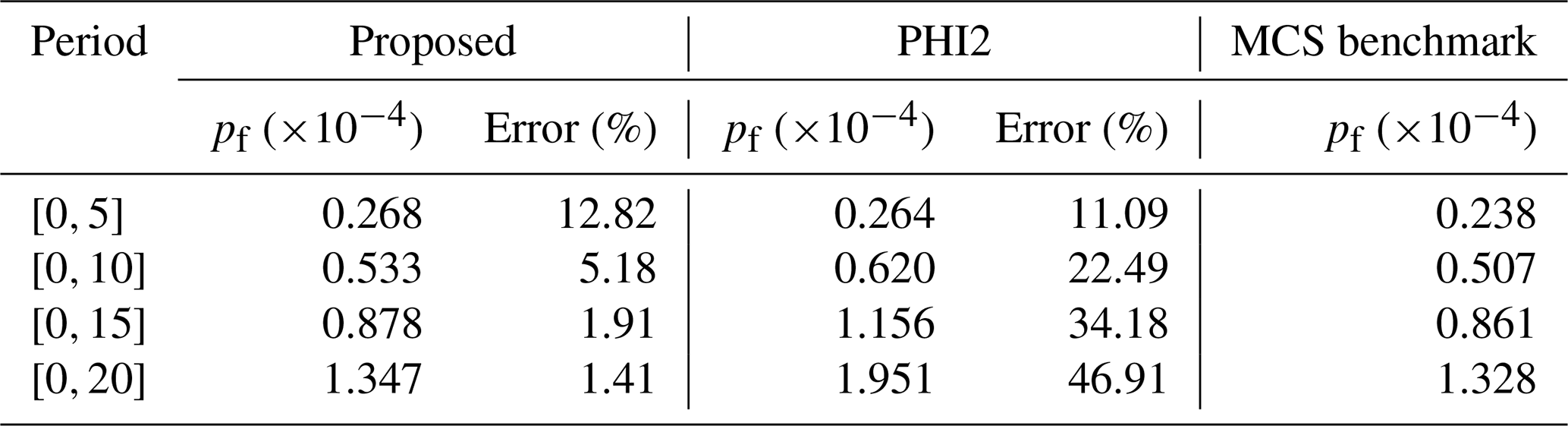
For $t_{\mathrm{e}}=[\mathrm{5},\mathrm{10},\mathrm{15},\mathrm{20}]$ years, the comparison is provided in Table 2. The result of the proposed method shows good agreement with the MCS benchmark, with a maximum relative error of 12.82 % over the considered time periods. In contrast, the relative error of the PHI2 method increases rapidly with time, reaching a maximum value of 46.9 %. In terms of the function calls, the MCS benchmark corresponds to 5×10¹⁰ calls. The proposed and PHI2 methods require 2.45×10⁴ and 4.328×10⁴ calls, respectively. The proposed method is more effective than the PHI2 and MCS methods.

4.1.2 Convergence and sensitivity analyses

i. Sensitivity to the time discretization level n

As the number of time discretization points n increases, the failure event over a continuous time period can be approximated on a finer temporal grid, thereby reducing the time discretization error. On the other hand, the EPA approximates the high-dimensional joint failure probability through repeated compounding of two events. It has been reported that, when the number of component events is large, the approximation error and the sensitivity to the compounding order may accumulate across multiple compounding levels so that the resulting system failure probability tends to be biased on the conservative side (Roscoe et al., 2015). Therefore, the choice of n should balance the time discretization error against the system-compounding error.

In the proposed method, a correlation-based compounding rule is adopted (see Fig. 1) to reduce order sensitivity and alleviate error accumulation. To investigate the influence of the discretization level on numerical stability and conservatism, the time period is discretized with n ranging from 30 to 400. For each n, the EOLE truncation order M is determined adaptively following the same criterion as in Sect. 4.1.1. The resulting time-dependent failure probability p_f(0,20) as a function of n is shown in Fig. 4. The MCS benchmark $p_{\mathrm{f},\mathrm{MCS}}(\mathrm{0},\mathrm{20})=\mathrm{1.328}\times {\mathrm{10}}^{-\mathrm{4}}$ is also plotted for comparison, together with a ±10 % band of $[\mathrm{1.195}\times {\mathrm{10}}^{-\mathrm{4}},\mathrm{1.461}\times {\mathrm{10}}^{-\mathrm{4}}]$. This band corresponds to an interval of reliability indices [3.6341, 3.6655], with Δβ≈0.03, indicating that a ±10 % variation in p_f at this probability level translates into only a minor change in β.

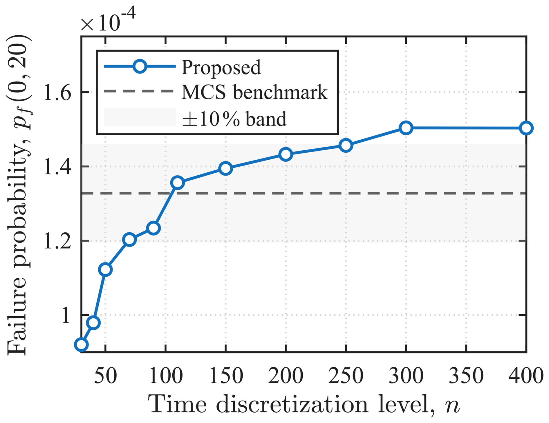
Figure 4 Convergence of the time-dependent failure probability with respect to the number of time discretization points n.

When n is small, the coarse temporal grid provides insufficient coverage of potential failure events within the considered time period, leading to an underestimated time-dependent failure probability. As n increases, more potential failure instants are captured, and time-dependent failure probability increases and gradually stabilizes. Once n≥70, the results enter the ±10 % band around the MCS benchmark. With further refinement, the variation of the time-dependent failure probability becomes limited; meanwhile, as the number of discretized events increases, the influence of system-compounding error on the final estimate becomes more pronounced, which may still cause an upward drift in failure probability. Throughout this study, the adaptively selected EOLE truncation order varies only within a narrow range of M≈28–31, suggesting that, under the current error threshold, M is relatively insensitive to the choice of n.

Based on the behavior of time-dependent failure probability in Fig. 4, a discretization level of approximately $n=[\mathrm{90},\mathrm{150}]$ is found to provide a good overall performance for this example. The corresponding time step is Δt≈0.225–0.134 years, and the correlation between two adjacent time instants is ρ(Δt)≈0.95–0.98 according to Eq. (24). Accordingly, this correlation range is adopted as the discretization guideline in the subsequent analyses.

ii. Sensitivity to the EOLE truncation order M

The EOLE truncation order M determines the fidelity with which the stochastic process Y(t) is represented in the finite-dimensional standard normal space. To examine its influence on the time-dependent failure probability, the time interval of $[t_{\mathrm{s}},t_{\mathrm{e}}]=[\mathrm{0},\mathrm{20}]$ years is discretized with a fixed level n=100, and M is varied from 5 to 80. The resulting failure probability over [t_s,t_e] is shown in Fig. 5. In this figure, the dashed line denotes the MCS benchmark $p_{\mathrm{f},\mathrm{MCS}}(\mathrm{0},\mathrm{20})=\mathrm{1.328}\times {\mathrm{10}}^{-\mathrm{4}}$, and the shaded region indicates a ±10 % band around this benchmark.

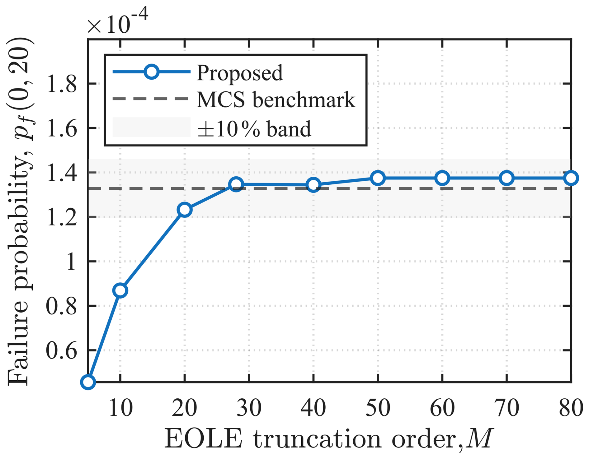
Figure 5 Convergence of the time-dependent failure probability with respect to the EOLE truncation order M.

As shown in Fig. 5, the estimate exhibits a pronounced sensitivity to M at low truncation orders. For M<20, the time-dependent failure probability is notably lower than the benchmark and increases rapidly with M, indicating that the truncated expansion is insufficient to preserve the process fluctuations that govern the occurrence of failure within the considered period. When M increases to approximately 20–40, the estimate approaches the benchmark and falls within the ±10 % band. For M≥50, the curve reaches a clear plateau, and further increasing M produces negligible changes in the time-dependent failure probability, demonstrating diminishing returns from higher truncation orders.

To relate this behavior to the truncation quality, the maximum pointwise error is reported as ${\mathit{\epsilon }}_{max}={max}_{j=\mathrm{1},\mathrm{\dots },n}\mathit{\epsilon }\left(t_j\right)$. The corresponding trend of ε_max with M is shown in Fig. 6. The results show an orders-of-magnitude decay of ε_max with increasing M. ${\mathit{\epsilon }}_{max}=\mathrm{1.21}\times {\mathrm{10}}^{-\mathrm{1}}$ at M=20, which is consistent with the marked underestimation observed in Fig. 5. At M=28, ε_max decreases to $\mathrm{9.65}\times {\mathrm{10}}^{-\mathrm{3}}$, and the corresponding time-dependent failure probability estimate is already close to the benchmark. Further increasing M reduces ε_max to the order of 10⁻⁷ or smaller, whereas the change in failure probability remains negligible.

Figure 6 The maximum pointwise EOLE truncation error with respect to M.

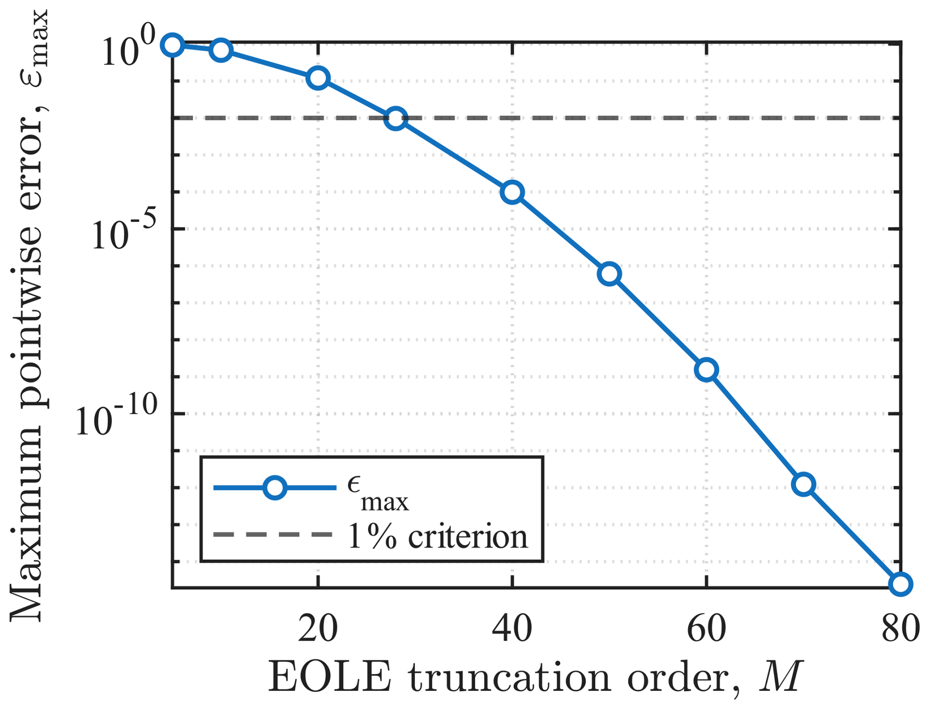
Taken together, Figs. 5 and 6 suggest that controlling the maximum pointwise error at the 1 % level is sufficient to obtain a practically stable estimate of time-dependent failure probability for this example. Tightening the threshold to 10⁻³ or 10⁻⁴ would substantially increase the process dimension while yielding only marginal changes in failure probability. Accordingly, M is chosen as the smallest truncation order satisfying ${\mathit{\epsilon }}_{max}\le \mathrm{1}$ % in the subsequent analyses.

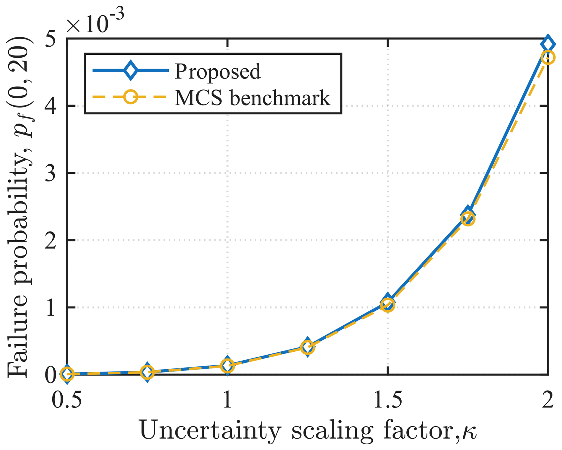
iii. Failure probability versus uncertainty level

To investigate the influence of the uncertainty level of the stochastic load process on the time-dependent failure probability, an uncertainty scaling factor κ is introduced to proportionally scale the standard deviation of the load process F(t). The mean function and correlation structure of F(t) remain the same as those in Sect. 4.1.1. The considered time period $t\in [\mathrm{0},\mathrm{20}]$ years is discretized with n=100 time instants, and the EOLE truncation order is selected adaptively using the same 1 % pointwise error criterion. A parametric scan is conducted over $\mathit{\kappa }\in [\mathrm{0.5},\mathrm{2.0}]$, and the proposed results are compared against an MCS benchmark with 10⁸ sample paths.

As shown in Fig. 7, the time-dependent failure probability p_f(0,20) increases markedly with the uncertainty scaling factor κ. For instance, p_f(0,20) rises from $\mathrm{8.074}\times {\mathrm{10}}^{-\mathrm{6}}$ at κ=0.5 to $\mathrm{1.347}\times {\mathrm{10}}^{-\mathrm{4}}$ at κ=1.0 and reaches $\mathrm{4.915}\times {\mathrm{10}}^{-\mathrm{3}}$ at κ=2.0, indicating that amplifying the load fluctuations markedly increases the likelihood of failure within the considered period. The proposed method closely follows the MCS benchmark across the entire range of κ, reproducing both the monotonic trend and the magnitude. The largest relative discrepancy is observed at κ=2.0, where the maximum relative error is about 4.15 %, corresponding to a small reliability index difference of $\left|\mathrm{\Delta }\mathit{\beta }\right|<\mathrm{0.015}$, which confirms the robustness of the proposed estimate under varying process uncertainty.

Figure 7 Failure probability versus uncertainty level.

4.2 The 23-bar truss

An elastic 23-bar truss (Baroth et al., 2011) is depicted in Fig. 8. The upper and lower chords have Young's modulus E₁ and cross-sectional area A₁, whereas the web members have Young's modulus E₂ and cross-sectional area A₂. The overall length of the truss is 24 m, and the height is 2 m. The external loads P_i(t) $(i=\mathrm{1},\mathrm{\dots },\mathrm{6})$ are assumed to share the same stationary Gaussian process P(t). The autocorrelation function is defined as

$$\begin{array}{}\text{(26)}& \mathit{\rho }\left(t_i,t_j\right)=\exp \left(-{\displaystyle \frac{|t_j-t_i|}{\mathrm{2}}}\right).\end{array}$$

Figure 8 The model of 23-bar truss structure.

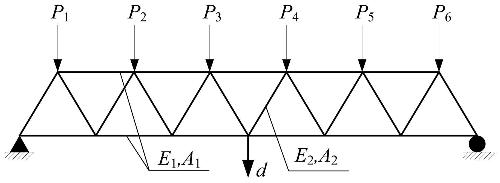
The serviceability requirement is that the maximum displacement does not exceed the allowable value d_max, and the limit state function is expressed as

$$\begin{array}{}\text{(27)}& G(\mathbf{X},P(t\left)\right)=d_{max}-d(\mathbf{X},P(t\left)\right),\end{array}$$

where d(X,P(t)) is the maximum displacement of the truss, and $d_{max}=\mathrm{13}$ cm is the maximum allowable displacement. The probabilistic characteristics of all of the parameters of the truss are provided in Table 3.

Table 3 Parameters of the 23-bar truss.

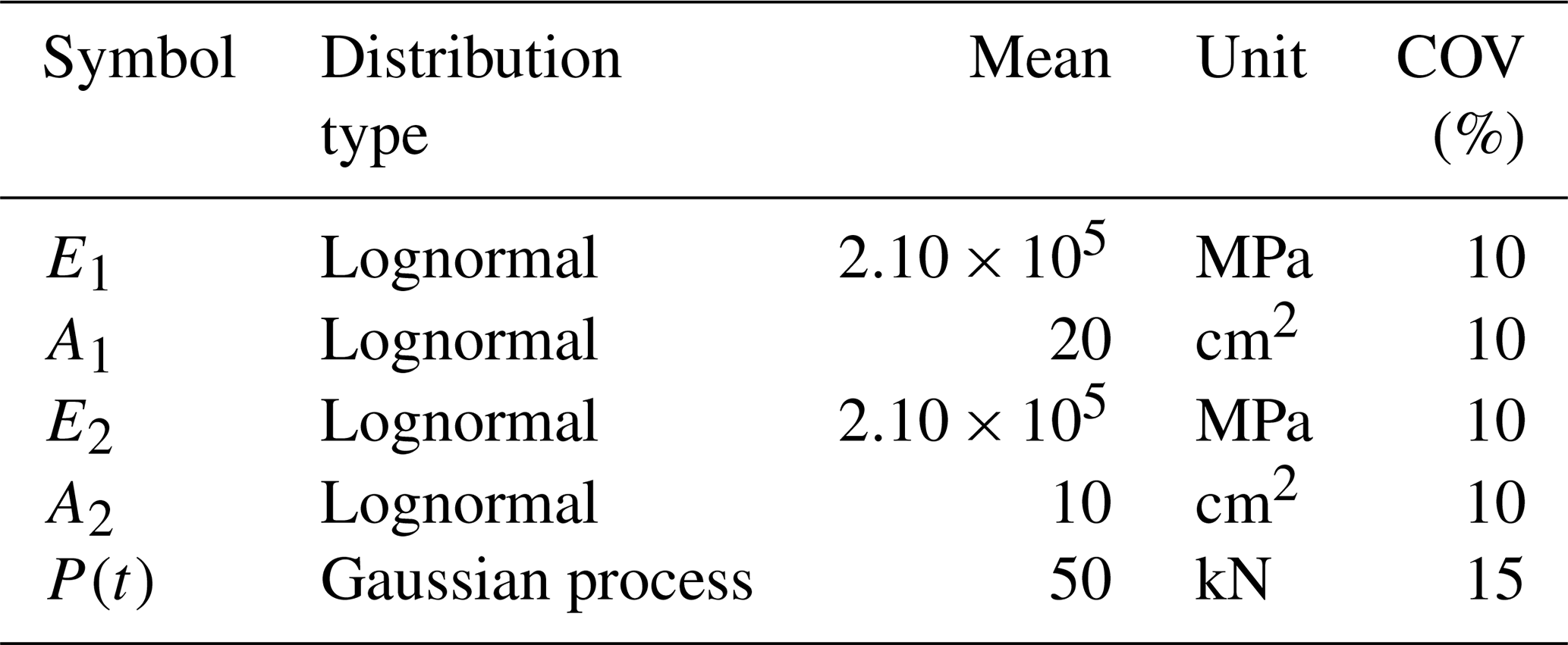
Table 4 Failure probabilities of the 23-bar truss over different periods.

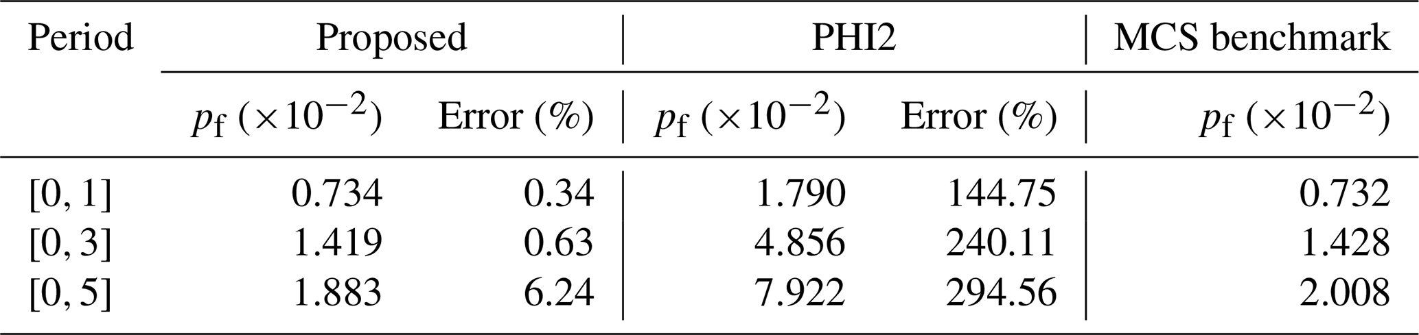
The time-dependent failure probability of the truss is considered over $t\in [\mathrm{0},\mathrm{5}]$ years. The stochastic load process is discretized into n=100 time instants for the proposed method. Because the load process is stationary and the model does not include any time degradation variable, the time-independent reliability problem is identical across all discretized instants. Hence, only one representative FORM analysis is required for the proposed method. In the proposed method, the FORM result at a representative time instant is used for all discretized time instants, and the EOLE truncation order is set to M=52 so that the pointwise approximation error of the load process is controlled within 1 % over the considered period. For PHI2, only a few FORM analyses are needed to estimate the outcrossing rate. For the MCS method, the stochastic process is discretized into n_MCS=200 time instants, and 1×10⁵ sample paths are simulated. Figure 9 and Table 4 compare the results of the proposed, MCS, and PHI2 methods. The proposed method agrees well with the MCS benchmark, and the maximum relative error over the considered periods is only 6.24 %. Meanwhile, the PHI2 method is unsuitable for this problem and has a maximum relative error of about 295 %. In terms of limit state function evaluations, the MCS benchmark needs 2×10⁷ calls, PHI2 requires 563 calls, and the proposed method requires only 168 calls.

Figure 9 Failure probabilities of the 23-bar truss with different methods.

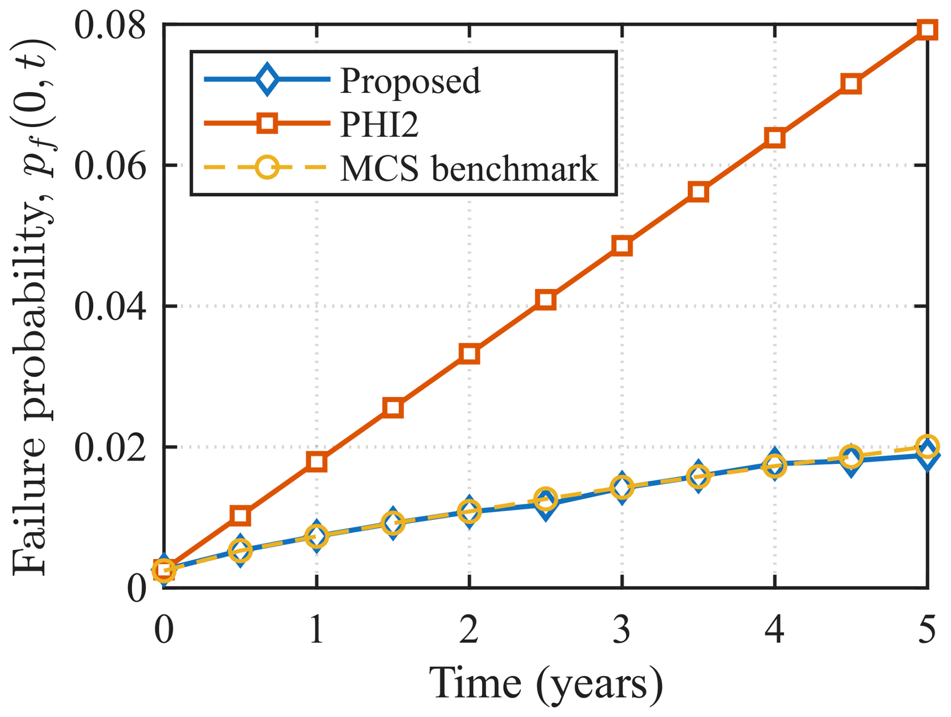
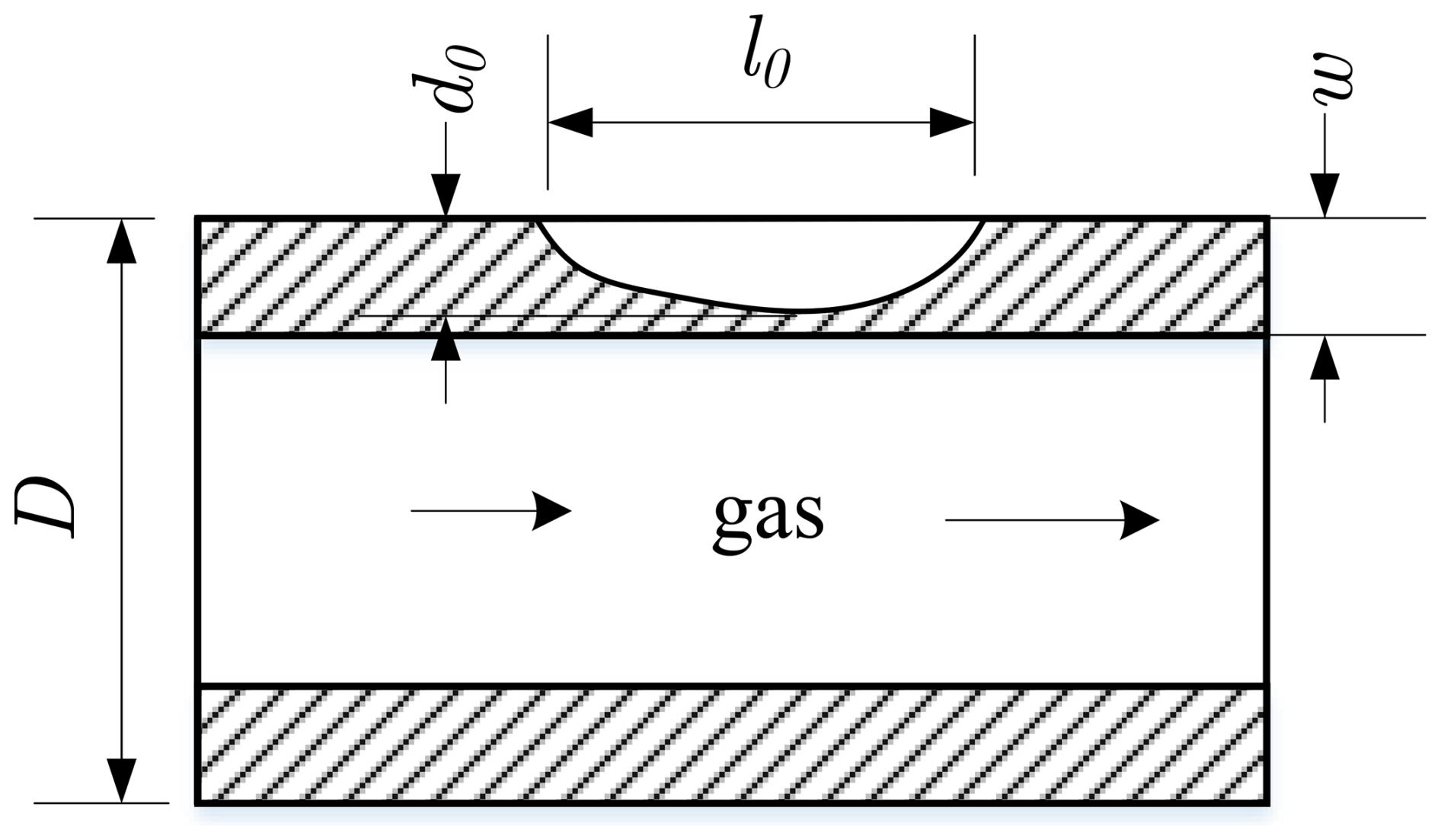
4.3 Corroded pipeline

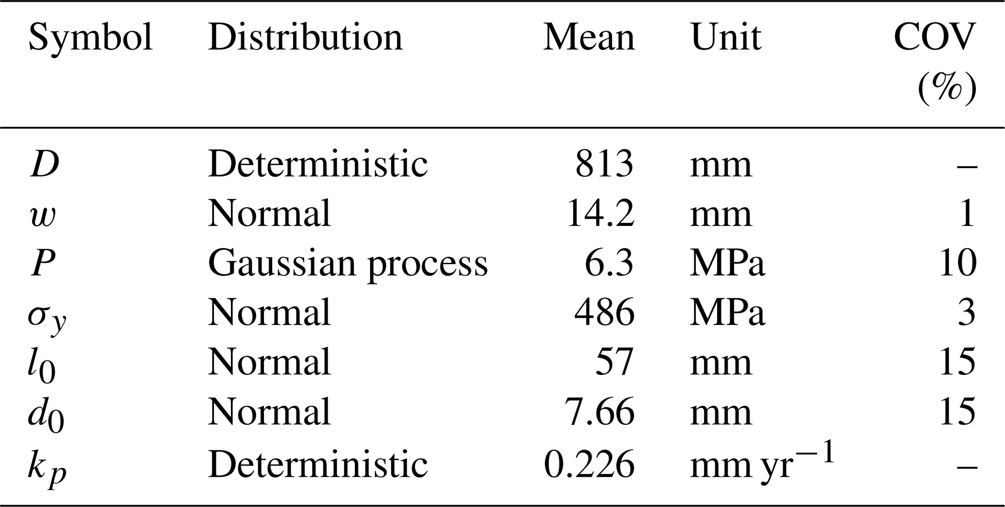
The buried natural-gas pipeline is subjected to both environmental corrosion and time-varying internal pressure. The internal pressure of the pipeline should be considered to be a stochastic process because it changes with time. The case study considers an in-service natural-gas pipeline located in eastern China. The pipeline is made of X65 steel with an outer diameter of D=813 mm and a wall thickness of w=14.2 mm, and the operating pressure is 6.3 MPa. The most recent in-line inspection (ILI) reported a dominant corrosion metal loss defect with a maximum depth of d₀=7.66 mm and an axial length of l₀=57 mm (see Fig. 10). In Fig. 10, the metal loss defect is idealized by its axial extent l₀ and the maximum wall thickness loss d₀ reported by the ILI. Based on the historical inspection records, an average corrosion growth rate of k_p=0.226 mm yr⁻¹ is adopted. The parameters of the pipeline and the defect are provided in Table 5.

Figure 10 The model of the corroded pipeline.

Table 5 Parameters of the corroded natural-gas pipeline.

The limit state function of a pipeline is defined as

$$\begin{array}{}\text{(28)}& G(\mathbf{X},t)=P_{\mathrm{b}}\left(t\right)-P\left(t\right),\end{array}$$

where P(t) is the operating pressure, and P_b(t) is the burst pressure.

The operating pressure is modeled as a stationary Gaussian process with the autocorrelation function given in Eq. (24), where ℓ_c=0.2 years for this case. The burst pressure is related to the structure, material, and defect state of the pipeline, which can be obtained by using the semi-empirical formula of ASME B31G (ASME, 2023),

$$\begin{array}{}\text{(29)}& P_{\mathrm{b}}\left(t\right)=\mathrm{2}\left({\mathit{\sigma }}_y+\mathrm{68.95}\right)\left({\displaystyle \frac{w}{D}}\right)\left[{\displaystyle \frac{\mathrm{1}-\frac{d\left(t\right)}{w}}{\mathrm{1}-\frac{d\left(t\right)}{wM\left(t\right)}}}\right],\end{array}$$

and Folias factor M(t) is

$$\begin{array}{}\text{(30)}& \begin{array}{rl}& M\left(t\right)=\\ & \left\{\begin{array}{ll}\sqrt{\mathrm{1}+\mathrm{0.6275}\frac{l(t{)}^{\mathrm{2}}}{Dw}-\mathrm{0.003375}\frac{l(t{)}^{\mathrm{4}}}{(Dw{)}^{\mathrm{2}}}},& \frac{l(t{)}^{\mathrm{2}}}{Dw}\le \mathrm{50}\\ \mathrm{0.032}\frac{l(t{)}^{\mathrm{2}}}{Dw}+\mathrm{3.3},& \frac{l(t{)}^{\mathrm{2}}}{Dw}>\mathrm{50}\end{array}\right.,\end{array}\end{array}$$

where the σ_y, w, and D are the yield strength, wall thickness, and outer diameter of the pipeline, respectively, and d(t) and l(t) are the defect depth and length at t, respectively.

Corrosion growth is modeled by a linear law and is predicted under a widely used engineering assumption that the depth-to-length ratio is preserved during growth (Carr, 2014). Accordingly,

$$\begin{array}{}\text{(31)}& \left\{\begin{array}{l}d\left(t\right)=d_{\mathrm{0}}+k_{p}t,\\ l\left(t\right)=l_{\mathrm{0}}\left(\mathrm{1}+\frac{k_p}{d_{\mathrm{0}}}t\right),\end{array}\right.\end{array}$$

where k_p is the average corrosion growth rate inferred from historical inspection records.

Table 6 Failure probabilities of the corroded pipeline over different periods.

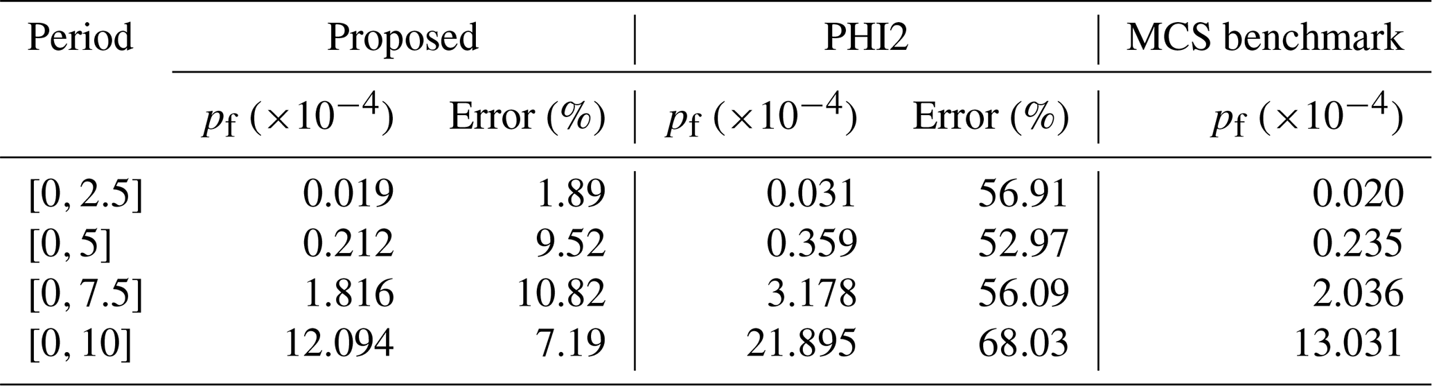
The time-dependent failure probability of the corroded pipeline is evaluated over $t\in [\mathrm{0},\mathrm{10}]$ years after the most recent ILI. The evaluation period is discretized into n=270 time instants for the proposed method, and the EOLE truncation order is chosen as M=69 so that the maximum pointwise approximation error over the period does not exceed 1 %. The PHI2 method is evaluated on the same time grid to obtain the time-dependent failure probability. The failure probabilities of the corroded pipeline using the three methods are compared in Fig. 11. The error comparison at different periods is provided in Table 6. In the MCS simulation, the pressure process is discretized at n_MCS=500 time instants, and 1×10⁸ sample paths are simulated. The proposed method agrees well with the MCS benchmark, and the maximum relative error over the considered period is 10.82 %. Meanwhile, PHI2 yields larger discrepancies and has a maximum relative error of 68.03 %. In terms of limit state function calls, the proposed method requires 3.59×10⁴ calls, whereas PHI2 requires 1.08×10⁶ calls. The MCS benchmark corresponds to 5×10¹⁰ calls.

Figure 11 Failure probability of corroded pipeline with different methods.

5 Conclusions

A new time-dependent reliability analysis method is presented in this work. This method employs FORM, EOLE, and EPA. FORM is used to analyze the reliability at each time instant. EOLE is used to represent the stochastic process by series expansion and to construct its correlated representation in the standard normal space, which supports the subsequent system aggregation over discretized time instants. EPA is employed to estimate the time-dependent failure probability of the series system over the considered period. Three numerical examples demonstrate the efficiency and accuracy of the proposed method. The results of the proposed method achieve close agreement with MCS benchmarks while requiring orders-of-magnitude fewer limit state evaluations. Compared with the PHI2 method, the proposed approach provides consistently improved accuracy in the studied examples.

Nevertheless, we also noted some limitations of the proposed method during this study. EPA inevitably introduces approximation errors when progressively compounding multiple failure events. When the stochastic process has a short correlation length and the response exhibits high-frequency fluctuations, a smaller time step is required to maintain adequate temporal resolution, which increases the number of compounding levels and may aggravate error accumulation and the sensitivity to the compounding order. For non-Gaussian stochastic processes, the dependence among time instants cannot be fully characterized by a correlation coefficient alone, and Gaussian approximations may lead to noticeable bias in tail probability estimates. Moreover, when the limit state function is strongly nonlinear, the first order linearization error of FORM may become non-negligible and can be further amplified through multi-aggregation. Future work will focus on mitigating these issues and improving the robustness of the method.