Solution of inverse geometrico-static problem (IGP) for suspended rigid-flexible coupling parallel mechanism (RFCPM) driven by elastic thin rods

Rigid-flexible coupling is the development trend of lightweight parallel mechanisms. Different from traditional rigid parallel mechanisms, although the flexible components are light in weight, the large elastic deformation generated by the mechanism will affect the precision and stability of the movement. The elastic deformation of the flexible components makes the kinematic modeling challenging, which limits the application and promotion of such mechanisms. To solve the kinematic problems of such mechanisms and improve motion accuracy, this paper takes the rigid-flexible coupling parallel mechanism driven by elastic thin rods as the research object, proposes an inverse geometrico-static problem (IGP) solution, and conducts relevant motion tests to verify the correctness of the solution. Firstly, to solve the geometric relationship between the elastic thin rods and the end of the mechanism during the motion of the mechanism, the rigid-flexible coupling parallel mechanism driven by the elastic thin rods is rigidified and equivalent to a four-cable traction parallel robot, and the rationality of the rigidification equivalence is analyzed. Secondly, the kinematic/static coupling problem (geometrico-static problem) of the four-cable parallel robot is solved by the numerical iteration method, and a simulation example is analyzed, which shows that the cable length and Euler angle are cosine-like functions, the center of gravity distance is negatively correlated with the Euler angle amplitude, and the height and gravity of the end effector are independent of it. Thirdly, for the inverse kinematics problem of the rigid-flexible coupling parallel mechanism driven by elastic thin rods, a method combining the planar chain beam model and the kinematic model of the four-cable parallel robot is proposed. Finally, two experimental platforms are built to test and verify the accuracy of the above kinematic models. The test of the four-cable robot shows that the Fréchet distances of the target trajectories and the actual trajectories are relatively small (near 1), and the test of the rigid-flexible coupling parallel mechanism shows that the maximum errors between the target trajectories and the actual trajectories are all no more than 1.5 mm. The results all indicate that the target trajectories and the actual trajectories are highly consistent, which proves that the models and numerical iterative method are highly accurate. The method proposed in this paper can effectively solve the IGP of similar mechanisms and provide theoretical support for its practical application.

1 Introduction

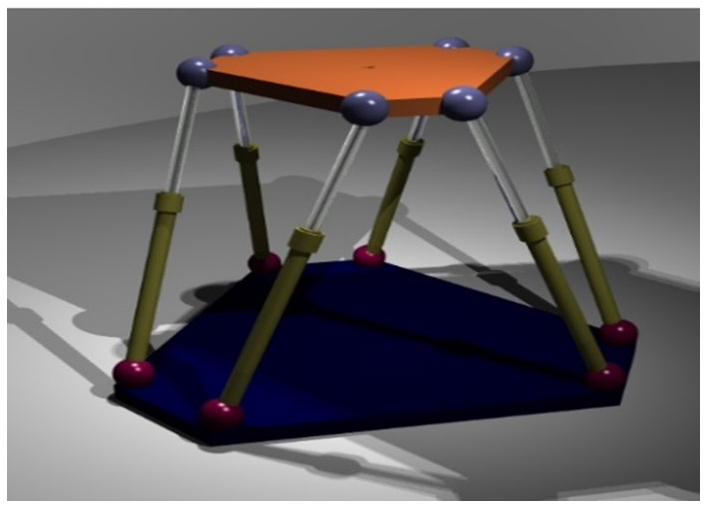
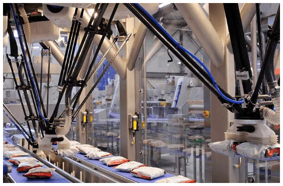
The parallel mechanism (as shown in Fig. 1) is a mechanism in which the end effector is driven by multiple kinematics chains connected to the base (Ye et al., 2020). It has the characteristics of strong load-bearing capacity, high accuracy, and fast speed (Zhang et al., 2022b; Tian et al., 2021) and is widely used in precision machining, high-speed sorting (as shown in Fig. 2), machine tools, farming tasks (Chhabra and Nagpal, 2023), and other fields. Although the traditional rigid parallel mechanism has many advantages, it also has some disadvantages: for example, the high stiffness makes it difficult for the end effector to ensure the safety and integrity of the object to be operated when interacting with the other object (Liu et al., 2020), and the heavy weight makes the inertia large during high-speed movement, which generates a large impact. People have increasingly high requirements for the speed and acceleration of the parallel mechanism. On the premise of ensuring the stability of robot movement, to improve the flexibility of parallel mechanism motion components and adaptability in different environments and to reduce the impact of inertia on dynamic characteristics, people gradually reduce the weight of motion components and improve the flexibility of components. Parallel mechanisms gradually evolve into rigid-flexible coupling parallel mechanisms (Zhang and Jiang, 2021). However, despite the soft or flexible characteristics of the motion components of the rigid-flexible coupling parallel mechanism, its modeling accuracy and accuracy are low (Mauze et al., 2020), and real-time performance cannot meet the control needs. This paper takes the rigid-flexible coupling parallel mechanism driven by elastic thin rods as the research object, rigidizes it to be equivalent to a cable parallel robot, and combines the kinematic model of the cable parallel robots with the modeling principle of a large-deformation elastic thin rod to accurately establish the inverse kinematic model of the original mechanism.

Figure 1 Rigid parallel mechanism.

Figure 2 High-speed sorting.

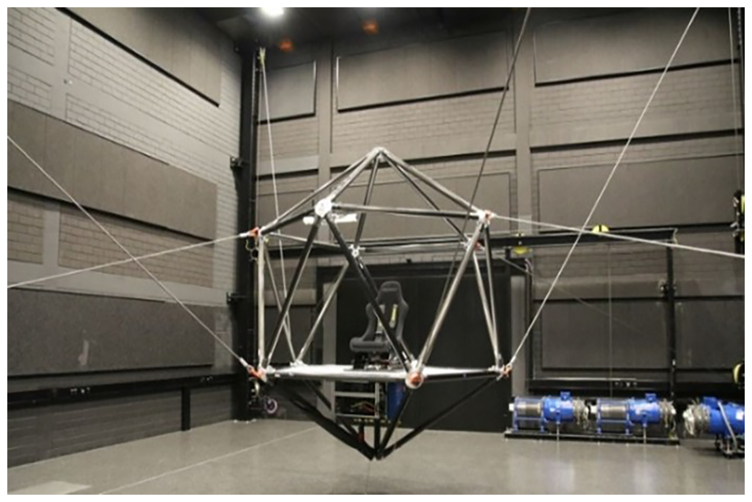
The cable robot is a rigid-flexible hybrid robot that uses flexible cables instead of rigid links to control the motion of the end effector, as shown in Fig. 3. It is usually composed of a fixed base, pulleys, winches, multiple cables, a drive connection base, and an end effector (Khoshbin et al., 2022). The cable is used to pull the actuator, and its principle includes controlling its length by connecting the cable to the moving platform and synchronously from the base frame through a winch (Iturralde et al., 2022). Compared with traditional rigid robots, it has the advantages of a large work space, small inertia (Zarebidoki et al., 2022), a higher payload–weight ratio (Qian et al., 2018), low cost (Zhang et al., 2022a), multiple functions (Paty et al., 2021), fast speed (Shang et al., 2020), and high acceleration (Bolboli et al., 2019).

Figure 3 Cable robot.

According to the quantitative relationship between the number of cables m and the number of degrees of freedom n, the constraint types of the cable-driven parallel robot (CDPR) can be divided into three categories: under-constrained ($m<n+\mathrm{1}$), fully constrained ($m=n+\mathrm{1}$), and over-constrained ($m>n+\mathrm{1}$). Among them, the motion of the under-constrained cable robot is uncertain, and its kinematic analysis and control are the core technical issues in application. How to efficiently solve the kinematic problem and achieve high-precision motion control is a research hotspot. The inverse geometrico-static problem (IGP) and direct geometrico-static problem (DGP) of the under-constrained cable parallel robots are currently unsolved classic problems, corresponding to their inverse kinematics and forward kinematics, respectively. IGP involves solving the length and tension of each cable given a part of the position or posture of the robot end. DGP involves calculating the posture and tension of the end given all the cable lengths corresponding to the robot end at any position.

In the under-constrained (suspended) configuration, gravity acts as a virtual cable, providing both geometric and force constraints. The position and posture of the end effector are determined by both the force and the length of the cable. The kinematic solution of under-constrained CDPRs is quite challenging. One of the main difficulties is that when given the length of the cable, the end effector retains some degrees of freedom and can still move, which may lead to some unpredictable oscillations (Ida et al., 2021). Therefore, the actual orientation is determined by the applied force. The intrinsic coupling between kinematics and statics of under-constrained CDPR is the biggest challenge in its kinematics static analysis. The closed-loop vector equation and the force system equilibrium equation must be solved simultaneously (Carricato and Merlet, 2012; Chen et al., 2024), which is much more complex than the displacement analysis of the fully constrained parallel robots with rigid links. This is usually because the cable can exert only a unilateral force, that is, it can only pull the end effector and cannot push it, so it is difficult to achieve static balance. Moreover, there may be multiple balanced and unstable states at the end of the under-constrained cable parallel robot. How to find a stable balanced configuration, find feasible solution sets of forward and inverse kinematics, and suppress unnecessary oscillation movements at the end are all challenging problems (Hwang et al., 2022). If the geometric static problem cannot be solved, kinematic analysis and kinematic control of such robots cannot be carried out, and it is difficult to apply these robots, as well as their kinematic analysis and control, in practice. The rigid-flexible coupling parallel mechanism driven by elastic thin rods studied in this paper also has the above characteristics of the cable robot.

For IGP, Carricato proposed an effective elimination procedure for under-constrained three-cable CDPRs, thereby obtaining a univariate polynomial without stray factors. Finally, all balanced configurations of the end effector were found (Carricato, 2013b), but the solution process is complicated, and no unique real solution is filtered out from all solutions.

For DGP, Carricato (Abbasnejad and Carricato, 2015; Carricato, 2013a) used a hybrid elimination method to obtain potential complete solutions for under-constrained CDPRs with different cable numbers (three cables, no more than six cables), but there are situations in the solution set in which not all cables are in a tension state. In order to find the upper limit of the number of complete solution sets, Abbasnejad used three numerical methods, that is, a continuous program, a genetic algorithm, and a particle swarm algorithm adapted via the algorithm proposed by Dietmaier, to find DGP with an under-constrained three-cable CDPR to provide up to 54 actual configurations (Abbasnejad and Carricato, 2012), but too many actual configurations are still difficult to use for real-time motion control of CDPRs. Berti et al. used interval analysis methods to solve DGP with no more than six cables and found all balanced configurations of the end effector but did not filter out the only actual configuration (Berti et al., 2016). Neural networks can be used for under-constrained four-cable CDPRs, over-constrained planar four-cable CDPRs, and even any other type of CDPR, having been used many times to solve the forward and inverse kinematics of CDPRs (Mishra and Caro, 2022; Chawla et al., 2023). However, neural networks need to process a large amount of data, have poor real-time performance, and are difficult to apply to real-time motion control.

So far, domestic and foreign scholars have made improvements and enhancements to the algorithm for solving the forward and inverse kinematics of the cable parallel robot. However, the algorithms currently proposed are still relatively complex and difficult to apply and promote. Therefore, this paper is dedicated to studying an intelligent and efficient algorithm to solve the inverse kinematics problem of the cable parallel robot. Regarding the kinematics problem of the rigid-flexible coupling parallel mechanism driven by elastic thin rods, in addition to solving the inverse kinematics problem of the equivalent cable parallel robot, the key lies in solving the kinematics problem of elastic thin rods, that is, establishing an accurate mathematical model to describe the relationship between the deformation and displacement of the continuum. Chen proposed a method for modeling the large plane deflection of the initial curved beam of a uniform cross-section (Chen et al., 2019), namely, the chained beam constraint model (CBCM), which can efficiently and accurately calculate the degree of geometric nonlinear large deformation of elastic thin rods. The planar chain beam model is an important model for studying the geometric nonlinear deformation of planar elastic thin rods in this paper.

This paper aims to study the inverse kinematics problem of a rigid-flexible coupling parallel mechanism driven by four elastic thin rods. By using the rigidification equivalent method, the mechanism is equivalent to a four-cable parallel robot (i.e., a rigidified equivalent mechanism). The IGP kinematic model of the four-cable parallel robot and the planar chain beam model are combined to obtain the inverse kinematic solution of the rigid-flexible coupling parallel mechanism.

The rest of this article is organized as follows: Sect. 2 analyzes the principle of rigidification equivalence and derives and simulates the inverse kinematics model of the rigidification equivalent mechanism. Section 3 introduces the chain beam model and assembles the chain beam model with the kinematic model of the rigidification equivalent four-cable parallel mechanism. Section 4 builds two test platforms to verify the accuracy of the inverse kinematics model of the rigidification equivalent mechanism and the original mechanism. The concluding remarks are made in the last section.

2 Materials and methods

2.1 Establishment and analysis of an equivalent four-cable drive model

The mechanism studied in this paper is shown in Fig. 4. The main function of this mechanism is to control the axial displacement of the elastic thin rod by driving the joint, thereby changing the position and pose of the end object in three-dimensional space and finally enabling the robot end to move along a given trajectory. To achieve this goal, after the position of the robot end is given, the lengths of the four elastic thin rods need to be solved. Although the position and rotation angle of the endpoint of the elastic thin rod are coupled, both are unknown quantities, which makes it quite challenging to directly perform large deformation analysis on the elastic thin rod.

To solve the inverse kinematics problem of the mechanism, the key is to solve the spatial position of the elastic thin rod and the four connection points at the end (which can also be regarded as the posture of the robot end). The common method to solve the position of the endpoints of the elastic thin rod after deformation is the pseudo-rigid body method. Drawing on the idea of the pseudo-rigid body model, the two ends of the elastic thin rod are connected to rigidify it into a tensioned cable. The rigid-flexible coupling parallel mechanism is rigidified to be equivalent to a four-cable suspended parallel robot. In the selection of rigid components, there are three reasons for choosing a cable instead of a rigid bar: (1) in general, the length of the rigid bar is fixed. Making the robot move requires choosing a drive with variable joint parameters, such as a cable with controllable cable length. (2) The rigid bar cannot reflect the suspension characteristics (IGP) of the elastic thin rod caused by gravity. (3) The choice of a rigid bar is not conducive to conducting experiments to verify the kinematic model.

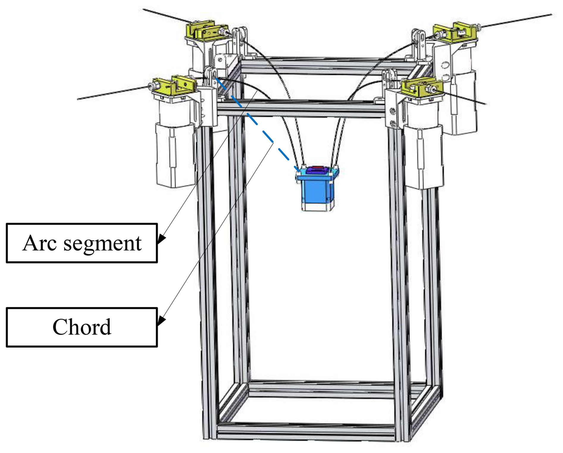
Figure 4 Relationship between the arc length and chord length of an elastic thin rod (rigidization equivalence).

The principle of rigidification equivalence is to equate the chord length of the elastic thin rod to a tensioned cable, ignoring the catenary model generated by the cable's own weight but equating the cable to an ideal straight line. Then, mathematical methods are used to find the mapping relationship between the cable length (the chord length at the endpoints of the elastic thin rod) and the arc length connecting the end of the elastic thin rod. Therefore, the kinematic model of the mechanism can be decomposed into the kinematic model of the four-cable driven parallel robot (Sect. 2.1.1) and the planar elastic thin rod model (Sect. 2.2.1).

2.1.1 Kinematics modeling of the four-cable parallel robot

The force analysis of the four-cable parallel robot is shown in Fig. 5. The number of cables m is 4, the number of controllable degrees of freedom (three mobile degrees of freedom) n is 3, and $m=n+\mathrm{1}$ is satisfied, which is a fully constrained configuration. The robot has the problem of kinematic and static coupling, which makes the kinematic solution very challenging. The IGP of the four-cable robot is to solve the posture of the end and the length of each cable by giving only the spatial coordinates of the endpoint E of the robot. Solving the motion posture of the end is the key to solving its inverse kinematics problem. The end posture is the result of gravity acting as a virtual cable and providing force constraints and geometric constraints at the same time. It can be seen that the statics and kinematics of the robot are coupled, and both must be solved at the same time.

Figure 5 Force analysis diagram.

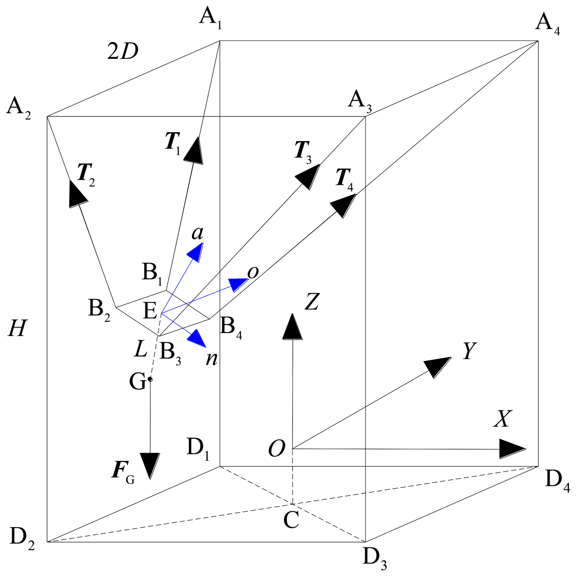
When the axis of the end is collinear with the Z axis and the bottom surface of the end is coplanar with the surface D₁D₂D₃D₄, establish a right-handed global coordinate system O−XYZ with the center of the end as the origin O (the projection of O on the bottom surface of the frame is point C, and $\left|OC\right|$ is the length of the end), the direction of A₁A₄ as the positive direction of the X axis, the direction of A₃A₄ as the positive direction of the Y axis, and the vertical upward as the positive direction of the Z axis. ${\mathit{T}}_i(i=\mathrm{1},\mathrm{2},\mathrm{3},\mathrm{4}$) is the tension vector of the cable at the end. The meaning of i in the following text is from 1 to 4, and it is assumed that each cable is in a tense state. F_G represents the gravity exerted on the center of gravity G at the end. Set the global coordinates of point $E(x_E,y_E,z_E)$ and the global coordinates of point $G\left(x_G,y_G,z_G\right)$. Define intermediate quantity $D=\left|{\mathbf{A}}_{\mathrm{1}}{\mathbf{A}}_{\mathrm{2}}\right|/\mathrm{2}$, and assume that half the length of the side of quadrilateral B₁B₂B₃B₄ is b, the distance from the center of gravity G to the quadrilateral B₁B₂B₃B₄ is L, and the height of the rack ($\left|A_{\mathrm{2}}{D}_{\mathrm{2}}\right|$) is H. When the top surface of the end is parallel to the plane XOY, let the distance from point O to plane A₁A₂A₃A₄ be h(h<H). Assume the mass of the robot end is m, the gravitational acceleration is g, and the end gravity F_G=mg.

During the movement of the end, the center point E of the quadrilateral B₁B₂B₃B₄ is taken as the origin of the moving coordinate system, the direction of B₂B₃ is the positive direction of the n axis, and the direction of B₂B₁ is the positive direction of the o axis. The right-handed coordinate system Enoa is established to describe the position and posture of the robot end when it moves in three-dimensional space. Set $\mathit{n}=[\mathrm{1},\mathrm{0},\mathrm{0}{]}^T\mathit{o}=[\mathrm{0},\mathrm{1},\mathrm{0}{]}^T$, and let $\mathit{a}=[\mathrm{0},\mathrm{0},\mathrm{1}{]}^T$ be the unit vectors along the n axis, o axis, and a axis, respectively; then, one can obtain

$$\begin{array}{}\text{(1)}& \left\{\begin{array}{l}\left|\mathit{n}\right|=\left|\mathit{o}\right|=\left|\mathit{a}\right|=\mathrm{1}\\ \mathit{n}\cdot \mathit{o}=\mathrm{0}\\ \mathit{n}\cdot \mathit{a}=\mathrm{0}\\ \mathit{o}\cdot \mathit{a}=\mathrm{0}\end{array}\right..\end{array}$$

Assume that the angle between EB₁ and n is θ_x1, the angle between EB₁ and o is θ_y1, the angle between EB₁ and a is θ_z1, and the angle between EB₁ and EG is θ_G1. The expressions are as follows:

$$\begin{array}{}\text{(2)}& \left\{\begin{array}{l}\cos {\mathit{\theta }}_{xl}=\frac{\mathit{E}{\mathit{B}}_{\mathrm{1}}\cdot \mathit{n}}{\left|\mathit{E}{\mathit{B}}_{\mathrm{1}}\right|\cdot \left|\mathit{n}\right|}=-\frac{\mathrm{1}}{\sqrt{\mathrm{2}}}\\ \cos {\mathit{\theta }}_{yl}=\frac{\mathit{E}{\mathit{B}}_{\mathrm{1}}\cdot \mathit{o}}{\left|\mathit{E}{\mathit{B}}_{\mathrm{1}}\right|\cdot \left|\mathit{o}\right|}=\frac{\mathrm{1}}{\sqrt{\mathrm{2}}}\\ \cos {\mathit{\theta }}_{zl}=\frac{\mathit{E}{\mathit{B}}_{\mathrm{1}}\cdot \mathit{a}}{\left|\mathit{E}{\mathit{B}}_{\mathrm{1}}\right|\cdot \left|\mathit{a}\right|}=\mathrm{0}\\ \cos {\mathit{\theta }}_{Gx}=\frac{\mathit{n}\cdot \mathit{E}\mathit{G}}{\left|\mathit{n}\right|\cdot \left|\mathit{E}\mathit{G}\right|}=\mathrm{0}\\ \cos {\mathit{\theta }}_{Gy}=\frac{\mathit{o}\cdot \mathit{E}\mathit{G}}{\left|\mathit{o}\right|\cdot \left|\mathit{E}\mathit{G}\right|}=\mathrm{0}\\ \cos {\mathit{\theta }}_{Gz}=\frac{\mathit{a}\cdot \mathit{E}\mathit{G}}{\left|\mathit{a}\right|\cdot \left|\mathit{E}\mathit{G}\right|}=-\mathrm{1}\end{array}\right..\end{array}$$

By analogy, calculate the cosine values of the angles between $\mathit{E}{\mathit{B}}_j(j=\mathrm{2},\mathrm{3},\mathrm{4})$ and n, o, and a, that is, cos θ_xj, cos θ_yj, and cos θ_zj, respectively. In addition, we have the following relations:

$$\begin{array}{}\text{(3)}& \left\{\begin{array}{l}\left|\mathit{E}{\mathit{B}}_i\right|=\sqrt{\mathrm{2}b}\\ \left|\mathit{E}\mathit{G}\right|=L\end{array}\right..\end{array}$$

In the moving coordinate system, it is easy to get the relative coordinates of B_i: B₁ (−b, b, 0), B₂ (−b, −b, 0), B₃ (b, −b, 0), and B₄ (b, b, 0). The unit vector of the tension along the cable is

$$\begin{array}{}\text{(4)}& {\mathit{e}}_i={\displaystyle \frac{{\mathit{B}}_i{\mathit{A}}_i}{\left|{\mathit{B}}_i{\mathit{A}}_i\right|}}.\end{array}$$

In the global coordinate system, the unit vector of gravity is ${\mathit{e}}_G=[\mathrm{0},\mathrm{0},-\mathrm{1}{]}^T$. Assume that the modulus of the tension of each cable is T_i and the modulus of gravity is F_G. When the robot end moves in three-dimensional space, according to the vector balance equation of force:

$$\begin{array}{}\text{(5)}& T_{\mathrm{1}}{\mathit{e}}_{\mathrm{1}}+T_{\mathrm{2}}{\mathit{e}}_{\mathrm{2}}+T_{\mathrm{3}}{\mathit{e}}_{\mathrm{3}}+T_{\mathrm{4}}{\mathit{e}}_{\mathrm{4}}+F_G{\mathit{e}}_G=\mathbf{0}.\end{array}$$

Use the posture matrix to describe the motion posture of the robot end. Assume that the posture matrix T of the robot end at any time can be expressed by the global unit vector:

$$\begin{array}{}\text{(6)}& \mathbf{T}=\left[\begin{array}{lll}{n}_x& o_x& a_x\\ n_y& o_y& a_y\\ n_z& o_z& a_z\end{array}\right]=\left[\begin{array}{lll}\mathit{n}& \mathit{o}& \mathit{a}\end{array}\right].\end{array}$$

Inside, $\mathit{n}=[n_x,n_y,n_z{]}^T$, $\mathit{o}=[o_x,o_y,o_z{]}^T$, and $\mathit{a}=[a_x,a_y,a_z{]}^T$.

Assume that the moment of force vector T_i on point E is M_i and the moment of gravity vector F_G on point E is M_G. The vector equilibrium equation according to the torque is

$$\begin{array}{}\text{(7)}& {\mathit{M}}_{\mathrm{1}}+{\mathit{M}}_{\mathrm{2}}+{\mathit{M}}_{\mathrm{3}}+{\mathit{M}}_{\mathrm{4}}+{\mathit{M}}_G=\mathrm{0}.\end{array}$$

Inside, ${\mathit{M}}_i=\mathit{E}{\mathit{B}}_i\times {\mathit{T}}_i$.

In the above kinematic and static equations, there are a total of 28 unknowns involved, including the moduli of the four tension vectors, the nine elements of the attitude matrix T, the global coordinate components of the cable pulling point B_i (a total of 12 unknowns here), and the three global coordinate components of the center of gravity G. The number of equations involved can be expanded to 32 by projection, including the six-unit vector relations in equation group (1), the five distance constraint equations in equation group (3), the 12 cosine expressions of the angles between O_iB_i and the moving system coordinate axes, the three cosine expressions of the angles between EG and the moving system coordinate axes in equation group (2), the three component expressions obtained by projecting Eq. (5) onto the XYZ axes, and the three component expressions obtained by projecting Eq. (7) onto the XYZ axes.

The number of equations is greater than the number of unknowns, but the number of independent equations is still less than the number of unknowns because some of the equations are coupled. This can be explained if Euler angles are used to represent the end effector's posture. At this time, there are a total of seven unknowns (four tension values and three posture angles), but the spatial force system equilibrium equation group has only six equations.

Combine the above equations and use the built-in fsolve function of MATLAB to iterate the coordinates of point B_i. When the end moves in space, the global coordinates of point B_i are set to $(x_{Bi},y_{Bi},z_{Bi})$. The matrix X consisting of the physical quantities to be calculated is constructed as follows:

$$\begin{array}{}\text{(8)}& \mathbf{X}={\left[\begin{array}{llllllllll}{n}_x& o_x& a_x& x_{B\mathrm{1}}& x_{B\mathrm{2}}& x_{B\mathrm{3}}& x_{B\mathrm{4}}& x_G& T_{\mathrm{1}}& T_{\mathrm{4}}\\ n_y& o_y& a_y& y_{B\mathrm{1}}& y_{B\mathrm{2}}& y_{B\mathrm{3}}& y_{B\mathrm{4}}& y_G& T_{\mathrm{2}}& \mathrm{0}\\ n_z& o_z& a_z& z_{B\mathrm{1}}& z_{B\mathrm{2}}& z_{B\mathrm{3}}& z_{B\mathrm{4}}& z_G& T_{\mathrm{3}}& \mathrm{0}\end{array}\right]}^T.\end{array}$$

Take an initial value for each physical quantity in X to form an initial value matrix X₀.

$$\begin{array}{}\text{(9)}& {\mathbf{X}}_{\mathrm{0}}={\left[\begin{array}{llllllllll}\mathrm{1}& \mathrm{0}& \mathrm{0}& x_E-b& x_E-b& x_E+b& x_E+b& x_E& mg/\mathrm{4}& mg/\mathrm{4}\\ \mathrm{0}& \mathrm{1}& \mathrm{0}& y_E+b& y_E-b& y_E-b& y_E+b& y_E& mg/\mathrm{4}& \mathrm{0}\\ \mathrm{0}& \mathrm{0}& \mathrm{1}& z_E& z_E& z_E& z_E& z_E-L& mg/\mathrm{4}& \mathrm{0}\end{array}\right]}^T\end{array}$$

Although the fsolve function needs to set the initial value of the equation group, is sensitive to the initial value, and returns only one solution result, considering that the robot end only corresponds to a unique posture when it is in any position in the three-dimensional space, as long as a reasonable initial value is given, this solution has high feasibility and can search for a unique and definite end posture. After iterating the coordinates of the B_i point, convert them into the posture angle of the robot end. Assume the rotation angle of the end around the n axis is α, the rotation angle of the end around the o axis is β, and the rotation angle of the end around the a axis is γ. The same iterative method can be used to solve the values of the three angles.

2.1.2 Simulation examples and analysis

In the mechanism studied in this paper, b=16, D=127, h=498, and L=38 mm are set. The point E at the end of the robot is controlled to move along a given circular trajectory. Two hundred points are taken at equal intervals on the circular trajectory, the configuration corresponding to each position point (physical quantities such as cable length and attitude angle) is calculated, and the changing laws of these physical quantities are analyzed.

Assume the parametric equation of the circular trajectory is (in mm)

$$\begin{array}{}\text{(10)}& \left\{\begin{array}{l}x=\mathrm{80}\cos \mathit{\theta }\\ y=\mathrm{80}\sin \mathit{\theta }\\ z=\mathrm{50}\end{array}\right..\end{array}$$

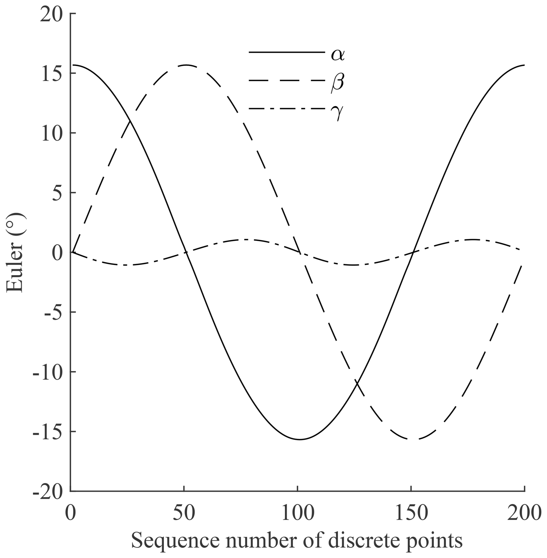
Inside, $\mathit{\pi }/\mathrm{2}\le \mathit{\theta }\le \mathrm{5}\mathit{\pi }/\mathrm{2}$. Before each movement, the robot starts from the position $\mathit{\theta }=\mathit{\pi }/\mathrm{2}$. If we look from the positive direction of the n axis, the rotation angle around the n axis is defined as positive in the counterclockwise direction and negative in the clockwise direction (both the o axis and the a axis are also defined in this way), and the attitude angle corresponding to each discrete point is connected into a smooth curve; then, the attitude angle change trend of the robot end during the movement along the circular trajectory (10) is as shown in Fig. 6. Among them, α, β, and γ are the rotation angles around the n axis, o axis, and a axis, respectively. The frame has a high degree of symmetry. When the robot end moves along the horizontal circular trajectory, the phase angles of α and β differ by 90°, and the maximum value and period are the same. The four cables exert force constraints on the robot end, making the rotation angle of the end around the a axis of the coordinate system very small and negligible.

Figure 6 Changes in the terminal Euler angle.

Figure 7 Cable length variation diagram.

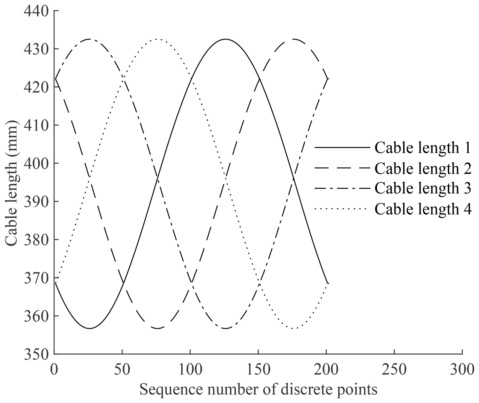
As shown in Fig. 7, the length of each cable is a quasi-sine function with the same amplitude and angular frequency and the same phase difference, which conforms to the symmetry of the circular trajectory.

Keep other physical quantities unchanged (such as L=38, r=80, b=16, and D=127 mm), only change the size of the vertical coordinate z_E of the endpoint E, and solve the amplitude α_m of the angle α corresponding to different heights, as shown in Fig. 8.

Figure 8 Relationship between terminal height and angle amplitude.

Figure 9 Relationship between L and α_m.

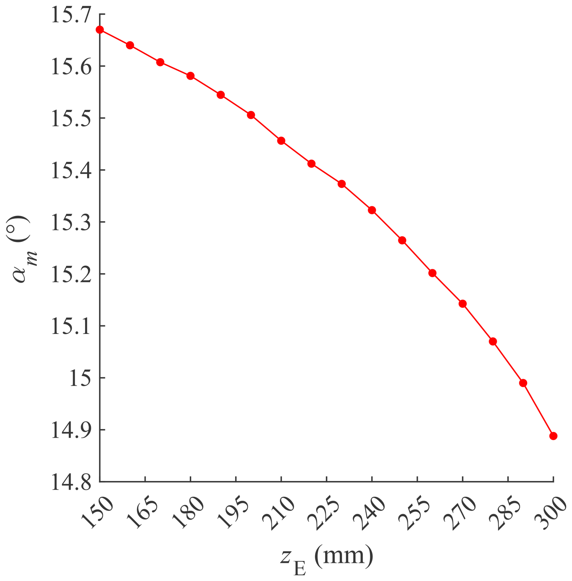
The changing relationship between the end height z_E and the angle amplitude α_m is not significant because the amplitude change is very small.

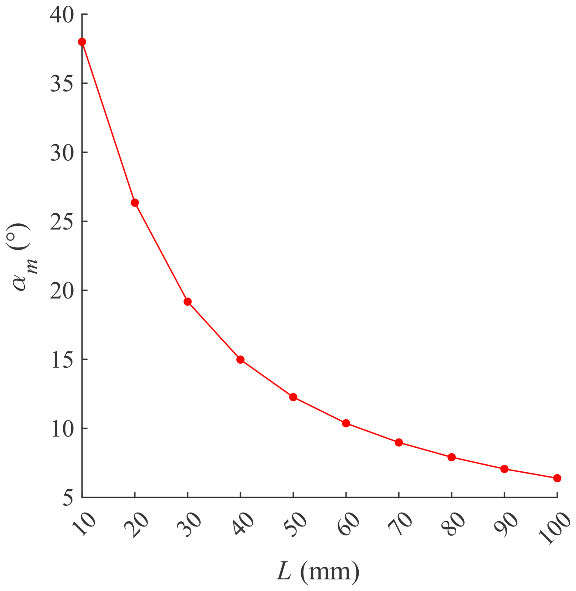
Control the end to move along a given circular trajectory with the center at (0, 0, 250 mm) and a radius r of 80 mm. Keep other physical quantities unchanged (for example, b=16, D=127 mm). Only change the value of the distance L from the center of gravity to the quadrilateral B₁B₂B₃B₄. Analyze the relationship between L and α_m, as shown in Fig. 9.

The larger L is, the smaller α_m is. When L exceeds 70 mm, the deceleration of α_m becomes slow. Appropriately increasing the value of L could make the absolute value of the attitude angle of the robot end as small as possible during the movement. However, this method is not the best strategy to eliminate the attitude angle, as it usually causes the center of gravity distance value L to be very large.

In a fully constrained CDPR, the attitude of the end effector is completely determined by the geometric constraints imposed by the cable length. By combining the equilibrium equations of the force system and the cable length expression and eliminating the tension of the cable, we can obtain the geometric constraint equation that determines the attitude of the end. Therefore, when the cables are all in a tense state, the attitude of the end is independent of the magnitude of the gravity at the end. To iterate the accurate attitude angle, the gravity can be appropriately increased in the iterative Eqs. (1)–(7) to keep the cable in a tense state to avoid iterating inaccurate attitude angles.

When the robot end moves, the cables should be in a tense state and cannot contact the frame. The robot end cannot collide with the frame. Therefore, the geometric constraints that the endpoint E needs to have in the workspace include the following:

1. The projection of the connection point B_i on the plane XOY cannot exceed the boundary of the projection of the quadrilateral A₁A₂A₃A₄ on the plane.

2. The bottom of the robot end cannot collide with the bottom of the frame during movement.

3. The height of the robot end cannot be higher than the quadrilateral A₁A₂A₃A₄.

The geometric constraints of the workspace reachable by point E (relative to the global coordinate system) can be approximated by the following mathematical expression:

$$\begin{array}{}\text{(11)}& \left\{\begin{array}{l}\left|x_E\right|\le D-b\\ \left|y_E\right|\le D-b\\ \mathrm{0}\le z_E\le h\end{array}\right..\end{array}$$

The workspace of the four-cable robot is approximately a cuboid (the area of blue discrete points), with E₃F₃ as the height and quadrilateral F₁F₂F₃F₄ as the bottom (the letter subscripts of the workspace are in the same order as the letter subscripts of the frame), as shown in Fig. 10.

When point E is on the Z axis, it is easy to find that the attitude angle of the robot end is 0. In general, the more the robot end deviates from the Z axis, the larger the attitude angle value tends to be. When moving in a direction other than the X axis, the angle α of the robot end is usually not 0. Therefore, to obtain the maximum value of β, the robot end should be moved close to the center line of the outer side of the frame.

Figure 10 Reachable workspace.

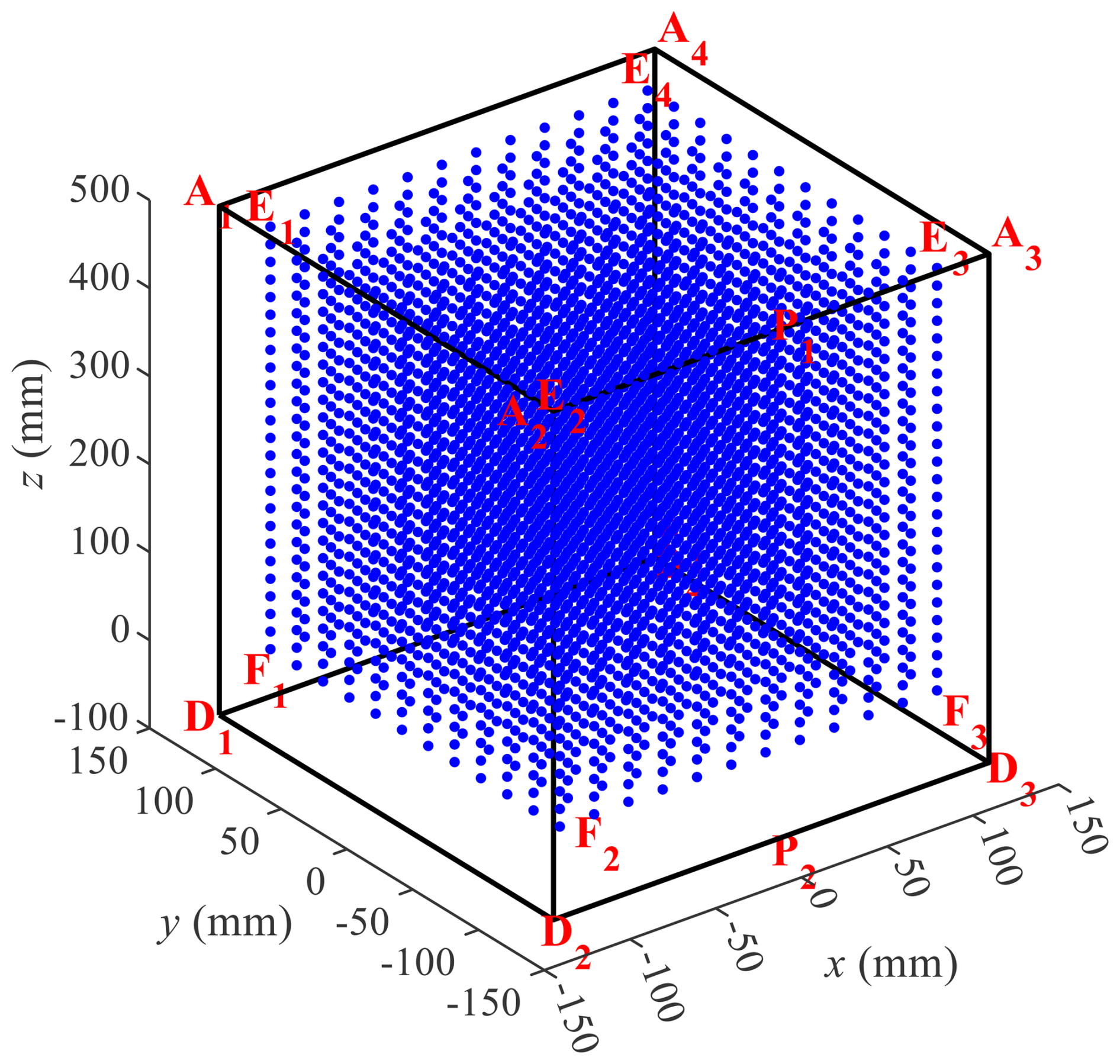
As shown in Fig. 10, assume that the midpoint of A₂A₃ is P₁ and the midpoint of D₂D₃ is P₂. Let the robot end move along the trajectory (12) close to the line segment P₁P₂ to obtain the maximum value of β.

$$\begin{array}{}\text{(12)}& \left\{\begin{array}{l}x=D-b\\ y=\mathrm{0}\\ \mathrm{0}\le z<h\end{array}\right.\end{array}$$

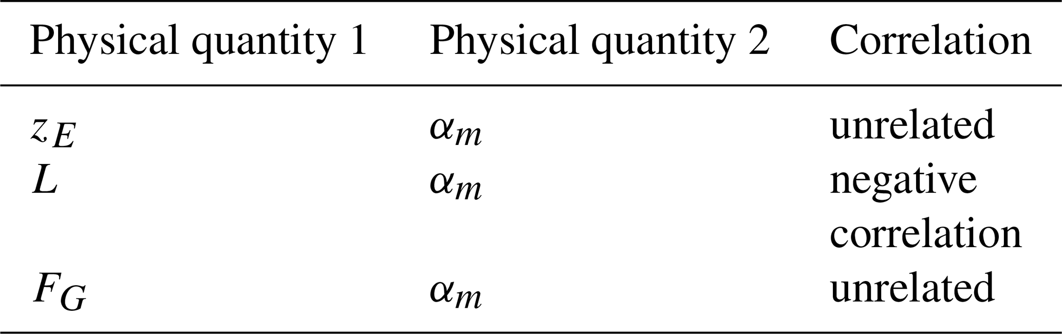
The relationship between the various parameters of the cable robot is shown in Table 1.

Table 1 Comparison of the correlations of the physical quantities.

2.2 Assembly of the kinematic model of the rigid-flexible coupling parallel mechanism

According to the aforementioned rigidification equivalence assumption and the structural characteristics of the cable parallel robot, the chord length and arc length of the elastic thin rod are on the same plane, that is, the elastic thin rod conforms to pure bending and ignores the simplification of small torsion. Therefore, the planar chain beam model and the kinematic model of the four-cable parallel robot can be assembled to derive the kinematic model of the rigid-flexible coupling parallel robot driven by elastic thin rods.

2.2.1 Planar chain beam modeling

The common large deformation analysis model for beams is the chain beam constraint model, which can be used to solve the arc length of the elastic thin rod mentioned above.

Figure 11 Planar-compliant beam.

Figure 12 Geometric relationship of the ith beam.

Figure 13 Structural diagram.

Table 2 Motion trajectory equation.

Figure 14 Iterative method flowchart.

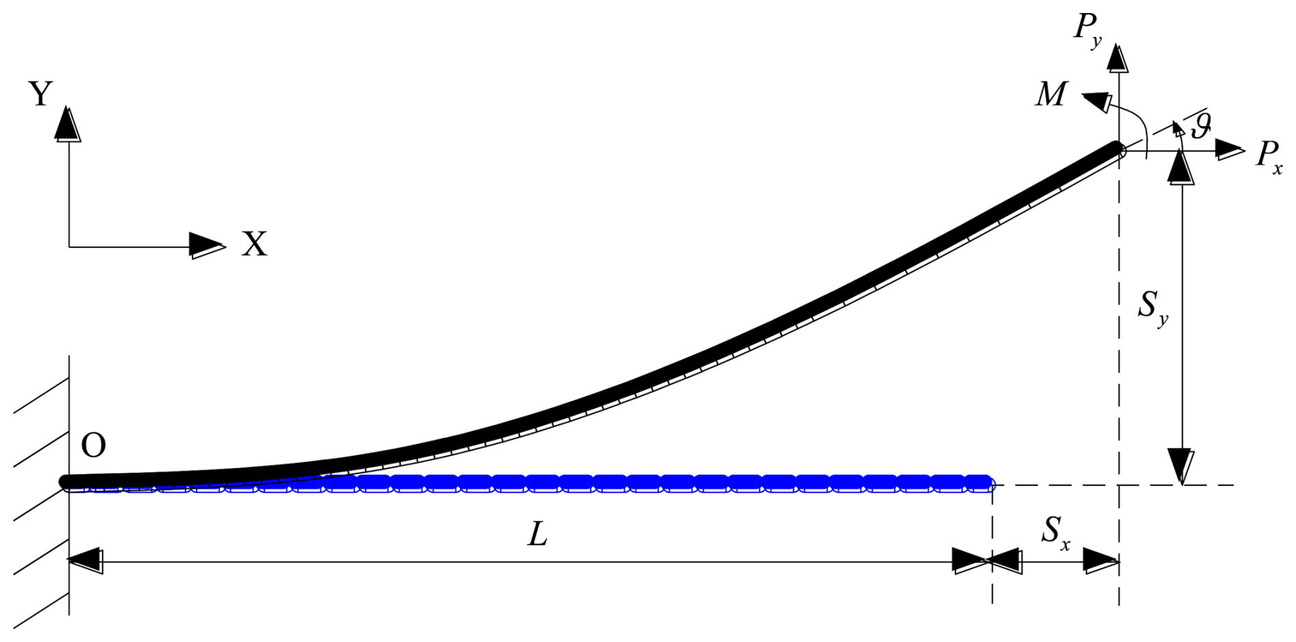
As shown in Fig. 11, assume that one end of the cantilever beam is fixed at point O, the blue segment corresponds to the initial position of the beam without bending deformation, and L is the length of the beam before bending. When a load (including horizontal force P_x, vertical force P_y, and moment M) is applied to the other end, the beam bends and moves to the position of the black arc segment. S_x and S_y are the horizontal displacement and longitudinal displacement of the terminal end relative to the global coordinate system OXY, respectively. ϑ is the angle at the end of the beam. W and T are the out-of-plane thickness and in-plane thickness of the beam section, respectively. Based on the Euler–Bernoulli beam assumption, the cross-section of the beam that was originally flat before deformation remains flat after deformation and is still perpendicular to the axis of the beam after deformation. E is the elastic modulus of the material, and I is the moment of inertia of the section about the Z axis. The constraint equation of the beam is

$$\begin{array}{}\text{(13)}& {\displaystyle }\begin{array}{rl}& \left[\begin{array}{l}{p}_y\\ m\end{array}\right]=\left[\begin{array}{ll}\mathrm{12}& -\mathrm{6}\\ -\mathrm{6}& \mathrm{4}\end{array}\right]\left[\begin{array}{l}{s}_y\\ \mathit{\vartheta }\end{array}\right]+p_x\left[\begin{array}{ll}\mathrm{6}/\mathrm{5}& -\mathrm{1}/\mathrm{10}\\ -\mathrm{1}/\mathrm{10}& \mathrm{2}/\mathrm{15}\end{array}\right]\\ & \left[\begin{array}{l}{s}_y\\ \mathit{\vartheta }\end{array}\right]+p_x^{\mathrm{2}}\left[\begin{array}{ll}-\mathrm{1}/\mathrm{700}& \mathrm{1}/\mathrm{1400}\\ \mathrm{1}/\mathrm{1400}& -\mathrm{11}/\mathrm{6300}\end{array}\right]\left[\begin{array}{l}{s}_y\\ \mathit{\vartheta }\end{array}\right],\end{array}\text{(14)}& {\displaystyle }\begin{array}{rl}& s_x={\displaystyle \frac{t^{\mathrm{2}}{p}_x}{\mathrm{12}}}-{\displaystyle \frac{\mathrm{1}}{\mathrm{2}}}\left[\begin{array}{ll}{s}_y& \mathit{\vartheta }\end{array}\right]\left[\begin{array}{ll}\mathrm{6}/\mathrm{5}& -\mathrm{1}/\mathrm{10}\\ -\mathrm{1}/\mathrm{10}& \mathrm{2}/\mathrm{15}\end{array}\right]\left[\begin{array}{l}{s}_y\\ \mathit{\vartheta }\end{array}\right]\\ & -p_x\left[\begin{array}{ll}{s}_y& \mathit{\vartheta }\end{array}\right]\left[\begin{array}{ll}-\mathrm{1}/\mathrm{700}& \mathrm{1}/\mathrm{1400}\\ \mathrm{1}/\mathrm{1400}& -\mathrm{11}/\mathrm{6300}\end{array}\right]\left[\begin{array}{l}{s}_y\\ \mathit{\vartheta }\end{array}\right].\end{array}\end{array}$$

Inside, $t=T/L$, $p_x=P_x{L}^{\mathrm{2}}/\left(EI\right)$, $p_y=P_y{L}^{\mathrm{2}}/\left(EI\right)$, $m=ML/\left(EI\right)$, $s_x=S_x/L$, and $s_y=S_y/L$. These parameters represent the normalization of the load and displacement variables with respect to the beam parameters.

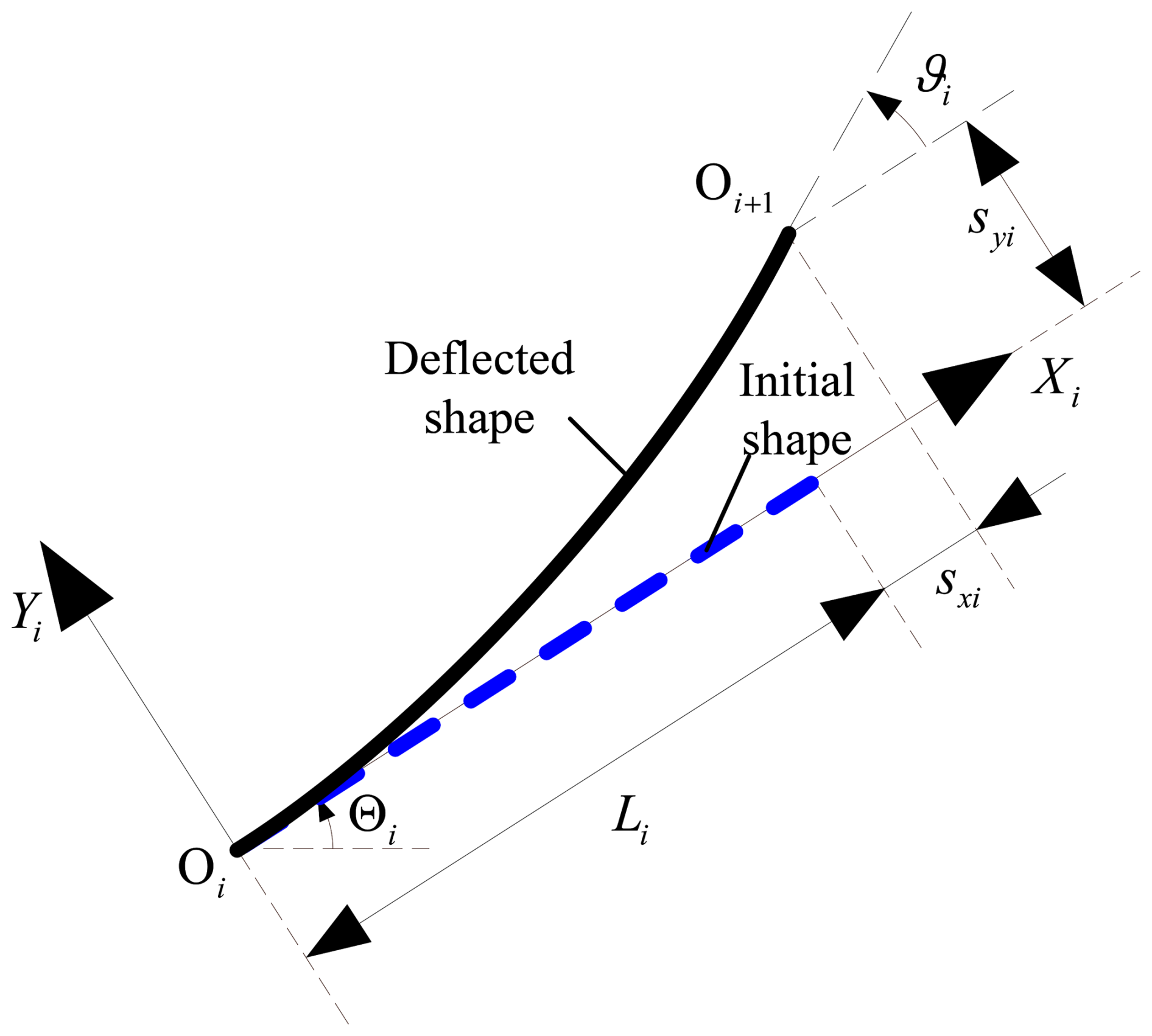
The cantilever beam is divided into N parts, and the length of each unit is $L_i=L/N$. As shown in Fig. 12, for the ith ($\mathrm{1}\le i\le N$) beam unit, in its local coordinate system O_iX_iY_i, it can be regarded as a cantilever at the node O_i, and the free end is the node O_i+1. Equations (13) and (14) are the constraint equations of a single beam unit, and the constraint equations of other beam units can be listed similarly.

Relative to the local coordinate system O_iX_iY_i, assume that the free end of the ith beam element is subjected to the horizontal force P_xi, vertical force P_yi, and moment M_i. According to the force balance, the force balance equation of each beam element is obtained:

$$\begin{array}{}\text{(15)}& \left[\begin{array}{lll}\cos {\mathrm{\Theta }}_i& \sin {\mathrm{\Theta }}_i& \mathrm{0}\\ -\sin {\mathrm{\Theta }}_i& \cos {\mathrm{\Theta }}_i& \mathrm{0}\\ \mathrm{1}+s_{xi}& -s_{yi}& \mathrm{1}\end{array}\right]\left[\begin{array}{l}{p}_{yi}\\ p_{xi}\\ m_i\end{array}\right]=\left[\begin{array}{l}{p}_{y\mathrm{1}}\\ p_{x\mathrm{1}}\\ m_{i-\mathrm{1}}\end{array}\right].\end{array}$$

Inside, $p_{xi}=P_{xi}{L}_i^{\mathrm{2}}/\left(EI\right)$, $p_{yi}=P_{yi}{L}_i^{\mathrm{2}}/\left(EI\right)$, and $m_i=M_i{L}_i/\left(EI\right)$.

The end rotation angle of the ith beam element relative to the global coordinate system OXY is

$$\begin{array}{}\text{(16)}& {\mathrm{\Theta }}_i=\sum _{k=\mathrm{1}}^{i-\mathrm{1}}{\mathit{\vartheta }}_k(i=\mathrm{2},\mathrm{3},\mathrm{\dots },N).\end{array}$$

Assume that the horizontal force on the free end of the elastic thin rod is P_xo, the vertical force is P_yo, the torque is M_o, and the rotation angle is Θ_o. It is easy to find that Θ₁=0; then, we have the following:

$$\begin{array}{}\text{(17)}& \left\{\begin{array}{l}{p}_{x\mathrm{1}}=p_{xo}\\ p_{y\mathrm{1}}=p_{yo}\\ m_N=m_o\end{array}\right..\end{array}$$

Inside, $p_{xo}=P_{xo}{L}_i^{\mathrm{2}}/\left(EI\right)$, $p_{yo}=P_{yo}{L}_i^{\mathrm{2}}/\left(EI\right)$, and $m_o=M_o{L}_i/\left(EI\right)$.

The geometric constraint equations of the beam are

$$\begin{array}{}\text{(18)}& \left\{\begin{array}{l}\sum _{i=\mathrm{1}}^N\left[\right(\mathrm{1}+p_{xi})\cos {\mathrm{\Theta }}_i-p_{yi}\sin {\mathrm{\Theta }}_i]=x_o\\ \sum _{i=\mathrm{1}}^N\left[\right(\mathrm{1}+p_{xi})\sin {\mathrm{\Theta }}_i-p_{yi}\cos {\mathrm{\Theta }}_i]=y_o\\ \sum _{i=\mathrm{1}}^N{\mathit{\vartheta }}_i={\mathrm{\Theta }}_o\end{array}\right..\end{array}$$

Inside, $x_o=X_o/L_i$, and $y_o=Y_o/L_i$.

Through the above analysis, there are a total of (7N+3) equations, including the constraint model equations of 3N beam elements, three (N−1) force system equilibrium equations, three geometric constraint equations, the global rotation expressions of N nodes O_i, and the three equations in equation group (17). Among the six parameters X_o, Y_o, Θ_o, P_xo, P_yo, and M_o, given any three parameters, the other three parameters can be obtained by solving the chain beam model.

2.2.2 Model assembly

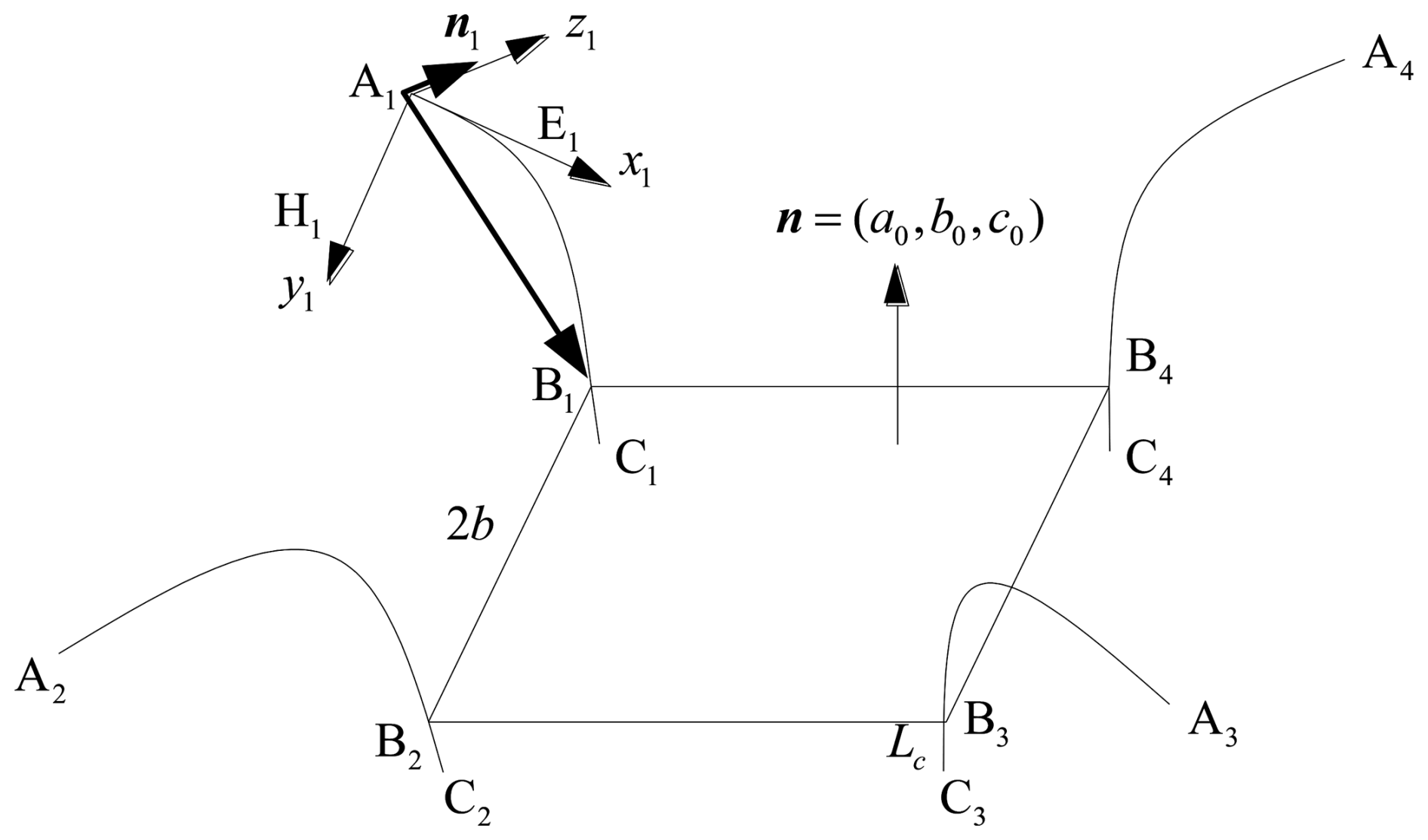
The inverse kinematics model of the rigid-flexible coupling parallel mechanism driven by the elastic thin rods is assembled from the inverse kinematics model of the four-cable robot and the planar chain beam model. The structural diagram of the rigid-flexible coupling parallel mechanism is shown in Fig. 13. Point A_i ($i=\mathrm{1},\mathrm{2},\mathrm{3},\mathrm{4}$) is the fixed point of the flexible thin rod on the frame, point B_i is the point of the flexible thin rod on the end connector of the robot, and C_i is the projection point of B_i on the top surface of the robot. The side length of the top surface B₁B₂B₃B₄ of the end of the robot is 2b, and the direction vector of the external normal of the top surface of the end is set to n. According to the kinematic analysis of the four-cable parallel robot, the spatial coordinates of point B_i and the normal vector n can be regarded as known quantities. Because the slight torsion of the elastic thin rod is ignored, the four flexible thin rods are respectively in four dynamic planes.

Figure 15 Four-cable parallel robot test platform.

Figure 16 Rigid-flexible coupling parallel mechanism test platform.

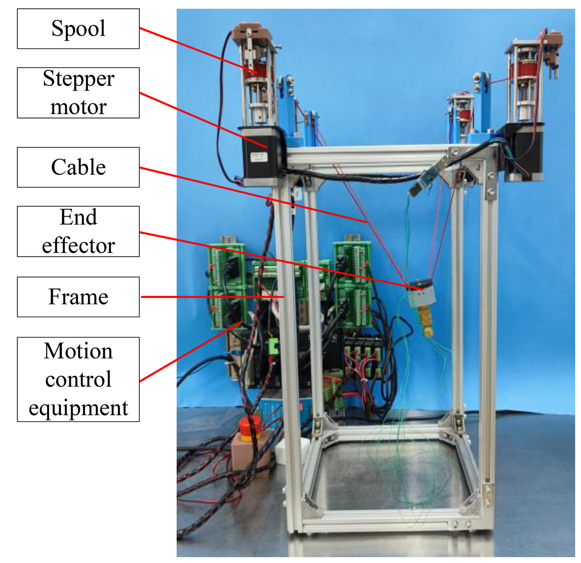
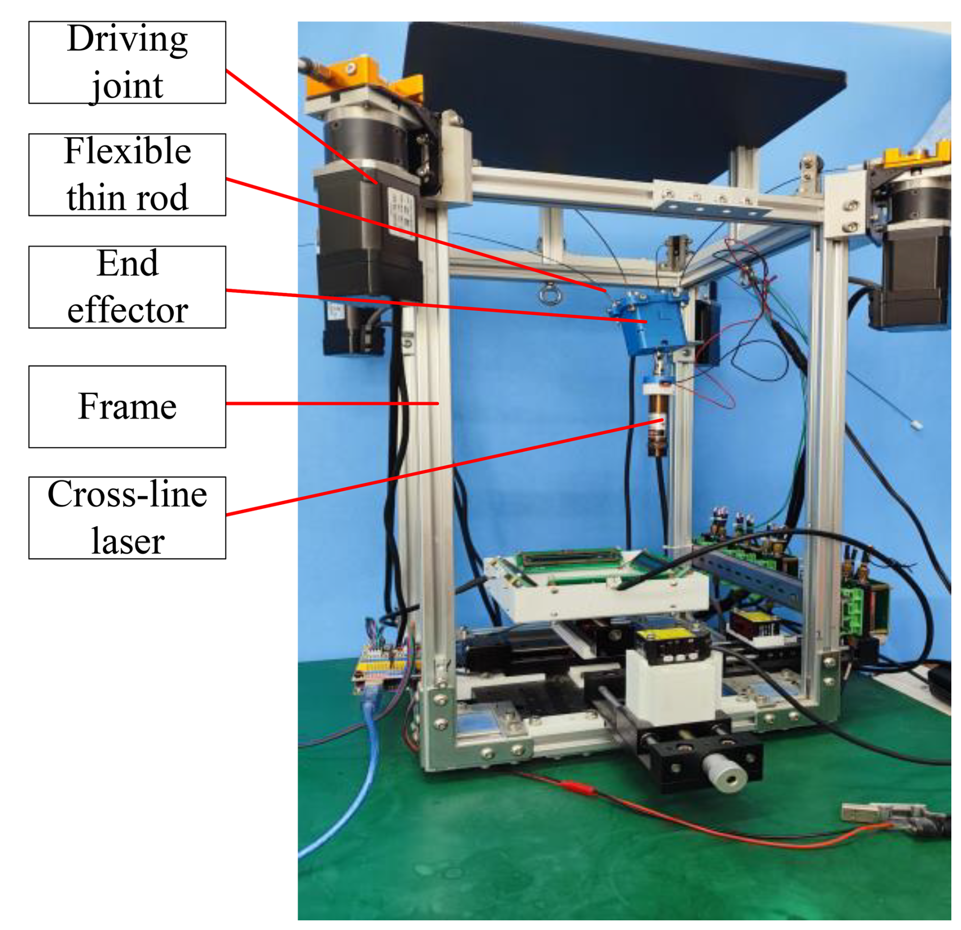
Table 3 Fréchet distance between actual and theoretical curves.

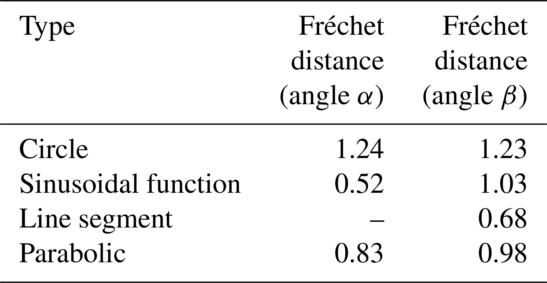
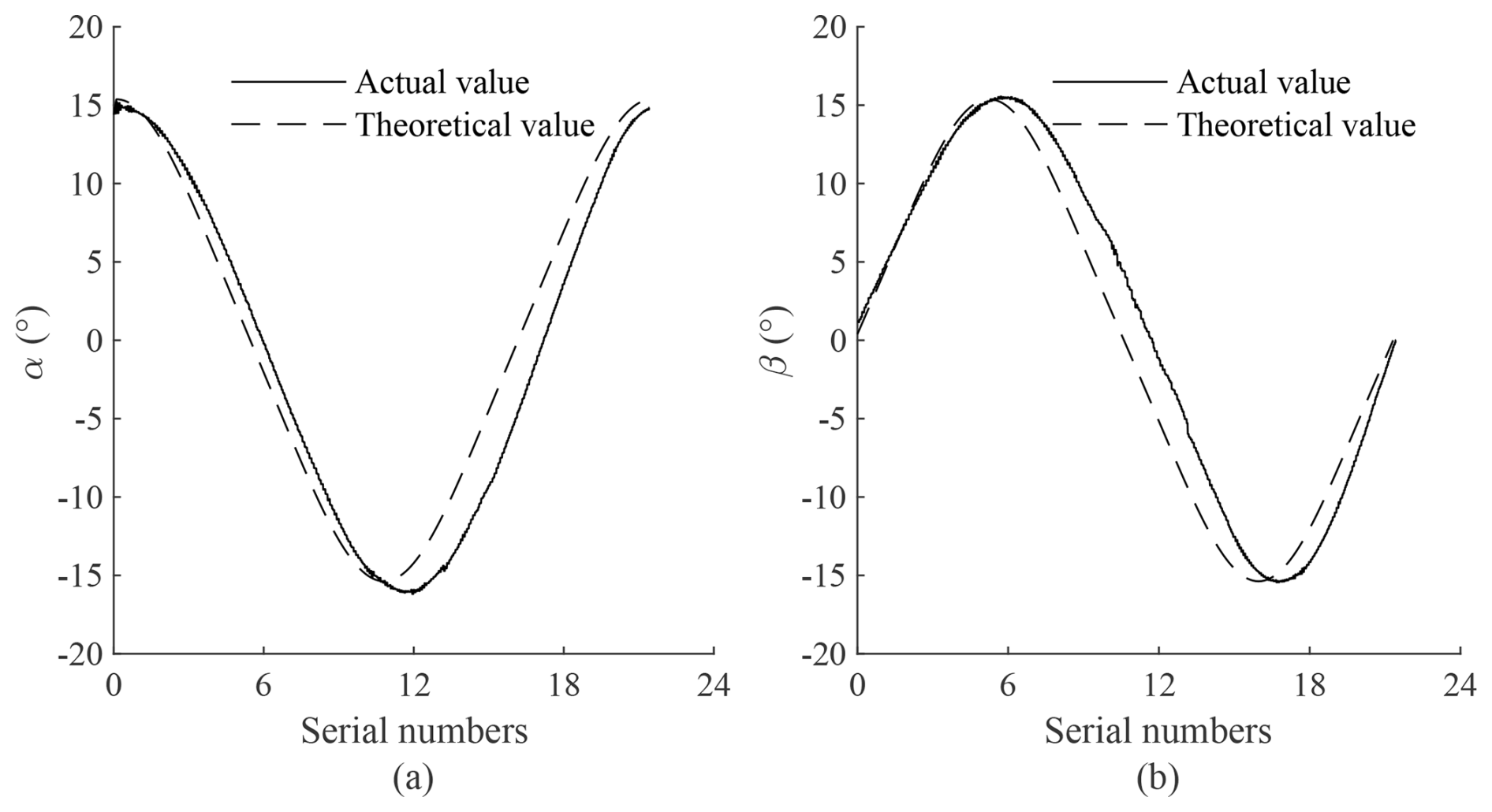
Figure 17 Comparison of attitude angles of the circular trajectory. (a) Comparison of angle α. (b) Comparison of angle β.

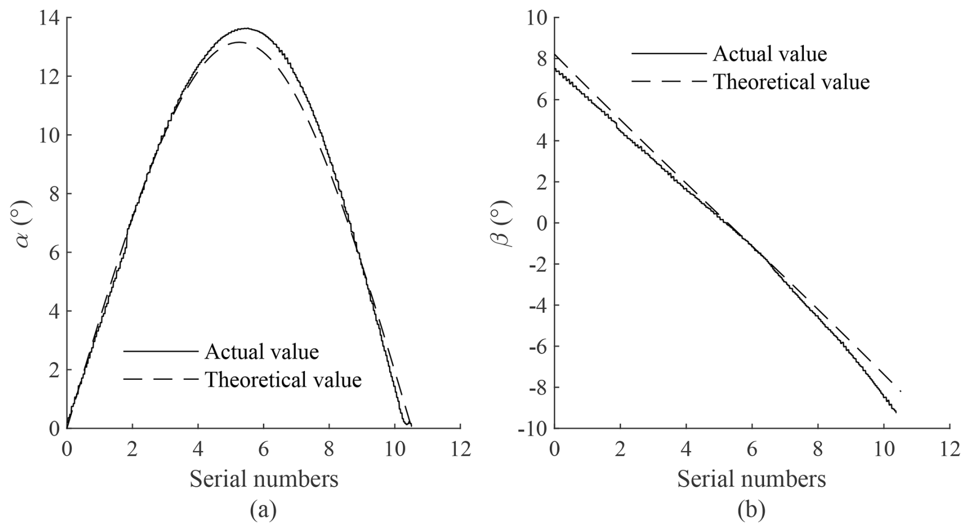
Figure 18 Comparison of attitude angles of the sinusoidal function trajectory. (a) Comparison of angle α. (b) Comparison of angle β.

Figure 19 Angle β comparison of the line segment.

To calculate the arc length of flexible thin rods using the plane chain beam model, it is necessary to know the horizontal and vertical coordinates and the rotation angle of the end of the flexible thin rod in the plane coordinate system where the thin rod is located, as well as the original length of the flexible thin rod before bending. To solve these physical quantities, it is necessary to solve the position of the plane where the flexible thin rod is located. Because the distance between point B_i and point C_i is very short (assuming the distance is L_c) and there is no point with a definite spatial coordinate between the arc segment A_iB_i, point C_i is regarded as a point passing through the plane A_iB_iC_i where the flexible thin rod is located, and we can obtain

$$\begin{array}{}\text{(19)}& \left\{\begin{array}{l}\left|{\mathit{B}}_i{\mathit{C}}_i\right|=L_c\\ {\mathit{B}}_i{\mathit{C}}_i\times (-\mathit{n})=\mathbf{0}\end{array}\right..\end{array}$$

The global coordinates of point C_i can be obtained by using equation group (19). Points A₁, B₁, and C₁ are coplanar. The normal vector n₁ of the surface A₁B₁C₁ can be obtained by using the coordinates of these three points. The global coordinates of A₁ are known to be (−D, D, h). Substitute them into the general equation of the space plane, and the equation of the surface A₁B₁C₁ is

$$\begin{array}{}\text{(20)}& a_{\mathrm{1}}x+b_{\mathrm{1}}y+c_{\mathrm{1}}z+(a_{\mathrm{1}}D-b_{\mathrm{1}}D-c_{\mathrm{1}}h)=\mathrm{0}.\end{array}$$

Draw the x₁ axis through point A₁ and make it tangent to the thin rod at point A₁. Because the extended end of the beam at the starting point A₁ is horizontal, the x₁ axis is located in the plane A₁A₂A₃A₄. By combining plane A₁B₁C₁ and plane A₁A₂A₃A₄, we can get the equation of the space line where the x₁ axis is located:

$$\begin{array}{}\text{(21)}& \left\{\begin{array}{l}{a}_{\mathrm{1}}x+b_{\mathrm{1}}y+c_{\mathrm{1}}z+(a_{\mathrm{1}}D-b_{\mathrm{1}}D-c_{\mathrm{1}}h)=\mathrm{0}\\ z=h\end{array}\right..\end{array}$$

Take any point E₁ on the positive direction of the x₁ axis. The spatial coordinates of point E₁ are known, and it is easy to find that A₁E₁ is the direction vector of the x₁ axis. Draw the z₁ axis through point A₁ perpendicular to the surface A₁B₁C₁, and the direction vector of the z₁ axis is n₁. In the local coordinate system A₁-x₁y₁z₁, the direction vector of the y₁ axis is

$$\begin{array}{}\text{(22)}& {\mathit{A}}_{\mathrm{1}}{\mathit{H}}_{\mathrm{1}}={\mathit{n}}_{\mathrm{1}}\times {\mathit{A}}_{\mathrm{1}}{\mathit{E}}_{\mathrm{1}}.\end{array}$$

Inside, H₁ is a point on the y₁ axis.

The projection length of A₁B₁ on the x₁ axis is

$$\begin{array}{}\text{(23)}& x_{o\mathrm{1}}={\displaystyle \frac{{\mathit{A}}_{\mathrm{1}}{\mathit{B}}_{\mathrm{1}}\cdot {\mathit{A}}_{\mathrm{1}}{\mathit{E}}_{\mathrm{1}}}{\left|{\mathit{A}}_{\mathrm{1}}{\mathit{E}}_{\mathrm{1}}\right|}}.\end{array}$$

The projection length of A₁B₁ on the y₁ axis is

$$\begin{array}{}\text{(24)}& y_{o\mathrm{1}}={\displaystyle \frac{{\mathit{A}}_{\mathrm{1}}{\mathit{B}}_{\mathrm{1}}\cdot {\mathit{A}}_{\mathrm{1}}{\mathit{H}}_{\mathrm{1}}}{\left|{\mathit{A}}_{\mathrm{1}}{\mathit{H}}_{\mathrm{1}}\right|}}.\end{array}$$

(x_o1, y_o1) is the coordinate of point B₁ in the plane coordinate system x₁A₁y₁. The rotation angle of the elastic thin rod at point B₁ is approximately equal to the angle θ₁ between B₁C₁ and A₁E₁, which is an acute angle. Its expression is

$$\begin{array}{}\text{(25)}& {\mathit{\theta }}_{\mathrm{1}}\approx \arccos {\displaystyle \frac{{\mathit{B}}_{\mathrm{1}}{\mathit{C}}_{\mathrm{1}}\cdot {\mathit{A}}_{\mathrm{1}}{\mathit{E}}_{\mathrm{1}}}{\left|{\mathit{B}}_{\mathrm{1}}{\mathit{C}}_{\mathrm{1}}\right|\cdot \left|{\mathit{A}}_{\mathrm{1}}{\mathit{E}}_{\mathrm{1}}\right|}}.\end{array}$$

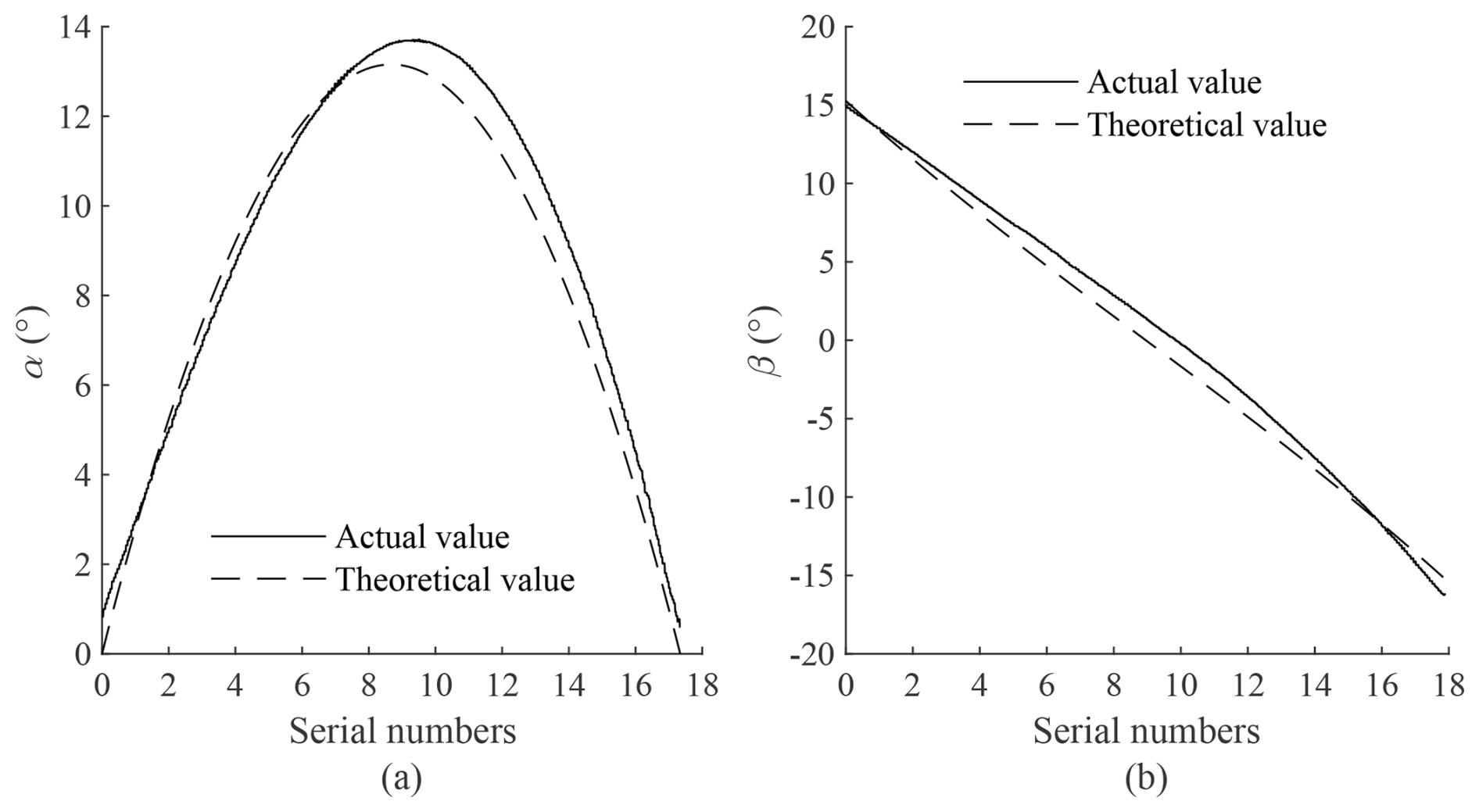
Figure 20 Parabolic trajectory attitude angle comparison. (a) Comparison of angle α. (b) Comparison of angle β.

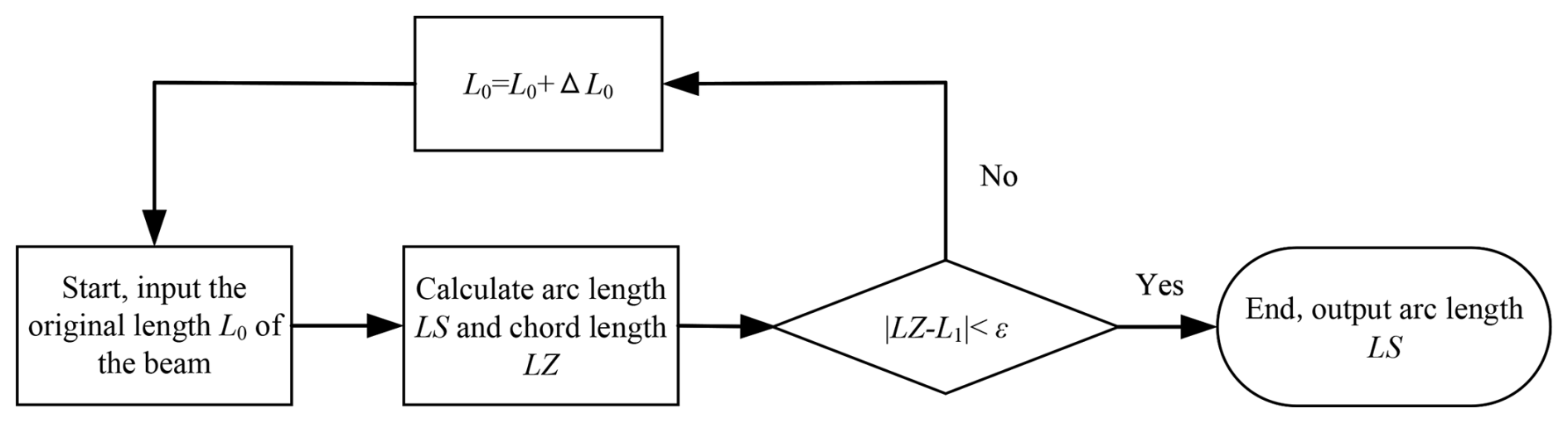
Because the length of the elastic thin rod before bending is always changing, this paper adopts the iterative method to solve the problem. The flowchart of the iterative method is shown in Fig. 14. The solution process of the iterative method is described as follows:

1. Set the initial length of the thin rod L₀.

2. According to the existing conditions, the chain beam model is used to solve the arc length LS and chord length LZ of the thin rod after bending.

3. Calculate the difference between the chord length LZ and the cable length L₁ in the equivalent model.

4. If $\left|LZ-L_{\mathrm{1}}\right|>\mathit{\epsilon }$, then add an increment to the original L₀ and return 1; if $\left|LZ-L_{\mathrm{1}}\right|\le \mathit{\epsilon }$, then the arc length LS is the physical quantity to be solved.

3 Results and discussions

To verify the accuracy of the kinematic model of the four-cable robot, a motion control test platform was built, as shown in Fig. 15. The test platform consists of four spools, four stepper motors, four cables, an end effector, a frame, and motion control equipment. The model number of the stepper motor is 42HB250-60B, and the motion control equipment uses the Galil DMC-4143.

After completing the motion control test of the four-cable robot, the end of the four-cable robot is replaced, and its driving component (thin cable) is replaced with an elastic thin rod, thus obtaining a rigid-flexible coupling parallel mechanism driven by elastic thin rods. To verify the accuracy of the inverse kinematic model of the rigid-flexible coupling parallel mechanism, it is necessary to conduct a motion control test on the mechanism. Its motion control test platform (as shown in Fig. 16) consists of four driving joints (stepper motor), four flexible thin rods, an end effector, a frame, a cross-line laser, and other parts. To achieve real-time measurement feedback of the robot end position with multiple degrees of freedom, a planar three-degree-of-freedom non-contact measurement system is established by integrating a one-dimensional optical position sensor (position sensitive detector, PSD) (Mo et al., 2024), as shown in Fig. 16. The model number of the one-dimensional PSD sensor is DRX-1DPSD-0A03-70. The cross-line laser emitted by the cross-line laser will be sensed by four one-dimensional PSDs, resulting in four light spots. The model number of the cross-line laser is the CMOS type HG-C1200, which is from Panasonic. The planar three degrees of freedom of the end are calculated based on the position of the light spots. The specific results and principles of the measurement system can be found in the literature (Mo et al., 2024; Wen et al., 2025).

3.1 Test results of the four-cable robot

The endpoint E of the four-cable robot is controlled to move along the trajectory $x^{\mathrm{2}}+y^{\mathrm{2}}={\mathrm{80}}^{\mathrm{2}}(z=\mathrm{200})$. The unit is millimeters. The rotation angle of the end during the movement is measured by the gyroscope and then compared with the theoretical value, as shown in Fig. 17. The trajectory similarity between two curves is often evaluated by the Fréchet distance. The smaller the Fréchet distance, the closer the two curves are.

The number of points in the two discrete point sequences is not equal. In order to compare the trajectory similarity between the two curves, the beginning and the end of the two unequal discrete point sequences are overlapped. Therefore, the horizontal coordinate of the discrete points in Fig. 17 is the result of the proportional transformation of the serial numbers of the 200 discrete points. It is a dimensionless value without physical meaning. If the horizontal axis of the graph involving the attitude angle in the following text is marked with “Serial numbers”, the meaning is the same. The hysteresis of signal processing, the hysteresis of force transmission, and the vibration of the end are all factors that cause the increase in the Fréchet distance.

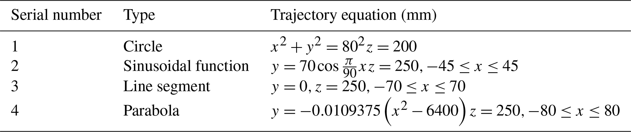
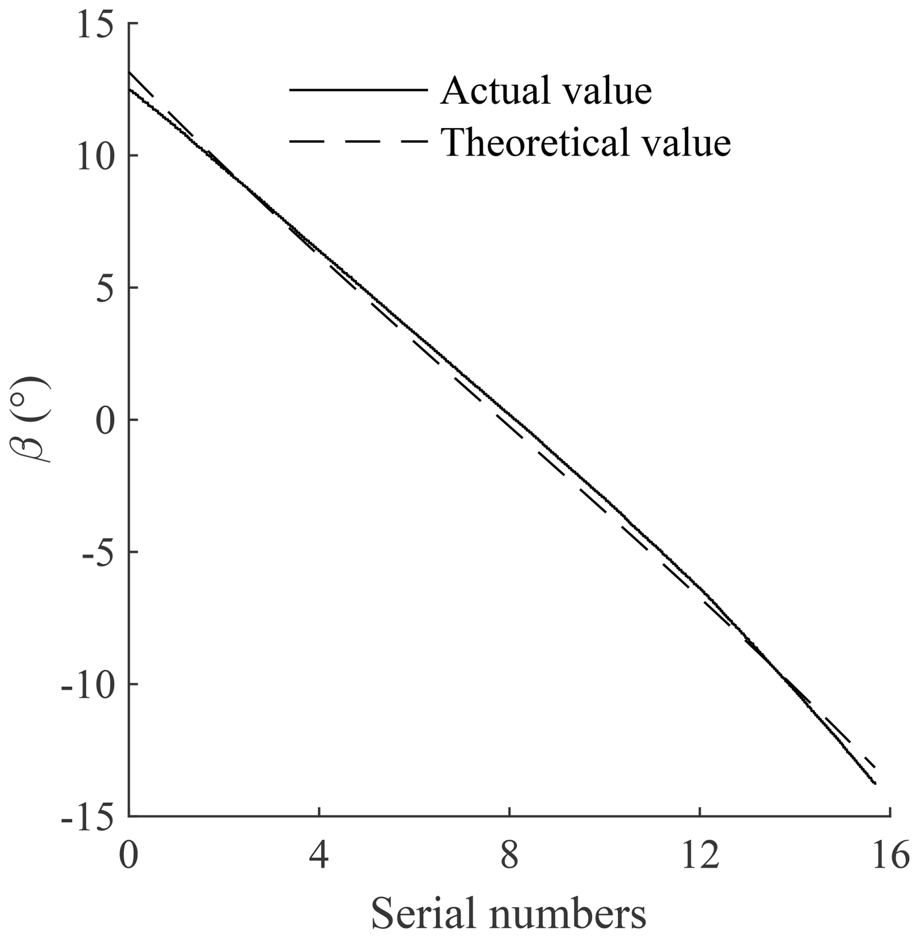
Control point E to move along other trajectories in Table 2, and analyze the kinematics of the robot end. The results are shown in Figs. 18, 19, and 20.

When the robot endpoint E moves along the sinusoidal function trajectory, the value of angle β shows a linear downward trend.

The robot endpoint E has only a displacement component in the X-axis direction in the line segment, and the corresponding angle α is very small and can be ignored.

On the whole, when the robot terminal moves along different trajectories, the actual value and theoretical value of the attitude angle are relatively close.

In Table 3, because the corresponding angle α is very small (essentially 0) when the end moves along the line segment trajectory, the comparison of the Fréchet distance is not very meaningful and is not included in Table 3.

Control point E to move along trajectory (12), that is, move close to line segment P₁P₂ (point E is on the outer side surface E₂F₂F₃E₃ of the workspace), and solve the changing pattern of β, which is shown in Fig. 21. Trajectory (12) is close to the boundary of the workspace, and the end is easily subjected to vibration shock during movement. In order to more accurately measure the change in the end attitude angle, a certain number of discrete position points are taken in trajectory (12). Let the robot end stop at these position points in turn, and record the value of each measured angle β.

Figure 21 The changing pattern of β corresponding to trajectory (12).

When the vertical coordinate z_E of point E exceeds 400 mm, the end of the robot is likely to contact the aluminum profile supporting the bearing bracket, which will cause the attitude angle measured by the gyroscope to be inaccurate. Therefore, the actual value curve in Fig. 21 only has a section where z_E does not exceed 400 mm. Within the range where z_E does not exceed 400 mm, changing the height of point E basically does not affect the amplitude of β, and the error of β is between 1 and 2°. From a theoretical point of view, when point E is very close to the boundary of the top of the workspace, the value of β will change sharply to near 0. The maximum absolute value of β is about 22.5°. The four-cable robot has a high degree of symmetry; therefore, the angle values of α and β are both between −22.5 and 22.5°.

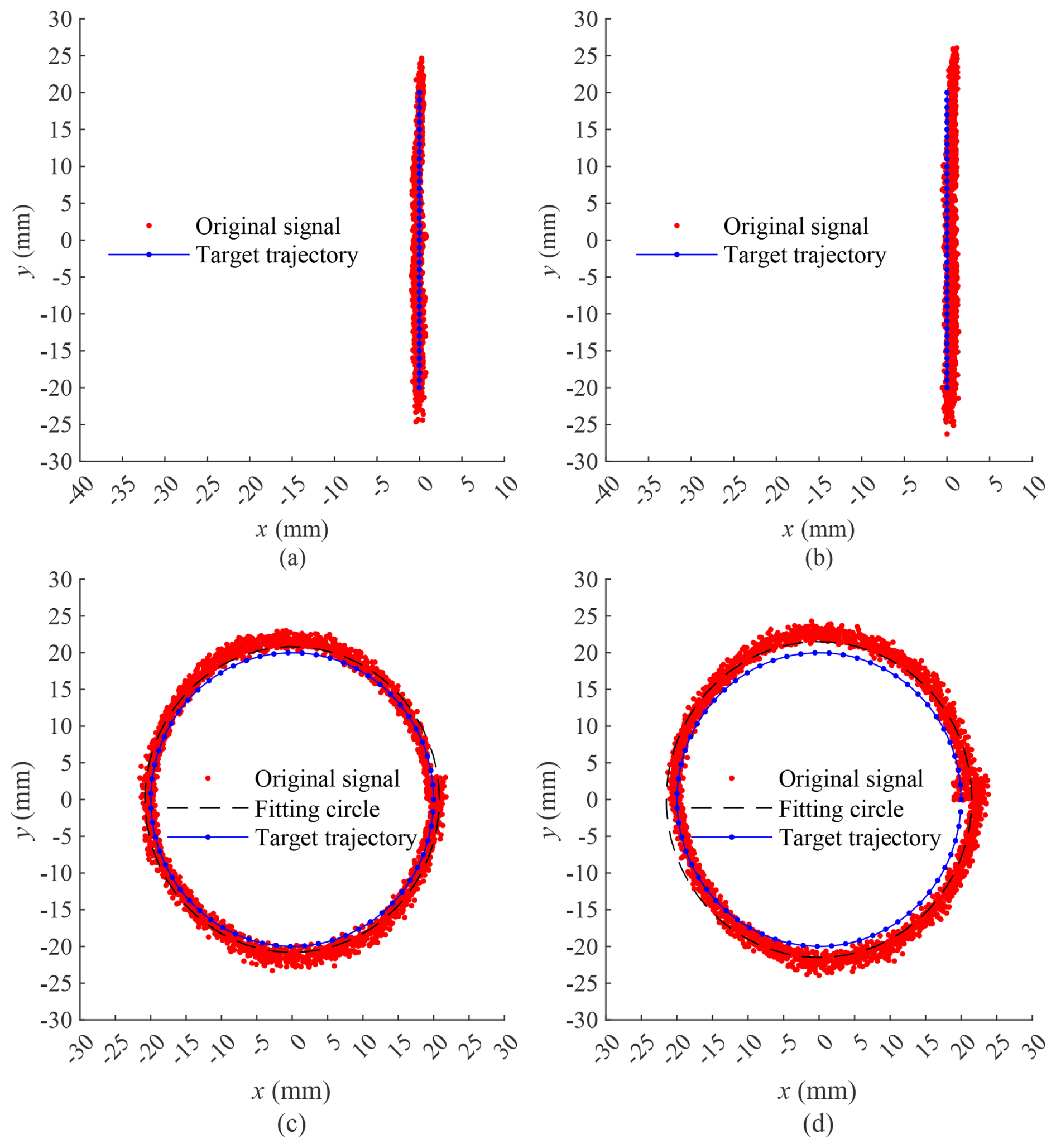
Figure 22 Comparison of target trajectory and original signal. (a) Comparison chart of trajectory (1). (b) Comparison chart of trajectory (2). (c) Comparison chart of trajectory (3). (d) Comparison chart of trajectory (4).

Table 4 Motion trajectory equation.

Looking at the previous motion control experiments, the curves corresponding to the actual values and theoretical values of the attitude angles under different trajectories are very close, proving that the kinematic model of the four-cable parallel robot is accurate.

3.2 Test results of the rigid-flexible coupling parallel mechanism

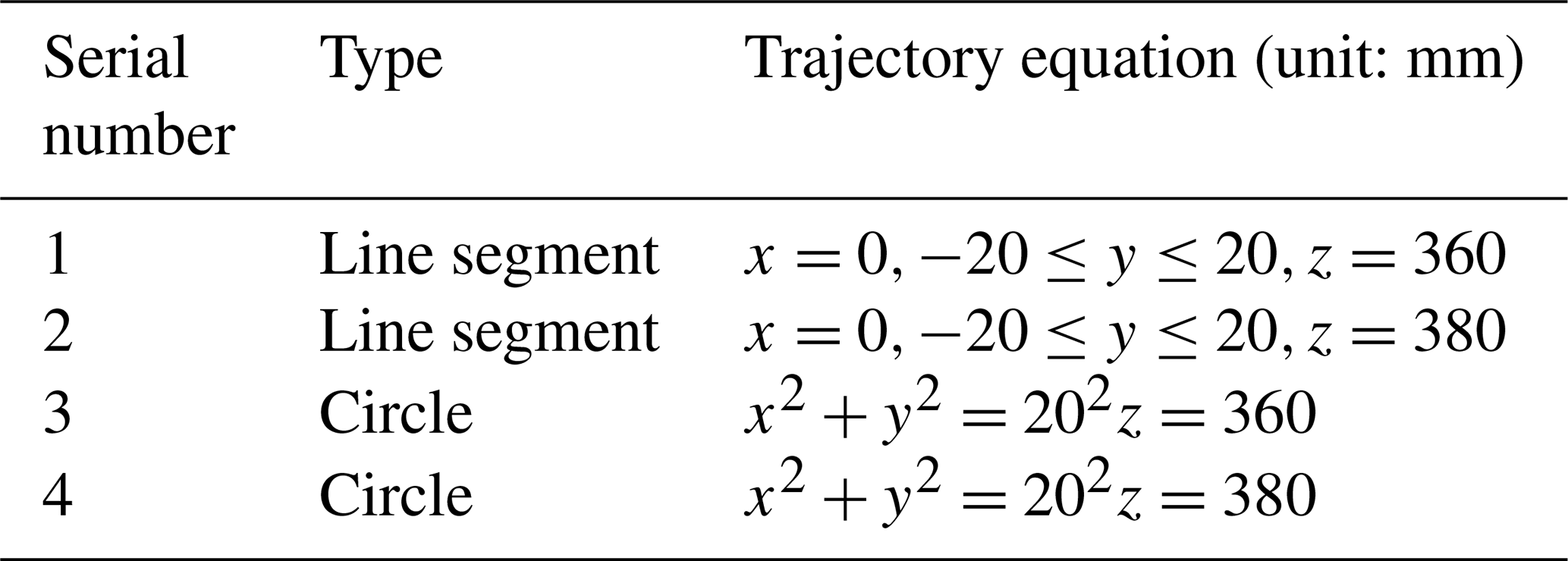
The endpoint E of the rigid-flexible coupling parallel mechanism is controlled to start from the midpoint of the trajectory in Table 4 and move along the trajectory. The error between the target trajectory and the original signal is compared, as shown in Fig. 22. Trajectories (1), (2), (3), and (4) correspond to (a), (b), (c), and (d) in Fig. 22, respectively. The maximum errors between the target trajectory and the original signal in the x-axis direction in Fig. 22a and b are 0.7 and 1.3 mm, respectively, and the error in the y-axis direction can be corrected. The radial errors between the signal fitting circle (fitting the original signal into a circle) and the target trajectory in Fig. 22c and d are 0.8 and 1.5 mm, respectively. In the different trajectories of Fig. 22, the target trajectory and the original signal are relatively close, proving that the kinematic model of the rigid-flexible coupling parallel mechanism driven by elastic thin rods has a certain accuracy within a small range. During the movement of the robot end, there is a phenomenon of vibration of the elastic thin rod, which shows that the limitations of the kinematic model can increase the error between the original signal and the target trajectory. In addition, the closer the starting position is to the midpoint of the line segment, the higher the motion accuracy, and the large deformation degree of the elastic thin rod will affect the motion accuracy of the robot end.

4 Conclusions

This paper mainly conducts a systematic study on the kinematics of the rigid-flexible coupling parallel mechanism driven by elastic thin rods and analyzes and studies the challenges of the inverse kinematics of the rigid-flexible coupling parallel mechanism driven by elastic thin rods. The key innovation points of this paper are as follows:

1. A method of rigidification equivalence is proposed to rigidify the rigid-flexible coupling parallel mechanism driven by elastic thin rods into a four-cable parallel robot.

2. The numerical iteration method is used to solve the kinematic-static coupling problem of the fully constrained cable parallel robot, providing the coordinate information of the connection point between the elastic thin rod and the end of the mechanism for the subsequent study of the inverse kinematics of the rigid-flexible coupling parallel mechanism driven by elastic thin rods. The four-cable suspended parallel robot motion test platform is built to test and verify that the algorithm in this paper has high accuracy.

3. Aiming at the inverse kinematics problem of the rigid-flexible coupling parallel mechanism driven by elastic thin rods, a scheme combining a planar chain beam model and a four-cable parallel robot kinematic model is proposed. First, the two models are assembled to calculate the arc length of the elastic thin rod; then, the motion control test of the rigid-flexible coupling parallel mechanism is carried out, and the error between the theoretical trajectory and the actual trajectory obtained by inverse kinematics is compared, which verifies that the scheme has a certain accuracy in a small range.

This paper has achieved preliminary results in the study of the kinematics of the rigid-flexible coupling parallel mechanism driven by elastic thin rods, but there is still room for improvement in the method design and experimental verification stage. Through further thinking about the kinematics of the rigid-flexible coupling parallel mechanism and combining the relevant problems encountered in this study, the following prospects for this study are proposed:

1. In the motion control experiment of the rigid-flexible coupling parallel mechanism driven by elastic thin rods, although the planar chain beam model is accurate, the precise original beam length and end deflection must be given to iterate the results. The original beam length before bending is unknown and can only be estimated or iterated in advance, which directly affects the accuracy and efficiency of the solution. The estimated value of the original beam length can be changed later to study its impact on the accuracy and efficiency of the solution.

2. In terms of the end measurement of the rigid-flexible coupling parallel mechanism, only the three planar degrees of freedom (the movement degrees of freedom of the X and Y axes and the rotation degrees of freedom around the Z axis) are measured at the end of the mechanism, and the other three degrees of freedom have not been measured. This is because there is no suitable measurement method. A new measurement system needs to be designed in the future to achieve full-degree-of-freedom measurement of the end.

3. There is elastic vibration in the movement process of the rigid-flexible coupling parallel mechanism. Subsequently, by studying its vibration characteristics, we can design a suitable vibration suppression algorithm to improve the controllability, speed, and accuracy of the mechanism's movement.