Cyclostationary analysis of vibration signals from electric motor – understanding of bi-frequency map

Cyclostationary analysis is one of the most promising and powerful methods for analyzing vibration signals from rolling element bearings (REBs). Damage to the REB is one of the most common reasons for failure in the electric motor (EM). Thus, the application of cyclostationary analysis to vibration signals from EM is reasonable in order to detect faults. Unfortunately, it has been observed that analyzing vibration signals measured on bearings in electric motors is much more challenging due to the presence of additional cyclic components on the bi-frequency map that affect the analysis. These additional components may have various mechanical sources (for example, the influence of shaft misalignment) or electrical/electromagnetic origins (such as frequencies related to features of the power source, i.e., grid frequency, inverter keying, etc.). This paper is an introduction to bearing diagnostics in electric motors based on cyclostationary analysis in the bi-frequency domain. We present various cases to show the complexity of the map and conclude that there is a need to define a method for automatic identification and interpretation of sources, i.e., understanding of the bi-frequency map. As other cyclic sources are wideband and they have much stronger values on the map, simple band selection is difficult. Thus, new methods for further map processing and novel indicators to assess the significance of features that describe the fault based on cyclic spectral coherence (CSC) maps should be developed. However, it is stated that it requires a deep understanding of the CSC map. We believe that this paper brings some new knowledge to the context of using CSC for bearing diagnosis in electric motors.

1 Introduction

Condition monitoring of electric motors is an important field of study. There are many techniques to detect failures in electric motors. The classical one is vibration analysis; however, it allows for the detection of mostly mechanical problems in electric motors. Thus, other sources of information have also been investigated (current, speed, torque, sound, temperature, including infrared thermography, image; see more in several review papers (Nandi et al., 2005; Bellini et al., 2008; Vaniya and Chudasama, 2023; Halder et al., 2022)). As rolling element bearing failures are the most common mechanical reason for electric motor breakdown (Nandi et al., 2005), accounting for nearly 40 % of all failure causes, this paper focuses on vibration analysis for bearing fault detection. The most popular method for bearing fault detection is envelope analysis (Randall and Antoni, 2011). However, it often requires some preprocessing, i.e., prefiltering, to extract the signal with a monocomponent carrier before demodulation. Another reason for pre-filtering is related to signal-to-noise ratio improvement. There are many works related to the selection of informative frequency bands; one of the most popular is spectral kurtosis (Antoni and Randall, 2006). Many possible statistics could be used for band selection (Obuchowski et al., 2014), a recent review of existing methods can be found in Hebda-Sobkowicz et al. (2020a). It is also recommended to study the work of Leite et al. (2015), where the authors considered a method for localized bearing fault detection based on the application of spectral kurtosis and envelope analysis applied to the stator current.

Figure 1 Concept of cyclostationary analysis.

Figure 2 Possible scenarios for diagnostic process using bi-frequency map.

1.1 Cyclostationary analysis

Searching for impulsiveness in the time domain or periodic structure in the envelope spectrum are two main directions for bearing diagnostics. However, it has been found that signals from faulty bearings can be considered a special class of nonstationary signals with some cyclic variation in signal properties. Antoni et al. (2004) proposed a framework for cyclostationary modeling for vibration signals. Cyclostationary methods are well-known in other fields, such as telecommunications and oceanography, and can be successfully applied to condition monitoring. It is recommended to read the recent book on trends and applications in cyclostationary analysis of Napolitano (2016). Randall et al. (2001) showed that integrated cyclic spectral correlation integrated over all carrier frequency bins is equal to the amplitude spectrum of the squared envelope of the signal. Raad et al. (2008) proposed indicators of cyclostationary behavior that could be used for condition monitoring. Further work by Antoni (2009) highlighted the practical benefits of using a cyclostationary approach for bearing diagnostics.

It was observed in the literature that cyclostationary analysis is not so popular for bearing diagnostics in induction motors, which is counterintuitive. There are just a few works related to cyclostationarity and electric motors. Even review articles focused on induction motor diagnostics do not consider the cyclostationary properties of vibrations.

In their review, Tandon et al. (2007) discussed vibration velocity and its spectrum, acoustic emission, shock pulse method, and current monitoring. Mauricio et al. (2018) found that bearings diagnostics of electric drives might be hard when motors are controlled by variable-frequency drives. Due to electromagnetic interference (EMI), classic methods may provide rather poor diagnostic performance. They claim that the mentioned disturbances may provide a pattern similar to that of a faulty bearing, making it difficult to detect the true signature of the damage. To overcome the problem, they used two novel diagnostic methodologies based on cyclic spectral coherence (CSC). These methodologies allow for the automatic selection and integration of optimal bands in the CSC. The integration of CSC, over the full spectral frequency axis or a specific spectral frequency band, results in the enhanced or improved envelope spectrum, respectively. The issue of variable-frequency drives has also been raised by Seshadrinath et al. (2014). They conducted an investigation of vibration signatures for multiple fault diagnosis in variable-frequency drives using complex wavelets. Islam and Kim (2018) proposed a procedure for motor bearing fault diagnosis that is based on deep convolutional neural networks with 2D analysis of the vibration signal. Frosini and Bassi (2010) proposed using the stator current and the efficiency of the induction motors as indicators of rolling bearing faults. Minervini et al. (2020) proposed a method based on multisensor measurements to detect cyclic faults in induction motors. However, features have been extracted from the spectral domain at a low-frequency range that requires strong energy components related to the fault. Importantly, Minervini also raised the problem of electromagnetic disturbances.

1.2 Applications of cyclostationary analysis to electric motors

One of the greatest examples of cyclostationarity in bearing diagnosis is a paper provided by Teng et al. (2017). The authors considered a wind turbine generator. They demonstrated that an intrinsic electromagnetic vibration, originating from an alternating magnetic field acting on a low-stiffness stator, modulates the vibration signals of the generator. Consequently, true fault features related to damaged bearings are masked by other cyclic sources. Recently, Wang et al. (2023) proposed a method based on an enhanced cyclostationary approach and its application to the incipient fault diagnosis of induction motors. However, the proposed method is multistage and covers advanced wavelet-based preprocessing and Teager–Kaiser demodulation. Wang et al. (2022) improved the TKEO-based cyclostationary analysis method and its application to the diagnosis of induction motor faults. Another interesting application of cyclostationarity is provided by Wang et al. (2019) in the context of identifying broken rotor bar faults. He et al. (2023) proposed an improved cyclostationary analysis algorithm and its implementation into an edge computing system to diagnose a motor fault in real time. The main focus of that paper was real-time detection. Wang et al. (2020) proposed a combination of decomposition and cyclostationary analysis. It contains genetic mutation particle swarm optimization (GMPSO) with cyclic information entropy (CIE) to optimize the variational mode decomposition parameters; then, a multidomain extreme learning machine has been applied for state recognition. In almost all the mentioned techniques, the authors did not present a bi-frequency map as input data that were used for feature extraction and simple decision-making, or the presented maps, were easy to interpret (no detailed interpretation was provided).

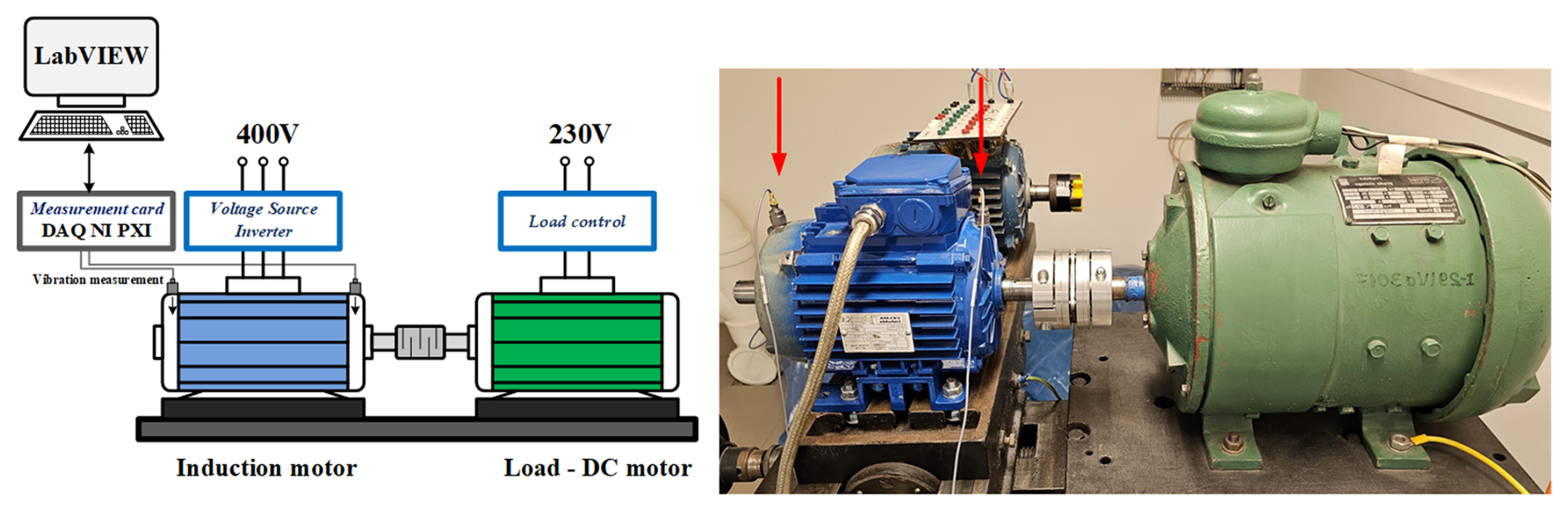
Figure 3 The scheme (left panel) and the photo (right panel) of the test rig. Arrows indicate sensor placement.

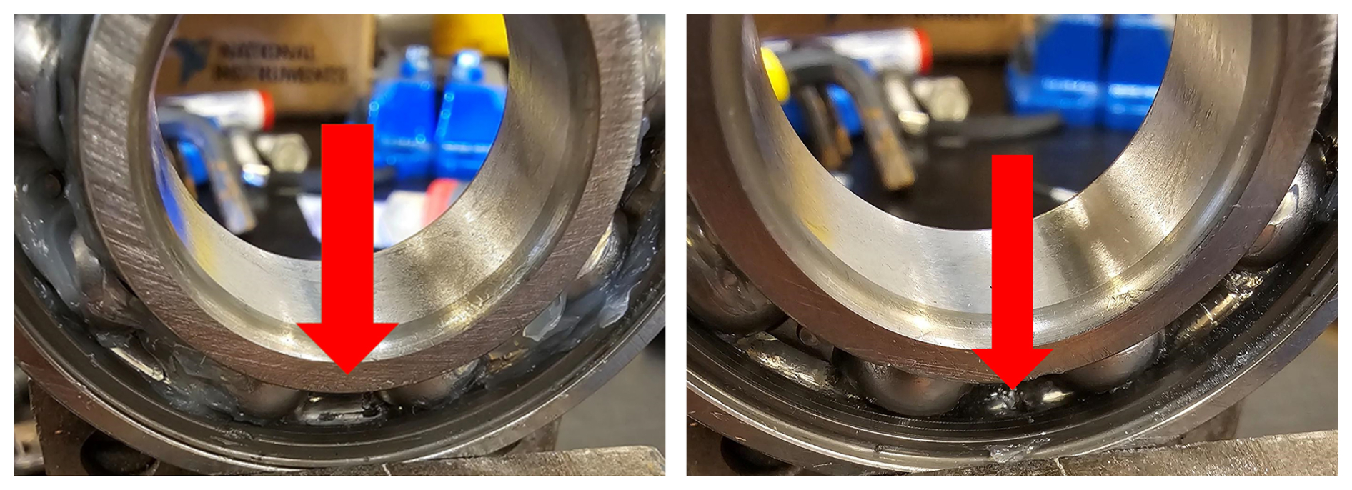
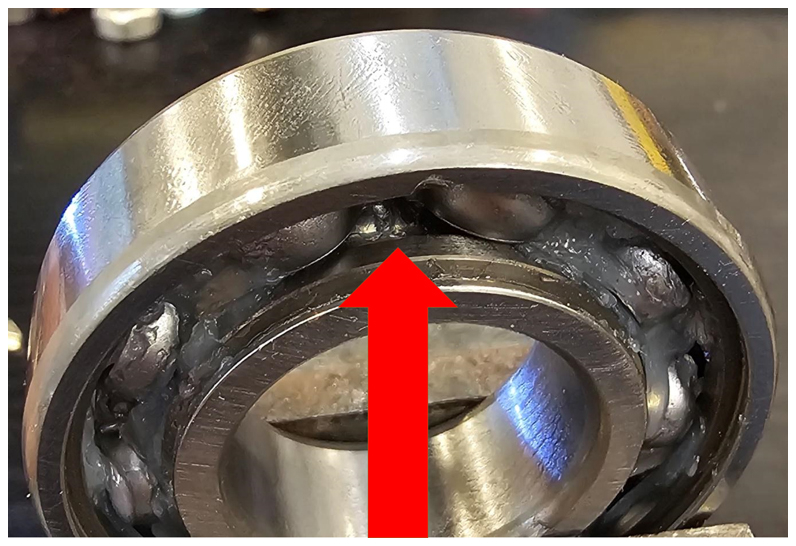
Figure 4 Outer race faults. Bearings with a damaged outer race: large fault – case 1 (left panel) and small fault – case 2 (right panel).

Table 1 Celma INDUKTA Sh90L-4 motor rated parameters.

Figure 5 Bearing with damaged inner race.

1.3 Problem definition: bi-frequency map understanding

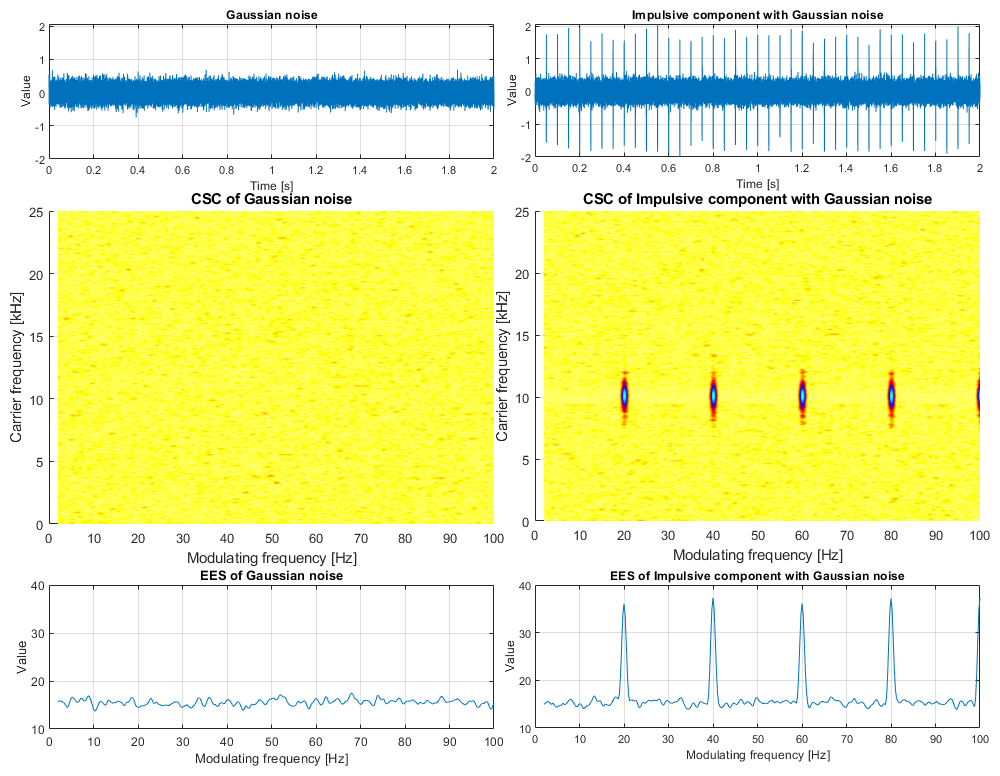
The main idea discussed here is related to the application of cyclostationary analysis to the vibration of bearings used in electric motors. We will consider both healthy and faulty bearings (encompassing various types and sizes of faults) as well as two methods of powering the motor: directly from the network and through an inverter. According to classical cases in condition monitoring, a cyclic and impulsive signal (with some background noise) subjected to cyclostationary analysis should result in a bi-frequency map with a clear signature of its periodicity (see Fig. 1, right). In the case of a lack of damage (and other cyclic sources in the measured signal), the map should not contain anything (see Fig. 1 left). In the ideal case of no-fault conditions, all values on the map should be equal to zero. In practice, there is always background noise. It may be important for detection in the early stages of damage. In the case of small modulation and resulting components with small amplitude, it might be difficult to detect the signature of damage.

Table 2 Characteristic frequencies of rolling element bearings. N₀ – shaft speed (rpm), f₀ – shaft frequency (Hz), N_b – number of rolling elements balls or rollers), d_b – ball/roller diameter, D_b – pitch diameter (center-to-center distance of rolling elements), α – contact angle.

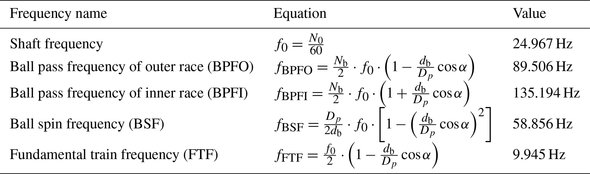
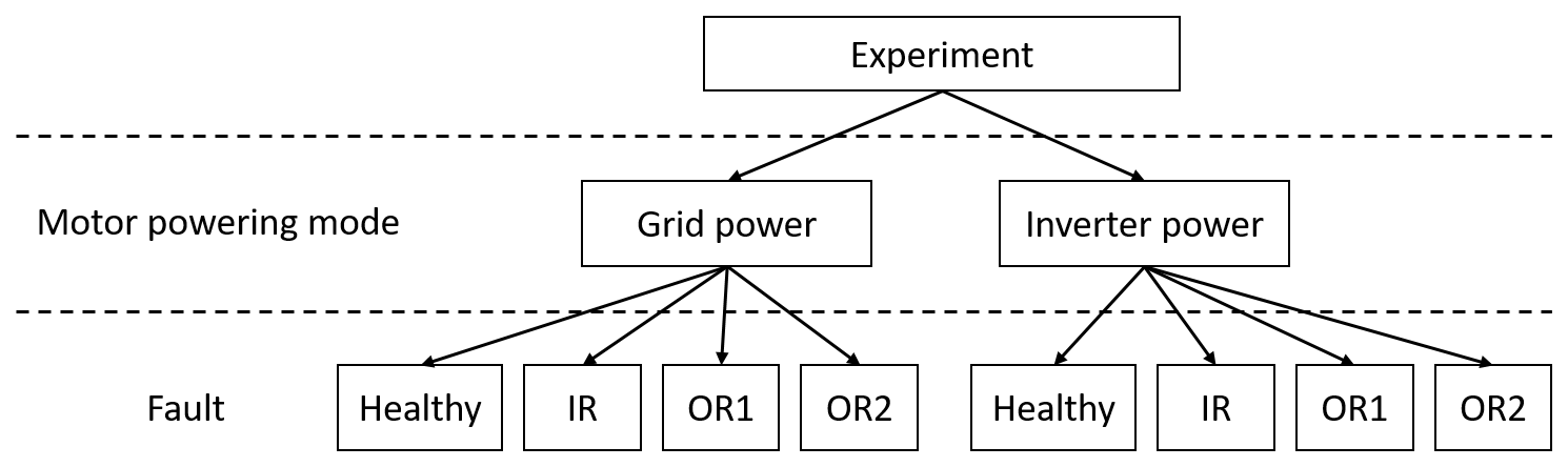
Figure 6 Plan of experimental work. IR – inner race fault, OR1 – large outer race fault, OR2 – small outer race fault.

Figure 7 Signal and its spectrogram – healthy bearing.

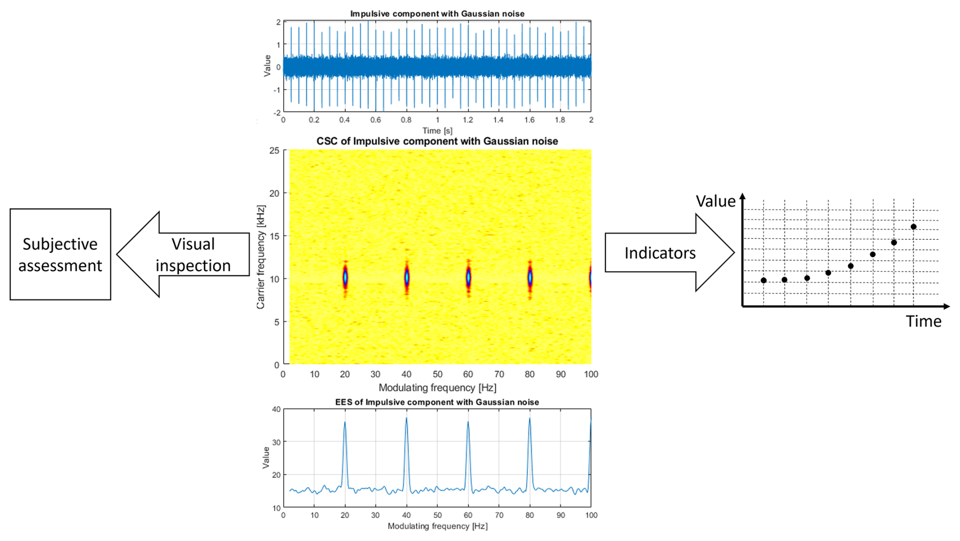
The bi-frequency map enables us to obtain two types of information: the modulating frequency (related to the cycle between impulses) and the carrier frequency associated with the natural frequency excited and modulated by periodic impulses. In the case shown in Fig. 1, modulating frequency is 20 Hz and the carrier frequency is 10 kHz. The bi-frequency map can be visually inspected, integrated into the envelope spectrum (Randall and Antoni, 2011; Mauricio et al., 2020), or serve as a basis for a novel scalar indicator that can be further monitored and used for prognosis, as shown in Fig. 2. In practical situations, visual inspection is rather difficult, subjective, time-consuming, and cannot be performed automatically. The most popular approach involves integrating the map into a one-dimensional vector, interpreted as an envelope spectrum. Unfortunately, such integration may lead to the accumulation of noise or other cyclic components in the case of a complex multicyclic signal. In the condition-monitoring system, the envelope should be further integrated to forecast the remaining useful life. Such a scalar indicator could be extracted directly from the map; however, it requires a precise understanding of all the components that exist in the map.

As mentioned, cyclostationary methods are not as widely used in the literature in the field of electric motor diagnosis. Moreover, the presented examples are rather easy to interpret. On the other hand, in this article, the authors present cyclostationary maps contaminated with additional components, allowing the reader to see that the identification and extraction of the informative component may not be straightforward. The purpose of the paper is to present, describe, and understand the structure of the spectral content of signals measured in the described scenarios. While in theory all frequency components should be known and easily interpretable, we present that it is not as obvious in practice, and even a well-suited analytical approach (cyclostationary analysis) does not paint a clear picture. It will be shown that a map can contain various components, and its interpretation and then automatic processing may be complicated. It will be highlighted that understanding all components on the map is critically important and omitting this step may lead to wrong decisions.

Figure 8 Signal and its spectrogram from bearings with an inner race fault.

Figure 9 Signal and its spectrogram from bearings with an outer race fault – much damage.

Figure 10 Signal and its spectrogram from bearings with an outer race fault – little damage.

2 Experiments and data description

2.1 Test rig description

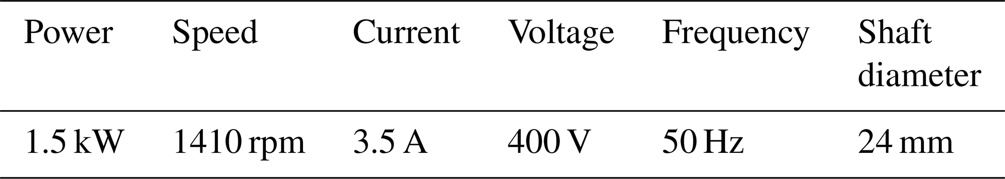
The experiment was conducted in the laboratory of the Department of Electrical Machines, Drives, and Measurements at Wroclaw University of Science and Technology. The test rig scheme is presented on the left panel of Fig. 3 and its picture on the right panel. The purpose of the experiment was to collect vibration signals from healthy and faulty bearings (SKF 6205-Z) installed in the EM. The main part of the unit is an electric motor (Celma INDUKTA Sh90L-4) coupled to another motor acting as a programmable load (PZB b44b DC). The vibration of the two bearings of the drive motor is measured using two uniaxial accelerometers (DeltaTron 4514-001) connected to a National Instruments NI-DAQmx data acquisition card: one on the counterdrive side, and the other on the drive side. Measurements were sampled at 51.2 kHz and lasted 10 s for a single signal. Parameters of this particular model of EM are presented in Table 1.

The test rig enables control of operational parameters of the EM (speed, load) as well as various faults that could be introduced by bearing replacement.

2.2 Faulty bearing description

Three cases have been considered: healthy bearing, faulty bearing with an artificially introduced outer ring fault, and faulty bearing with an artificially introduced inner ring fault. Figures 4 and 5 present pictures of damaged bearings. Bearing faults have been artificially introduced using a special micro-drill device with the appropriate drill hardness. In Table 2, basic parameters required for diagnostic procedures are presented, where BPFO is the ball pass frequency of the outer race, BPFI is the ball pass frequency of the inner race, FTF is the fundamental train frequency, and BSF is the ball spin frequency.

Several experiments have been carried out. They can be divided according to the presence of the fault (healthy, faulty), the type of fault (inner, outer), the size of the fault (no fault, small fault, large fault), and the power supply (direct grid, inverter). These variants are summarized in Fig. 6.

2.3 Results of measurements

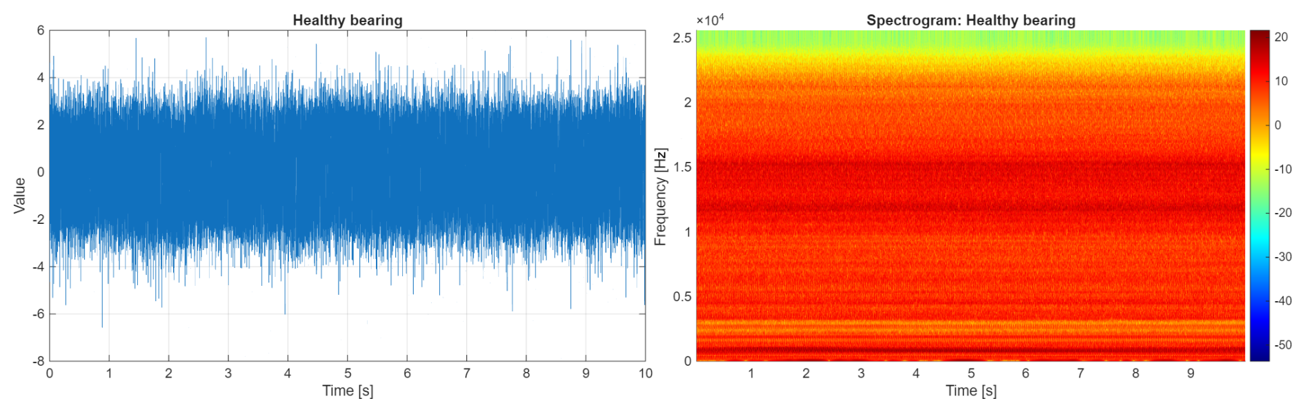
The results of each experiment are presented in the same way. First, we present the time series of each measurement (10 s in length). Second, the spectrogram of that signal is presented. The purpose of that visualization is to understand the shape of the signal in the time domain and its frequency structure, including the possible excitation of natural frequencies (an informative frequency band). All data presented in this section have been collected from the electric motor powered directly by the electric grid and from the voltage inverter. All spectrograms are presented on a logarithmic scale.

2.3.1 Grid-powered motor

In Fig. 7, the vibration signal and its spectrogram of bearings in healthy conditions are presented. It is worth noting the amplitude of the time series (which will increase for faulty cases because of the presence of impulses) and the rich and rather uniform structure of the spectral content (no dominant resonance).

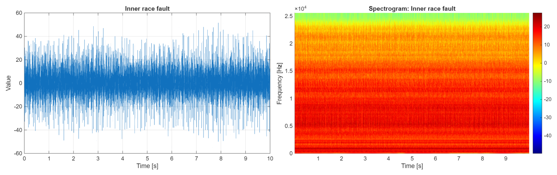
In Fig. 8, the vibration signal and its spectrogram related to a faulty bearing with an inner ring fault are presented. It is evident that the introduced fault caused a significant increase in the signal amplitudes (left panel) and a change in the spectral structure. The resonance area is visible around 5 kHz.

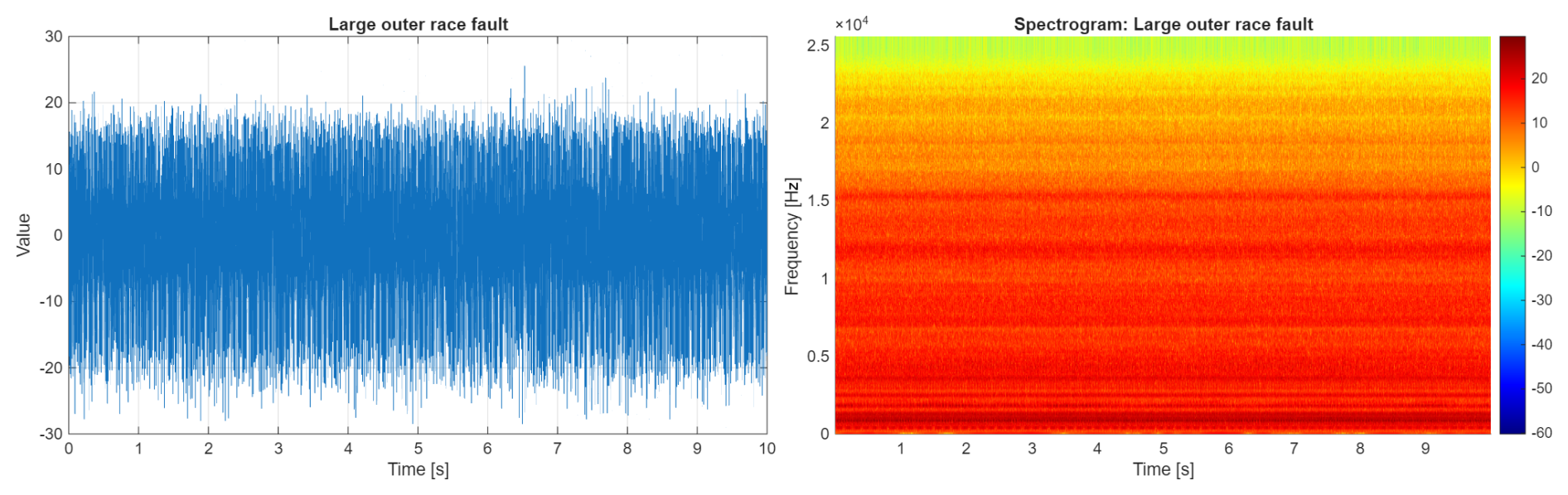
In Fig. 9, the vibration signal and its spectrogram related to a faulty bearing with a large outer ring fault are presented. Again, one may note that the introduced fault caused an increase in amplitudes of the signal (left panel), though smaller than for the inner ring. A change in spectral structure is also visible. Unfortunately, no significant pattern can be detected.

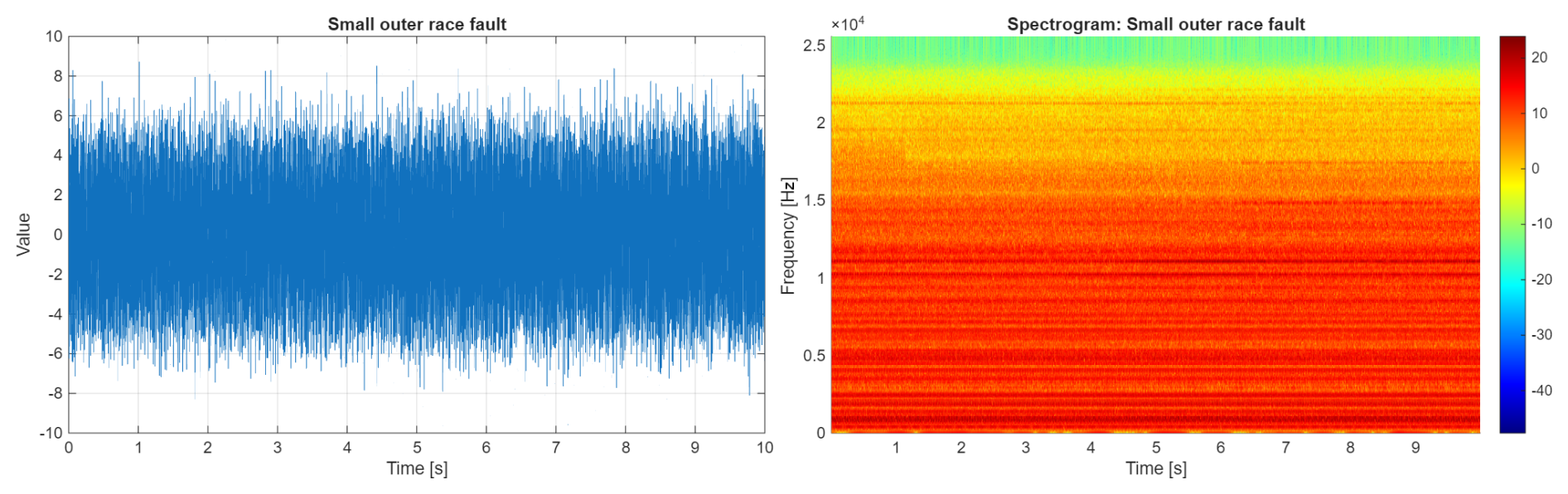
In Fig. 10, the vibration signal and its spectrogram related to a faulty bearing with a small outer ring fault are presented. An introduced fault caused a minor increase in the amplitudes of the signal (left panel), which makes the detection problem challenging (the amplitudes of informative and non-informative components are similar). No significant pattern on the time–frequency map can be detected.

2.3.2 Inverter-powered motor

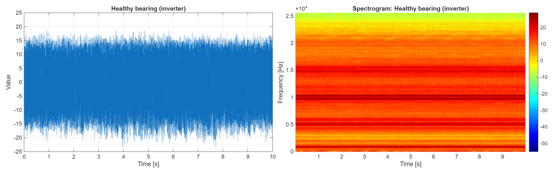
The next set of examples presents cases where the electric motor was not powered directly from the electrical grid but using a voltage inverter. In Fig. 11, the vibration signal and its spectrogram measured on healthy bearings are presented. Please note that this is the same test rig with the same motor and healthy bearings as in the previous section. The difference is just related to the change of power source. The use of the inverter significantly increased the amplitudes of the raw time series and changed the spectral structure of the signal. Two components with significantly higher amplitudes are visible on the spectrogram (5 and 10 kHz), and they are related to the set frequency modulation of the inverter.

Figure 11 Signal and its spectrogram from healthy bearings (machine driven by inverter).

In Fig. 12, the vibration signal and its spectrogram are presented. These are related to a bearing that is faulty with a fault of the inner ring. It is worth noting that the introduced fault caused a significant increase in amplitudes of the signal (left panel) and a change in the spectral structure (in comparison to a healthy motor driven by an inverter, as well as a healthy motor powered by an electric grid). The resonance area is barely visible around 5 kHz.

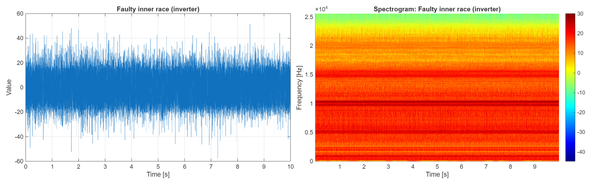
Figure 12 Signal and its spectrogram from bearings with a faulty inner ring (machine driven by inverter).

In Fig. 13, the vibration signal and its spectrogram related to a faulty bearing with a large outer ring fault are presented. As in previous cases, an introduced fault caused an increase in signal amplitudes (left panel), however, smaller than for the inner ring. Any significant changes in the spectral structure or pattern can be detected.

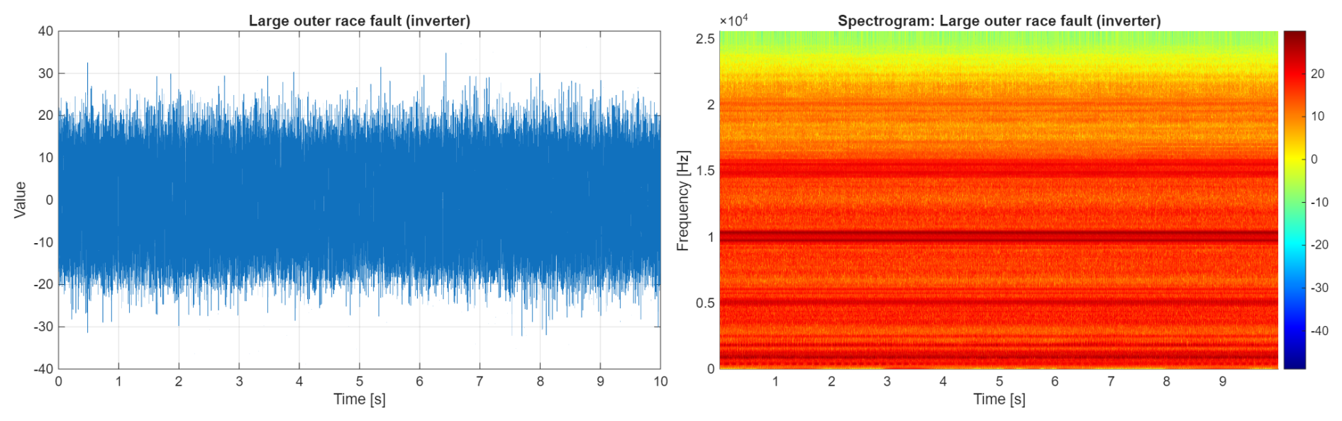
Figure 13 Signal and its spectrogram from bearings with an outer race fault – much damage (machine driven by inverter).

In Fig. 14, the vibration signal and its spectrogram related to a faulty bearing with a small outer ring fault are presented. An introduced fault caused a minor increase in amplitudes of the signal (left panel), which makes the detection problem challenging (the amplitudes of informative and non-informative components are similar). Any significant pattern on the time–frequency map can be detected.

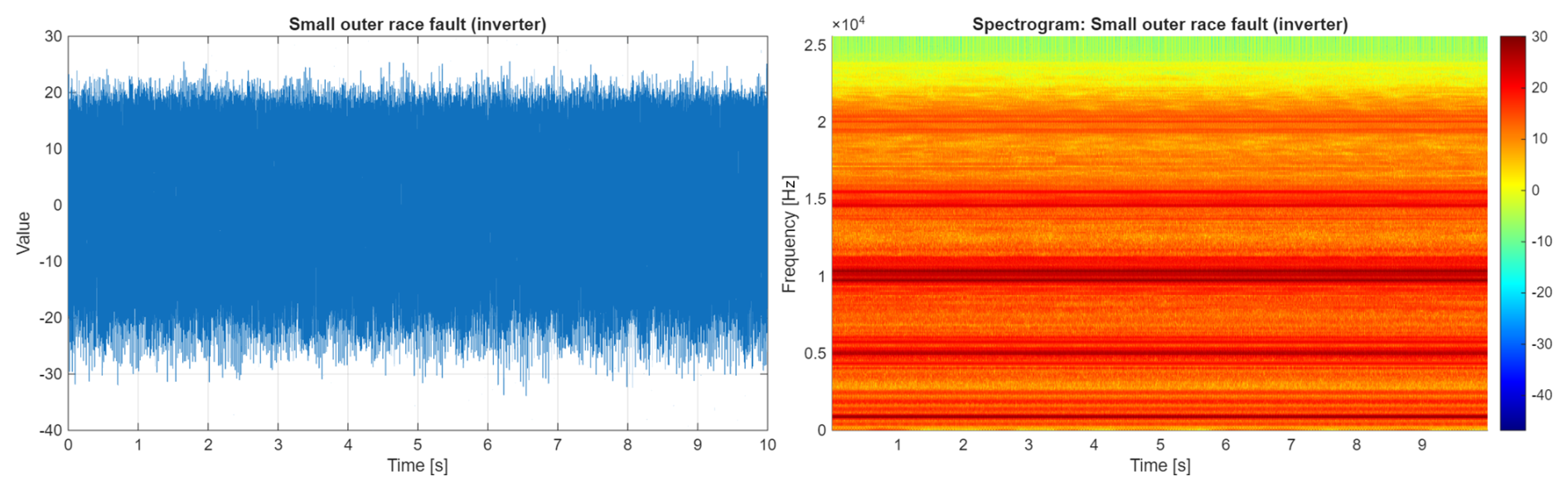
Figure 14 Signal and its spectrogram from bearings with a faulty outer ring – small fault (machine driven by inverter).

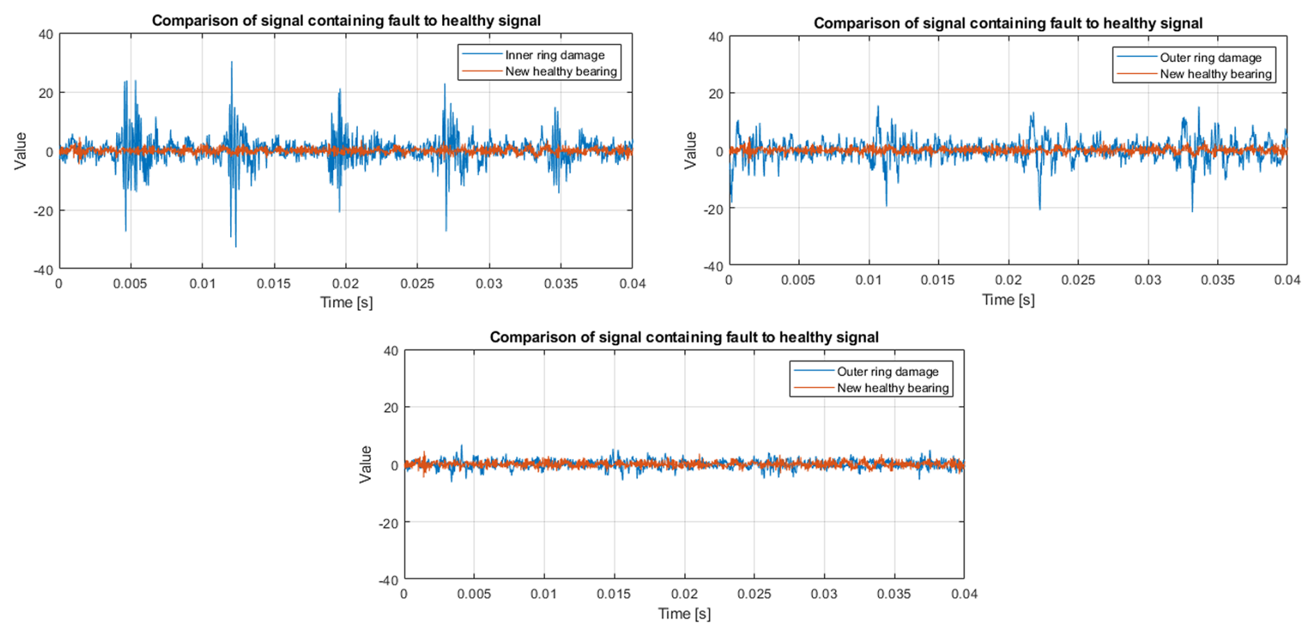
2.3.3 Healthy vs. faulty bearings: comparison of signals

Introducing artificial damage to the bearings is not a natural degradation process. Created damages cause a significant increase in amplitudes, especially related to cyclic impulses. In Fig. 15, a signal comparison is presented: each graph shows a signal from the good-condition bearing used as a reference and a signal from the defective bearing. It is clear now that the increase in amplitudes mentioned earlier is related to high-amplitude impulses. The inner race fault brings about a large impulsive component. The smaller outer ring fault provides smaller impulses in comparison to the large outer race fault.

Figure 15 Comparison of healthy and faulty signals for grid-powered setup.

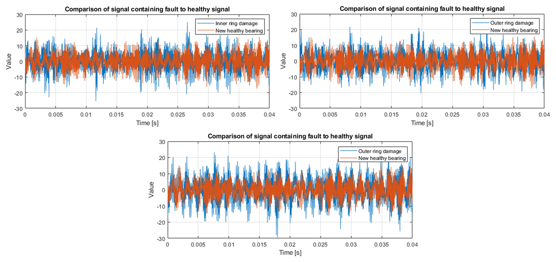
In Fig. 16, a similar comparison of signals is presented; however, this time we consider experiments carried out with the motor driven by the inverter. Each plot displays a signal from a bearing in good condition, used as a reference, and a signal from a faulty bearing. As in this case, signals contain much more background noise, and the increase mentioned above is not critical. An impulsive component is masked by background noise, and the presence of impulses is not so clear as in a grid-powered case. One may conclude that even if the fault size is large and is clearly visible in the time domain for EM powered by the grid, in the case of the inverter, detection may not be as straightforward. For an early-stage fault, it could be a real challenge.

Figure 16 Comparison of healthy and faulty signals for the inverter-powered setup.

3 Cyclostationarity modeling for vibration analysis

In this section, basic definitions of cyclic spectral coherence is presented, while some indicators used for comparing approaches will be recalled in the Appendix B.

Cyclic spectral coherence (CSC) is a well-known bi-frequency representation often used to investigate the cyclostationary aspects of time series {X_t}. It is defined as a double Fourier transform calculated on the instantaneous autocovariance function, such as Antoni (2007):

$$\begin{array}{}\text{(1)}& C_X(f,\mathit{ϵ})={\displaystyle \frac{S_X(f,\mathit{ϵ})}{\sqrt{S_X(f+\mathit{ϵ}/\mathrm{2},\mathrm{0})S_X(f-\mathit{ϵ}/\mathrm{2},\mathrm{0})}}},\end{array}$$

where

$$\begin{array}{}\text{(2)}& S_X(f,\mathit{ϵ})=\underset{N\to \mathrm{\infty }}{lim}{\displaystyle \frac{\mathrm{1}}{N}}\sum _{t=-N}^N\sum _{\mathit{\tau }=-\mathrm{\infty }}^{\mathrm{\infty }}{R}_X(t,\mathit{\tau })e^{-i\mathrm{2}\mathit{\pi }f\mathit{\tau }}{e}^{-i\mathrm{2}\mathit{\pi }\mathit{ϵ}t},\end{array}$$

where ϵ is the cycle frequency and $R_X(t,\mathit{\tau })=\mathbb{E}{X}_t{X}_{t-\mathit{\tau }}$ is the autocovariance function of time series {X_t}. In this application, f can be understood as the carrier frequency and ϵ as the modulating frequency, both expressed in Hz. S_X(f,ϵ) is estimated using averaged cyclic periodogram (ACP) (Antoni, 2007).

It is important to remember that in practical implementation, the estimator of the CSC is calculated for time series $\mathit{x}=\mathit{\{}{x}_{\mathrm{1}},x_{\mathrm{2}},\mathrm{\dots },x_N\mathit{\}}$ of length N. There are many approaches for estimating CSC, but the most popular method (also used in this article) is based on the averaged cyclic periodogram. It results in the calculation of the bi-frequency map ${\widehat{C}}_X(f,\mathit{ϵ})$, where f∈ℱ and ϵ∈ℰ.

If one can assume that the model of the investigated signal x displays cyclostationary properties, then one could observe the modulation fringes (individual vertical lines visible on the CSC map) located at specific modulating frequencies ${\mathit{ϵ}}_{\mathit{l}}=\mathit{\{}{\mathit{ϵ}}_{l_{\mathrm{1}}},{\mathit{ϵ}}_{l_{\mathrm{2}}},\mathrm{\dots },{\mathit{ϵ}}_{l_P}\mathit{\}}$ representing the fundamental frequency of modulation (called fault frequency) and its harmonic multiples. Those fringes typically occupy a limited carrier frequency band f_f∈ℱ called the informative frequency band (IFB).

4 Results of cyclostationary analysis and their interpretation

In this section, the authors present the results of the cyclostationary analysis of the described signals. The bi-frequency maps enable us to visualize the data more clearly and understand their character. They also allow us to describe the differences between the signals.

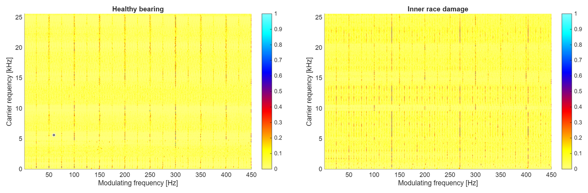
Figure 17 presents CSC maps calculated based on signals from a healthy bearing (panel a) and from a bearing with an inner race fault (panel b). The signal from the healthy bearing contains one major component visible on the map: a cycle of 24.97 Hz and its multiples. This component describes the rotational frequency of the motor shaft.

The signal from the bearing with the inner race fault presents a more complicated structure. Similarly to the healthy bearing, we can observe the component at 24.97 Hz and its multiples; however, the predominant cycle has a frequency of 135.2 Hz (and its multiples), which correctly corresponds to the inner race fault. In this signal, sidebands also appear on the CSC map. For example, the component at 110 Hz is clearly visible on the map, and this component is the first left-hand sideband of the central frequency of 135 Hz (inner race fault) with a distance of 25 Hz (shaft cycle).

Figure 17 CSC maps for signals – grid power.

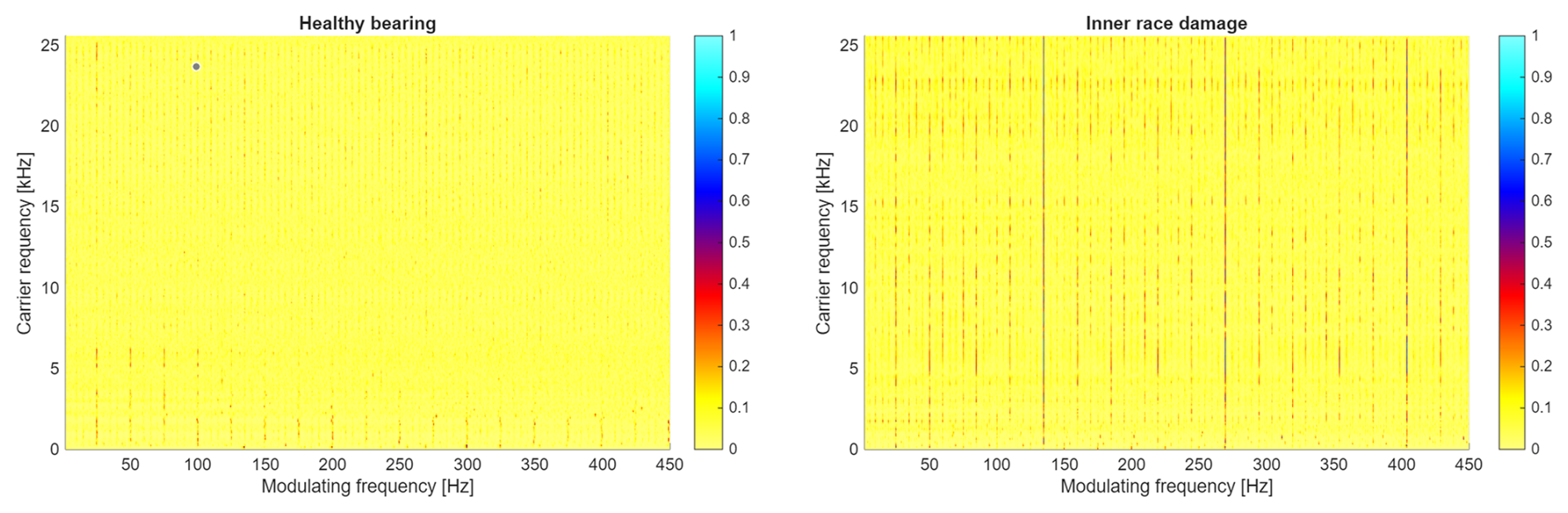
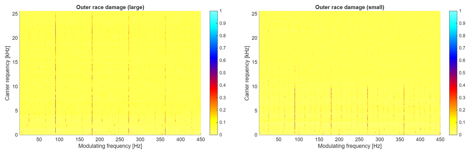
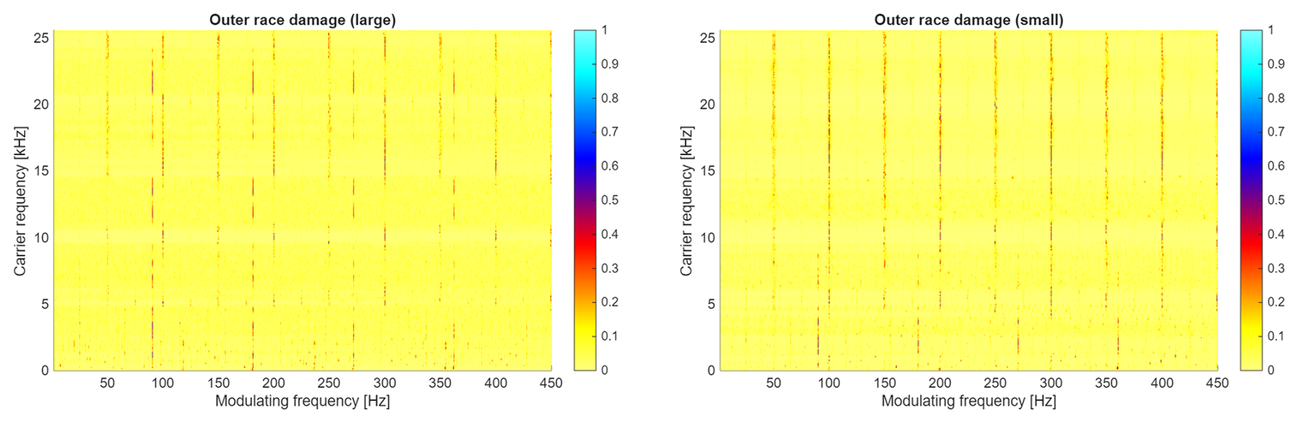
Figure 18 presents CSC maps calculated based on signals from bearings with large (panel a) and small (panel b) outer race faults. On both maps, the predominant component describes the 89.5 Hz cycle (and its multiples) that correctly describes the characteristic frequency of the outer race fault. The main difference between those two faults is clearly visible on the maps. It manifests mainly as a difference in the carrier frequency band occupied by the fringes describing the fault component. The value of the fringes also differs and is stronger for the larger fault.

Figure 18 CSC maps for signals – grid power.

Unfortunately, the structure of the bi-frequency map for all experiments with an inverter-powered motor is significantly different (see Figs. 19 and 20). A dominant component on the map is related to 50 Hz and is harmonics (100, 150, etc.). These components are critical for the small outer bearing fault case where the map is completely dominated by 50 Hz and the fault signature is barely visible (limited band, smaller amplitudes). One may conclude that the same fault is much more difficult to detect in the case of using an inverter.

Figure 19 CSC maps for signals – inverter power.

Figure 20 CSC maps for signals – inverter power.

Figures 21 and 22 present the enhanced envelope spectra (EES) calculated based on CSC maps from Figs. 17, 18, 19, and 20. This representation allows us to observe and interpret the information more simply and directly. Furthermore, those plots allow us to confirm and emphasize the information presented on the CSC maps.

Figure 21 presents the EES plots for signals measured using a grid-powered setup. Regarding the signal from a healthy bearing, only the four shaft-related components can be observed (the rest are masked by other components). The EES related to the inner race fault exhibits clear peaks that describe the fault. One can also identify peaks at the first three harmonic frequencies related to the shaft cycle, as well as sidebands around fault harmonics that are related to the shaft cycle (i.e., 135 Hz ± 25 Hz). A similar situation can be observed at EES plots regarding both outer race faults. Peaks describing fault harmonics are clearly visible above all other components. One can identify two or three shaft-related harmonics, and shaft-related sidebands can also be observed.

Figure 21 Enhanced envelope spectrum of signals measured on a grid-powered motor.

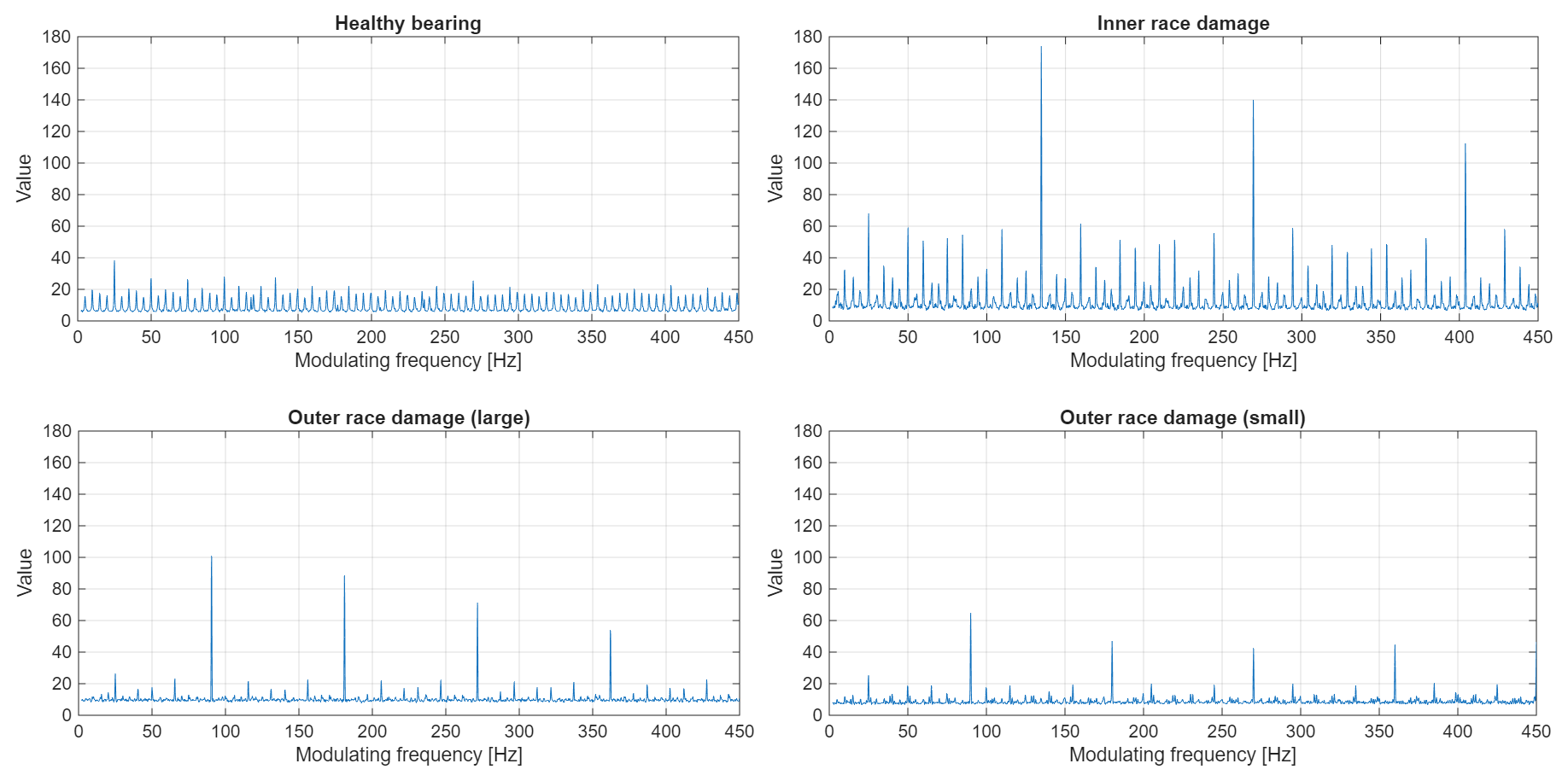
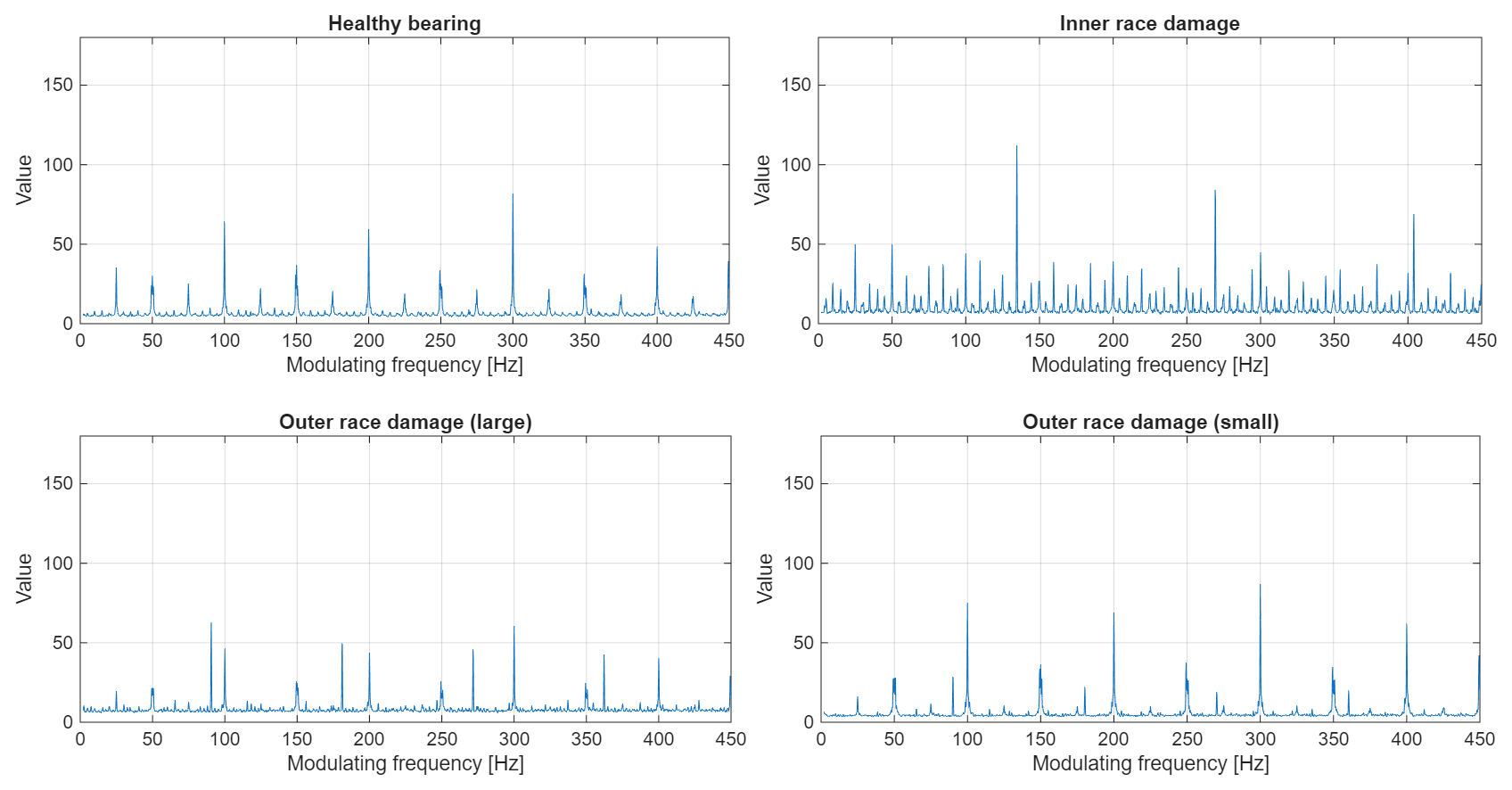
Figure 22 presents the EES plots for signals measured using an inverter-powered setup. Regarding signal from a healthy bearing, the situation is similar to the grid-powered setup (shaft-related frequencies are visible), but in this case, components at multiples of 50 and 100 Hz are significantly stronger than all other multiples of 25 Hz. For the inner race fault, the structure of EES for grid power and inverter power is very similar; however, for inverter power, the overall scale of EES is visibly smaller. On the other hand, the EES plots for both outer race faults are significantly different from those for grid-powered scenarios. Besides the same fault-related components that are visible in grid-powered case, now one can observe a significant presence of frequencies that are multiples of 100 and 50 Hz, with a structure similar to the one observed at the EES of a healthy bearing (multiples of 100 Hz are significantly stronger than multiples of 50 Hz). However, fault-related components are still clearly visible.

Figure 22 Enhanced envelope spectrum of signals measured on inverter-powered motor.

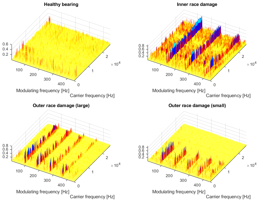
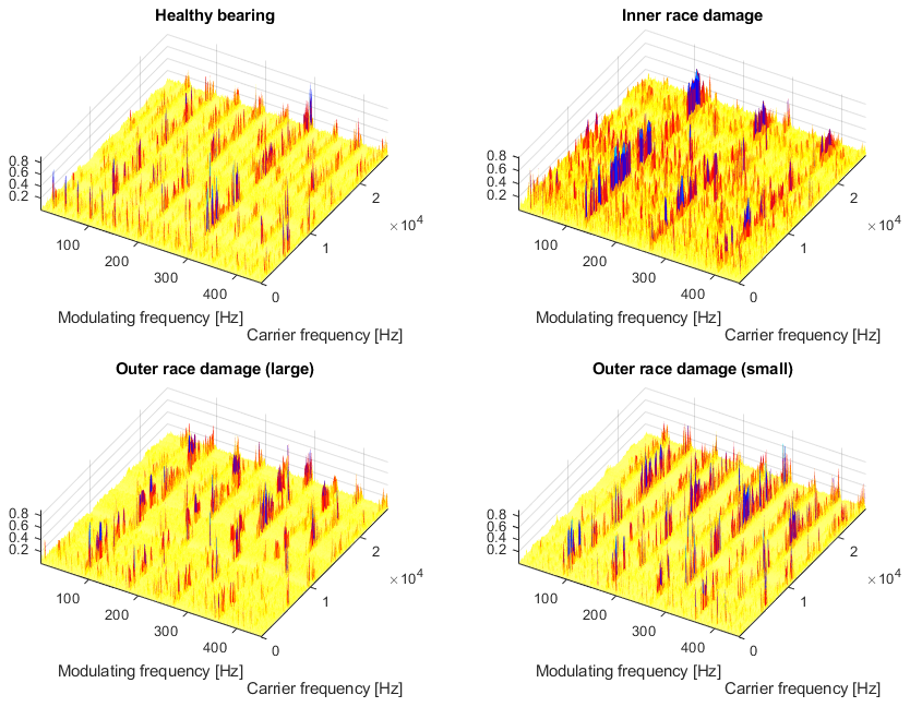
Figures 23 and 24 present the same CSC maps as shown before but with a three-dimensional viewing perspective. Such a viewing mode allows us to visualize better the relation between the values of noise floor fluctuations (non-informative areas) and the values of the actual modulation-related fringes at the expected modulation frequencies (informative areas). Especially for cases of inner ring fault (for both grid and inverter power) one can see that there are values of significant amplitudes scattered all over these maps. It is an important observation since, for further investigation of such cases, one might need to incorporate additional steps in the processing procedure, such as denoising or filtration. However, the remaining cases (healthy bearings or outer race faults) seem to produce much cleaner CSC maps with significantly less contaminated, non-informative areas.

Figure 23 CSC maps for signals – 3D view (grid power).

Figure 24 CSC maps for signals – 3D view (inverter).

In Fig. 25, a basic feature is presented that accumulates all the information into one value. One can see that introducing a fault in the bearing causes an increase in amplitudes on the map, indicating that the value of the feature is higher than in a healthy state. A small outer race fault provides a relatively small increase in the value of the feature. It is worth noting that even under good conditions, there are many components with relatively small amplitudes (related to the shaft and others), so their accumulation results in relatively high background noise.

Another interesting observation can be made: although inverter-powered scenarios seem to produce CSC maps and EES spectra that contain significantly more components in relation to the grid-powered scenarios, a comparison of the four inverter-powered cases with respective grid-powered cases shows that the overall sums of value aggregation are lower.

Finally, one can make a third observation: for the grid-powered case, a small fault of the outer race produces a sum value that is minimally larger than for the healthy bearing. However, in the case of the inverter-powered scenario, the same low-level fault of the outer race produces a sum value that is significantly lower than for the healthy bearing. In particular, for a grid-powered scenario, the difference in values is equal to 3.58×10², which constitutes a positive difference of 1.85 %. However, for an inverter-powered scenario, the difference in values is equal to 2.34×10³, which represents a negative difference of 15.49 %.

Figure 25 Sums of values within the eight CSC maps.

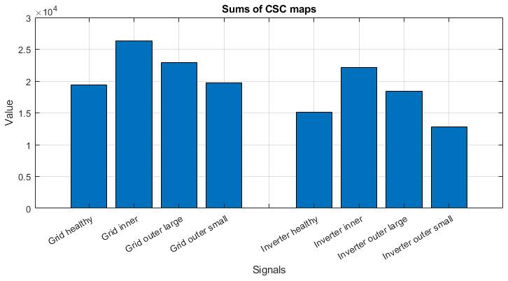
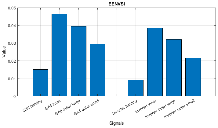
Figure 26 presents the values of the EENVSI indicator for the eight cases presented. One can make two clear observations, as follows.

1. For both grid-powered and inverter-powered cases, signals measured on faulty bearings produce higher values of EENVSI than signals measured on healthy bearings.

2. Signals describing inverter-powered cases produce lower values of EENVSI than for grid-powered cases. Since EENVSI (as well as ENVSI) is conceptually equivalent to SNR but for envelope spectra instead of signals, one can conclude that this is further evidence that an inverter-powered scenario produces signals more contaminated with spectral components not related to the faults.

Figure 26 EENVSI values for the eight presented cases.

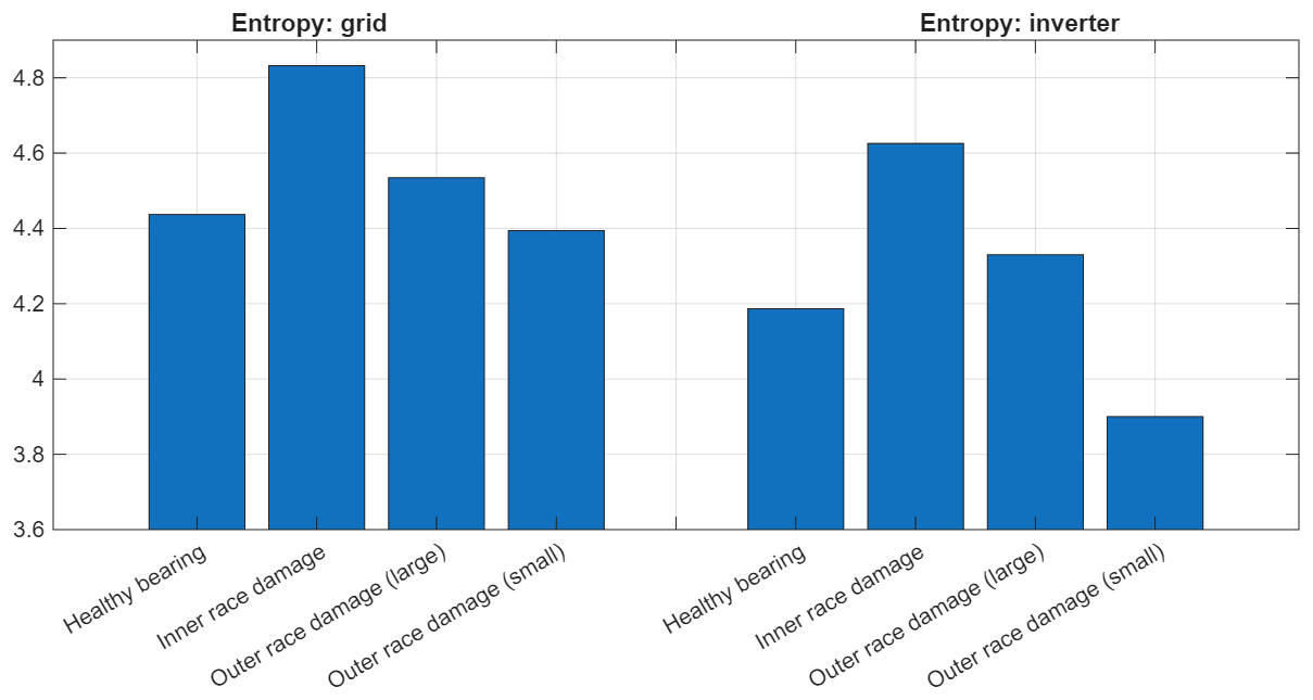
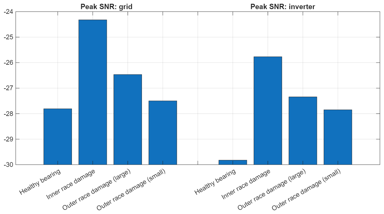
Similarly to the EENVSI, Fig. 27 shows that the entropy of the CSC maps also takes lower values for configurations with the inverter compared to the grid-power setup for all four scenarios (Gonzalez et al., 2020). The same effect can be observed for peak SNR in Fig. 28.

Figure 27 Entropy values for the eight presented cases.

Figure 28 Peak SNR values for the eight presented cases.

5 Discussion

Even an electric motor with good-condition bearings produces a cyclostationary signal with a complicated harmonic structure. Introducing a fault to the bearing delivers cyclic components related to the frequency of the fault (inner, outer). The amount of damage influences the structure of the map. One may summarize that for electric motors powered by the electric grid, bearing fault detection is not so complicated; however, it requires the smart integration of the kind of envelope spectrum or even the extraction of scalar features. Unfortunately, an electric motor driven by an inverter seems to be much more challenging. The inverter produces a significantly higher level of raw signal, which masks the informative component related to the damaged bearing. Moreover, a bi-frequency map contains a family of components with much higher amplitudes than the fault signature. The relation between informative and noninformative components is much worse in the case of a motor driven by an inverter. One may observe that an inverter introduces numerous non-informative components, which decrease the signal-to-noise ratio. What is important is that the estimated amplitudes of fault components are smaller in the case of a motor driven by an inverter. This means that disturbances introduced by the inverter increase background noise (noninformative components) but also influence values of informative components that may have critical importance for decision-making.

Our observations open up new research directions related to the development of smart integration into the envelope spectrum and the statistical analysis of the map to detect informative components.

6 Conclusions

Cyclostationary analysis is well-known in the condition-monitoring community; however, its application in bearing diagnostics for electric drives has not been as frequent until now. Several journal papers proposed methods based on the cyclostationary approach; however, none of them deeply studied the structure of the CSC map before the stage of feature extraction and decision-making.

In this paper, the authors conducted a simple experiment in the lab using a test rig driven by a grid and an inverter. Four different bearing conditions have been investigated (healthy, inner race fault, small outer race fault, and large outer race fault). The purpose of this work was to study the structure of the map and to investigate the feasibility of utilizing basic features that can be extracted from it.

It was observed that the source of energy for the electric drive is critically important for cyclostationary analysis. The inverter introduces non-informative components (from a fault detection perspective) that make the map less readable. Furthermore, the amplitudes of the components related to the fault frequency are smaller than in the case powered by the grid. Additionally, some additional components related to the shaft imbalance have been identified. These facts require a redefinition of the feature-extraction procedure and a robust fault detection method.

It has been confirmed that introducing damage to the tested bearings generates components on a bi-frequency map at the fault frequency and its harmonics. The structure of the spectral signature of the fault follows the theoretical expectation. An increase in the size of the fault leads to an increase in the signature. In this paper, it has been shown that this is not exactly the case for an electric motor powered by an inverter. In general, the rule remains valid but cannot be applied directly to the grid and inverter cases. Moreover, a signature integrated to the 1D scalar value showed that a small outer fault provides a signature smaller than that of healthy conditions. Even though the global cyclostationary indicator is slightly smaller for the inverter case, the normalized feature (EENVSI) showed significantly worse performance for the inverter-driven motor. The normalized cyclostationary indicator enables tracking fault development; however, its values for the inverter are smaller than those for the grid case. This means a smaller effectiveness of fault detection in this case.

It was believed that cyclostationary analysis is suitable for detecting mechanical faults in rolling bearings, as it can easily identify a nonlinear interaction between the modulating frequency (related to the fault) and the carrier frequency (related to the natural frequency). The amplitude of the component on the bi-frequency map should be proportional to the size of the fault. It should not depend on the type of power supplier.

Cyclostationary analysis for vibration signals from rolling element bearings in electric drives with inverters requires deep investigation into the interpretation of the structure of the map and feature-extraction procedures. It is noteworthy that it cannot be a simple aggregation that globally assesses the map (such an approach could be interesting from the perspective of online condition-monitoring systems). Even classical integration procedures that transform a 3D map to a 2D envelope spectrum may provide an accumulation of disturbances and decision-making with high uncertainty. In the considered cases, it has been observed that the additional components are wideband and significantly visible in the maps, which makes a lot of standard approaches unsuitable (i.e., IFB selection, considering the strongest cyclic components, etc.). Additionally, it has been observed that even the same configuration powered by the grid or by the inverter presents very different characteristics, and even parameterization with appropriate metrics shows that they cannot be analyzed in the same way (i.e. different decision thresholds are required, different class separation intervals can cause a different classifier to be required, etc.). The contribution of this paper lies in explaining the structure of CSC map in a scenario of the diagnostics of bearings in the induction motors (operating with and without an inverter), and it can be considered a very preliminary step for proposing automatic diagnostic techniques.

Appendix A: List of abbreviations

Abbreviation	Full name
AIS	amplitude of informative signal
BPFI	ball pass frequency over inner race
BPFO	ball pass frequency over outer race
BSF	ball spin frequency
CSC	cyclic spectral coherence
EENVSI	enhanced envelope spectrum-based indicator
EES	enhanced envelope spectrum
EM	electric motor
EMI	electromagnetic interference
ENVSI	envelope spectrum-based indicator
ES	envelope spectrum
FTF	fundamental train frequency
IES	improved envelope spectrum
IFB	informative frequency band
IR	inner ring
OR	outer ring
REB	rolling element bearing
SES	squared envelope spectrum
SNR	signal-to-noise ratio

Appendix B: Definition of indicators

B1 Sum of CSC – a global indicator of cyclostationarity

Since the CSC map is a correlational representation, one can assume that non-informative areas will be occupied by low correlation values (theoretically, they should tend to zero; practically, there are some “noise” components below 0.2). On the other hand, informative fringes that describe modulation effects will be represented by higher correlation values (typically above 0.6). From this assumption, it can be argued that the total sum of all of the values on the map can be a simple indicator of the number of modulation effects present on the map, without requiring any prior knowledge about the particular frequencies of interest.

The indicator M can be defined as

$$\begin{array}{}\text{(B1)}& M=\sum _{f\in \mathcal{F}}\sum _{\mathit{ϵ}\in \mathcal{E}}\left|C_X(f,\mathit{ϵ})\right|.\end{array}$$

B2 An integrated EES

The enhanced envelope spectrum (EES) is a representation equivalent to the envelope spectrum in terms of the information provided (Randall et al., 2001) but calculated based on the CSC map. It is obtained by aggregating the map along the dimension of the carrier frequency domain, such as

$$\begin{array}{}\text{(B2)}& \mathrm{EES}\left(\mathit{ϵ}\right)=\sum _{f\in \mathcal{F}}\left|C_X(f,\mathit{ϵ})\right|,\end{array}$$

where ϵ∈ℰ.

B3 ENVSI and its adaptation to 3D map

Envelope spectrum-based indicator (ENVSI) is a scalar indicator calculated based on the envelope spectrum to describe the energy content of harmonic fringes related to a particular modulating component in relation to the energy of the envelope spectrum in a given frequency range (Hebda-Sobkowicz et al., 2020b). However, while in the original article, the base representation for ENVSI is squared envelope spectrum (SES), in this implementation (that we could call EENVSI – enhanced envelope spectrum-based indicator), the base is EES described in Sect. B2, such as

$$\begin{array}{}\text{(B3)}& \mathrm{ENVSI}={\displaystyle \frac{{\sum }_{i=\mathrm{1}}^K{\mathrm{AIS}}_i}{{\sum }_{j=\mathrm{1}}^N{\mathrm{SES}}_{{\mathit{ϵ}}_j}}},\end{array}$$

where AIS stands for the amplitudes of the information signal described by the components of fault frequency, K is the number of informative components, and N is the length of the squared envelope spectrum (SES). Hence, for the calculation of ENVSI, the SES is trimmed such as ${\mathrm{AIS}}_K={\mathrm{SES}}_{{\mathit{ϵ}}_N}$. Consequently,

$$\begin{array}{}\text{(B4)}& \mathrm{EENVSI}={\displaystyle \frac{{\sum }_{i=\mathrm{1}}^K{\mathrm{AISE}}_i}{{\sum }_{j=\mathrm{1}}^N{\mathrm{EES}}_{{\mathit{ϵ}}_j}}}.\end{array}$$

It is important to note that in the numerators, AIS for ENVSI is selected from the squared envelope spectrum, and AISE (AIS for EENVSI) is selected from EES.