Study on the stability of analytical periodic solutions of nonlinear gear systems

The gear system with backlash is a strong nonlinear system. The generalized harmonic balance method is capable of dealing with most strong nonlinear problems. The analytical solutions of unstable periodic motion and quasi-periodic motion can also be obtained, and the principle of chaos generation can be further explained. The present study employs the generalized harmonic balance method to obtain an approximate analytical solution for a nonlinear gear dynamic system, which can be used to analyze the dynamics models of gear system with backlash. The accuracy of the analytical solution can be controlled by changing the number of harmonic terms. A characteristic diagram of harmonic amplitude versus the amplitude of the dynamic transmission error (DTE) is obtained using the generalized harmonic balance method, and the influence of DTE on the stability and bifurcation of the system is discussed. The stable intervals and bifurcation of periodic motion of the system are discussed in detail through the analysis of eigenvalue structures. It is found that the existence of Hopf bifurcation at the intersection of stable and unstable branches of periodic solutions leads to changes in the topology of periodic motion of the system.

1 Introduction

Gear transmission is widely used in various industries in human society, and its smooth operation is crucial for the entire system. Backlash is the inherent characteristic of the gear transmission system. In the split torque transmission system of helicopter main reducers in particular, the meshing periodic motion of branch spur gears directly affects the vibration characteristics of the system. The existence of this backlash can cause gear impact phenomena and lead to a series of nonlinear behaviors in the system (Liu et al., 2022; Qi et al., 2023). The stability of periodic motion is an important part of the study of nonlinear system dynamics behavior, which includes both the stability of parameters and the stability of initial perturbations (Natsiavas, 2019; Huang and Fu, 2019). The traditional harmonic balance methods can only study nonlinear systems with small parameters; that is, weak nonlinear systems and the time multi-scale method and perturbation method cannot directly discuss the stability of periodic motion solutions. Luo and Huang (2011) proposed a generalized harmonic balance method in 2012. The Fourier series with time-varying coefficients is used to represent the periodic solution of the system. The original nonlinear system is replaced by a differential equation with coefficients. The stability of the solution is determined by the eigenvalues of the Jacobian matrix of the coefficient differential equation, and the precision of the solution can be controlled by changing the number of harmonic terms. Through Hopf bifurcation, the mechanism of multi-period bifurcation can be deduced theoretically, and the principle of chaos generation can be further explained.

Figure 1 The dynamical model of the gear meshing system.

The analytical solutions of gear systems have been studied by scholars in the past. In 1992, Padmanabhan and Singh (1992) studied gear systems with backlash and used the harmonic balance method, numerical methods, and computer simulations to prove the existence of harmonic, periodic, and chaotic solutions. They constructed approximate solutions for excitation frequencies using the harmonic balance method, which were then used to classify weak, moderate, and strong nonlinear spectral interactions. In 1995, Blankenship and Kahraman (1995) attempted to explain the complex behavior of steady-state forcing responses commonly observed in rotating machinery using harmonic balance methods and experimental verification. In 2005, Al-shyyab and Kahraman (2005) obtained analytical solutions for period-1 and sub-harmonic motions in multi-pair gear trains using the harmonic balance method and applied the Floquet theory to determine the stability of the periodic solutions. However, these studies generally ignore the strong nonlinear characteristics of the system and often only apply to some specific low-speed and low-dimensional gear systems.

Since its birth, the application of the generalized harmonic balance method in the field of nonlinear dynamics has attracted the attention of many scholars. Luo and Huang (2013) and Huang and Luo (2014, 2015) analyzed period-m motion in the Jeffcott rotor system using the generalized harmonic balance method, provided analytical expressions for the system's periodic solutions, and analyzed the stability and bifurcation of period-m motion. Huang and Fu (2019) determined the vector field of the subsystem using discontinuity theory, explained simulated periodic motion and chaotic motion using the generalized harmonic balance method, and discussed periodicity and stability of steady-state motion. Luo and Huang (2013), Xu et al. (2017), and Huang and Luo (2014, 2015) used the generalized harmonic balance method to obtain an analytical solution for periodic motion in a class of one-dimensional nonlinear dynamic systems and used eigenvalue analysis to determine the stability and bifurcation of the system's periodic motion. Then, Xu et al. (2022, 2023, 2024), studied a nonlinear rotor system and found a sequence of odd-order independent sub-harmonic vibrations being released for vibration isolation and suppression. The frequency–amplitude characteristics of independent sub-harmonic vibrations were discussed by the generalized harmonic balance method. They provided a bifurcation tree from period 1 to period 8 using the amplitude–frequency characteristics and completed numerical simulations of stable period-1 to period-8 evolution to verify the accuracy of the periodic evolution (Luo and Guo, 2018). Luo and Huang (2012) used the generalized harmonic balance method to obtain the analytical solutions for period-m flows and chaos in nonlinear dynamical systems, which they presented. The nonlinear damping, periodically forced, Duffing oscillator was investigated as an example to demonstrate the analytical solutions of periodic motions and chaos, with the mechanism for a period-m motion jumping to another period-n motion in numerical computation founded.

Figure 2 The fitting curve of the function of gear backlash.

At present, there are some studies on the period and motion stability of nonlinear gear system. Margielewicz et al. (2017) introduced the computer simulation results of the time change gear model, and in order to determine the scope of irregular gear behavior, the branch of the branch of the Lyapunov index and amplitude frequency distribution was drawn using the numerical method. Farshidianfar and Saghafi (2014) conducted an analytical and numerical study of bifurcation and path to chaos in gear systems. Applying the Melnikov analytical method, the threshold values for the occurrence of chaotic motion are obtained. The numerical simulation of the system including the bifurcation diagram, phase plane portraits, Fourier spectra, and time histories is considered to confirm the analytical predictions for the occurrence of homoclinic bifurcation and chaos in nonlinear gear systems. In recent years, research on the nonlinear behavior of gear backlash has mostly been based on numerical methods. Mo et al. (2024) utilized phase trajectory planes, phase diagrams, Poincaré maps, and bifurcation diagrams to describe the nonlinear behavior of the system. They employed the multi-scale method to analyze the system's superharmonic resonance characteristics and determined the stability conditions for superharmonic resonance through numerical analysis. Hu et al. (2023) calculated the time-varying meshing stiffness (TVMS) based on slicing theory and numerical computation methods. Using the Runge–Kutta method, they analyzed the periodic, sub-harmonic, and chaotic behaviors of the system while also validating the effectiveness of their computational approach.

In this paper, based on the classical nonlinear dynamics model of a single gear pair with backlash, the generalized harmonic balance method is used to search the periodic motion of a gear system with given parameters and determine its stability. The stability and bifurcation of periodic solutions will be analyzed using eigenvalue structure analysis. The analytical results will be compared with numerical solutions to verify the accuracy of the analytical results. In addition, the periodic motion of the gear system is studied through the harmonic amplitude and phase diagram, and the stability is determined. The stability of the strong nonlinear single-stage gear system with periodic motion is studied to provide a reference for selecting the corresponding parameters and initial conditions of the target periodic solution.

2 Nonlinear gear dynamics model with backlash

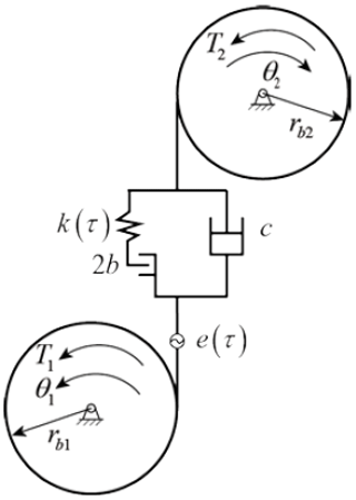
The dynamical model of a gear meshing system with time-varying mesh stiffness, gear backlash, and the dynamic transmission error (DTE) is shown in Fig. 1. θ₁ and θ₂ represent the rotation angles of the driving and the driven gear, respectively; I₁ and I₂ represent the moments of inertia of the driving and driven gear, respectively; r_b1 and r_b2 are the base radii of the driving and driven gear, respectively; T₁ and T₂ represent the torques acting on the driving and driven gear, respectively; c is the meshing damping; k(τ) is the time-varying mesh stiffness; e(τ) represents the harmonic amplitude of the dynamic transmission error (DTE); and b is the gear backlash.

Establish the system's motion equations based on the system dynamics model in Fig. 1:

$$\begin{array}{}\text{(1)}& \left\{\begin{array}{l}{I}_{\mathrm{1}}{\ddot{\mathit{\theta }}}_{\mathrm{1}}+c\left(r_{b\mathrm{1}}{\dot{\mathit{\theta }}}_{\mathrm{1}}-r_{b\mathrm{2}}{\dot{\mathit{\theta }}}_{\mathrm{2}}-\dot{e}\left(\mathit{\tau }\right)\right)r_{b\mathrm{1}}+k\left(\mathit{\tau }\right)f,\\ \left(r_{b\mathrm{1}}{\mathit{\theta }}_{\mathrm{1}}-r_{b\mathrm{2}}{\mathit{\theta }}_{\mathrm{2}}-e\left(\mathit{\tau }\right)\right)r_{b\mathrm{1}}=T_{\mathrm{1}},\\ I_{\mathrm{2}}{\ddot{\mathit{\theta }}}_{\mathrm{2}}-c\left(r_{b\mathrm{1}}{\dot{\mathit{\theta }}}_{\mathrm{1}}-r_{b\mathrm{2}}{\dot{\mathit{\theta }}}_{\mathrm{2}}-\dot{e}\left(\mathit{\tau }\right)\right)r_{b\mathrm{2}}+k\left(\mathit{\tau }\right)f,\\ \left(r_{b\mathrm{1}}{\mathit{\theta }}_{\mathrm{1}}-r_{b\mathrm{2}}{\mathit{\theta }}_{\mathrm{2}}-e\left(\mathit{\tau }\right)\right)r_{b\mathrm{2}}=-T_{\mathrm{2}}.\end{array}\right.\end{array}$$

In the above equation, f is the function of gear backlash. By defining the equivalent mass as m_e=I₁I₂ / (r_b1I₂−r_b1I₁), the transmission error as x= $r_{b\mathrm{1}}{\mathit{\theta }}_{\mathrm{1}}-r_{b\mathrm{2}}{\mathit{\theta }}_{\mathrm{2}}-e\left(\mathit{\tau }\right)$, and the external load force as F= (T₁I₂-T₂I₁) / I₁I₂, the system dynamics equation can be rewritten as

$$\begin{array}{}\text{(2)}& m_e\ddot{x}+c\dot{x}+k\left(\mathit{\tau }\right)f\left(x\right)=F-m_e\ddot{e}\left(\mathit{\tau }\right).\end{array}$$

The comprehensive transmission error is represented by e(τ)= ε cos(Ωτ), where Ω is the meshing frequency and ε represents the error amplitude. The time-varying mesh stiffness is denoted as k(τ):

$$\begin{array}{}\text{(3)}& k\left(\mathit{\tau }\right)=k_{\mathrm{0}}+k_{\mathrm{m}}\cos \left(\mathrm{\Omega }\mathit{\tau }\right).\end{array}$$

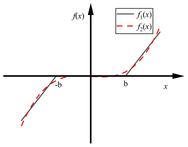
In the above equation, k₀ is average meshing stiffness and k_m is amplitude of fluctuation in meshing stiffness. f(x) represents the function of gear backlash, which can be expressed in a piecewise form as follows:

$$\begin{array}{}\text{(4)}& f_{\mathrm{1}}\left(x\right)=\left\{\begin{array}{l}x-b,x>b,\\ \mathrm{0},-b\le x\le b,\\ x+b,x<-b.\end{array}\right.\end{array}$$

To obtain an analytical solution for the dynamics equation, the function of gear backlash can be simplified to a cubic polynomial form as shown in Eq. (5), and its fitting curve is shown in Fig. 2.

$$\begin{array}{}\text{(5)}& f_{\mathrm{2}}\left(x\right)={\mathit{\gamma }}_{\mathrm{1}}x+{\mathit{\gamma }}_{\mathrm{2}}{x}^{\mathrm{3}}\end{array}$$

In the above equation, γ₁ and γ₂ represent the fitting coefficient of the backlash function.

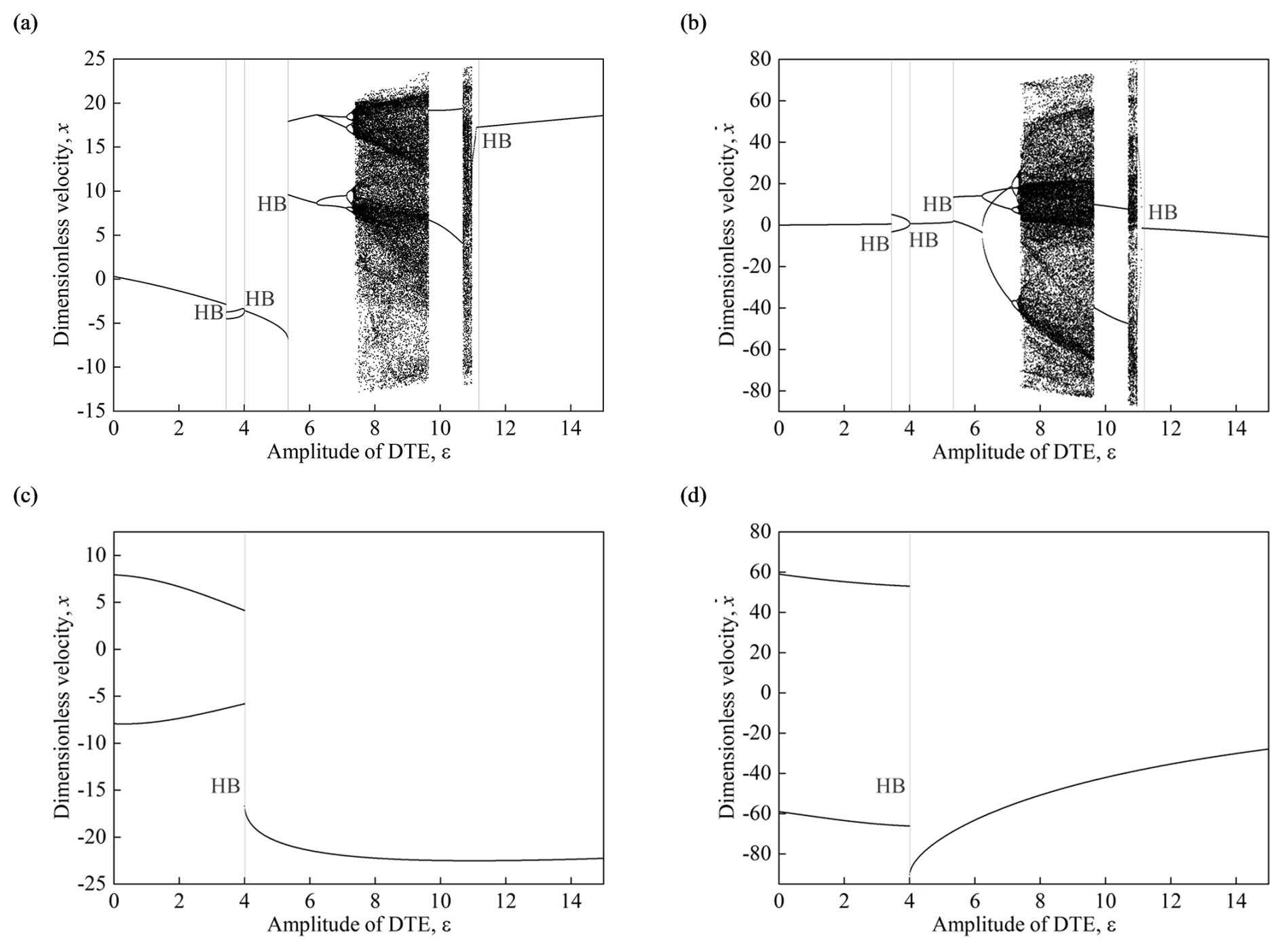
Figure 3 Bifurcation diagrams. (a) x−ε, forward change; (b) $\dot{x}-\mathit{\epsilon }$, forward change; (c) x−ε, reverse change; (d) $\dot{x}-\mathit{\epsilon }$, reverse change. (Ω=2, α= 0.1, β₁= 1, β₂= 0.7, γ₁= 0.3444, γ₂= 0.03004, Q= 0.1, ε∈[0, 15].)

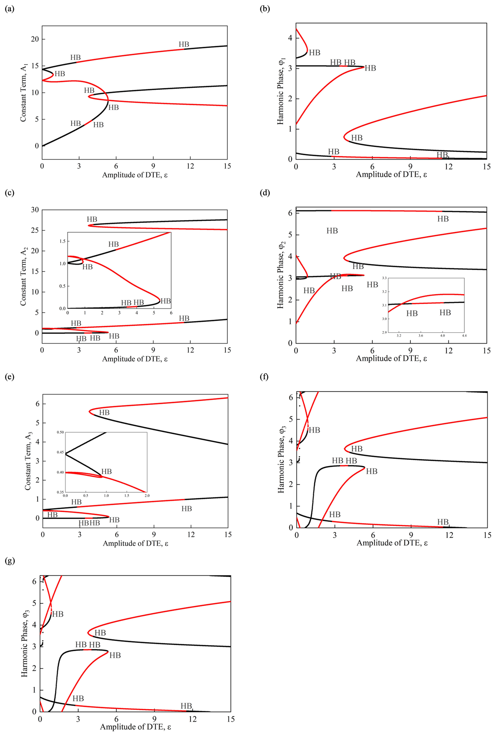
Figure 4 The harmonic amplitude versus the amplitude of DTE for periodic motions in the gear nonlinear dynamic system based on HB3: (a) A₁, (b) φ₁, (c) A₂, (d) φ₂, (e) A₃, (f) φ₃, (g) a₀ (Ω=2, α= 0.1, β₁= 1, β₂= 0.7, γ₁= 0.3444, γ₂=  0.03004, Q= 0.1, εϵ [0, 15]).

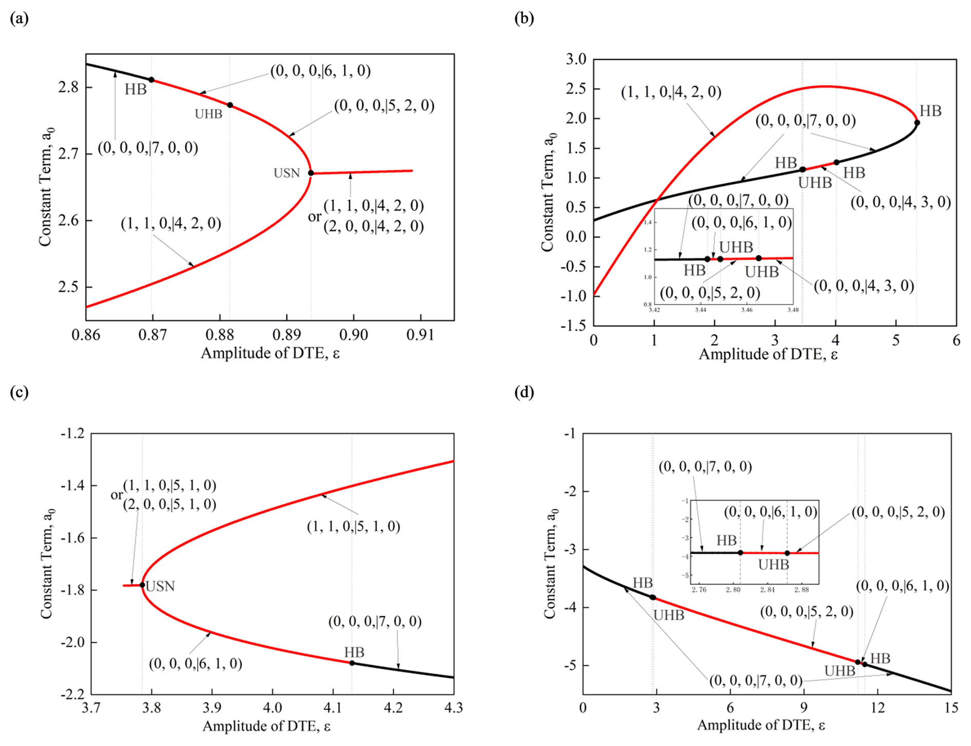
Figure 5 The eigenvalue structures and bifurcation of periodic motions in the gear nonlinear dynamic system based on HB3. (a)–(d) The first, second, third, and fourth branches of periodic motion, a₀, for example (Ω=2, α= 0.1, β₁= 1, β₂= 0.7, γ₁= 0.3444, γ₂= 0.03004, Q=  0.1).

Table 1 The stability of period-1 motion based on HB3.

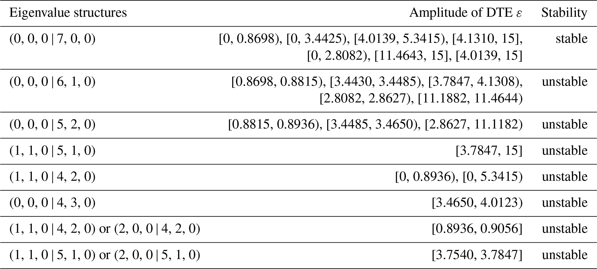
Table 2 The bifurcation points of period-1 motion based on HB3.

3 Analytical solutions

The above dynamical model of gear meshing system can be simplified to the following form through nondimensionalization:

$$\begin{array}{}\text{(6)}& \begin{array}{rl}& \ddot{x}+\mathit{\alpha }\dot{x}+\left({\mathit{\beta }}_{\mathrm{1}}+{\mathit{\beta }}_{\mathrm{2}}\cos \left(\mathrm{\Omega }t\right)\right)\left({\mathit{\gamma }}_{\mathrm{1}}x+{\mathit{\gamma }}_{\mathrm{2}}{x}^{\mathrm{3}}\right)=\\ & Q+Q_{\mathrm{m}}\cos \left(\mathrm{\Omega }t\right).\end{array}\end{array}$$

In this case, the gear discontinuity dynamics equation is transformed into a continuous dynamics equation, which can be solved using the generalized harmonic balance method for continuous dynamical systems. The above equation can be written in standard form as

$$\begin{array}{}\text{(7)}& \ddot{x}=f(\dot{x},x,t),\end{array}$$

where

$$\begin{array}{}\text{(8)}& \begin{array}{rl}& f(\dot{x},x,t)=-\mathit{\alpha }\dot{x}-\left({\mathit{\beta }}_{\mathrm{1}}+{\mathit{\beta }}_{\mathrm{2}}\cos \left(\mathrm{\Omega }t\right)\right)\left({\mathit{\gamma }}_{\mathrm{1}}x+{\mathit{\gamma }}_{\mathrm{2}}{x}^{\mathrm{3}}\right)\\ & +Q+Q_m\cos \left(\mathrm{\Omega }t\right).\end{array}\end{array}$$

Assuming that the continuous dynamical system has a period-m solution with $T=\mathrm{2}\mathit{\pi }/\mathrm{\Omega }$, the analytical expression of the periodic solution can be represented by a Fourier series:

$$\begin{array}{}\text{(9)}& \begin{array}{rl}& x^{\ast }\left(t\right)=a_{\mathrm{0}}^{\left(m\right)}\left(t\right)+\sum _{k=\mathrm{1}}^N\\ & \left[b_{k/m}^{\left(m\right)}\left(t\right)\cos \left({\displaystyle \frac{k}{m}}\mathrm{\Omega }t\right)+c_{k/m}^{\left(m\right)}\left(t\right)\sin \left({\displaystyle \frac{k}{m}}\mathrm{\Omega }t\right)\right].\end{array}\end{array}$$

The first and second derivatives of the periodic solution are as follows:

$$\begin{array}{}\text{(10)}& \begin{array}{l}{\dot{x}}^{\ast }\left(t\right)={\dot{a}}_{\mathrm{0}}^{\left(m\right)}\left(t\right)+\sum _{k=\mathrm{1}}^N\left[\left({\dot{b}}_{k/m}^{\left(m\right)}\left(t\right)+\frac{k\mathrm{\Omega }}{m}{c}_{k/m}^{\left(m\right)}\left(t\right)\right)\cos \right.\\ \left.\left(\frac{k\mathrm{\Omega }}{m}t\right)+\left({\dot{c}}_{k/m}^{\left(m\right)}\left(t\right)-\frac{k\mathrm{\Omega }}{m}{b}_{k/m}^{\left(m\right)}\left(t\right)\right)\sin \left(\frac{k\mathrm{\Omega }}{m}t\right)\right],\end{array}\end{array}$$

$$\begin{array}{}\text{(11)}& \begin{array}{l}{\ddot{x}}^{\ast }\left(t\right)={\ddot{a}}_{\mathrm{0}}^{\left(m\right)}\left(t\right)+\sum _{k=\mathrm{1}}^N\left[\left({\ddot{b}}_{k/m}^{\left(m\right)}\left(t\right)+\mathrm{2}\frac{k\mathrm{\Omega }}{m}{\dot{c}}_{k/m}^{\left(m\right)}\left(t\right)\right.\right.\\ \left.-{\left(\frac{k\mathrm{\Omega }}{m}\right)}^{\mathrm{2}}{b}_{k/m}^{\left(m\right)}\left(t\right)\right)\cos \left(\frac{k\mathrm{\Omega }}{m}t\right)+\left({\ddot{c}}_{k/m}^{\left(m\right)}\left(t\right)-\right.\\ \left.\left.\mathrm{2}\frac{k\mathrm{\Omega }}{m}{\dot{b}}_{k/m}^{\left(m\right)}\left(t\right)-{\left(\frac{k\mathrm{\Omega }}{m}\right)}^{\mathrm{2}}{c}_{k/m}^{\left(m\right)}\left(t\right)\right)\sin \left(\frac{k\mathrm{\Omega }}{m}t\right)\right].\end{array}\end{array}$$

By substituting Eqs. (9)–(11) into Eq. (6) and balancing the coefficients of each harmonic component cos($k\mathrm{\Omega }t/m$) and sin($k\mathrm{\Omega }t/m$) (k=1, 2, ..., N), the original dynamic system can be transformed into a new dynamic system for calculating the Fourier series coefficients:

$$\begin{array}{}\text{(12)}& \left\{\begin{array}{l}{\ddot{a}}_{\mathrm{0}}^{\left(m\right)}=F_{\mathrm{0}}\left(a_{\mathrm{0}}^{\left(m\right)},{\mathit{b}}^{\left(m\right)},{\mathit{c}}^{\left(m\right)},{\dot{a}}_{\mathrm{0}}^{\left(m\right)},{\dot{\mathit{b}}}^{\left(m\right)},{\dot{\mathit{c}}}^{\left(m\right)}\right),\\ {\ddot{\mathit{b}}}^{\left(m\right)}=-\mathrm{2}\frac{\mathrm{\Omega }}{m}{\mathit{k}}_{\mathrm{1}}{\dot{\mathit{c}}}^{\left(m\right)}+(\frac{\mathrm{\Omega }}{m}{)}^{\mathrm{2}}{\mathit{k}}_{\mathrm{2}}{\mathit{b}}^{\left(m\right)}+{\mathit{F}}_{\mathrm{1}}\\ \left(a_{\mathrm{0}}^{\left(m\right)},{\mathit{b}}^{\left(m\right)},{\mathit{c}}^{\left(m\right)},{\dot{a}}_{\mathrm{0}}^{\left(m\right)},{\dot{\mathit{b}}}^{\left(m\right)},{\dot{\mathit{c}}}^{\left(m\right)}\right),\\ {\ddot{\mathit{c}}}^{\left(m\right)}=\mathrm{2}\frac{\mathrm{\Omega }}{m}{\mathit{k}}_{\mathrm{1}}{\dot{\mathit{b}}}^{\left(m\right)}+(\frac{\mathrm{\Omega }}{m}{)}^{\mathrm{2}}{\mathit{k}}_{\mathrm{2}}{\mathit{c}}^{\left(m\right)}+{\mathit{F}}_{\mathrm{2}}\\ \left(a_{\mathrm{0}}^{\left(m\right)},{\mathit{b}}^{\left(m\right)},{\mathit{c}}^{\left(m\right)},{\dot{a}}_{\mathrm{0}}^{\left(m\right)},{\dot{\mathit{b}}}^{\left(m\right)},{\dot{\mathit{c}}}^{\left(m\right)}\right),\end{array}\right.\end{array}$$

where

$$\begin{array}{}\text{(13)}& \begin{array}{l}{\mathit{k}}_{\mathrm{1}}=\mathrm{diag}[\mathrm{1},\mathrm{2},\mathrm{\dots },N],\\ {\mathit{k}}_{\mathrm{2}}=\mathrm{diag}[\mathrm{1},{\mathrm{2}}^{\mathrm{2}},\mathrm{\dots },N^{\mathrm{2}}],\\ {\mathit{b}}^{\left(m\right)}={\left(b_{\mathrm{1}/m}^{\left(m\right)},b_{\mathrm{2}/m}^{\left(m\right)},\mathrm{\dots },b_{N/m}^{\left(m\right)}\right)}^T,\\ {\mathit{c}}^{\left(m\right)}={\left(c_{\mathrm{1}/m}^{\left(m\right)},c_{\mathrm{2}/m}^{\left(m\right)},\mathrm{\dots },c_{N/m}^{\left(m\right)}\right)}^T,\\ {\mathit{F}}_{\mathrm{1}}={\left(F_{\mathrm{11}},F_{\mathrm{12}},\mathrm{\dots },F_{\mathrm{1}N}\right)}^T,\\ {\mathit{F}}_{\mathrm{2}}={\left(F_{\mathrm{21}},F_{\mathrm{22}},\mathrm{\dots },F_{\mathrm{2}N}\right)}^T,\end{array}\end{array}$$

and

$$\begin{array}{}\text{(14)}& \begin{array}{l}{F}_{\mathrm{0}}\left(a_{\mathrm{0}}^{\left(m\right)},{\mathit{b}}^{\left(m\right)},{\mathit{c}}^{\left(m\right)},{\dot{a}}_{\mathrm{0}}^{\left(m\right)},{\dot{\mathit{b}}}^{\left(m\right)},{\dot{\mathit{c}}}^{\left(m\right)}\right)\\ =\frac{\mathrm{1}}{mT}\underset{\mathrm{0}}{\overset{mT}{\int }}f(\dot{x},x,t)\mathrm{d}t,\\ F_{\mathrm{1}k}\left(a_{\mathrm{0}}^{\left(m\right)},{\mathit{b}}^{\left(m\right)},{\mathit{c}}^{\left(m\right)},{\dot{a}}_{\mathrm{0}}^{\left(m\right)},{\dot{\mathit{b}}}^{\left(m\right)},{\dot{\mathit{c}}}^{\left(m\right)}\right)\\ =\frac{\mathrm{2}}{mT}\underset{\mathrm{0}}{\overset{mT}{\int }}f(\dot{x},x,t)\cos \left(\frac{k\mathrm{\Omega }}{m}t\right)\mathrm{d}t,\\ F_{\mathrm{2}k}\left(a_{\mathrm{0}}^{\left(m\right)},{\mathit{b}}^{\left(m\right)},{\mathit{c}}^{\left(m\right)},{\dot{a}}_{\mathrm{0}}^{\left(m\right)},{\dot{\mathit{b}}}^{\left(m\right)},{\dot{\mathit{c}}}^{\left(m\right)}\right)\\ =\frac{\mathrm{2}}{mT}\underset{\mathrm{0}}{\overset{mT}{\int }}f(\dot{x},x,t)\sin \left(\frac{k\mathrm{\Omega }}{m}t\right)\mathrm{d}t,\\ k=\mathrm{1},\mathrm{2},\mathrm{\dots },N.\end{array}\end{array}$$

The following equations can be obtained by calculation:

$$\begin{array}{}\text{(15)}& \begin{array}{l}{F}_{\mathrm{0}}\left(a_{\mathrm{0}}^{\left(m\right)},{\mathit{b}}^{\left(m\right)},{\mathit{c}}^{\left(m\right)},{\dot{a}}_{\mathrm{0}}^{\left(m\right)},{\dot{\mathit{b}}}^{\left(m\right)},{\dot{\mathit{c}}}^{\left(m\right)}\right)\\ =-\mathit{\alpha }{\dot{a}}_{\mathrm{0}}^{\left(m\right)}-{\mathit{\beta }}_{\mathrm{1}}{\mathit{\gamma }}_{\mathrm{1}}{a}_{\mathrm{0}}^{\left(m\right)}-{\mathit{\beta }}_{\mathrm{1}}{\mathit{\gamma }}_{\mathrm{2}}{f}_{\mathrm{1}}\\ -\frac{\mathrm{1}}{\mathrm{2}}{\mathit{\beta }}_{\mathrm{2}}{\mathit{\gamma }}_{\mathrm{1}}{b}_{m/m}^{\left(m\right)}-{\mathit{\beta }}_{\mathrm{2}}{\mathit{\gamma }}_{\mathrm{2}}{f}_{\mathrm{2}}-Q_m,\\ F_{\mathrm{1}k}\left(a_{\mathrm{0}}^{\left(m\right)},{\mathit{b}}^{\left(m\right)},{\mathit{c}}^{\left(m\right)},{\dot{a}}_{\mathrm{0}}^{\left(m\right)},{\dot{\mathit{b}}}^{\left(m\right)},{\dot{\mathit{c}}}^{\left(m\right)}\right)\\ =-\mathit{\alpha }({\dot{b}}_{k/m}^{\left(m\right)}+\frac{k\mathrm{\Omega }}{m}{c}_{k/m}^{\left(m\right)})-{\mathit{\beta }}_{\mathrm{1}}{\mathit{\gamma }}_{\mathrm{1}}{b}_{k/m}^{\left(m\right)}\\ -{\mathit{\beta }}_{\mathrm{2}}{\mathit{\gamma }}_{\mathrm{1}}{f}_{\mathrm{3}k}-{\mathit{\beta }}_{\mathrm{2}}{\mathit{\gamma }}_{\mathrm{2}}{f}_{\mathrm{4}k}-{\mathit{\beta }}_{\mathrm{1}}{\mathit{\gamma }}_{\mathrm{2}}{f}_{\mathrm{7}k}+Q_m{\mathit{\delta }}_k^m,\\ F_{\mathrm{2}k}\left(a_{\mathrm{0}}^{\left(m\right)},{\mathit{b}}^{\left(m\right)},{\mathit{c}}^{\left(m\right)},{\dot{a}}_{\mathrm{0}}^{\left(m\right)},{\dot{\mathit{b}}}^{\left(m\right)},{\dot{\mathit{c}}}^{\left(m\right)}\right)\\ =-\mathit{\alpha }({\dot{c}}_{k/m}^{\left(m\right)}-\frac{k\mathrm{\Omega }}{m}{b}_{k/m}^{\left(m\right)})-{\mathit{\beta }}_{\mathrm{1}}{\mathit{\gamma }}_{\mathrm{1}}{c}_{k/m}^{\left(m\right)}\\ -{\mathit{\beta }}_{\mathrm{2}}{\mathit{\gamma }}_{\mathrm{1}}{f}_{\mathrm{5}k}-{\mathit{\beta }}_{\mathrm{2}}{\mathit{\gamma }}_{\mathrm{2}}{f}_{\mathrm{6}k}-{\mathit{\beta }}_{\mathrm{1}}{\mathit{\gamma }}_{\mathrm{2}}{f}_{\mathrm{8}k},\\ k=\mathrm{1},\mathrm{2},\mathrm{\dots },N,\end{array}\end{array}$$

where

$$\begin{array}{}\text{(16)}& \begin{array}{l}{f}_{\mathrm{1}}=\frac{\mathrm{1}}{mT}\underset{\mathrm{0}}{\overset{mT}{\int }}{x}^{\mathrm{3}}\mathrm{d}t\\ =(a_{\mathrm{0}}^{\left(m\right)}{)}^{\mathrm{3}}+\mathrm{3}{a}_{\mathrm{0}}^{\left(m\right)}\sum _{i=\mathrm{1}}^N\sum _{j=\mathrm{1}}^N{b}_{i/m}^{\left(m\right)}{b}_{j/m}^{\left(m\right)}{f}_{\mathrm{20}}(i,j)\\ +c_{i/m}^{\left(m\right)}{c}_{j/m}^{\left(m\right)}{f}_{\mathrm{22}}(i,j)\\ +\sum _{i=\mathrm{1}}^N\sum _{j=\mathrm{1}}^N\sum _{l=\mathrm{1}}^N\left[b_{i/m}^{\left(m\right)}{b}_{j/m}^{\left(m\right)}{b}_{l/m}^{\left(m\right)}{f}_{\mathrm{30}}\right(i,j,l)\\ +\mathrm{3}{b}_{i/m}^{\left(m\right)}{c}_{j/m}^{\left(m\right)}{c}_{l/m}^{\left(m\right)}{f}_{\mathrm{32}}(l,j,i)],\end{array}\end{array}$$

$$\begin{array}{}\text{(17)}& \begin{array}{l}{f}_{\mathrm{2}}=\frac{\mathrm{1}}{mT}\underset{\mathrm{0}}{\overset{mT}{\int }}{x}^{\mathrm{3}}\cos \left(\mathrm{\Omega }t\right)\mathrm{d}t\\ =\mathrm{3}\left(a_{\mathrm{0}}^{\left(m\right)}{)}^{\mathrm{2}}\sum _{i=\mathrm{1}}^N{b}_{i/m}^{\left(m\right)}{f}_{\mathrm{20}}\right(i,m)+\mathrm{3}{a}_{\mathrm{0}}^{\left(m\right)}\sum _{i=\mathrm{1}}^N\sum _{j=\mathrm{1}}^N\\ \left[b_{i/m}^{\left(m\right)}{b}_{j/m}^{\left(m\right)}{f}_{\mathrm{30}}(i,j,m)+c_{i/m}^{\left(m\right)}{c}_{j/m}^{\left(m\right)}{f}_{\mathrm{32}}(i,j,m)\right]\\ +\sum _{i=\mathrm{1}}^N\sum _{j=\mathrm{1}}^N\sum _{l=\mathrm{1}}^N\left[b_{i/m}^{\left(m\right)}{b}_{j/m}^{\left(m\right)}{b}_{l/m}^{\left(m\right)}{f}_{\mathrm{40}}(i,j,l,m)\right.\\ \left.+\mathrm{3}{c}_{i/m}^{\left(m\right)}{c}_{j/m}^{\left(m\right)}{b}_{l/m}^{\left(m\right)}{f}_{\mathrm{42}}(i,j,l,m)\right],\end{array}\end{array}$$

$$\begin{array}{}\text{(18)}& \begin{array}{rl}& f_{\mathrm{3}k}={\displaystyle \frac{\mathrm{2}}{mT}}\underset{\mathrm{0}}{\overset{mT}{\int }}x\cos \left(\mathrm{\Omega }t\right)\cos \left({\displaystyle \frac{k\mathrm{\Omega }}{m}}t\right)\mathrm{d}t\\ & =\mathrm{2}{a}_{\mathrm{0}}^{\left(m\right)}{f}_{\mathrm{20}}(m,k)+\mathrm{2}\sum _{i=\mathrm{1}}^N{b}_{i/m}^{\left(m\right)}{f}_{\mathrm{30}}(i,m,k),\end{array}\end{array}$$

$$\begin{array}{}\text{(19)}& \begin{array}{l}{f}_{\mathrm{4}k}=\frac{\mathrm{2}}{mT}\underset{\mathrm{0}}{\overset{mT}{\int }}{x}^{\mathrm{3}}\cos \left(\mathrm{\Omega }t\right)\cos \left(\frac{k\mathrm{\Omega }}{m}t\right)\mathrm{d}t\\ =\mathrm{2}\left(a_{\mathrm{0}}^{\left(m\right)}{)}^{\mathrm{3}}{f}_{\mathrm{20}}\right(m,k)+\mathrm{6}(a_{\mathrm{0}}^{\left(m\right)}{)}^{\mathrm{2}}\sum _{i=\mathrm{1}}^N{b}_{i/m}^{\left(m\right)}{f}_{\mathrm{33}}(i,m,k)\\ +\mathrm{6}{a}_{\mathrm{0}}^{\left(m\right)}\sum _{i=\mathrm{1}}^N\sum _{j=\mathrm{1}}^N\left[b_{i/m}^{\left(m\right)}{b}_{j/m}^{\left(m\right)}{f}_{\mathrm{40}}\right(i,j,m,k)\\ +c_{i/m}^{\left(m\right)}{c}_{j/m}^{\left(m\right)}{f}_{\mathrm{42}}(i,j,m,k)]\\ +\mathrm{2}\sum _{i=\mathrm{1}}^N\sum _{j=\mathrm{1}}^N\sum _{l=\mathrm{1}}^N\left[\mathrm{3}{c}_{i/m}^{\left(m\right)}{c}_{j/m}^{\left(m\right)}{b}_{l/m}^{\left(m\right)}{f}_{\mathrm{52}}\right(i,j,l,m,k)\\ +b_{i/m}^{\left(m\right)}{b}_{j/m}^{\left(m\right)}{b}_{l/m}^{\left(m\right)}{f}_{\mathrm{50}}(i,j,l,m,k)],\end{array}\end{array}$$

$$\begin{array}{}\text{(20)}& \begin{array}{l}{f}_{\mathrm{5}k}=\frac{\mathrm{2}}{mT}\underset{\mathrm{0}}{\overset{mT}{\int }}x\cos \left(\mathrm{\Omega }t\right)\sin \left(\frac{k\mathrm{\Omega }}{m}t\right)\mathrm{d}t\\ =\mathrm{2}\sum _{i=\mathrm{1}}^N{c}_{i/m}^{\left(m\right)}{f}_{\mathrm{32}}(i,k,m),\end{array}\end{array}$$

$$\begin{array}{}\text{(21)}& \begin{array}{l}{f}_{\mathrm{6}k}=\frac{\mathrm{2}}{mT}\underset{\mathrm{0}}{\overset{mT}{\int }}{x}^{\mathrm{3}}\cos \left(\mathrm{\Omega }t\right)\sin \left(\frac{k\mathrm{\Omega }}{m}t\right)\mathrm{d}t\\ =\mathrm{6}\left(a_{\mathrm{0}}^{\left(m\right)}{)}^{\mathrm{2}}\sum _{i=\mathrm{1}}^N{c}_{i/m}^{\left(m\right)}{f}_{\mathrm{32}}\right(i,k,m)\\ +\mathrm{12}{a}_{\mathrm{0}}^{\left(m\right)}\sum _{i=\mathrm{1}}^N\sum _{j=\mathrm{1}}^N{b}_{i/m}^{\left(m\right)}{c}_{j/m}^{\left(m\right)}{f}_{\mathrm{42}}(j,k,m,i)\\ +\mathrm{2}\sum _{i=\mathrm{1}}^N\sum _{j=\mathrm{1}}^N\sum _{l=\mathrm{1}}^N\left[c_{i/m}^{\left(m\right)}{c}_{j/m}^{\left(m\right)}{c}_{l/m}^{\left(m\right)}{f}_{\mathrm{54}}(i,j,l,k,m)\right.\\ \left.+\mathrm{3}{c}_{i/m}^{\left(m\right)}{b}_{j/m}^{\left(m\right)}{b}_{l/m}^{\left(m\right)}{f}_{\mathrm{52}}(i,k,m,j,l)\right],\end{array}\end{array}$$

$$\begin{array}{}\text{(22)}& \begin{array}{l}{f}_{\mathrm{7}k}=\frac{\mathrm{2}}{mT}\underset{\mathrm{0}}{\overset{mT}{\int }}{x}^{\mathrm{3}}\sin \left(\frac{k\mathrm{\Omega }}{m}t\right)\mathrm{d}t\\ =\mathrm{6}\left(a_{\mathrm{0}}^{\left(m\right)}{)}^{\mathrm{2}}\sum _{i=\mathrm{1}}^N{b}_{i/m}^{\left(m\right)}{f}_{\mathrm{20}}\right(i,k)\\ +\mathrm{6}{a}_{\mathrm{0}}^{\left(m\right)}\sum _{i=\mathrm{1}}^N\sum _{j=\mathrm{1}}^N{b}_{i/m}^{\left(m\right)}{b}_{j/m}^{\left(m\right)}{f}_{\mathrm{30}}(i,j,k)+c_{i/m}^{\left(m\right)}{c}_{j/m}^{\left(m\right)}\\ f_{\mathrm{32}}(i,j,k)+\mathrm{2}\sum _{i=\mathrm{1}}^N\sum _{j=\mathrm{1}}^N\sum _{l=\mathrm{1}}^N\left[b_{i/m}^{\left(m\right)}{b}_{j/m}^{\left(m\right)}{b}_{l/m}^{\left(m\right)}{f}_{\mathrm{40}}(i,j,l,k)\right.\\ \left.+\mathrm{3}{c}_{i/m}^{\left(m\right)}{c}_{j/m}^{\left(m\right)}{b}_{l/m}^{\left(m\right)}{f}_{\mathrm{42}}(i,j,l,k)\right],\end{array}\end{array}$$

$$\begin{array}{}\text{(23)}& \begin{array}{l}{f}_{\mathrm{8}k}=\frac{\mathrm{2}}{mT}\underset{\mathrm{0}}{\overset{mT}{\int }}{x}^{\mathrm{3}}\cos \left(\frac{k\mathrm{\Omega }}{m}t\right)\mathrm{d}t\\ =\mathrm{6}\left(a_{\mathrm{0}}^{\left(m\right)}{)}^{\mathrm{2}}\sum _{i=\mathrm{1}}^N{c}_{i/m}^{\left(m\right)}{f}_{\mathrm{22}}\right(i,k)\\ +\mathrm{12}{a}_{\mathrm{0}}^{\left(m\right)}\sum _{i=\mathrm{1}}^N\sum _{j=\mathrm{1}}^N{c}_{i/m}^{\left(m\right)}{b}_{j/m}^{\left(m\right)}{f}_{\mathrm{32}}(i,k,j)\\ +\mathrm{2}\sum _{i=\mathrm{1}}^N\sum _{j=\mathrm{1}}^N\sum _{l=\mathrm{1}}^N\left[\mathrm{3}{c}_{i/m}^{\left(m\right)}{b}_{j/m}^{\left(m\right)}{b}_{l/m}^{\left(m\right)}{f}_{\mathrm{42}}(i,k,j,l)\right.\\ \left.+c_{i/m}^{\left(m\right)}{c}_{j/m}^{\left(m\right)}{c}_{l/m}^{\left(m\right)}{f}_{\mathrm{44}}(i,j,l,k)\right],\end{array}\end{array}$$

and

$$\begin{array}{l}{\displaystyle }{f}_{\mathrm{20}}(i,j)=({\mathit{\delta }}_{i-j}^{\mathrm{0}}+{\mathit{\delta }}_{i+j}^{\mathrm{0}})/\mathrm{2},\\ {\displaystyle }{f}_{\mathrm{22}}(i,j)=({\mathit{\delta }}_{i-j}^{\mathrm{0}}-{\mathit{\delta }}_{i+j}^{\mathrm{0}})/\mathrm{2},\end{array}$$

$$\begin{array}{}\text{(24)}& {\displaystyle }{f}_{\mathrm{30}}(i,j,l)=({\mathit{\delta }}_{i-j+l}^{\mathrm{0}}+{\mathit{\delta }}_{i+j-l}^{\mathrm{0}}+{\mathit{\delta }}_{i-j-l}^{\mathrm{0}}+{\mathit{\delta }}_{i+j+l}^{\mathrm{0}})/\mathrm{4},\text{(25)}& {\displaystyle }{f}_{\mathrm{32}}(i,j,l)=({\mathit{\delta }}_{i-j+l}^{\mathrm{0}}+{\mathit{\delta }}_{i-j-l}^{\mathrm{0}}-{\mathit{\delta }}_{i+j-l}^{\mathrm{0}}-{\mathit{\delta }}_{i+j+l}^{\mathrm{0}})/\mathrm{4},\text{(26)}& {\displaystyle }{f}_{\mathrm{40}}(i,j,l,k)=({\mathit{\delta }}_{i+j+l}^k+{\mathit{\delta }}_{\left|i+j-l\right|}^k+{\mathit{\delta }}_{\left|i-j+l\right|}^k+{\mathit{\delta }}_{\left|i-j-l\right|}^k)/\mathrm{8},\text{(27)}& {\displaystyle }{f}_{\mathrm{42}}(i,j,l,k)=({\mathit{\delta }}_{\left|i-j+l\right|}^k+{\mathit{\delta }}_{\left|i-j-l\right|}^k-{\mathit{\delta }}_{\left|i+j+l\right|}^k-{\mathit{\delta }}_{\left|i+j-l\right|}^k)/\mathrm{8},\text{(28)}& {\displaystyle }\begin{array}{l}{f}_{\mathrm{44}}(i,j,l,k)=(-{\mathit{\delta }}_{i+j+l}^k+\mathrm{sign}(i+j-l){\mathit{\delta }}_{\left|i+j-l\right|}^k\\ +\mathrm{sign}(i-j+l){\mathit{\delta }}_{\left|i-j+l\right|}^k-\mathrm{sign}(i-j-l){\mathit{\delta }}_{\left|i-j-l\right|}^k)/\mathrm{8},\end{array}\text{(29)}& {\displaystyle }\begin{array}{l}{f}_{\mathrm{50}}(i,j,l,k,m)=({\mathit{\delta }}_{i+j+l}^{k+m}+{\mathit{\delta }}_{\left|i+j-l\right|}^{k+m}+{\mathit{\delta }}_{\left|i-j+l\right|}^{k+m}+{\mathit{\delta }}_{\left|i-j-l\right|}^{k+m}\\ +{\mathit{\delta }}_{i+j+l}^{k-m}+{\mathit{\delta }}_{\left|i+j-l\right|}^{k-m}+{\mathit{\delta }}_{\left|i-j+l\right|}^{k-m}+{\mathit{\delta }}_{\left|i-j-l\right|}^{k-m})/\mathrm{16},\end{array}\text{(30)}& {\displaystyle }\begin{array}{l}{f}_{\mathrm{52}}(i,j,l,k,m)=({\mathit{\delta }}_{\left|i-j+l\right|}^{k+m}+{\mathit{\delta }}_{\left|i-j-l\right|}^{k+m}-{\mathit{\delta }}_{i+j+l}^{k+m}-{\mathit{\delta }}_{\left|i+j-l\right|}^{k+m}\\ +{\mathit{\delta }}_{\left|i-j+l\right|}^{k-m}+{\mathit{\delta }}_{\left|i-j-l\right|}^{k-m}-{\mathit{\delta }}_{i+j+l}^{k-m}-{\mathit{\delta }}_{\left|i+j-l\right|}^{k-m})/\mathrm{16},\end{array}\text{(31)}& {\displaystyle }\begin{array}{l}{f}_{\mathrm{54}}(i,j,l,k,m)=(-{\mathit{\delta }}_{i+j+l}^{k+m}+\mathrm{sign}(i-j+l){\mathit{\delta }}_{\left|i-j+l\right|}^{k+m}\\ +\mathrm{sign}(i+j-l){\mathit{\delta }}_{\left|i+j-l\right|}^{k+m}+\mathrm{sign}(-i+j+l){\mathit{\delta }}_{\left|-i+j+l\right|}^{k+m}\\ -{\mathit{\delta }}_{i+j+l}^{k-m}+\mathrm{sign}(i-j+l){\mathit{\delta }}_{\left|i-j+l\right|}^{k-m}+\mathrm{sign}\\ (i+j-l){\mathit{\delta }}_{\left|i+j-l\right|}^{k-m}+\mathrm{sign}(-i+j+l){\mathit{\delta }}_{\left|-i+j+l\right|}^{k-m})/\mathrm{16},\end{array}\end{array}$$

and finally

$$\begin{array}{}\text{(32)}& {\mathit{\delta }}_j^i=\left\{\begin{array}{l}\mathrm{0},i\ne j,\\ \mathrm{1},i=j,\end{array}\right.\mathrm{sign}=\left\{\begin{array}{l}\mathrm{1},i>\mathrm{0},\\ \mathrm{0},i=\mathrm{0},\\ -\mathrm{1},i<\mathrm{0}.\end{array}\right.\end{array}$$

Define

$$\begin{array}{}\text{(33)}& \begin{array}{l}{\mathit{z}}^{\left(m\right)}=(a_{\mathrm{0}}^{\left(m\right)},{\mathit{b}}^{\left(m\right)},{\mathit{c}}^{\left(m\right)}{)}^{\mathrm{T}}\\ =(a_{\mathrm{0}}^{\left(m\right)},b_{\mathrm{1}/m}^{\left(m\right)},\mathrm{\dots },b_{N/m}^{\left(m\right)},c_{\mathrm{1}/m}^{\left(m\right)},\mathrm{\dots },c_{N/m}^{\left(m\right)}{)}^{\mathrm{T}},\\ {\mathit{z}}_{\mathrm{1}}^{\left(m\right)}={\dot{\mathit{z}}}^{\left(m\right)}=({\dot{a}}_{\mathrm{0}}^{\left(m\right)},{\dot{\mathit{b}}}^{\left(m\right)},{\dot{\mathit{c}}}^{\left(m\right)}{)}^{\mathrm{T}}\\ =({\dot{a}}_{\mathrm{0}}^{\left(m\right)},{\dot{b}}_{\mathrm{1}/m}^{\left(m\right)},\mathrm{\dots },{\dot{b}}_{N/m}^{\left(m\right)},{\dot{c}}_{\mathrm{1}/m}^{\left(m\right)},\mathrm{\dots },{\dot{c}}_{N/m}^{\left(m\right)}{)}^{\mathrm{T}}.\end{array}\end{array}$$

The state equation for Eq. (33) is expressed as follows:

$$\begin{array}{}\text{(34)}& \left\{\begin{array}{l}{\dot{\mathit{z}}}^{\left(m\right)}={\mathit{z}}_{\mathrm{1}}^{\left(m\right)},\\ {\dot{\mathit{z}}}_{\mathrm{1}}^{\left(m\right)}={\mathit{g}}^{\left(m\right)}{\left({\mathit{z}}^{\left(m\right)},{\mathit{z}}_{\mathrm{1}}^{\left(m\right)}\right)}^{\mathrm{T}},\end{array}\right.\end{array}$$

where

$$\begin{array}{}\text{(35)}& \begin{array}{rl}& {\mathit{g}}^{\left(m\right)}({\mathit{z}}^{\left(m\right)},{\mathit{z}}_{\mathrm{1}}^{\left(m\right)})\\ & =\left(\begin{array}{l}{F}_{\mathrm{0}}({\mathit{z}}^{\left(m\right)},{\mathit{z}}_{\mathrm{1}}^{\left(m\right)})\\ -\mathrm{2}\frac{\mathrm{\Omega }}{m}{\mathit{k}}_{\mathrm{1}}{\dot{\mathit{c}}}^{\left(m\right)}+(\frac{\mathrm{\Omega }}{m}{)}^{\mathrm{2}}{\mathit{k}}_{\mathrm{2}}{\mathit{b}}^{\left(m\right)}+{\mathit{F}}_{\mathrm{1}}({\mathit{z}}^{\left(m\right)},{\mathit{z}}_{\mathrm{1}}^{\left(m\right)})\\ \mathrm{2}\frac{\mathrm{\Omega }}{m}{\mathit{k}}_{\mathrm{1}}{\dot{\mathit{b}}}^{\left(m\right)}+(\frac{\mathrm{\Omega }}{m}{)}^{\mathrm{2}}{\mathit{k}}_{\mathrm{2}}{\mathit{c}}^{\left(m\right)}+{\mathit{F}}_{\mathrm{2}}({\mathit{z}}^{\left(m\right)},{\mathit{z}}_{\mathrm{1}}^{\left(m\right)})\end{array}\right).\end{array}\end{array}$$

Let

$$\begin{array}{}\text{(36)}& \left\{\begin{array}{l}{\mathit{y}}^{\left(m\right)}\equiv ({\mathit{z}}^{\left(m\right)},{\mathit{z}}_{\mathrm{1}}^{\left(m\right)}),\\ {\mathit{f}}^{\left(m\right)}=({\mathit{z}}_{\mathrm{1}}^{\left(m\right)},{\mathit{g}}^{\left(m\right)}{)}^{\mathrm{T}}.\end{array}\right.\end{array}$$

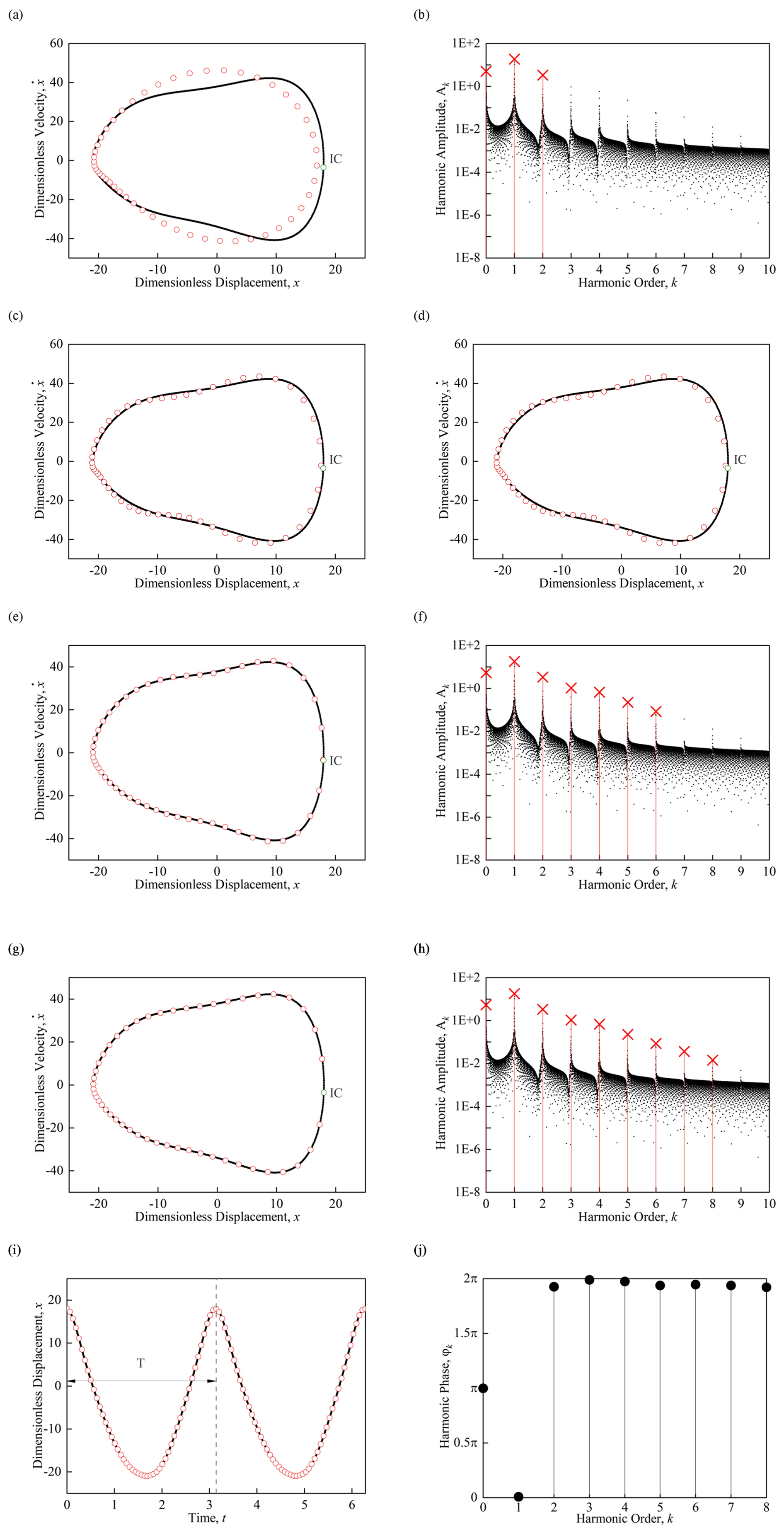
Figure 6 Unstable period-1 motion (ε=  13.26). Panels (a), (c), (e), and (g) show trajectory diagrams compared with numerical solution based on HB2, HB4, HB6, and HB8, respectively. Panels (b), (d), (f), and (h) show amplitude–frequency diagrams compared with numerical solution based on HB2, HB4, HB6, and HB8, respectively. (i) The time histories of displacement diagram based on HB8. (j) The harmonic phase diagram based on HB8 (Ω=2, α=0.1, β₁=1, β₂=0.7, γ₁=0.3444, γ₂=0.03004, Q=0.1; ICs: x≈17.9867, $\dot{x}\approx -\mathrm{3.5406}$, t=0).

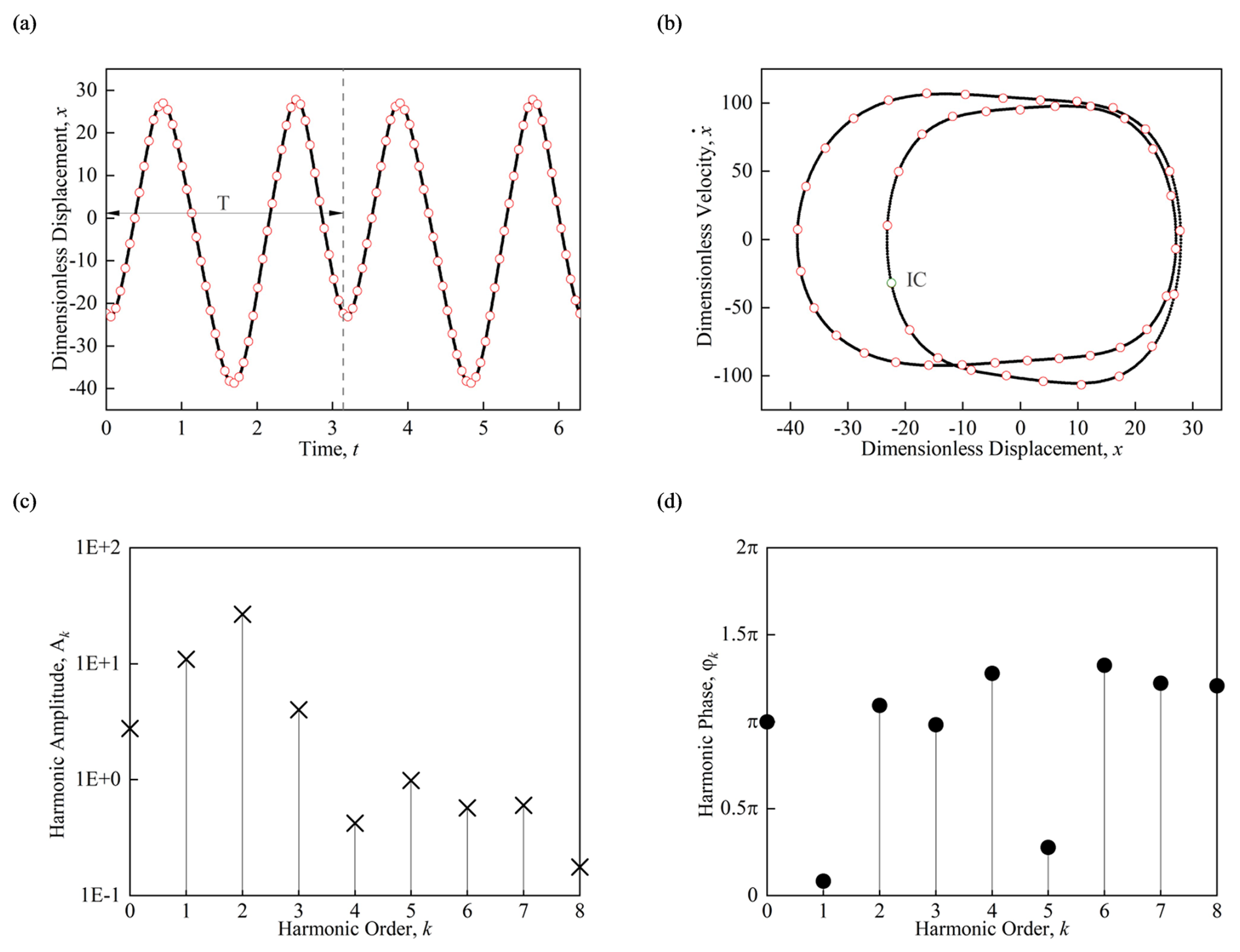
Figure 7 Stable period-1 motion (ε=  13.26). (a) The time histories of displacement diagram, (b) the trajectories diagram, (c) the harmonic amplitude diagram, and (d) the harmonic phase diagram (Ω= 2, α= 0.1, β₁= 1, β₂= 0.7, γ₁= 0.3444, γ₂=0.03004, Q=0.1; ICs: x≈ -22.4261, $\dot{x}\approx$ −31.9578, t= 0).

Therefore, the new dynamic system can be represented as

$$\begin{array}{}\text{(37)}& {\dot{\mathit{y}}}^{\left(m\right)}={\mathit{f}}^{\left(m\right)}\left({\mathit{y}}^{\left(m\right)}\right).\end{array}$$

The steady-state periodic solution of the system can be obtained at ${\dot{y}}^{\left(m\right)}=$ 0, where

$$\begin{array}{}\text{(38)}& \begin{array}{l}{F}_{\mathrm{0}}(a_{\mathrm{0}}^{\left(m\right)},{\mathit{b}}^{\left(m\right)},{\mathit{c}}^{\left(m\right)},\mathrm{0},\mathbf{0},\mathbf{0})=\mathrm{0},\\ {\mathit{F}}_{\mathrm{1}}(a_{\mathrm{0}}^{\left(m\right)},{\mathit{b}}^{\left(m\right)},{\mathit{c}}^{\left(m\right)},\mathrm{0},\mathbf{0},\mathbf{0})+(\frac{\mathrm{\Omega }}{m}{)}^{\mathrm{2}}{\mathit{k}}_{\mathrm{2}}{\mathit{b}}^{\left(m\right)}=\mathbf{0},\\ {\mathit{F}}_{\mathrm{2}}(a_{\mathrm{0}}^{\left(m\right)},{\mathit{b}}^{\left(m\right)},{\mathit{c}}^{\left(m\right)},\mathrm{0},\mathbf{0},\mathbf{0})+(\frac{\mathrm{\Omega }}{m}{)}^{\mathrm{2}}{\mathit{k}}_{\mathrm{2}}{\mathit{c}}^{\left(m\right)}=\mathbf{0}.\end{array}\end{array}$$

The nonlinear system of equations consisting of the above (2N+1) algebraic equations can be solved using the Newton–Raphson method. Assuming that the solution obtained is y^(m)∗ $=(z^{\left(m\right)\ast },\mathrm{0}{)}^T$, the linearized expression of the dynamical system ${\dot{y}}^{\left(m\right)\ast }$ =f^(m) (y^(m)) at the equilibrium point $y^{\left(m\right)\ast }=(z^{\left(m\right)\ast },\mathrm{0}{)}^T$ is

$$\begin{array}{}\text{(39)}& \begin{array}{l}\mathrm{\Delta }{\dot{\mathit{y}}}^{\left(m\right)}=D{\mathit{f}}^{\left(m\right)}\left({\mathit{y}}^{\left(m\right)\ast }\right)\mathrm{\Delta }{\dot{\mathit{y}}}^{\left(m\right)},\\ D{\mathit{f}}^{\left(m\right)}\left({\mathit{y}}^{\left(m\right)\ast }\right)={\left.\frac{\partial {\mathit{f}}^{\left(m\right)}\left({\mathit{y}}^{\left(m\right)}\right)}{\partial {\mathit{y}}^{\left(m\right)}}\right|}_{{\mathit{y}}^{\left(m\right)\ast }}.\end{array}\end{array}$$

The stability of the original nonlinear dynamic system can be analyzed by solving the eigenvalues of the new dynamic system. The eigenvalues of the Jacobian matrix of the new dynamic system can be solved using the following formula:

$$\begin{array}{}\text{(40)}& \begin{array}{rl}& \left|D{\mathit{f}}^{\left(m\right)}\left({\mathit{y}}^{\left(m\right)\ast }\right)-\mathit{\lambda }{\mathit{I}}_{\mathrm{2}(\mathrm{2}N+\mathrm{1})\mathrm{2}(\mathrm{2}N+\mathrm{1})}\right|\\ & =\mathrm{0}\left(n_{\mathrm{1}},n_{\mathrm{2}},n_{\mathrm{3}}\left|n_{\mathrm{4}},n_{\mathrm{5}},n_{\mathrm{6}}\right.\right).\end{array}\end{array}$$

In the above equation, λ_k (k=1, 2, ..., 2N+1) is the eigenvalues of the dynamic system, n₁ represents the number of negative real roots, n₂ represents the number of positive real roots, n₃ represents the number of real roots equal to 0, n₂ represents the number of conjugate complex roots with negative real parts, n₅ represents the number of conjugate complex roots with positive real parts, and n₆ represents the number of conjugate complex roots with real parts equal to 0.

The stability of the system's periodic solution can be determined according to the following criteria:

1. If all the characteristic roots of the system have negative real parts, the periodic solution of the system is stable.

2. If at least one of the characteristic roots of the system has a positive real part, the periodic solution of the system is unstable.

3. The boundary between the stable and unstable equilibrium with higher-order singularity gives the bifurcation conditions and stability with higher-order singularity.

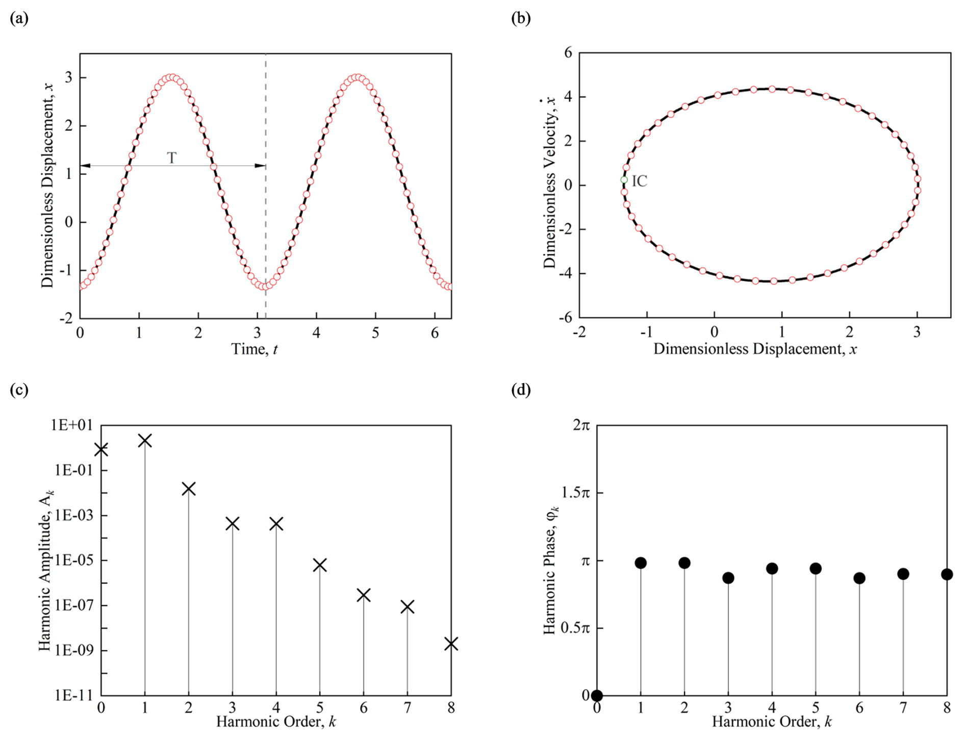
Figure 8 Stable period-1 motion (ε= 2). (a) The time histories of displacement diagram, (b) the trajectories diagram, (c) the harmonic amplitude diagram, and (d) the harmonic phase diagram (Ω= 2, α= 0.1, β₁= 1, β₂= 0.7, γ₁= 0.3444, γ₂= 0.03004, Q=0.1; ICs: x≈ -1.3399, $\dot{x}\approx$ 0.2507, t= 0).

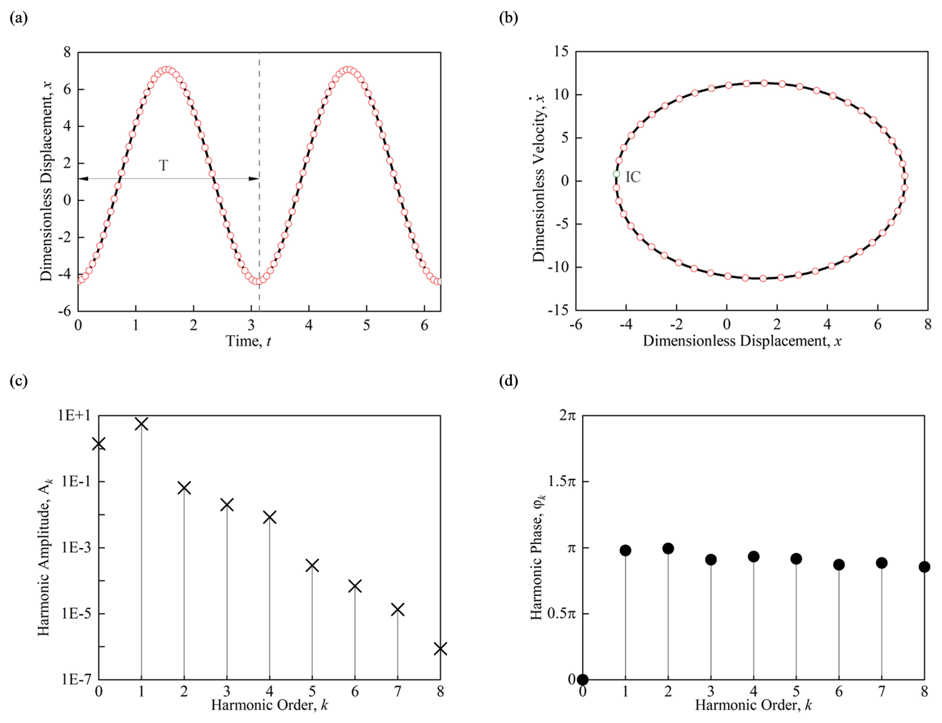
Figure 9 Stable period-1 motion (ε= 4.56). (a) The time histories of displacement diagram, (b) the trajectories diagram, (c) the harmonic amplitude diagram, and (d) the harmonic phase diagram (Ω= 2, α= 0.1, β₁= 1, β₂= 0.7, γ₁= 0.3444, γ₂= 0.03004, Q=0.1; ICs: x≈ -4.3849, $\dot{x}\approx$ 0.8194, and t= 0).

4 Stability and bifurcation analysis

The gear parameters for the gear pair are as follows: the number of teeth for the driving and driven gears is z₁= 30 and z₂= 60, respectively, with a face width of 100 and 95 mm, a module of m=3 mm, and a pressure angle of α₀= 20°. Figure 3 shows the bifurcation diagram of the amplitude of DTE ε ($Q_m/{\mathrm{\Omega }}^{\mathrm{2}})$ with dimensionless coefficients Ω= 2, α= 0.1, β₁= 1, β₂= 0.7, γ₁= 0.3444, γ₂= 0.03004, and Q= 0.1. Figure 3a and b show the bifurcation diagrams of the system as the bifurcation parameter ε changes from 0 to 15, and Fig. 3c and d show the bifurcation diagrams as the bifurcation parameter ε changes from 15 to 0. Figure 3a shows the bifurcation diagram of the dimensionless displacement of the system as a function of the bifurcation parameter ε, and Fig. 3b shows the bifurcation diagram of the dimensionless displacement as a function of the bifurcation parameter ε. Figure 3c and d show the bifurcation diagrams of the dimensionless displacement and velocity, respectively, as a function of the bifurcation parameter ε. It can be observed that during the forward change, the system undergoes the following bifurcation sequence: period-1 → period-2 → period-1 → period-2 → period-4 → period-8 → chaos → period-2 → chaos → period-1 motion. However, during the reverse change, the system only exhibits bifurcation behavior from period 1 to period 2, indicating the existence of multiple solutions for the periodic motion of the nonlinear system.

In order to verify the nonlinear phenomena in the bifurcation diagram and predict the stability and bifurcation behavior of the system under various parameters, the generalized harmonic balance method was used to obtain the approximate analytical solution of the system. The relationship between the harmonic amplitude and the amplitude of DTE diagram of the analytical solution was obtained, which further predicted the stability of the periodic solution and bifurcation points in the system. By expressing Eq. (9) in the form of the relationship between the harmonic amplitude and the phase function, we can write the following:

$$\begin{array}{}\text{(41)}& x^{\ast }\left(t\right)=a_{\mathrm{0}}^{\left(m\right)}+\sum _{k=\mathrm{1}}^N{\mathrm{A}}_{k/m}^{\left(m\right)}\cos \left({\displaystyle \frac{k}{m}}\mathrm{\Omega }t-{\mathit{\phi }}_{k/m}^{\left(m\right)}\right),\end{array}$$

where the harmonic amplitude and harmonic phase can be expressed as

$$\begin{array}{}\text{(42)}& {\mathrm{A}}_{k/m}^{\left(m\right)}=\sqrt{{\left(b_{k/m}^{\left(m\right)}\right)}^{\mathrm{2}}+{\left(c_{k/m}^{\left(m\right)}\right)}^{\mathrm{2}}},{\mathit{\phi }}_{k/m}^{\left(m\right)}=\arctan \left(c_{k/m}^{\left(m\right)}/b_{k/m}^{\left(m\right)}\right).\end{array}$$

In the following study, for example, only the stability and bifurcation behavior of the period-1 (m= 1) motion of the system are analyzed. Figure 4 shows the relationship between the harmonic amplitude, the amplitude of DTE and harmonic phase, and the amplitude of DTE diagrams based on the approximate analytical solution obtained by the three-item generalized harmonic balance method. In the figure, the black curve represents stable solutions, while the red curve represents unstable solutions, and the abbreviation HB stands for Hopf bifurcation. It can be seen from the figure that each bifurcation parameter ε corresponds to multiple stable or unstable amplitudes and phases, indicating the existence of multiple solutions under this parameter, some of which are stable and some unstable. As the system bifurcation parameter changes, the system's solution may change from stable to unstable or from unstable to stable, and Hopf bifurcations occur at the boundary of the transition between stable and unstable solutions, causing changes in the topology of the system's period-1 motion and leading to the appearance of other types of motion. For example, the system experiences Hopf bifurcations at bifurcation points ε= 3.4430, ε= 4.0123, ε= 5.3415, and ε= 11.4644, corresponding to the transition from period-1 to period-2 and period-2 to period-1 motion as shown in Fig. 3.

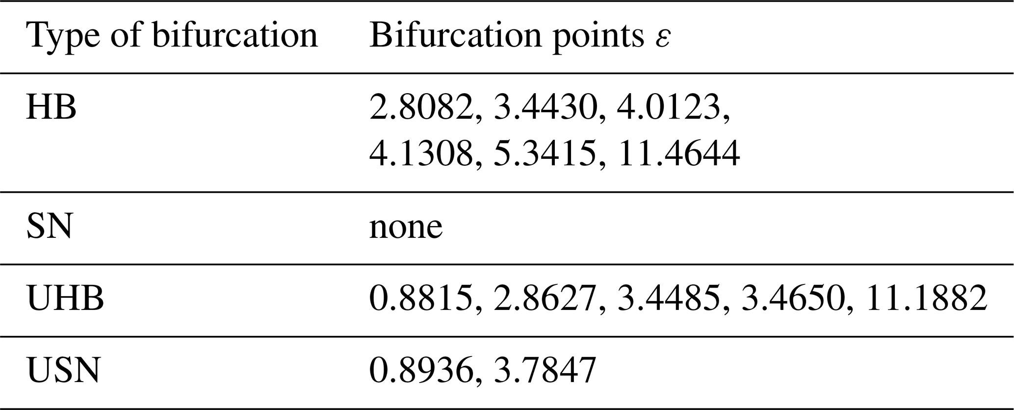
Figure 5 presents a detailed view of some of the features and bifurcation points in Fig. 4, indicating the eigenvalue structures of each curve and some specific bifurcation points. From Fig. 5, it can be seen that the system exhibits not only Hopf bifurcations at the transition between stable and unstable solutions, but also unstable Hopf bifurcations (UHBs) and unstable saddle-node bifurcations (USNs) on the unstable curves. The eigenvalue structures of each segment of the analytical solutions are indicated by arrows, and the bifurcation points are marked with black dots. It can be seen that the eigenvalue structures of the stable solutions are all (0, 0, 0 | 7, 0, 0), while the unstable solutions exhibit a variety of eigenvalue structures. Table 1 provides detailed information on the eigenvalue structures and stability of each segment of the system's solutions, while Table 2 lists the bifurcation points for each type of bifurcation that occurs in the system.

5 Analysis of the precision control of the solution

In this section, the multi-term generalized harmonic balance method is used to obtain the approximate analytical solution for the system's period-1 motion, and the time histories of displacement and trajectories as well as the harmonic amplitude and phase diagrams of the system are obtained. The accuracy of the analytical solution is verified by comparing it with the numerical solution.

In Fig. 6, the system parameters are Ω=2, α= 0.1, β₁= 1, β₂= 0.7, γ₁= 0.3444, γ₂= 0.03004, Q= 0.1, and ε= 13.26. The initial conditions (ICs) are x≈ 17.9867, $\dot{x}\approx$ -3.5406, t=0. The trajectories and amplitude diagrams obtained using HB2, HB4, HB6, and HB8 are compared with the analytical and numerical solutions. The black dots in Fig. 6a, c, e, and g represent the trajectories diagrams obtained by the numerical solution, and the red circles represent the trajectories diagrams obtained using the multi-term generalized harmonic balance method. The black dots in Fig. 6b, d, f, and h represent the amplitude–frequency diagrams obtained by the numerical solution using the fast Fourier transform, and the red crosses represent the harmonic amplitudes obtained using the multi-term generalized harmonic balance method. It can be seen that with the increase in the number of harmonic terms, the overlap between the analytical and numerical solutions in the trajectories diagrams increases and that the number of harmonic amplitude peaks corresponding to each harmonic term also increases. That is to say, the more harmonic terms are used, the lower the truncation error ignored by the analytical solution, and the more accurate the analytical solution obtained. When using the eight-term generalized harmonic balance method (HB8), the constant term is $a_{\mathrm{0}}=A_{\mathrm{0}}\approx$ 5.3907, and the harmonic amplitudes are A₁≈ 18.0306, A₂≈ 3.3413, A₃≈ 1.0545, A₄≈ 0.6765, A₅≈ 0.2279, A₆≈ 0.0867, A₇≈ 0.0369, and A₈≈ 0.0143. The maximum ignored harmonic amplitude is A₉≈ 0.0048, and the relative error is $A_{\mathrm{9}}/A_{\mathrm{1}}\approx$ $\mathrm{2.6621}\times {\mathrm{10}}^{-\mathrm{4}}$. The time histories of the displacement and trajectory diagrams based on HB8 are shown in Fig. 6i and j, respectively. The time histories of displacement of the periodic motion oscillates once within one period, and the harmonic phase φ_k ϵ [0, 2π), φ₀=π, indicates that the center of the periodic motion is on the left side of the velocity axis. The eigenvalue structure of the periodic motion is (1, 1, 0 | 5, 1, 0), which shows unstable period-1 motion.

Due to the sensitivity of nonlinear systems to initial conditions, the stability of the solution may change with different initial values under the same parameters. In Fig. 7, with system parameters Ω=2, α=0.1, β₁=1, β₂=0.7, γ₁=0.3444, γ₂=0.03004, Q= 0.1, and ε=13.26, the initial conditions are set to x≈ -22.4261, $\dot{x}\approx$ -31.9578, and t= 0. As shown in the time histories of the displacement diagram (Fig. 7a), the system experiences two oscillations within one period T, and the next period T repeats the periodic motion. Similarly, in the trajectory diagram Fig. 7b, the trajectory of periodic motion shows two circles in the phase plane. The harmonic amplitude values of the system are shown in Fig. 7c, with the constant term being $a_{\mathrm{0}}=A_{\mathrm{0}}\approx$ 2.7632, and the harmonic amplitudes A₁≈ 10.9170, A₂≈ 26.8007, A₃≈ 4.0060, A₄ ≈ 0.4221, A₅≈ 0.9852, A₆≈ 0.5713, A₇≈ 0.6012, A₈≈ 0.1761, and the maximum ignored harmonic amplitude A₉≈ 0.0354, with a relative error in $A_{\mathrm{9}}/A_{\mathrm{2}}\approx$ 1.3209 $\times {\mathrm{10}}^{-\mathrm{3}}$. The harmonic phase diagram of periodic motion is shown in Fig. 7d, with the harmonic phase φ_kϵ [0, 2π), and φ₀=π indicates that the center of periodic motion is located to the left of the velocity axis. The eigenvalue structure of periodic motion is (0, 0, 0 | 7, 0, 0), which represents stable period-1 motion.

In Fig. 8, with system parameters Ω= 2, α= 0.1, β₁= 1, β₂= 0.7, γ₁= 0.3444, γ₂= 0.03004, Q= 0.1, and ε= 2, the initial conditions (ICs) are x≈ -1.3399, $\dot{x}\approx$ 0.2507, and t= 0. The time histories of displacement diagram in Fig. 8a show that the system undergoes one oscillation within one period T, and the motion is similar to a sine function. In Fig. 8b, the trajectory of the periodic motion shows like an ellipse. The harmonic amplitude values are shown in Fig. 8c, with the constant term $a_{\mathrm{0}}=A_{\mathrm{0}}\approx \mathrm{0.8515}$, and the harmonic amplitudes A₁≈ 2.1762, A₂≈ 0.0154, A₃≈ $\mathrm{4.4121}\times {\mathrm{10}}^{-\mathrm{4}}$, $A_{\mathrm{4}}\approx \mathrm{4.3897}\times {\mathrm{10}}^{-\mathrm{4}}$, $A_{\mathrm{5}}\approx \mathrm{6.4662}\times {\mathrm{10}}^{-\mathrm{6}}$, $A_{\mathrm{6}}\approx \mathrm{2.9707}\times {\mathrm{10}}^{-\mathrm{7}}$, $A_{\mathrm{7}}\approx \mathrm{8.9344}\times {\mathrm{10}}^{-\mathrm{8}}$, and $A_{\mathrm{8}}\approx \mathrm{2.0399}\times {\mathrm{10}}^{-\mathrm{9}}$. The maximum harmonic amplitude that is neglected, A₉, is smaller than A8, and the relative error is no higher than $A_{\mathrm{8}}/A_{\mathrm{2}}\approx \mathrm{9.3737}\times {\mathrm{10}}^{-\mathrm{10}}$. The harmonic phase diagram of periodic motion is shown in Fig. 8d, with the harmonic phase φ_kϵ [0, 2π) and φ₀=π indicating that the center of periodic motion is to the left of the velocity axis. The eigenvalue structure of periodic motion is (0, 0, 0 | 7, 0, 0), indicating a stable period-1 motion.

In Fig. 9, the system parameters are Ω=2, α= 0.1, β₁= 1, β₂= 0.7, γ₁= 0.3444, γ₂= 0.03004, Q= 0.1, and ε= 4.56, and the initial conditions (ICs) are x≈ -4.3849, $\dot{x}\approx$ 0.8194, and t=0. From the time histories of the displacement diagram and the trajectory diagram, we see that the periodic motion exhibits a sinusoidal waveform and an elliptical shape, respectively. The amplitudes of harmonic components of the periodic motion are shown in Fig. 9c, with the constant term being $a_{\mathrm{0}}=A_{\mathrm{0}}\approx \mathrm{0.8515}$, and the harmonic amplitudes ranging from $A_{\mathrm{1}}\approx ,\mathrm{2.1762}$ to $A_{\mathrm{8}}\approx \mathrm{2.0399}\times {\mathrm{10}}^{-\mathrm{9}}$. The neglected maximum harmonic amplitude A₉ is less than A₈, with a relative error in $A_{\mathrm{8}}/A_{\mathrm{2}}\approx \mathrm{9.3737}\times {\mathrm{10}}^{-\mathrm{10}}$, and higher accuracy can be obtained by increasing the number of generalized harmonic components. The harmonic phase diagram of periodic motion is shown in Fig. 9d, with the harmonic phase φ_kϵ [0, 2π) and φ₀= 0 indicating that the center of the periodic motion is on the right side of the velocity axis. The eigenvalue structure of the periodic motion is (0, 0, 0 | 7, 0, 0), representing a stable period-1 motion.

6 Conclusions

This article establishes the dynamic equation of a gear system with clearance based on practical engineering applications and uses polynomials to mesh the segmented clearance function, and the analytic solution of the nonlinear dynamic system is obtained using the generalized harmonic balance method. A harmonic amplitude–amplitude of DTE characteristic diagram is obtained based on the generalized harmonic balance method. Through the analysis of the eigenvalue structure, the stability and bifurcation of the periodic motion are discussed in detail, and the influence of the external excitation amplitude on system stability and bifurcation is discussed. The following conclusions are obtained:

1. The system exhibits not only Hopf bifurcations at the transition between stable and unstable solutions, but also unstable Hopf bifurcations (UHB) and unstable saddle-node bifurcations (USN) on the unstable curves.

2. The more harmonic terms are used, the lower the truncation error ignored by the analytical solution, and the more accurate the analytical solution obtained. When using the eight-term generalized harmonic balance method (HB8), the precision requirement for the gear system can be satisfied in engineering application.

3. Due to the sensitivity of nonlinear systems to initial conditions, the stability of the solution may change with different initial values under the same parameters. In different initial conditions, the harmonic amplitude of the harmonic amplitude of the system changes the precision of the solution.

The stability of the strong nonlinear single-stage gear system with periodic motion is studied to provide a reference for selecting the corresponding parameters and initial conditions for the target periodic solution.