Joint kinematics and dynamics analysis of a 6-DOF loading and unloading industrial robot based on ADAMS and ANSYS

Accurate kinematics analysis and dynamics simulation are very important for checking the strength and stiffness of a robot's structure, which is helpful in the design of robot structures and judging the service life of a robot. In this study, a 6-DOF industrial robot was studied, and the ADAMS and ANSYS joint dynamics simulation method based on kinematics analysis was proposed. By establishing the floating coordinate system of the moving joint and using the transformation matrix to obtain the space pose of the robot end effector, the forward kinematics theoretical model was built. On the premise of the end pose, the rotation angle of the robot's moving joint was obtained by inverse transformation, and the inverse kinematics theoretical model was established. Then, according to the results of the kinematics analysis, ADAMS was used to simulate the whole process of loading and unloading of industrial robots to obtain the motion characteristics of each joint, and this was imported into ANSYS Workbench for transient dynamics analysis to obtain the bearing status of each part of the industrial robot in the loading and unloading process and to check the strength and stiffness of the structure of the loading and unloading robot. During the loading and unloading process, the maximum stress of the robot was 10.241 MPa and the maximum strain was 0.00014501, which were far less than the respective yield strengths of 304 stainless steel and 6061 aluminum alloy. The maximum deformation of the robot was 0.025272 mm, the overall deformation value was low, and the stiffness also met the design requirements. It can be seen clearly that the simulation results based on kinematics analysis are more real and reliable. Finally, this work proposes a novel, real, and accurate simulation method using ADAMS and ANSYS to carry out transient dynamics analysis to realize the strength and stiffness of the robot, which can be used to determine the support and service life of the industrial robot structure design.

1 Introduction

Today's industrial production line has been consistently transformed and upgraded in the direction of automation and intelligence (Wang et al., 2022a), and the overall efficiency and benefit of the manufacturing industry have witnessed a qualitative enhancement. The extensive application of diverse series of robots plays a crucial role in enhancing global industrial development and the operation of modern production systems. Industrial robots have advantages such as low manufacturing and operation costs, high flexibility, and strong operability and are a key component in the upgrade and transformation of production lines (Xiong et al., 2019). Currently, industrial robots are present on the industrial production line in fields such as automobiles, ships, and new energy. They can replace humans to undertake tasks like welding, handling, and spraying. Since they perform repetitive actions, over time, if the strength and stiffness of industrial robots are insufficient, the repeatability error of the end actuator will increase significantly. This will greatly reduce the accuracy and stability of the robot and subsequently reduce the production efficiency of the industrial production line, leading to a decline in the yield of the production line (Pham et al., 2022). Therefore, it is of utmost importance for industrial robots to have adequate rigid strength during movement to guarantee movement stability and reliability.

Kinematics analysis constitutes an advanced undertaking in the exploration of robot technology. Numerous researchers have conducted kinematics analysis based on Denavit–Hartenberg (D–H) criteria, which can determine the robot pose through the transformation of the connecting rod and the inversion of each joint angle through this pose. Wang et al. (2021) employed a new coordinate system transformation method to analyze the kinematics theory of 6-DOF robots with an open structural formula and were capable of extending the method to diverse types of industrial robots. An increasing number of novel methods are being utilized to study robot kinematics (Staicu et al., 2007). Forward and inverse kinematics analysis can employ Gaussian processes to drive soft robots (Relaño et al., 2023). The dual-rotation Lie group (Yang et al., 2018) can also be introduced, and the dual-torsion method can be used to deduce the kinematics of a 4-DOF robotic arm (Cibicik and Egeland, 2021). Thomas and Porta (2024) successfully addressed the inverse kinematics theory by obtaining a closure polynomial applying the distance geometry method. ADAMS and MATLAB simulations are commonly adopted by researchers for kinematics analysis of industrial robots (Wang et al., 2020). Wang et al. (2024) used a Lagrangian principle to conduct nonlinear dynamics analysis of industrial robots and verified its accuracy through the ADAMS simulation. Racz et al. (2022) utilized MATLAB to simulate the incremental formation of the robot and employed the inverse kinematics function and dynamics model to obtain the torque at the joint.

The accuracy and repeatability of the actuator constitute significant indicators for assessing the performance of industrial robots (Tiboni et al., 2024). Numerous scholars conduct research on robot kinematics to determine its positioning via the pose matrix, aiming to minimize its positioning error (D'Ago et al., 2024; Guan et al., 2024; Wang et al., 2018). To diminish the error of the robot arm during movement, Wu et al. (2024) employed statistical moment similarity to calculate the accuracy and optimal pose of the 6-DOF industrial robot. Guo et al. (2015) eliminated the maximum error of the actuator by more than 89 % through the analysis of absolute kinematics theory and took this as the standard. Korayem et al. (2006) carried out kinematics modeling through the transformation matrix and utilized visual processing methods to reduce the repeatability and position errors of assembly robots. Based on kinematics analysis, an increasing number of researchers combined the kinematics and dynamics of robots to study their vibration characteristics and optimize their dynamics features (Liu et al., 2021; Sattar et al., 2024; Wu et al., 2022). Through the evaluation and calibration of the robot's dynamics indicators, the robot has been applied successfully in diverse fields (Russo et al., 2024). Pham et al. (2022) performed inverse kinematics analysis of the Fanuc hexapod robot to predict the vibration characteristics of the platform. These researchers analyzed the robot's motion characteristics through kinematics, derived the vibration characteristics through dynamics, and obtained the end-effector pose and the optimal spatial position, thereby reducing errors and enhancing motion accuracy. Nevertheless, they failed to integrate the strength analysis of the robot structure and lacked the support of strength analysis during the robot's motion.

The strength analysis in the motion process is the key supporting role for the existing motion design scheme of industrial robots. The finite-element simulation results can provide guidance for the mechanical arm's stress conditions under different loads so as to optimize the design (Purandhara Sai Santosh et al., 2022). The stress and strain data are obtained through finite-element simulation, and the corresponding optimization can reduce the deformation of the overall structure (Roy et al., 2018), maximize the stiffness-to-weight ratio (Seth et al., 2022), improve the operating stability (Kornmaneesang et al., 2023), obtain the optimal solution of lightweight structure, save structural materials, and reduce manufacturing and use costs (Kouritem et al., 2022; Rubio et al., 2015). Canh et al. (2024) carried out lightweight optimization design for the two-arm service robot and checked the rigid strength of the robot structure, which successfully reduced the overall weight by 25 %. Ali et al. (2023), aiming at a 5-DOF industrial robot that undertakes sorting work on a production line, verified through statics analysis that the robot arm could maintain sufficient structural stiffness under large loads. Mepani et al. (2022) proposed a robot that can cook food independently to complete the production of dishes and performed a finite-element analysis of it. The stress and deformation meet the requirements and can maintain their structural integrity, which lays the technical groundwork for domestic cooking robots. However, these researchers only studied the rigid strength of the robot, did not analyze the robot kinematics, and lacked the data support of the robot dynamics characteristics.

Through the derivation and analysis of the kinematics theory of industrial robots and the dynamics simulation of the confirmed motion trajectory (Abu-Dakka et al., 2017), it can be verified that the proposed motion design scheme has no flaws (Raza et al., 2018). Wang et al. (2022b) developed a T-phage-simulated micro-robot with remarkable flexibility and great strength. The motion analysis of the robot was conducted using the finite-element method, and its carrying capacity was 6 times its own weight. Zhang et al. (2018) optimized the design of the 3-DOF manipulator, carried out forward and inverse kinematics analysis, and verified the stiffness strength to meet its application requirements. Friedrich et al. (2019) investigated the 6-DOF robot, which was capable of measuring the real force in the cutting process through static calculation, kinematics analysis, and rigid-body dynamics analysis. Only by integrating the rigid strength structure after the dynamics simulation of the robot can the robot kinematics analysis be significant; thereby, the overall structural design scheme of the industrial robot can be demonstrated to be reasonable (Sun et al., 2021; Yang et al., 2024).

In this study, an industrial robot for loading and unloading in the production line was designed. Based on the D-H construction principle, the floating coordinate system of each joint was established according to the initial posture of the loading and unloading industrial robot, and the kinematics equation was established by applying the continuous homogeneous transformation matrix to obtain the spatial position of each robot component in the process of motion, and the inverse kinematics solution was derived through this pose to obtain the joint angle, laying the groundwork for designing the optimal motion trajectory of this industrial robot. The industrial robot model was imported into ADAMS, the STEP function was utilized to plan the motion scheme, the joint drive function was defined, the entire process of loading and unloading of the industrial robot was simulated, the motion data of each joint were obtained, and then the joint motion data were used in ANSYS for transient dynamics analysis to examine the strength and stiffness of the industrial robot during motion. Finally, the rationality of the structure design and motion scheme of this industrial robot was verified, and it also provided reference and technical guidance for the structure optimization.

2 Kinematics analysis of industrial robots

2.1 Connecting-rod coordinate system

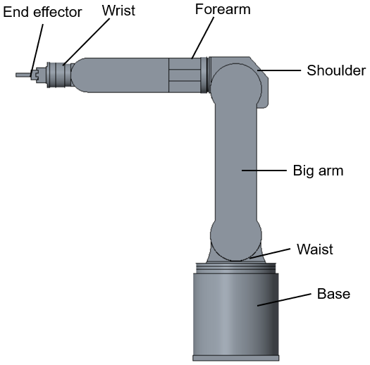
In this study, a 6-DOF robot for loading and unloading in the production line is designed, which includes a base, a big arm, a small arm, a wrist, an end effector, and other components. Figure 1 shows the initial position of the loading and unloading industrial robot. Six rotating joint floating coordinate systems were established according to Denavit–Hartenberg construction criteria and the initial positions in Fig. 2.

Figure 1 Initial position of the industrial robot.

Figure 2 Coordinate tie bar.

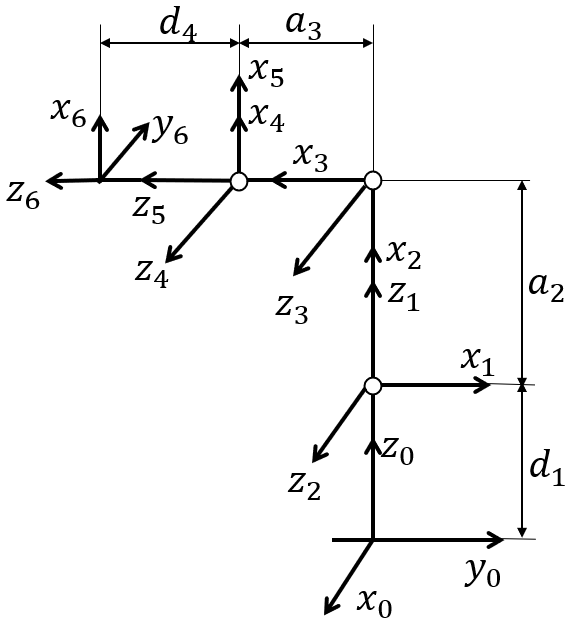
The meaning of the corresponding coordinate system parameters is as follows (Xu et al., 2023):

• 1.

  a_i is the length from z_i to z_i+1 in the x_i direction.

• 2.

  α_i is the angle from z_i to z_i+1 centered on x_i.

• 3.

  d_i is the length from x_i−1 to x_i in the z_i direction.

• 4.

  θ_i is the angle from x_i−1 to x_i centered on z_i.

All of the joints of the industrial robot are rotary joints, so θ_i is the joint variable and a_i, α_i, and d_i are constants. Table 1 shows the specific values of these four parameters of this industrial robot.

Table 1 Six-joint linkage parameter values.

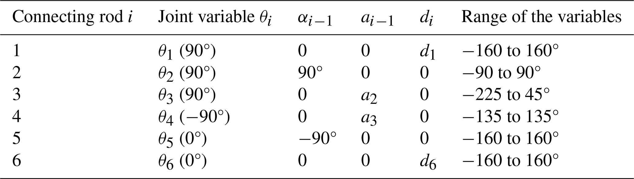
Parameter values: d₁ = 250 mm, a₂ = 385 mm, a₃ = 392 mm, and d₆ = 188 mm.

2.2 Forward kinematics equation of the industrial robot

The adjacent transformation matrix between the six joints is (Liu and Xu, 2018)

$$\begin{array}{}\text{(1)}& {}_i^{i-\mathrm{1}}T=\left[\begin{array}{cccc}c{\mathit{\theta }}_i& -s{\mathit{\theta }}_i& \mathrm{0}& a_{i-\mathrm{1}}\\ s{\mathit{\theta }}_{i}c{\mathit{\alpha }}_{i-\mathrm{1}}& c{\mathit{\theta }}_{i}c{\mathit{\alpha }}_{i-\mathrm{1}}& -s{\mathit{\alpha }}_{i-\mathrm{1}}& -d_{i}s{\mathit{\alpha }}_{i-\mathrm{1}}\\ s{\mathit{\theta }}_{i}s{\mathit{\alpha }}_{i-\mathrm{1}}& c{\mathit{\theta }}_{i}s{\mathit{\alpha }}_{i-\mathrm{1}}& c{\mathit{\alpha }}_{i-\mathrm{1}}& d_{i}c{\mathit{\alpha }}_{i-\mathrm{1}}\\ \mathrm{0}& \mathrm{0}& \mathrm{0}& \mathrm{1}\end{array}\right].\end{array}$$

By putting the values in Table 1 into Eq. (1), six joint transformation matrices can be obtained:

$$\begin{array}{rl}& {}_{\mathrm{1}}^{\mathrm{0}}T=\left[\begin{array}{cccc}{C}_{\mathrm{1}}& -S_{\mathrm{1}}& \mathrm{0}& \mathrm{0}\\ S_{\mathrm{1}}& C_{\mathrm{1}}& \mathrm{0}& \mathrm{0}\\ \mathrm{0}& \mathrm{0}& \mathrm{1}& d_{\mathrm{1}}\\ \mathrm{0}& \mathrm{0}& \mathrm{0}& \mathrm{1}\end{array}\right],{}_{\mathrm{2}}^{\mathrm{1}}T=\left[\begin{array}{cccc}{C}_{\mathrm{2}}& -S_{\mathrm{2}}& \mathrm{0}& \mathrm{0}\\ \mathrm{0}& \mathrm{0}& -\mathrm{1}& \mathrm{0}\\ S_{\mathrm{2}}& C_{\mathrm{2}}& \mathrm{0}& \mathrm{0}\\ \mathrm{0}& \mathrm{0}& \mathrm{0}& \mathrm{1}\end{array}\right],\\ & {}_{\mathrm{3}}^{\mathrm{2}}T=\left[\begin{array}{cccc}{C}_{\mathrm{3}}& -S_{\mathrm{3}}& \mathrm{0}& a_{\mathrm{3}}\\ S_{\mathrm{3}}& C_{\mathrm{3}}& \mathrm{0}& \mathrm{0}\\ \mathrm{0}& \mathrm{0}& \mathrm{1}& \mathrm{0}\\ \mathrm{0}& \mathrm{0}& \mathrm{0}& \mathrm{1}\end{array}\right],{}_{\mathrm{4}}^{\mathrm{3}}T=\left[\begin{array}{cccc}{C}_{\mathrm{4}}& -S_{\mathrm{4}}& \mathrm{0}& a_{\mathrm{4}}\\ S_{\mathrm{4}}& C_{\mathrm{4}}& \mathrm{0}& \mathrm{0}\\ \mathrm{0}& \mathrm{0}& \mathrm{1}& \mathrm{0}\\ \mathrm{0}& \mathrm{0}& \mathrm{0}& \mathrm{1}\end{array}\right],\\ & {}_{\mathrm{5}}^{\mathrm{4}}T=\left[\begin{array}{cccc}{C}_{\mathrm{5}}& -S_{\mathrm{5}}& \mathrm{0}& \mathrm{0}\\ \mathrm{0}& \mathrm{0}& \mathrm{1}& \mathrm{0}\\ -S_{\mathrm{5}}& -C_{\mathrm{5}}& \mathrm{0}& \mathrm{0}\\ \mathrm{0}& \mathrm{0}& \mathrm{0}& \mathrm{1}\end{array}\right],{}_{\mathrm{6}}^{\mathrm{5}}T=\left[\begin{array}{cccc}{C}_{\mathrm{6}}& -S_{\mathrm{6}}& \mathrm{0}& \mathrm{0}\\ S_{\mathrm{6}}& C_{\mathrm{6}}& \mathrm{0}& \mathrm{0}\\ \mathrm{0}& \mathrm{0}& \mathrm{1}& d_{\mathrm{6}}\\ \mathrm{0}& \mathrm{0}& \mathrm{0}& \mathrm{1}\end{array}\right].\end{array}$$

Multiply the six connecting-rod transformation matrices to obtain the robot actuator space pose (Feng et al., 2024):

$$\begin{array}{}\text{(2)}& \begin{array}{rl}{}_{\mathrm{6}}^{\mathrm{0}}T& ={}_{\mathrm{1}}^{\mathrm{0}}T\left({\mathit{\theta }}_{\mathrm{1}}\right){}_{\mathrm{2}}^{\mathrm{1}}T\left({\mathit{\theta }}_{\mathrm{2}}\right){}_{\mathrm{3}}^{\mathrm{2}}T\left({\mathit{\theta }}_{\mathrm{3}}\right){}_{\mathrm{4}}^{\mathrm{3}}T\left({\mathit{\theta }}_{\mathrm{4}}\right){}_{\mathrm{5}}^{\mathrm{4}}T\left({\mathit{\theta }}_{\mathrm{5}}\right){}_{\mathrm{6}}^{\mathrm{5}}T\left({\mathit{\theta }}_{\mathrm{6}}\right)\\ & =\left[\begin{array}{cccc}{n}_x& o_x& a_x& p_x\\ n_y& o_y& a_y& p_y\\ n_z& o_z& a_z& p_z\\ \mathrm{0}& \mathrm{0}& \mathrm{0}& \mathrm{1}\end{array}\right].\end{array}\end{array}$$

Equation (2) is a forward kinematics equation. The independent variable is the joint variable θ_i, and the dependent variable is the spatial position. The calculation results are as follows:

$$\begin{array}{}\text{(3)}& \left.\begin{array}{l}{n}_x=C_{\mathrm{1}}{C}_{\mathrm{2}}{C}_{\mathrm{34}}{C}_{\mathrm{56}}-C_{\mathrm{1}}{S}_{\mathrm{2}}{S}_{\mathrm{34}}{C}_{\mathrm{56}}-S_{\mathrm{1}}{S}_{\mathrm{56}},\\ n_y=S_{\mathrm{1}}{C}_{\mathrm{2}}{C}_{\mathrm{34}}{C}_{\mathrm{56}}-S_{\mathrm{1}}{S}_{\mathrm{2}}{S}_{\mathrm{34}}{C}_{\mathrm{56}}+C_{\mathrm{1}}{S}_{\mathrm{56}},\\ n_z=S_{\mathrm{2}}{C}_{\mathrm{34}}{C}_{\mathrm{56}}+C_{\mathrm{2}}{S}_{\mathrm{34}}{C}_{\mathrm{56}},\\ o_x=-C_{\mathrm{1}}{C}_{\mathrm{2}}{C}_{\mathrm{34}}{S}_{\mathrm{56}}+C_{\mathrm{1}}{S}_{\mathrm{2}}{S}_{\mathrm{34}}{S}_{\mathrm{56}}-S_{\mathrm{1}}{C}_{\mathrm{56}},\\ o_y=-S_{\mathrm{1}}{C}_{\mathrm{2}}{C}_{\mathrm{34}}{S}_{\mathrm{56}}+S_{\mathrm{1}}{S}_{\mathrm{2}}{S}_{\mathrm{34}}{S}_{\mathrm{56}}+C_{\mathrm{1}}{C}_{\mathrm{56}},\\ o_z=-S_{\mathrm{2}}{C}_{\mathrm{34}}{S}_{\mathrm{56}}-C_{\mathrm{2}}{S}_{\mathrm{34}}{S}_{\mathrm{56}},\\ a_x=-C_{\mathrm{1}}{C}_{\mathrm{2}}{S}_{\mathrm{34}}-C_{\mathrm{1}}{S}_{\mathrm{2}}{C}_{\mathrm{34}},\\ a_y=-S_{\mathrm{1}}{C}_{\mathrm{2}}{S}_{\mathrm{34}}-S_{\mathrm{1}}{S}_{\mathrm{2}}{C}_{\mathrm{34}},\\ a_z=-S_{\mathrm{2}}{S}_{\mathrm{34}}+C_{\mathrm{2}}{C}_{\mathrm{34}},\\ p_x=C_{\mathrm{1}}{C}_{\mathrm{2}}\left(-S_{\mathrm{34}}{d}_{\mathrm{6}}+C_{\mathrm{3}}{a}_{\mathrm{3}}+a_{\mathrm{2}}\right)-C_{\mathrm{1}}{S}_{\mathrm{2}}\left(C_{\mathrm{34}}{d}_{\mathrm{6}}+S_{\mathrm{3}}{a}_{\mathrm{3}}\right),\\ p_y=S_{\mathrm{1}}{C}_{\mathrm{2}}\left(-S_{\mathrm{34}}{d}_{\mathrm{6}}+C_{\mathrm{3}}{a}_{\mathrm{3}}+a_{\mathrm{2}}\right)-S_{\mathrm{1}}{S}_{\mathrm{2}}\left(C_{\mathrm{34}}{d}_{\mathrm{6}}+S_{\mathrm{3}}{a}_{\mathrm{3}}\right),\\ p_z=S_{\mathrm{2}}\left(-S_{\mathrm{34}}{d}_{\mathrm{6}}+C_{\mathrm{3}}{a}_{\mathrm{3}}+a_{\mathrm{2}}\right)+C_{\mathrm{2}}\left(C_{\mathrm{34}}{d}_{\mathrm{6}}+S_{\mathrm{3}}{a}_{\mathrm{3}}\right)+d_{\mathrm{1}},\end{array}\right\}.\end{array}$$

Among them are sin θ_i=S_i, cos θ_i=C_i, $C_{\mathrm{34}}=\cos \left({\mathit{\theta }}_{\mathrm{3}}+{\mathit{\theta }}_{\mathrm{4}}\right)=C_{\mathrm{3}}{C}_{\mathrm{4}}-S_{\mathrm{3}}{S}_{\mathrm{4}}$, $S_{\mathrm{34}}=\sin \left({\mathit{\theta }}_{\mathrm{3}}+{\mathit{\theta }}_{\mathrm{4}}\right)=S_{\mathrm{3}}{C}_{\mathrm{4}}+C_{\mathrm{3}}{S}_{\mathrm{4}}$, $C_{\mathrm{56}}=\cos \left({\mathit{\theta }}_{\mathrm{5}}+{\mathit{\theta }}_{\mathrm{6}}\right)=C_{\mathrm{5}}{C}_{\mathrm{6}}-S_{\mathrm{5}}{S}_{\mathrm{6}}$, and $S_{\mathrm{56}}=\sin \left({\mathit{\theta }}_{\mathrm{5}}+{\mathit{\theta }}_{\mathrm{6}}\right)=S_{\mathrm{5}}{C}_{\mathrm{6}}+C_{\mathrm{5}}{S}_{\mathrm{6}}$.

To check the correctness of the final pose matrix obtained, the initial values of each joint variable are brought in, and the value of the arm transformation matrix ${}_{\mathrm{6}}^{\mathrm{0}}T$ when ${\mathit{\theta }}_{\mathrm{1}}={\mathrm{90}}^{\circ },{\mathit{\theta }}_{\mathrm{2}}={\mathrm{90}}^{\circ },{\mathit{\theta }}_{\mathrm{3}}={\mathrm{90}}^{\circ },{\mathit{\theta }}_{\mathrm{4}}=-{\mathrm{90}}^{\circ },{\mathit{\theta }}_{\mathrm{5}}={\mathrm{0}}^{\circ },{\mathit{\theta }}_{\mathrm{6}}={\mathrm{0}}^{\circ }$ is calculated. The calculated results are as follows:

$${}_{\mathrm{6}}^{\mathrm{0}}T=\left[\begin{array}{cccc}\mathrm{0}& -\mathrm{1}& \mathrm{0}& \mathrm{0}\\ \mathrm{0}& \mathrm{0}& -\mathrm{1}& -(d_{\mathrm{6}}+a_{\mathrm{3}})\\ \mathrm{1}& \mathrm{0}& \mathrm{0}& a_{\mathrm{2}}+d_{\mathrm{1}}\\ \mathrm{0}& \mathrm{0}& \mathrm{0}& \mathrm{1}\end{array}\right].$$

This is exactly the same as shown in Fig. 2.

The transformation matrix ${}_{\mathrm{6}}^{\mathrm{0}}T$ represents the pose of the industrial robot claw in the first coordinate system. When each θ_i is determined, the pose matrix of the robot actuator can be acquired.

2.3 Inverse kinematics of industrial robots

The inverse kinematics is as follows: given the value of ${}_{\mathrm{6}}^{\mathrm{0}}T$, find all possible solutions for each θ_i. The kinematics equation of the 6-DOF robot is rewritten as

$$\begin{array}{}\text{(4)}& \begin{array}{rl}{}_{\mathrm{6}}^{\mathrm{0}}T& =\left[\begin{array}{cccc}{n}_x& o_x& a_x& p_x\\ n_y& o_y& a_y& p_y\\ n_z& o_z& a_z& p_z\\ \mathrm{0}& \mathrm{0}& \mathrm{0}& \mathrm{1}\end{array}\right]\\ & ={}_{\mathrm{1}}^{\mathrm{0}}T\left({\mathit{\theta }}_{\mathrm{1}}\right){}_{\mathrm{2}}^{\mathrm{1}}T\left({\mathit{\theta }}_{\mathrm{2}}\right){}_{\mathrm{3}}^{\mathrm{2}}T\left({\mathit{\theta }}_{\mathrm{3}}\right){}_{\mathrm{4}}^{\mathrm{3}}T\left({\mathit{\theta }}_{\mathrm{4}}\right){}_{\mathrm{5}}^{\mathrm{4}}T\left({\mathit{\theta }}_{\mathrm{5}}\right){}_{\mathrm{6}}^{\mathrm{5}}T\left({\mathit{\theta }}_{\mathrm{6}}\right).\end{array}\end{array}$$

The corresponding inverse transformation matrix is simultaneously left multiplied by Eq. (4), and the values of each joint variable θ_i are solved (Tarng et al., 2024).

2.3.1 Solve for θ₁

Multiply Eq. (4) by ${}_{\mathrm{1}}^{\mathrm{0}}{T}^{-\mathrm{1}}\left({\mathit{\theta }}_{\mathrm{1}}\right)$ to the left, which gives

$$\begin{array}{}\text{(5)}& \left[\begin{array}{cccc}{C}_{\mathrm{1}}& S_{\mathrm{1}}& \mathrm{0}& \mathrm{0}\\ -S_{\mathrm{1}}& C_{\mathrm{1}}& \mathrm{0}& \mathrm{0}\\ \mathrm{0}& \mathrm{0}& \mathrm{1}& -d_{\mathrm{1}}\\ \mathrm{0}& \mathrm{0}& \mathrm{0}& \mathrm{1}\end{array}\right]=\left[\begin{array}{cccc}{n}_x& o_x& a_x& p_x\\ n_y& o_y& a_y& p_y\\ n_z& o_z& a_z& p_z\\ \mathrm{0}& \mathrm{0}& \mathrm{0}& \mathrm{1}\end{array}\right]={}_{\mathrm{6}}^{\mathrm{1}}T.\end{array}$$

If the elements (2,3) at both ends of Eq. (5) correspond equally, we can get

$$\begin{array}{}\text{(6)}& {\mathit{\theta }}_{\mathrm{1}}=a\tan \mathrm{2}\left(p_y,p_x\right).\end{array}$$

2.3.2 Solve for θ₂

Let the elements (1,3), (3,3), (1,4), and (3,4) on both sides of the matrix Eq. (5) correspond to each other, and the equations obtained are as follows:

$$\begin{array}{}\text{(7)}& \left\{\begin{array}{l}{C}_{\mathrm{1}}{a}_x+S_{\mathrm{1}}{a}_y=-C_{\mathrm{2}}{S}_{\mathrm{34}}-S_{\mathrm{2}}{C}_{\mathrm{34}},\\ a_z=-S_{\mathrm{2}}{S}_{\mathrm{34}}+C_{\mathrm{2}}{C}_{\mathrm{34}},\\ C_{\mathrm{1}}{p}_x+S_{\mathrm{1}}{p}_y=C_{\mathrm{2}}\left(-S_{\mathrm{34}}{d}_{\mathrm{6}}+C_{\mathrm{3}}{a}_{\mathrm{3}}+a_{\mathrm{2}}\right)-S_{\mathrm{2}}\left(C_{\mathrm{34}}{d}_{\mathrm{6}}+S_{\mathrm{3}}{a}_{\mathrm{3}}\right),\\ p_z-d_{\mathrm{1}}=S_{\mathrm{2}}\left(-S_{\mathrm{34}}{d}_{\mathrm{6}}+C_{\mathrm{3}}{a}_{\mathrm{3}}+a_{\mathrm{2}}\right)+C_{\mathrm{2}}\left(C_{\mathrm{34}}{d}_{\mathrm{6}}+S_{\mathrm{3}}{a}_{\mathrm{3}}\right).\end{array}\right.\end{array}$$

This is simplified as follows:

$$\begin{array}{}\text{(8)}& \begin{array}{rl}& (C_{\mathrm{1}}{p}_x+S_{\mathrm{1}}{p}_y-C_{\mathrm{1}}{a}_x{d}_{\mathrm{6}}-S_{\mathrm{1}}{a}_y{d}_{\mathrm{6}})C_{\mathrm{2}}+\left(p_z-d_{\mathrm{1}}-a_z{d}_{\mathrm{6}}\right)S_{\mathrm{2}}\\ & ={\displaystyle \frac{(C_{\mathrm{1}}{p}_x+S_{\mathrm{1}}{p}_y-C_{\mathrm{1}}{a}_x{d}_{\mathrm{6}}-S_{\mathrm{1}}{a}_y{d}_{\mathrm{6}}{)}^{\mathrm{2}}+(p_z-d_{\mathrm{1}}-a_z{d}_{\mathrm{6}}{)}^{\mathrm{2}}+a_{\mathrm{2}}^{\mathrm{2}}-a_{\mathrm{3}}^{\mathrm{2}}}{\mathrm{2}{a}_{\mathrm{2}}}}.\end{array}\end{array}$$

Using trigonometric substitution,

$$\begin{array}{}\text{(9)}& \left\{\begin{array}{l}\mathit{\rho }\sin \mathrm{\Phi }=C_{\mathrm{1}}{p}_x+S_{\mathrm{1}}{p}_y-C_{\mathrm{1}}{a}_x{d}_{\mathrm{6}}-S_{\mathrm{1}}{a}_y{d}_{\mathrm{6}},\\ \mathit{\rho }\cos \mathrm{\Phi }=p_z-d_{\mathrm{1}}-a_z{d}_{\mathrm{6}},\end{array}\right.\end{array}$$

where ρ and Φ are defined as

$$\begin{array}{}\text{(10)}& {\displaystyle }\mathit{\rho }=\sqrt{(C_{\mathrm{1}}{p}_x+S_{\mathrm{1}}{p}_y-C_{\mathrm{1}}{a}_x{d}_{\mathrm{6}}-S_{\mathrm{1}}{a}_y{d}_{\mathrm{6}}{)}^{\mathrm{2}}+(p_z-d_{\mathrm{1}}-a_z{d}_{\mathrm{6}}{)}^{\mathrm{2}}},\text{(11)}& {\displaystyle }\mathrm{\Phi }=a\tan \mathrm{2}(C_{\mathrm{1}}{p}_x+S_{\mathrm{1}}{p}_y-C_{\mathrm{1}}{a}_x{d}_{\mathrm{6}}-S_{\mathrm{1}}{a}_y{d}_{\mathrm{6}},p_z-d_{\mathrm{1}}-a_z{d}_{\mathrm{6}}).\end{array}$$

By simplification, we can get

$$\begin{array}{}\text{(12)}& {\displaystyle }\mathit{\rho }\sin \mathrm{\Phi }{C}_{\mathrm{2}}+\mathit{\rho }\cos \mathrm{\Phi }{S}_{\mathrm{2}}=k\text{(13)}& {\displaystyle }\mathrm{\Phi }+{\mathit{\theta }}_{\mathrm{2}}=a\tan \mathrm{2}({\displaystyle \frac{k}{\mathit{\rho }}},\pm \sqrt{\mathrm{1}-({\displaystyle \frac{k}{\mathit{\rho }}}{)}^{\mathrm{2}}}),\end{array}$$

where k is defined as

$$\begin{array}{}\text{(14)}& \begin{array}{rl}& k=\\ & {\displaystyle \frac{(C_{\mathrm{1}}{p}_x+S_{\mathrm{1}}{p}_y-C_{\mathrm{1}}{a}_x{d}_{\mathrm{6}}-S_{\mathrm{1}}{a}_y{d}_{\mathrm{6}}{)}^{\mathrm{2}}+(p_z-d_{\mathrm{1}}-a_z{d}_{\mathrm{6}}{)}^{\mathrm{2}}+a_{\mathrm{2}}^{\mathrm{2}}-a_{\mathrm{3}}^{\mathrm{2}}}{\mathrm{2}{a}_{\mathrm{2}}}}.\end{array}\end{array}$$

So, we can find out θ₂:

$$\begin{array}{}\text{(15)}& \begin{array}{rl}{\mathit{\theta }}_{\mathrm{2}}& =a\tan \mathrm{2}(k,\pm \sqrt{{\mathit{\rho }}^{\mathrm{2}}-k^{\mathrm{2}}})-a\tan \mathrm{2}(C_{\mathrm{1}}{p}_x+S_{\mathrm{1}}{p}_y\\ & -C_{\mathrm{1}}{a}_x{d}_{\mathrm{6}}-S_{\mathrm{1}}{a}_y{d}_{\mathrm{6}},p_z-d_{\mathrm{1}}-a_z{d}_{\mathrm{6}}).\end{array}\end{array}$$

The positive and negative signs correspond to the two solutions of θ₂.

2.3.3  Solve for θ₃

$$\begin{array}{}\text{(16)}& \begin{array}{rl}{\mathit{\theta }}_{\mathrm{23}}& ={\mathit{\theta }}_{\mathrm{2}}+{\mathit{\theta }}_{\mathrm{3}}=a\tan \mathrm{2}(p_z-d_{\mathrm{1}}-a_z{d}_{\mathrm{6}}-S_{\mathrm{2}}{a}_{\mathrm{2}},C_{\mathrm{1}}{p}_x\\ & +S_{\mathrm{1}}{p}_y-C_{\mathrm{1}}{a}_x{d}_{\mathrm{6}}-S_{\mathrm{1}}{a}_y{d}_{\mathrm{6}}-C_{\mathrm{2}}{a}_{\mathrm{2}})\end{array}\end{array}$$

So, we can figure out

$$\begin{array}{}\text{(17)}& \begin{array}{rl}{\mathit{\theta }}_{\mathrm{3}}& =a\tan \mathrm{2}(p_z-d_{\mathrm{1}}-a_z{d}_{\mathrm{6}}-S_{\mathrm{2}}{a}_{\mathrm{2}},C_{\mathrm{1}}{p}_x+S_{\mathrm{1}}{p}_y\\ & -C_{\mathrm{1}}{a}_x{d}_{\mathrm{6}}-S_{\mathrm{1}}{a}_y{d}_{\mathrm{6}}-C_{\mathrm{2}}{a}_{\mathrm{2}})\\ & -a\tan \mathrm{2}\left(k,\pm \sqrt{{\mathit{\rho }}^{\mathrm{2}}-k^{\mathrm{2}}}\right)+a\tan \mathrm{2}(C_{\mathrm{1}}{p}_x+S_{\mathrm{1}}{p}_y\\ & -C_{\mathrm{1}}{a}_x{d}_{\mathrm{6}}-S_{\mathrm{1}}{a}_y{d}_{\mathrm{6}},p_z-d_{\mathrm{1}}-a_z{d}_{\mathrm{6}}).\end{array}\end{array}$$

Based on the four combinations of θ₁ and θ₂ solutions, four different θ₂₃ values can be obtained, and thus four possible solutions of θ₃ can be obtained.

2.3.4 Solve for θ₄

Multiply both ends of Eq. (4) by the inverse ${}_{\mathrm{3}}^{\mathrm{0}}{T}^{-\mathrm{1}}$. If the elements (1,3) and (2,3) at both ends of the previous equation correspond equally, we can get

$$\begin{array}{}\text{(18)}& \left\{\begin{array}{l}{C}_{\mathrm{1}}{C}_{\mathrm{23}}{a}_x+S_{\mathrm{1}}{C}_{\mathrm{23}}{a}_y+S_{\mathrm{23}}{a}_z=-S_{\mathrm{4}},\\ -C_{\mathrm{1}}{S}_{\mathrm{23}}{a}_x-S_{\mathrm{1}}{S}_{\mathrm{23}}{a}_y+C_{\mathrm{23}}{a}_z=C_{\mathrm{4}}.\end{array}\right.\end{array}$$

Since θ₁, θ₂, and θ₃ are already solved, we can solve for θ₄:

$$\begin{array}{}\text{(19)}& \begin{array}{rl}{\mathit{\theta }}_{\mathrm{4}}& =a\tan \mathrm{2}(C_{\mathrm{1}}{C}_{\mathrm{23}}{a}_x+S_{\mathrm{1}}{C}_{\mathrm{23}}{a}_y+S_{\mathrm{23}}{a}_z,C_{\mathrm{1}}{S}_{\mathrm{23}}{a}_x\\ & +S_{\mathrm{1}}{S}_{\mathrm{23}}{a}_y-C_{\mathrm{23}}{a}_z).\end{array}\end{array}$$

2.3.5 Solve for θ₅

Multiply both ends of Eq. (4) by the inverse ${}_{\mathrm{5}}^{\mathrm{0}}{T}^{-\mathrm{1}}$ and expand the previous matrix equation so that the elements (1,4) at both ends correspond to the same. Then,

$$\begin{array}{}\text{(20)}& \begin{array}{l}{C}_{\mathrm{5}}[C_{\mathrm{4}}\left(C_{\mathrm{1}}{C}_{\mathrm{23}}{p}_x+S_{\mathrm{1}}{C}_{\mathrm{23}}{p}_y+S_{\mathrm{23}}{p}_z-C_{\mathrm{3}}{a}_{\mathrm{2}}-S_{\mathrm{23}}{d}_{\mathrm{1}}\right)\\ +S_{\mathrm{4}}(-C_{\mathrm{1}}{S}_{\mathrm{23}}{p}_x-S_{\mathrm{1}}{S}_{\mathrm{23}}{p}_y+C_{\mathrm{23}}{p}_z+S_{\mathrm{3}}{a}_{\mathrm{2}}-C_{\mathrm{23}}{d}_{\mathrm{1}})\\ -C_{\mathrm{4}}{a}_{\mathrm{3}}]-S_{\mathrm{5}}\left(S_{\mathrm{1}}{p}_x-C_{\mathrm{1}}{p}_y\right)=\mathrm{0}.\end{array}\end{array}$$

So, we can get

$$\begin{array}{}\text{(21)}& \begin{array}{rl}{\mathit{\theta }}_{\mathrm{5}}=& a\tan \mathrm{2}\left(C_{\mathrm{4}}\right(C_{\mathrm{1}}{C}_{\mathrm{23}}{p}_x+S_{\mathrm{1}}{C}_{\mathrm{23}}{p}_y+S_{\mathrm{23}}{p}_z-C_{\mathrm{3}}{a}_{\mathrm{2}}\\ & -S_{\mathrm{23}}{d}_{\mathrm{1}})+S_{\mathrm{4}}(-C_{\mathrm{1}}{S}_{\mathrm{23}}{p}_x-S_{\mathrm{1}}{S}_{\mathrm{23}}{p}_y+C_{\mathrm{23}}{p}_z\\ & +S_{\mathrm{3}}{a}_{\mathrm{2}}-C_{\mathrm{23}}{d}_{\mathrm{1}})-C_{\mathrm{4}}{a}_{\mathrm{3}},S_{\mathrm{1}}{p}_x-C_{\mathrm{1}}{p}_y).\end{array}\end{array}$$

Figure 3 ADAMS simulation model.

2.3.6 Solve for θ₆

If the elements (1,1) and (2,1) at both ends correspond equally, then

$$\begin{array}{}\text{(22)}& \left\{\begin{array}{l}{C}_{\mathrm{5}}[C_{\mathrm{4}}\left(C_{\mathrm{1}}{C}_{\mathrm{23}}{n}_x+S_{\mathrm{1}}{C}_{\mathrm{23}}{n}_y+S_{\mathrm{23}}{n}_z\right)\\ +S_{\mathrm{4}}\left(-C_{\mathrm{1}}{S}_{\mathrm{23}}{n}_x-S_{\mathrm{1}}{S}_{\mathrm{23}}{n}_y+C_{\mathrm{23}}{n}_z\right)]\\ -S_{\mathrm{5}}\left(S_{\mathrm{1}}{n}_x-C_{\mathrm{1}}{n}_y\right)=C_{\mathrm{6}},\\ -S_{\mathrm{5}}[C_{\mathrm{4}}\left(C_{\mathrm{1}}{C}_{\mathrm{23}}{n}_x+S_{\mathrm{1}}{C}_{\mathrm{23}}{n}_y+S_{\mathrm{23}}{n}_z\right)\\ +S_{\mathrm{4}}\left(-C_{\mathrm{1}}{S}_{\mathrm{23}}{n}_x-S_{\mathrm{1}}{S}_{\mathrm{23}}{n}_y+C_{\mathrm{23}}{n}_z\right)]\\ -C_{\mathrm{5}}\left(S_{\mathrm{1}}{n}_x-C_{\mathrm{1}}{n}_y\right)=S_{\mathrm{6}}.\end{array}\right.\end{array}$$

This gives us a closed solution:

$$\begin{array}{}\text{(23)}& {\mathit{\theta }}_{\mathrm{6}}=a\tan \mathrm{2}\left(S_{\mathrm{6}},C_{\mathrm{6}}\right).\end{array}$$

The inverse kinematics have been obtained. When the pose of the effector is known, industrial robot 6's joint angle can be solved (Gao et al., 2018). Similarly, the pose coordinates of the actuator can be solved when the motion angles of the six joints are known (Cao et al., 2022). The establishment of forward and inverse kinematics equations is the technical basis for motion planning and ADAMS simulation of industrial robots, which is helpful for realizing the analysis of transient dynamics in ANSYS and paving the way for later trajectory planning and motion control. Only because of the limitations of the loading and unloading industrial robot itself, and considering the movement time, rhythm, and energy consumption, some solutions cannot be realized, so it is necessary to take the most conducive ones for the work of the industrial robot for the set of solutions so as to achieve the best motion planning of loading and unloading robots.

3 Kinematics simulation of the industrial robot

3.1 Set constraints and drivers

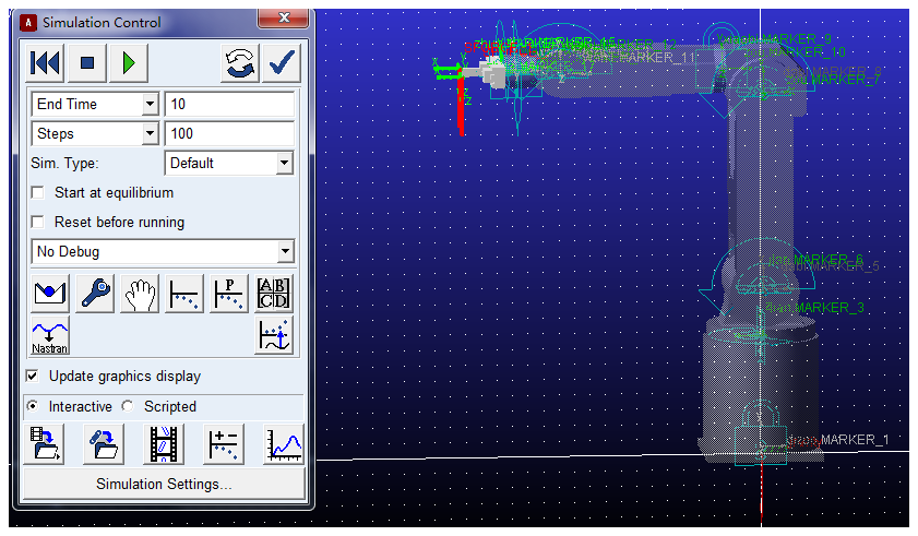
To obtain the actual force condition, the entire loading and unloading process of the mechanical arm will be simulated. The 3D model of the industrial robot is converted to X_T format and imported into ADAMS to conduct the kinematics simulation. As depicted in Fig. 3, a corresponding constraint relationship is established for the motion relationship of each joint, a drive was added to each rotating pair, and a concentrated force of 196 N is applied to the end effector to replace a 20 kg weight with a concentrated force. Each of the two claws of the end effector shared a force of 98 N. The simulation time is 10 s, and the number of steps is 100.

The STEP function is used to define each joint rotation pair, and the drive function is applied in turn to obtain six rotating joint motion laws (Guiju and Caiyuan, 2018).

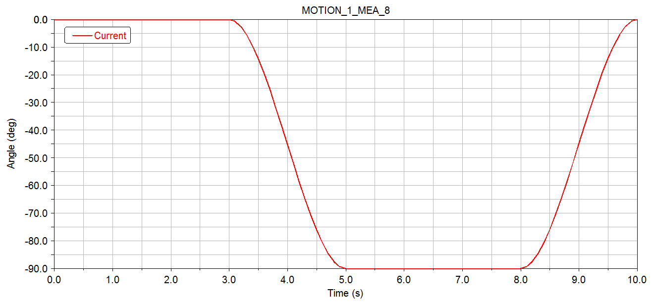
• First rotational joints: STEP(time,3,0,5,90d) + STEP(time,8,0,10,−90d).

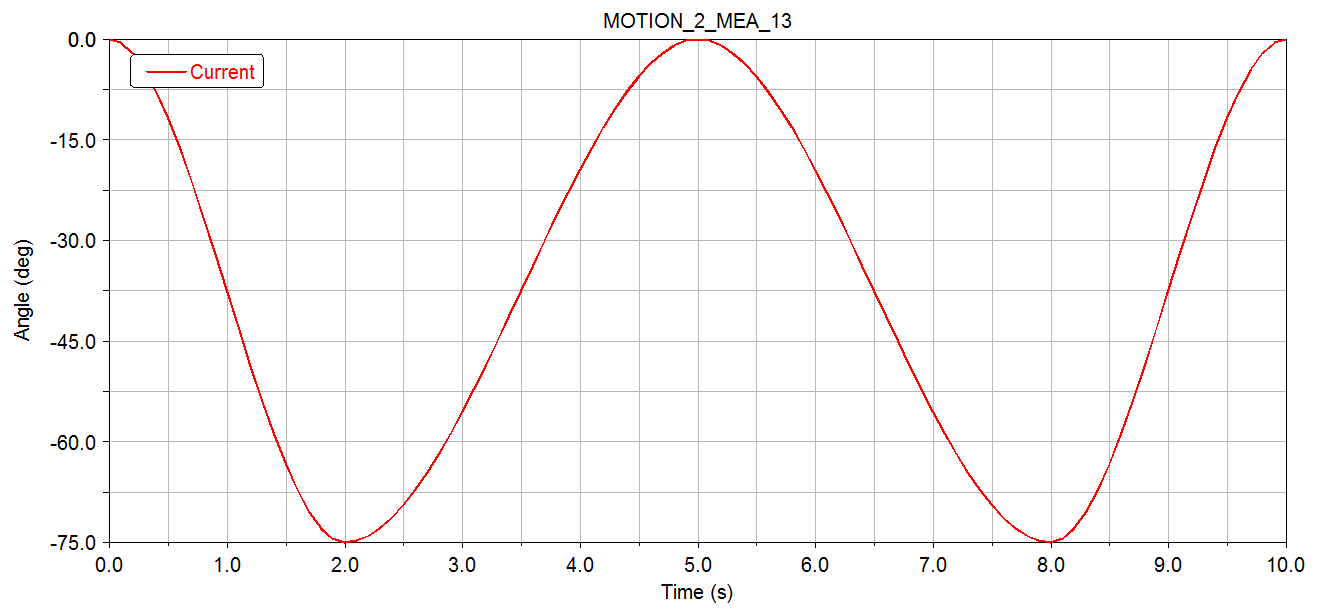
• Second rotational joints: STEP(time,0,0,2,75d) + STEP(time,2,0,5,−75d) + STEP(time,5,0,8,75d) + STEP(time,8,0,10,−75d).

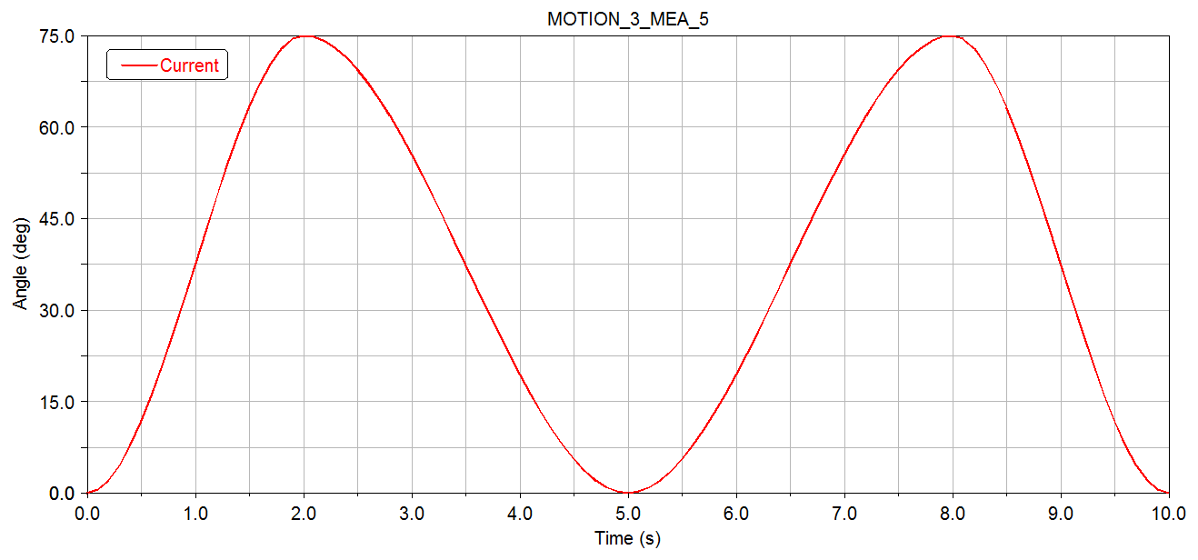
• Third rotational joints: STEP(time,0,0,2,−75d) + STEP(time,2,0,5,75d) + STEP(time,5,0,8,−75d) + STEP(time,8,0,10,75d).

• The fourth, fifth, and sixth rotator joints are all 0.

• The force at the end of the actuator is STEP(time,1.99,0,2,98) + STEP(time,7.99,0,8,−98).

Figure 4 First joint rotation rule.

Figure 5 Second joint rotation rule.

3.2 Analysis of the motion simulation results

After the simulation, the angular variation curves of each rotating joint with respect to time can be acquired. Figure 4 shows the motion law of the first joint, i.e., the rotation law of the waist joint. This waist joint starts to rotate to 90° in the third second after the robot picks up the material and starts to reset and rotate in the eighth second after the robot puts down the material. The motion rules of the second joint, i.e., the shoulder joint, are expressed in the form of images in Fig. 5. The shoulder joint takes 2 s to rotate down 75° to catch the material and then turns back. When the waist joint rotates to the designated position, the material is returned to its original position. Figure 6 shows the rotation and change curve of the elbow joint of the third joint, i.e., the elbow joint of the industrial robot. The elbow joint expands outward to grasp the material, and its movement law is the same as that of the shoulder joint, but the steering is different from that of the shoulder joint. Finally, the curve of the angle change is derived in the form of the data analysis table, which is convenient for the subsequent transient dynamics analysis of industrial robots.

Figure 6 Third joint rotation rule.

4 Transient dynamics analysis of industrial robots

4.1 Import data

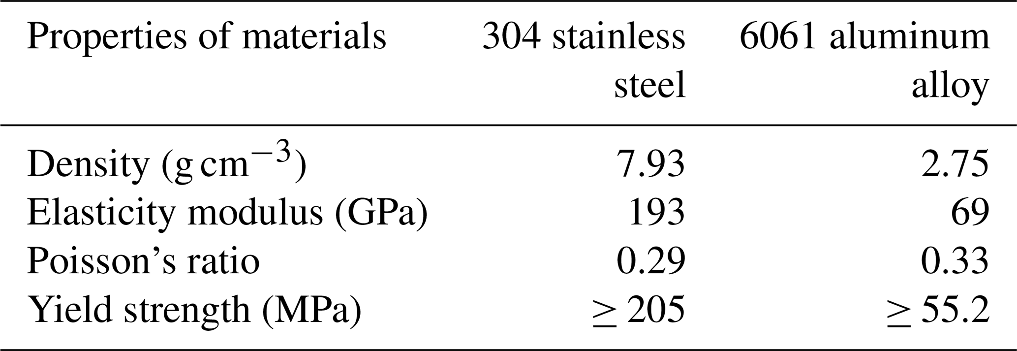
Add the corresponding rotation pairs and material properties. The base and waist of the industrial robot are made of 304 stainless steel, and the other components are made of 6061 aluminum alloy. The material properties of 304 and 6061 are shown in Table 2. The solution time is 10 s and the number of steps is 100, which is consistent with the numbers in ADAMS. Using automatic grid division, the number of grid units in the industrial robot model is 8802 and the number of nodes is 17 109.

Table 2 Properties of materials.

Figure 7 Import the second joint angle value.

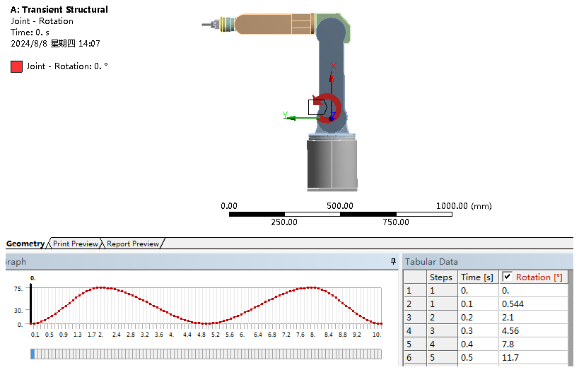
The joint angle change value simulated in ADAMS of the industrial robot is imported into the model joint in ANSYS Workbench. Take the second joint as an example, as shown in Fig. 7, and import other joints in turn. Because the driving torque applied in ADAMS is opposite to that applied to some joints in ANSYS Workbench, the graph will be exactly the opposite.

Figure 8 Stress distribution.

Figure 9 Strain distribution.

4.2 Analysis of the transient dynamics results

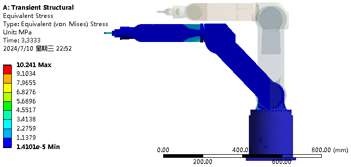
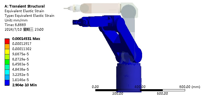
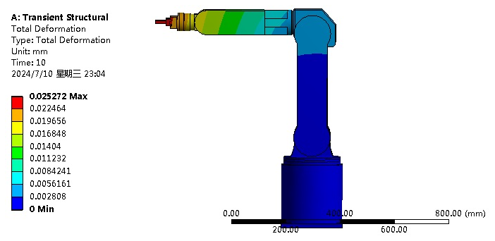
The results of the ADAMS simulation are imported into ANSYS Workbench to realize the transient dynamics analysis, simulate the stress condition of industrial robots in the real loading and unloading process, and check their strength and stiffness under the motion scheme. In Fig. 8, the stress distribution of the entire structure in the process of loading and unloading is more obvious in the shoulder, elbow, and end-actuator parts of the robot, and it is also the part where the robot structure should be optimized further in the latter work. However, the maximum stress in the movement process is 10.241 MPa, which is far less than the respective yield strengths of 304 stainless steel and 6061 aluminum alloy. The bearing strain of the overall structure of the robot is expressed in Fig. 9. Since the overall stress is low, the overall structural strain of the robot is also at a low level, and its maximum strain is 0.00014531. Figure 10 shows the deformation distribution and stiffness of the industrial robot in the process of this movement. The maximum deformation generated by the robot is 0.025272 mm. A low deformation value indicates that its stiffness is sufficiently reliable. From the results of the transient dynamics, the industrial robot has sufficient strength and high stiffness. The overall performance meets the work requirements and also verifies the reliability and rationality of the design. At the same time, it also provides technical guidance for the latter's structural optimization and makes clear the direction of the optimization.

Figure 10 Overall deformation of the structure.

5 Conclusions

In this work, the design, simulation, and finite-element analysis of industrial robots were completed. According to the requirements, the 3D modeling of the industrial robot was completed by Pro-E. The kinematics analysis of the initial position of the industrial robot was completed. Firstly, based on the D-H coordinate method, the floating coordinate system was set up for the kinematics joint of the model, and the parameters of each joint were obtained. Secondly, the kinematics theoretical model was successfully built. The pose matrix was calculated, and the forward kinematics analysis was completed. Then, the final solution was derived according to the forward kinematics theory, and the inverse kinematics analysis was completed.

Each part of the robot was converted into X_T format and imported into the ADAMS simulation software in turn. Relevant parameters were set, corresponding connection pairs and drivers were added to the joints, a STEP function model was established, and the STEP function was used for the driving. The simulation time and number of steps were set to simulate the actual motion process of the industrial robot during loading and unloading. Then, the variation curves of each rotating joint angle of the model were obtained and exported in the form of a data analysis table.

The angle changes of each rotating joint obtained by the ADAMS simulation were imported into the joint rotating pair of the industrial robot in ANSYS Workbench, and the transient dynamics analysis was realized in ANSYS Workbench. During the loading and unloading process, the actual maximum stress was 10.241 MPa and the maximum strain was 0.00014501, which was much lower than the yield strength of the robot structural materials. The maximum deformation of the robot was 0.025272 mm, and its overall deformation value was low; i.e., the stiffness was in a high state. The transient dynamics simulation obtained the actual loading status of the industrial robot, and the analysis fully considered the structure and inertial force of the industrial robot itself and obtained the overall stress, strain, and deformation distribution of the industrial robot. It was intuitively and vividly shown that the overall strength and stiffness met the design requirements. Furthermore, the overall structural rationality of the 6-DOF loading and unloading robot was verified, and the technical groundwork was also laid for the structural optimization in the later stage.