A control strategy for shipboard stabilization platforms based on a fuzzy adaptive proportional–integral–derivative (PID) control architecture

To address the precision degradation of marine equipment under coupled hydrodynamic disturbances, this study develops a 6-degree-of-freedom (6-DOF) stabilization platform with a fuzzy adaptive proportional–integral–derivative (PID) control architecture. The kinematic model is established via analysis based on the virtual-work principle, complemented by Monte Carlo simulations for workspace characterization. A fuzzy inference engine dynamically adjusts PID parameters through rule-based adaptation, demonstrating superior disturbance rejection. Comparative simulations indicate a 50 % reduction in settling time (7.0 s to 3.5 s), zero overshoot, and < 0.03° steady-state tracking error under 2 Hz sinusoidal excitation. A human–machine interface (HMI) for the shipboard stabilization platform is developed using the Qt Creator framework, integrating real-time trajectory tracking and parameter tuning. The research advances marine stabilization technology through mechanical optimization via virtual-work modeling and control enhancement via fuzzy–PID synthesis. Experimental validation confirms the framework's capability to maintain sub −0.03° precision under dynamic maritime conditions.

1 Introduction

Under combined marine wind and wave effects, ships exhibit complex multi-degree-of-freedom motions, including roll, pitch, and yaw (RPY), significantly compromising the operational accuracy of onboard equipment (Tu et al., 2022; Qiang et al., 2024). Current research on shipboard stabilization platforms focuses on structural design and control strategies (Chen et al., 2024; Liu et al., 2025; Mei et al., 2021).

In structural design, novel parallel mechanisms dominate recent advancements. Liu et al. (2023) developed a 6-degree-of-freedom (6-DOF) parallel platform with motion prediction compensation, achieving < 0.7° average attitude tracking error under Sea State IV. Tang et al. (2023) proposed a hybrid serial-parallel platform that extends attitude adjustment range by 35 % through additional serial modules. Zhang et al. (2024) established an inverse kinematics model based on a 6-UCU (where U denotes universal joint and C denotes cylinder joint) structure, demonstrating a ± 5° disturbance rejection capability in dynamic simulations. Notably, Han et al. (2023)'s 3-UPS/S (where U denotes universal joint, P denotes prismatic joint, and S denotes spherical joint) mechanism achieves a millisecond-level response time in continuous forward kinematics analysis, while Koraaa et al. (2024)'s 2-UPU (where U denotes universal joint and P denotes prismatic joint) platform verifies ± 1.2 mm actuator stroke accuracy via Simscape multibody modeling. Liu et al. (2024)'s 6-PRSS (where P denotes prismatic joint, R denotes revolute joint, and S denotes spherical joint) structure exhibits a 0.85 m³ effective workspace in multi-vibration-mode tracking, and Pashkov (2024)'s modified Gough–Stewart platform extends the linear motion range by 15 %.

Regarding control strategies, advanced algorithms continuously enhance performance (Ya et al., 2023a, b; Lei et al., 2024). Zhao et al. (2022)'s fractional-order active disturbance rejection control reduces stabilization time by 30 %, while Vu et al. (2022)'s fuzzy sliding-mode control decreases actuator saturation by 40 %. Zhou et al. (2023)'s hybrid equivalent-input-disturbance and sliding-mode method improves disturbance rejection by 25 %, while Gong et al. (2023)'s fault-tolerant control maintains < 0.5° attitude error under 20 % actuator failure. Chen et al. (2023)'s triple-loop active disturbance rejection control (ADRC) strategy reduces power consumption by 18 % while enhancing decoupling performance, and Lv et al. (2024)'s dynamic gravity-compensated PD control decreases 3-RCU (where R denotes revolute joint, C denotes cylindrical joint, and U denotes universal joint) platform sway amplitude by 62 %.

Despite these achievements, two challenges persist: (1) most control strategies rely on offline simulation without real-time interaction with multibody dynamic models; (2) parameter tuning depends on empirical trial and error and lacks online adaptive mechanisms under environmental disturbances. Our study addresses these gaps through ADAMS–MATLAB co-simulation for high-fidelity digital-twin construction, a fuzzy adaptive proportional–integral–derivative (PID) algorithm for dynamic parameter optimization, and a visualization interface based on Qt Creator. Experimental results demonstrate a 42 % faster response time and a 58 % lower steady-state error compared to conventional PID, providing a novel, real-time control solution for shipboard stabilization systems.

2 Kinematic modeling and performance analysis

To mitigate wave-induced disturbances in maritime transportation, this study developed a 6-DOF parallel mechanism. The workspace was geometrically characterized through Monte Carlo simulations, supported by forward kinematics solutions. Dynamic equations were systematically derived using virtual-work principles. Experimental validation confirmed close agreement between measured platform trajectories and simulated actuator forces, demonstrating the model's efficacy in maritime motion compensation.

2.1 Kinematic modeling

The kinematic modeling begins with coordinate system establishment:

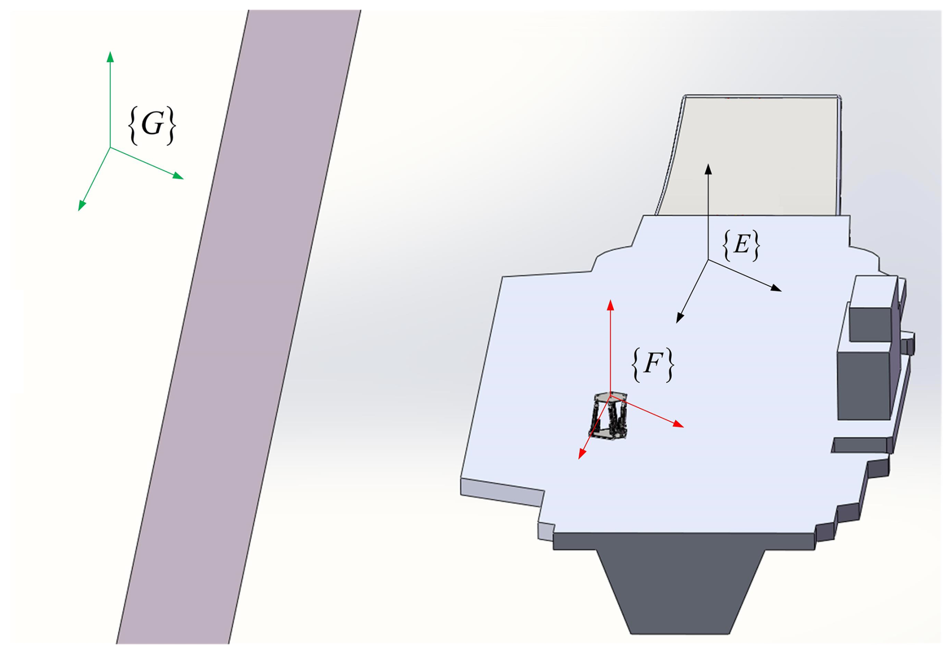
(1.) Multibody reference frames (Fig. 1) were defined as

$$\begin{array}{ll}{\displaystyle }& {\displaystyle }\mathit{\left\{}G\mathit{\right\}}-\text{Earth-fixed inertial frame (global reference)},\\ {\displaystyle }& {\displaystyle }\mathit{\left\{}E\mathit{\right\}}-\text{vessel-attached base frame (lower platform)},\\ {\displaystyle }& {\displaystyle }\mathit{\left\{}F\mathit{\right\}}-\text{end-effector frame (upper moving platform)}.\end{array}$$

Figure 1 Schematic diagram of the reference systems of the shipborne stabilized platform.

(2.) Coordinate transformations between frames were constructed using

$$\begin{array}{}\text{(1)}& {\mathit{P}}_G={\mathit{R}}_G^E\left({\mathrm{\Theta }}_{\text{EV}}\right)\left({\mathit{P}}_E+{\mathit{R}}_E^F\left({\mathrm{\Theta }}_{\text{FP}}\right){\mathit{p}}_F\right)+{\mathit{t}}_G^E,\end{array}$$

where P_G is the absolute position in {G}, ${\mathit{R}}_G^E\in \text{SO}\left(\mathrm{3}\right)$ is the vessel-to-Earth rotation matrix ($\text{RPY\hspace{0.17em}\hspace{0.17em}angles}{\mathrm{\Theta }}_{\text{EV}}=[\mathit{\varphi },\mathit{\theta },\mathit{\psi }{]}^{\mathrm{T}}$), ${\mathit{R}}_E^F\in \text{SO}\left(\mathrm{3}\right)$ is the platform-to-vessel rotation matrix $({\mathrm{\Theta }}_{\text{FP}}=[\mathit{\alpha },\mathit{\beta },\mathit{\gamma }{]}^{\mathrm{T}})$, and ${\mathit{t}}_G^E$ is the translation vector from {G} to {E} origin.

(3.) Critical parameters, including geometric dimensions and mass properties, are listed in Table 1, and the coordinate relationship symbols are systematically defined in Table 2.

As shown in Fig. 2 for the distribution of the hinge position of each key connection point of the shipborne stabilized platform, the position of the origin of the {F} coordinate system under the {E} coordinate system is ${}^E{O}_F=\left({}^E{O}_{Fx}^E{O}_{Fy}^E{O}_{Fz}\right)$.

Table 1 Key design parameters of the 6-DOF parallel platform.

Figure 2 Distribution diagram of the main hinge points of the shipborne stabilized platform.

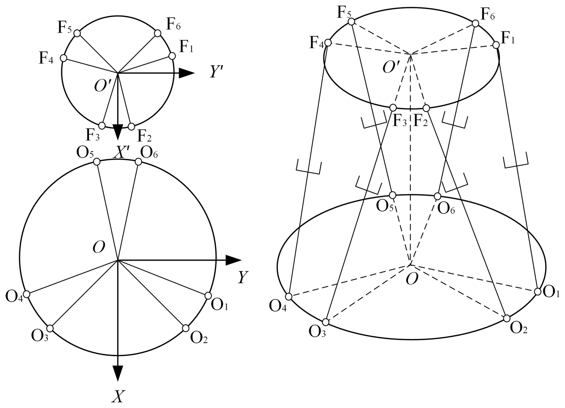
Table 2 Symbol definitions and coordinate relationships.

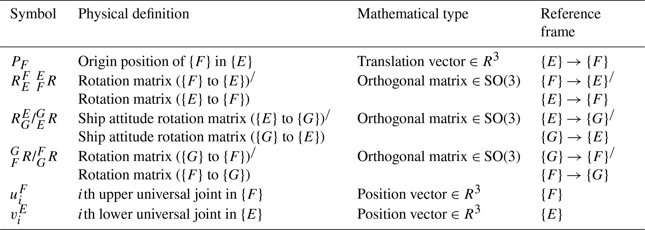
Note: All coordinate systems follow the right-hand rule. Rotation matrices comply with ${\mathit{R}}^{\mathrm{T}}={\mathit{R}}^{-\mathrm{1}}$.

The position of the upper platform center of mass in {F} is {^FC_up} and its position under the {E} system is {^EC_up}, which can be calculated by

$$\begin{array}{}\text{(2)}& {}^E{C}_{\text{up}}={}^E{O}_F+{}_F^E\mathit{R}{}^F{C}_{\text{up}}.\end{array}$$

The distribution of the hinge nodes of the shipborne stabilized platform is shown in Fig. 3. The position of the ith hinge point of the upper platform under the {F} coordinate system can be expressed as ^FS_i=(^FS_ix^FS_iy^FS_iz)^T. The position of the ith hinge point of the platform on the shipborne stabilized platform can then be expressed in the {E} coordinate system by

$$\begin{array}{}\text{(3)}& {}^E{S}_i={}^E{O}_F+{}_F^E\mathit{R}{}^F{S}_i.\end{array}$$

Figure 3 The figure of the fixed-attitude workspace solution results.

The position of the gimbal center point of the ith leg of the lower platform in the {E} coordinate system can be expressed as ^EU_i=(^EU_ix^EU_iy^EU_iz)^T. The ith leg length vector is ${\mathit{J}}_i^{\text{ac}}$, which is obtained by solving for its upper gimbal center and lower gimbal center points in the {E} coordinate system.

$$\begin{array}{}\text{(4)}& {}^E{\mathit{J}}_i^{\text{ac}}={}^E{S}_i-{}^E{U}_i\end{array}$$

From the above rotation matrix, we obtain

$$\begin{array}{}\text{(5)}& {}_F^G\mathit{R}={}_E^G\mathit{R}{}_F^E\mathit{R}.\end{array}$$

2.1.1 Kinematic modeling in non-inertial systems

In comparison with the previous section, the {E} coordinate system is a local coordinate system that moves with the inertial coordinate system. Thus, the center-of-mass position of the platform on the shipborne stabilized platform in the {G} coordinate system is as follows:

$$\begin{array}{}\text{(6)}& {}^G{C}_{\text{up}}={}^G{O}_E+{}_E^G\mathit{R}{}^E{O}_F+{}_E^G\mathit{R}{}_F^E\mathit{R}{}^F{C}_{\text{up}},\end{array}$$

where ^GO_E represents the coordinate position of the origin of the {E} coordinate system in the {G} coordinate system and ^EC_up represents the position of the upper platform under the {E} coordinate system. The solution based on the above positions' yields the following:

$$\begin{array}{}\text{(7)}& {}^G{C}_{\text{up}}={}^G{O}_E+{}_E^G\mathit{R}{}^E{C}_{\text{up}}.\end{array}$$

Both sides of Eq. (7) are differentiated to first order in time, and the velocity of the center of mass of the upper platform in the {G} coordinate system is solved as follows:

$$\begin{array}{}\text{(8)}& {}^G{\dot{C}}_{\text{up}}={}^G{\dot{O}}_E+{}_E^G\mathit{R}{}^E{C}_{\text{up}}\times {}_E^G\mathit{\omega }+{}_E^G\mathit{R}{}^E{\dot{C}}_{\text{up}},\end{array}$$

where ${}^G{\dot{O}}_E$ represents the velocity of the origin of the {E} coordinate system in the {G} coordinate system, ${}_E^G\dot{\mathit{\omega }}$ represents the angular velocity of the {E} coordinate system in the {G} coordinate system, and ${}^E{\dot{C}}_{\text{up}}$ represents the velocity of the upper platform under the {E} coordinate system.

Figure 4 The result of the inverse position.

Figure 5 The result of the velocity inverse solution.

The acceleration of the center of mass of the upper platform in the {G} coordinate system is solved by second-order differentiation against time on both sides:

$$\begin{array}{}\text{(9)}& \begin{array}{rl}{}^G{\ddot{C}}_{\text{up}}=& {}^G{\ddot{O}}_E+{}_E^G\mathit{R}{}^E{C}_{\text{up}}\times {}_E^G\dot{\mathit{\omega }}+\left({}_E^G\mathit{R}{}^E{C}_{\text{up}}\times {}_E^G\mathit{\omega }\right)\\ & \times {}_E^G\mathit{\omega }+\mathrm{2}{}_E^G\mathit{\omega }\times {}_E^G\mathit{R}{}^E{\dot{C}}_{\text{up}}+{}_E^G\mathit{R}{}^E{\ddot{C}}_{\text{up}},\end{array}\end{array}$$

where ${}^G{\ddot{O}}_E$ represents the acceleration of the origin of the {E} coordinate system in the {G} coordinate system and ${}_E^G\dot{\mathit{\omega }}$ represents the angular acceleration of the {E} coordinate system in the {G} coordinate system. The angular velocity of the upper platform in the {G} coordinate system, i.e., the angular velocity of the {F} coordinate system in the {G} coordinate system, is as follows:

$$\begin{array}{}\text{(10)}& {}_F^G\mathit{\omega }={}_E^G\mathit{\omega }+{}_E^G\mathit{R}{}_F^E\mathit{\omega }.\end{array}$$

The angular acceleration of the upper platform in the {G} coordinate system is solved for both sides of Eq. (10) for first-order differentiation in time:

$$\begin{array}{}\text{(11)}& {}_F^G\dot{\mathit{\omega }}={}_E^G\dot{\mathit{\omega }}+{}_E^G\mathit{\omega }{}_E^G\mathit{R}{}_F^E\mathit{\omega }+{}_E^G\mathit{R}{}_F^E\dot{\mathit{\omega }},\end{array}$$

where ${}_F^G\dot{\mathit{\omega }}$ represents the angular acceleration of the center of mass of the upper platform in the {G} coordinate system. The position of the center of the first leg in the {G} coordinate system is as follows:

$$\begin{array}{}\text{(12)}& {}^G{S}_i={}^G{O}_E+{}_E^G\mathit{R}{}^E{S}_i.\end{array}$$

Figure 6 The inverse solution results in acceleration.

The first-order differentiation of time on both sides of Eq. (12) is solved for the velocity of the center of the first leg in the {G} coordinate system:

$$\begin{array}{}\text{(13)}& {}^G{\dot{S}}_i={}^G{\dot{O}}_E+{}_E^G\mathit{\omega }\times {}_E^G\mathit{R}{}^E{S}_i+{}_E^G\mathit{R}{}^E{\dot{S}}_i.\end{array}$$

The acceleration of the center of the ith leg in the {G} coordinate system is solved for the second-order differentiation of time on both sides of Eq. (13):

$$\begin{array}{}\text{(14)}& \begin{array}{rl}{}^G{\ddot{S}}_i=& {}^G{\ddot{O}}_E+{}_E^G\dot{\mathit{\omega }}\times {}_E^G\mathit{R}{}^E{S}_i+{}_E^G\mathit{\omega }\times \left({}_E^G\mathit{R}{}^E{S}_i\times {}_E^G\mathit{\omega }\right)\\ & +{}_E^G\mathit{R}{}^E{\ddot{S}}_i+\mathrm{2}{}_E^G\mathit{\omega }\times {}_E^G\mathit{R}{}^E{\dot{S}}_i.\end{array}\end{array}$$

The position of the piston center of mass in the ith leg in the {G} coordinate system is as follows:

$$\begin{array}{}\text{(15)}& {}^G{r}_{i\mathrm{u}}={}^G{O}_E+{}_E^G\mathit{R}{}^E{r}_{i\mathrm{u}}.\end{array}$$

The first-order differentiation of time on both sides of Eq. (15) is solved for the velocity of the piston center of mass of the first leg in the {G} coordinate system:

$$\begin{array}{}\text{(16)}& {}^G{\dot{r}}_{i\mathrm{u}}={}^G{\dot{O}}_E+{}_E^G\mathit{\omega }\times {}_E^G\mathit{R}{}^E{r}_{i\mathrm{u}}+{}_E^G\mathit{R}{}^E{\dot{r}}_{i\mathrm{u}}.\end{array}$$

The angular velocity of the ith leg of the shipborne stabilized platform in the {G} coordinate system ${}_{Q_i^G}\mathit{\omega }$ is solved as follows:

$$\begin{array}{}\text{(17)}& {}_{Q_i^G}\mathit{\omega }={}_E^G\mathit{\omega }+{}_E^G\mathit{R}{}_{Q_i^E}\mathit{\omega }.\end{array}$$

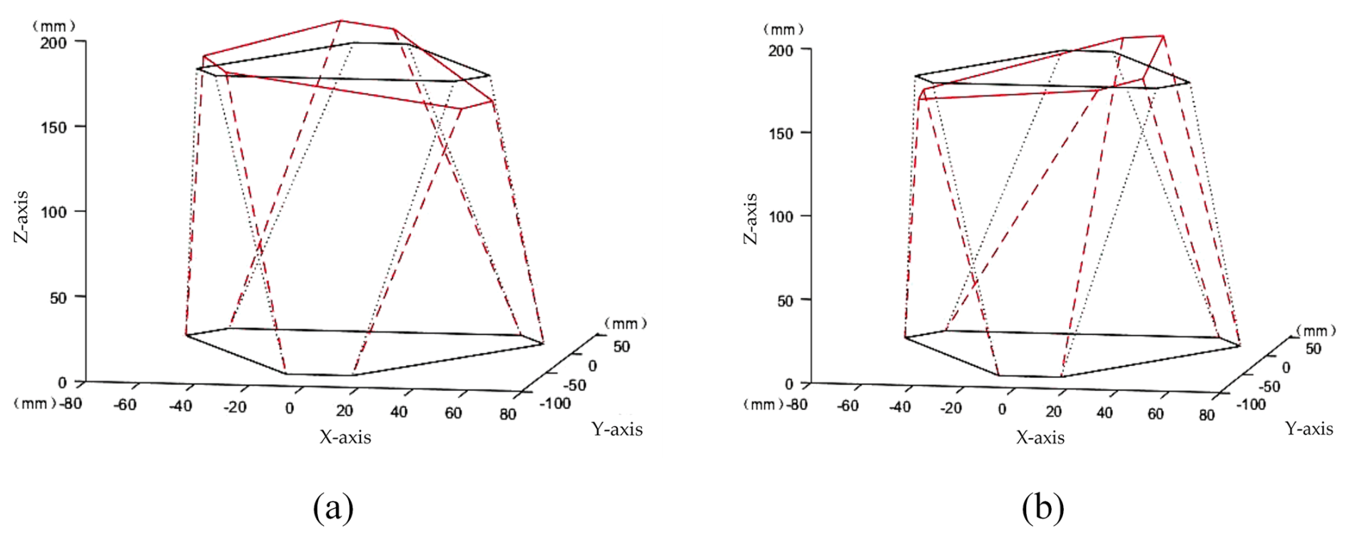
Figure 7 Output space and initial position comparison diagram: (a) output posture example 1; (b) output posture example 2.

The angular velocity ${}_{Q_i^G}\dot{\mathit{\omega }}$ of the ith leg in the {G} coordinate system is solved for both sides of Eq. (17) for first-order differentiation in time:

$$\begin{array}{}\text{(18)}& {}_{Q_i^G}\dot{\mathit{\omega }}={}_E^G\dot{\mathit{\omega }}+{}_E^G\mathit{R}{}_{Q_i^E}\mathit{\omega }\times {}_E^G\mathit{\omega }+{}_E^G\mathit{R}{}_{Q_i^E}\dot{\mathit{\omega }}.\end{array}$$

The acceleration of the piston center of mass of the ith leg in the {G} coordinate system is solved for the first-order differentiation of time on both sides of Eq. (16):

$$\begin{array}{}\text{(19)}& \begin{array}{rl}{}^G{\ddot{r}}_{i\mathrm{u}}=& {}^G{\ddot{O}}_E+{}_E^G\mathit{R}{}^E{\ddot{r}}_{i\mathrm{u}}+{}_E^G\dot{\mathit{\omega }}\times {}_E^G\mathit{R}{}^E{r}_{i\mathrm{u}}+{}_E^G\mathit{\omega }\\ & \times \left({}_E^G\mathit{\omega }\times {}_E^G\mathit{R}{}^E{r}_{i\mathrm{u}}\right)+\mathrm{2}{}_E^G\mathit{\omega }\times {}_E^G\mathit{R}{}^E{\dot{r}}_{i\mathrm{u}}.\end{array}\end{array}$$

The position of the cylinder center of mass at the ith branch angle in the {G} coordinate system is as follows:

$$\begin{array}{}\text{(20)}& {}^G{r}_{i\mathrm{l}}={}^G{O}_E+{}_E^G\mathit{R}{}^E{r}_{i\mathrm{l}}.\end{array}$$

Both sides of Eq. (20) are differentiated to the first order in time, and the velocity of the cylinder center of mass of the ith leg in the {G} coordinate system is solved as follows:

$$\begin{array}{}\text{(21)}& {}^G{\dot{r}}_{i\mathrm{l}}={}^G{\dot{O}}_E+{}_E^G\mathit{\omega }\times {}_E^G\mathit{R}{}^E{r}_{i\mathrm{l}}+{}_E^G\mathit{R}{}^E{\widehat{r}}_{i\mathrm{l}}.\end{array}$$

The acceleration of the cylinder center of mass of the ith leg in the {G} coordinate system is solved for the second-order differentiation of time on both sides of Eq. (21):

$$\begin{array}{}\text{(22)}& \begin{array}{rl}{}^G{\ddot{r}}_{i\mathrm{l}}=& {}^G{\ddot{O}}_E+{}_E^G\dot{\mathit{\omega }}\times {}_E^G\mathit{R}{}^E{r}_{i\mathrm{l}}+{}_E^G\mathit{\omega }\times \left({}_E^G\mathit{\omega }\times {}_E^G\mathit{R}{}^E{r}_{i\mathrm{l}}\right)\\ & +{}_E^G\mathit{R}{}^E{\ddot{r}}_{i\mathrm{l}}+\mathrm{2}{}_E^G\mathit{\omega }\times {}_E^G\mathit{R}{}^E{\dot{r}}_{i\mathrm{l}}.\end{array}\end{array}$$

2.1.2 Workspace parameter analysis

In this paper, a stochastic probabilistic algorithm based on a numerical method, the Monte Carlo simulation method, is used. It is particularly noteworthy that the error of this method is not associated with the dimensionality of its system and can be solved directly for problems containing statistical properties in the system, while no discretization is required for continuous problems (Hunek et al., 2022; Jing et al., 2024).

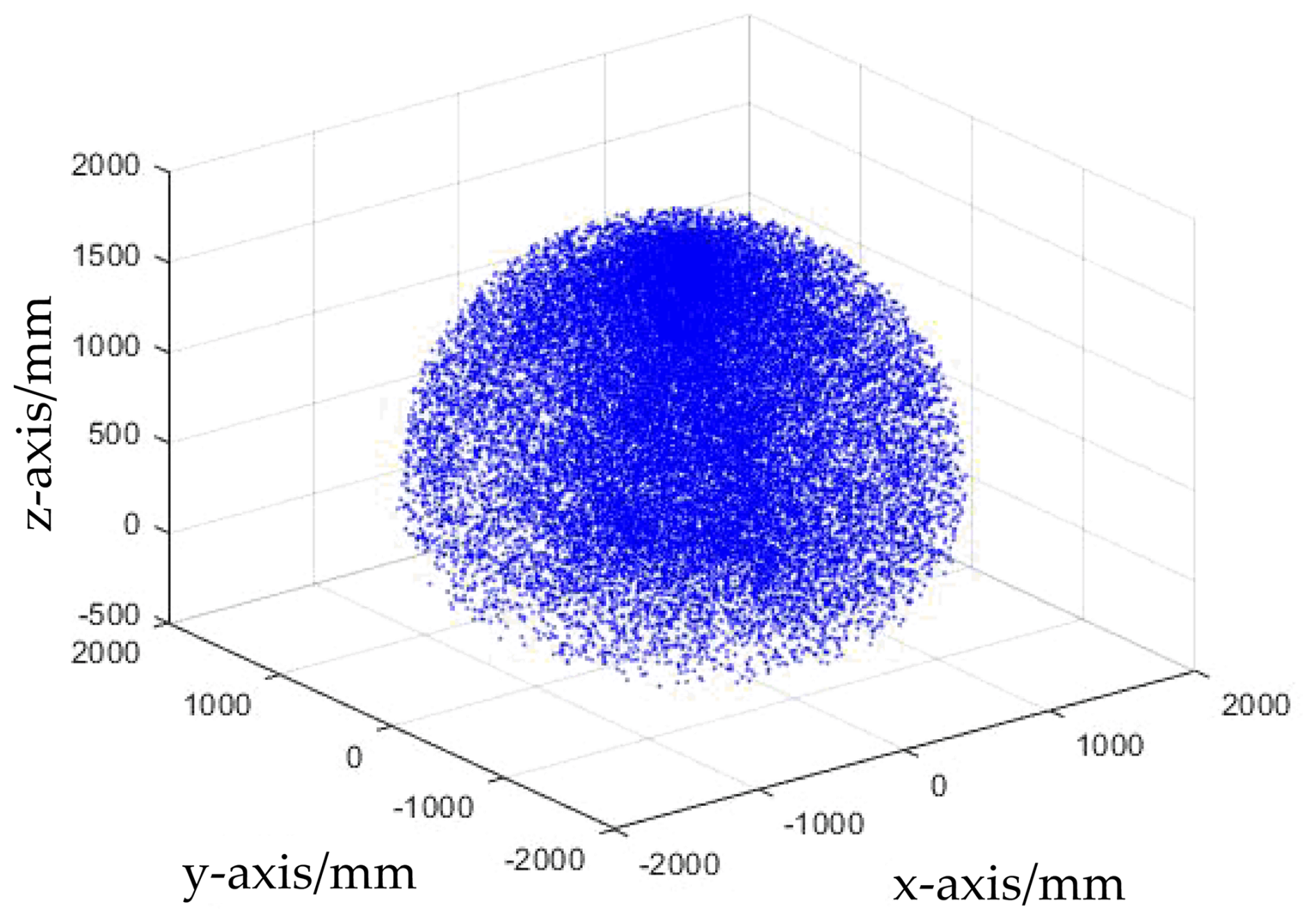
For the randomness of the Monte Carlo method, we use the rand () function for the representation, followed by the random number selection of the joint angles of the shipborne stabilized platform in its angle range. The code is as follows: $\mathit{\theta }min\times (\mathit{\pi }/\mathrm{180})+(\mathit{\theta }max-\mathit{\theta }min)\times (\mathit{\pi }/\mathrm{180})\times \text{rand}$. The meaning of this code is as follows: taking the angle range as the minimum value is used as the basis, and the random number in the angle range is added to get the current joint random value of this axis. Finally, the end position is obtained by the kinematic script and plotted by the plot3() function to obtain the approximate workspace. The number of steps set in this practical example is 40 000, whether it is a scatterplot or an indicator of the workspace, the accuracy of which depends on the pre-set step size. The Monte Carlo simulation method is more convenient for the spatial evaluation of the workspace, as shown in Fig. 3 for the graph of the results of this fixed-attitude workspace solution.

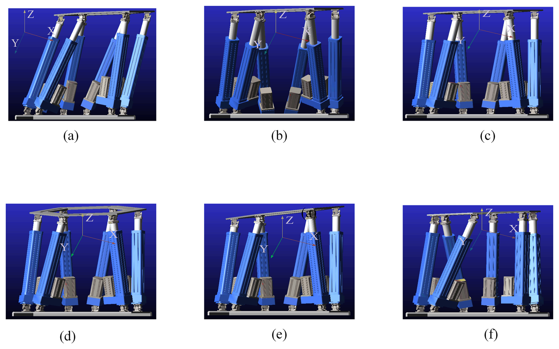
Figure 8 Realization of the 6-DOF shipborne stabilized platform. The required degrees of freedom are obtained as follows: (a) translate in the X direction, (b) translate in the Y direction, (c) translate in the Z direction, (d) rotate around the X axis, (e) rotate around the Y axis, and (f) rotate around the Z axis.

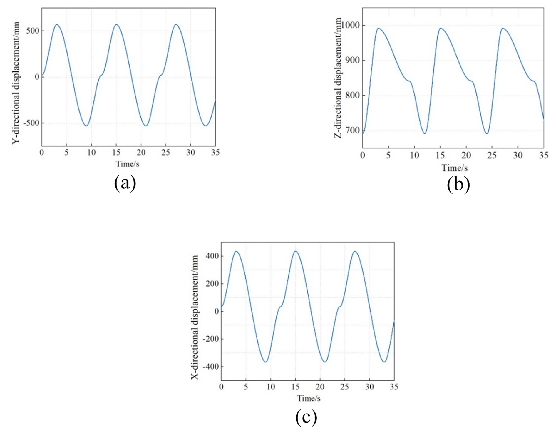
Figure 9 Motion curve of the upper platform: (a) X-directional displacement; (b) Y-directional displacement; (c) Z-directional displacement.

2.1.3 Stabilized platform parametric interface simulation

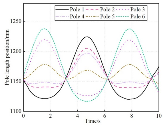
Based on the above kinematic model of the shipborne stabilized platform, the simulation program is established, and the parametric motion simulation of the shipborne stabilized platform is realized through the user interface. The parameters of the stabilized platform are input, including the outer circumferential radius of the platform and the distribution angle of the platform hinge point; the motion trajectory of the platform is filled in; and the position of the inverse solution to get the rod length position curve and data of the platform is selected. The inverse solution results are shown in Fig. 4.

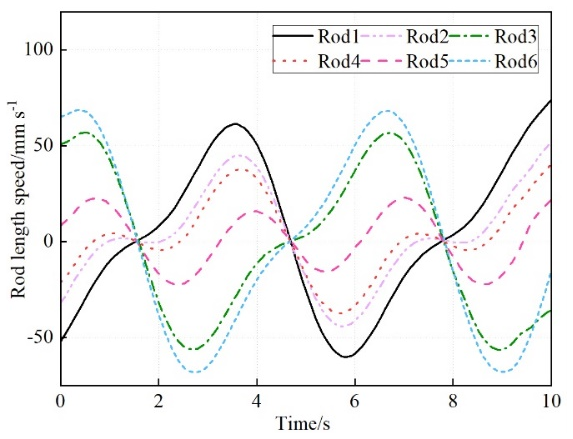
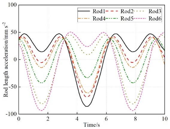
Similarly, by inputting the machine parameters and motion trajectory and then selecting the velocity inverse solution, the rod length velocity curve and data of the drive joint can be obtained; these output results are shown in Fig. 5. After inputting the parameters and selecting the acceleration inverse solution, the rod length acceleration curve and data of the drive mechanism can be obtained; these output results are shown in Fig. 6.

For an input yaw angle of 15°, a pitch angle of 20°, and a roll angle of 25°, the output spatial position compared with the initial position is shown in Fig. 7a. For an input yaw angle of −5°, a pitch angle of −15°, and a roll angle of −10°, the output spatial position compared with the initial position is shown in Fig. 7b.

Figure 10 Dynamics simulation curve.

Figure 11 A control subsystem module.

2.2 Kinetic analysis

Based on D'Alembert's theorem, the inertial force acting on each moving part of the platform on the shipborne stabilized platform can be expressed as

$$\begin{array}{}\text{(23)}& f_{\mathrm{u}}=-m_{\mathrm{u}}{}^G{\ddot{C}}_{\mathrm{u}},\end{array}$$

where m_u represents the mass of the platform on the shipborne stabilized platform.

The gravitational force applied to the upper platform can be expressed as

$$\begin{array}{}\text{(24)}& G_{\mathrm{u}}=m_{\mathrm{u}}g,\end{array}$$

where g represents the acceleration of gravity.

The upper-platform inertia force can be expressed as

$$\begin{array}{}\text{(25)}& M_{\mathrm{u}}=-{}^G{I}_{\mathrm{u}}{}_F^G\dot{\mathit{\omega }}-{}_F^G\mathit{\omega }\times \left({}^G{I}_{\mathrm{u}}{}_F^G\mathit{\omega }\right),\end{array}$$

where ^FI_u represents the inertia tensor of the upper platform at {G}.

$$\begin{array}{}\text{(26)}& {}^G{I}_{\mathrm{u}}={}_F^G\mathit{R}{}^F{I}_{\mathrm{u}}{}_G^F\mathit{R},\end{array}$$

where ^FI_u represents the inertia tensor of the upper platform at {F}, ${}_G^F\mathit{R}={}_F^G{\mathit{R}}^{\mathrm{T}}$. The inertia force of the ith leg piston is as follows:

$$\begin{array}{}\text{(27)}& f_{i\mathrm{u}}=-m_{i\mathrm{u}}{}^G{\ddot{r}}_{i\mathrm{u}},\end{array}$$

where m_iu denotes the mass of the ith foot piston.

The gravity of the ith leg piston can be expressed as

$$\begin{array}{}\text{(28)}& G_{i\mathrm{u}}=m_{i\mathrm{u}}g.\end{array}$$

The moment of inertia of the ith leg piston can be expressed as

$$\begin{array}{}\text{(29)}& M_{i\mathrm{u}}=-{}^G{I}_{i\mathrm{u}}{{}_{Q_i}}^G\dot{\mathit{\omega }}-{{}_{Q_i}}^G\mathit{\omega }\times \left({}^G{I}_{i\mathrm{u}}{{}_{Q_i}}^G\mathit{\omega }\right),\end{array}$$

where ^GI_iu represents the inertia tensor of the ith foot piston at {G}.

$$\begin{array}{}\text{(30)}& {}^G{I}_{i\mathrm{u}}={{}_{Q_i}}^G\mathit{R}{}^{Q_i}{I}_{i\mathrm{u}}{}_G^{Q_i}\mathit{R},\end{array}$$

where ${}^{Q_i}{I}_{i\mathrm{u}}$ represents the inertia tensor of the first leg piston under {Q_i} and ${}_G^{Q_i}\mathit{R}$ represents the rotation matrix from {G} to {Q_i} (${}_G^{Q_i}\mathit{R}={{}_{Q_i}}^G{\mathit{R}}^{\mathrm{T}}$).

The inertia force of the ith leg cylinder is as follows:

$$\begin{array}{}\text{(31)}& f_{i\mathrm{l}}=-m_{i\mathrm{l}}{}^G{\ddot{r}}_{i\mathrm{l}},\end{array}$$

where m_il represents the moment of inertia of the ith leg cylinder.

$$\begin{array}{}\text{(32)}& M_{i\mathrm{l}}=-{}^G{I}_{i\mathrm{l}}{{}_{Q_i}}^G\dot{\mathit{\omega }}-{{}_{Q_i}}^G\mathit{\omega }\times \left({}^G{I}_{i\mathrm{l}}{{}_{Q_i}}^G\mathit{\omega }\right),\end{array}$$

where ^GI_il represents the inertia tensor of the ith foot sleeve under {G}.

$$\begin{array}{}\text{(33)}& {}^G{I}_{i\mathrm{u}}={{}_{Q_i}}^G\mathit{R}{}^{Q_i}{I}_{i\mathrm{u}}{}_G^{Q_i}\mathit{R},\end{array}$$

where ${}^{Q_i}{I}_{i\mathrm{u}}$ represents the inertia tensor of the ith leg under the cylinder.

Figure 12 Input and output.

2.3 Platform performance analysis

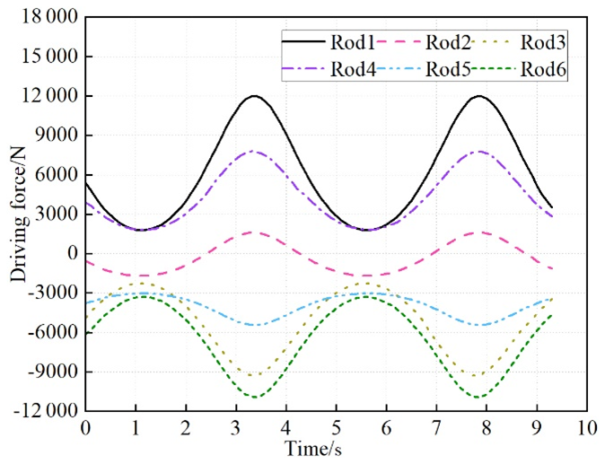
The experimental framework established 12 gimbal centers as coordinate origins, with corresponding components systematically integrated: gimbal vices positioned at each pivot node, cylindrical joints connecting motion rods to outer rails, and a central-point drive mechanism mounted on the upper platform (Fig. 8). Parameter initialization involved a two-phase simulation protocol – commencing with a 35 s dynamic analysis encompassing 4000 computational steps for platform trajectory validation, followed by a 9.36 s precision simulation executing 982 discrete steps for actuator force quantification. The implemented drive functions demonstrated 6-DOF motion compliance (Fig. 9) and enabled directional vector analysis of actuator forces (Fig. 10).

Simulation outcomes substantiated the virtual prototype's efficacy through three critical performance indicators: rapid response capability, evidenced by sub-15 s motion cycle completion across all translational axes (Fig. 9); smooth force transitions, maintaining continuous derivative profiles in all actuators (Fig. 10); operational stability, demonstrated by force curves exhibiting monotonic variation patterns. This validation establishes reliable foundational support for marine stabilization platform co-simulation studies, confirming effective coordination between dynamic responsiveness and operational steadiness.

3 Joint simulation and system design

Based on the virtual-prototype model of the shipboard stabilization platform established above, data exchange of state variables is performed to realize the joint simulation and analyze the system at the same time.

3.1 Construction of the co-simulation module

The co-simulation process of the shipborne stabilized platform is divided into three steps. The first is model building, which consists of three main aspects: geometry modeling, element division, and attribute definition. Secondly, the input and output interfaces of the built model are set up, determining the inputs and outputs. Finally, the simulation parameters are set to carry out the joint simulation, plot the simulation curves, and solve the simulation results.

3.2 Design of the control programs

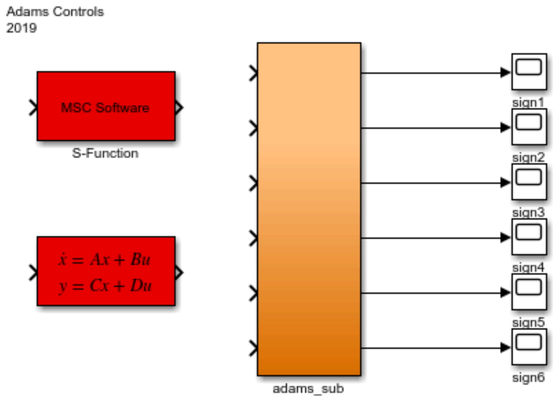
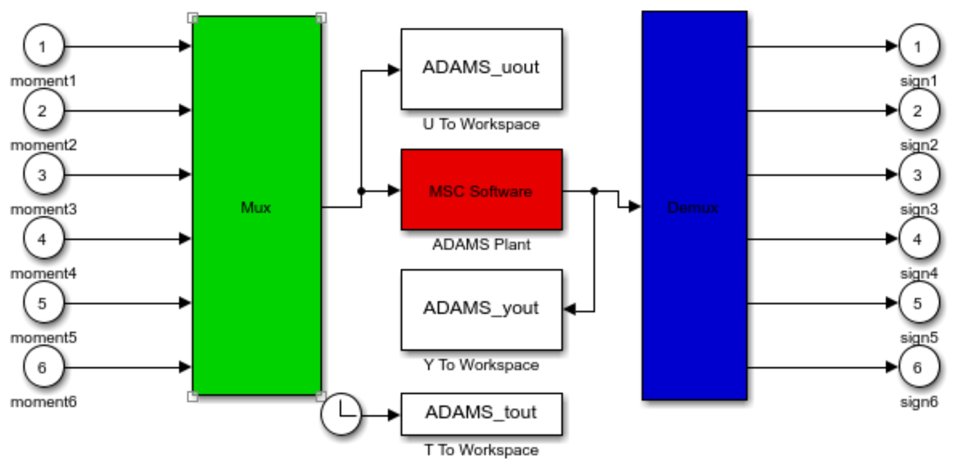
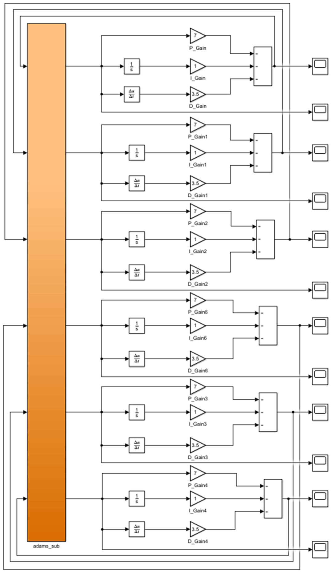
The model is first initialized with parameters, and the simulation software is then interconnected, as shown in the selection window of Simulink in Fig. 11. The S-Function module encapsulates the nonlinear model of the shipborne stabilized platform developed in the previous section, while the State-Space module specifically refers to the linearized state–space representation derived from the original nonlinear multibody dynamics model through ADAMS-software-based linearization. This linearized model serves two critical purposes:

1. simplify the controller design by reducing model complexity;

2. enable joint simulation verification, particularly under conditions involving small disturbances.

The Adams_sub module contains the complete nonlinear equations and associated variables, with the S-Function module providing the interface for co-simulation. As shown in Fig. 12, this dual-model architecture integrates both representations to achieve a comprehensive dynamic analysis capability.

In the co-simulation, traditional frequency-domain analysis methods based on transfer functions (e.g., Bode plots and root locus) are challenging to apply directly, due to the nonlinear multibody dynamics model of the platform (ADAMS–Simulink coupling). Consequently, the initial PID parameter tuning adheres to a stability-first principle, employing empirical tuning methods: the baseline proportional gain is determined through the Ziegler–Nichols critical gain method based on step response characteristics, while integral and derivative times are fine-tuned through trial and error to balance dynamic response speed and overshoot suppression.

The PID parameters in Fig. 13 were optimized through Ziegler–Nichols tuning and fuzzy adaptation, governed by motor constants, control laws, hierarchical refinements, and results.

Table 3 Fuzzy control table of ΔK_p.

Table 4 Fuzzy control table of ΔK_i.

Table 5 Fuzzy control table of ΔK_d.

Motor constants were as follows: K_e = 2.75 N m A⁻¹, R_a = 9.5 Ω, T_a=1.3 ms, K_m = 1.52 V (rad s)⁻¹, and T_m = 0.69 s.

Control laws were as follows: K_p⋅sign(e), $K_{\mathrm{i}}\cdot \int \text{sign}\left(e\right)\mathrm{d}t$, and K_d⋅d[sign(e)]dt.

Figure 13 PID control scheme diagram.

Hierarchical refinements were as follows:

1. baseline from Ziegler–Nichols critical gain,

2. dynamic compensation via $T_{\mathrm{m}}/K_{\mathrm{m}}$ = 0.454 s² rad⁻¹,

3. 49-rule fuzzy matrices ($\mathrm{7}\times \mathrm{7}\text{error}/\text{error}-\text{rate}$).

Results were as follows: a settling time of 0.83 s (1.2T_m) under a $K_{\mathrm{e}}/R_{\mathrm{a}}$ = 0.29 V A⁻¹ constraint, validated through co-simulation with nonlinear dynamics.

Figure 14 Fuzzy adaptive PID control strategy.

In this system, the dynamic equations of the motor can be expressed as

$$\begin{array}{}\text{(34)}& u=E+i_{\mathrm{a}}{r}_{\mathrm{a}}+L{\displaystyle \frac{\mathrm{d}{i}_{\mathrm{a}}}{\mathrm{d}t}},\end{array}$$

where E represents the induced electromotive force during the dynamic process, u represents the voltage during the dynamic process, i_a represents the current during the dynamic process, and r_a represent armature resistance.

$$\begin{array}{}\text{(35)}& E=C_{\mathrm{e}}n,\end{array}$$

where C_e is the torque constant and n is the rotor speed (rpm).

The electromagnetic torque can be expressed as

$$\begin{array}{}\text{(36)}& T_{\mathrm{e}}=C_{\mathrm{m}}{i}_{\mathrm{a}},\end{array}$$

where C_m represents the electric potential speed ratio at rated excitation.

$$\begin{array}{}\text{(37)}& T_{\mathrm{e}}-T_{\mathrm{L}}={\displaystyle \frac{{\text{GD}}^{\mathrm{2}}}{\mathrm{375}}}{\displaystyle \frac{\mathrm{d}n}{\mathrm{d}t}},\end{array}$$

where GD² represents the flywheel torque of the motor (N m⁻¹) and T_L represents the load torque.

By applying the Laplace transform to the time-domain equations, we can derive the frequency-domain representation of the motor system and, ultimately, obtain its transfer function, which can be expressed as follows:

$$\begin{array}{}\text{(38)}& \begin{array}{rl}G\left(s\right)& ={\displaystyle \frac{C_{\mathrm{m}}/r_{\mathrm{a}}}{T_{\mathrm{1}}s+\mathrm{1}}}\cdot {\displaystyle \frac{r_{\mathrm{a}}/C_{\mathrm{e}}{C}_{\mathrm{m}}}{T_{\mathrm{m}}s+\mathrm{1}}}\cdot {\displaystyle \frac{\mathrm{1}}{s}}\\ & ={\displaystyle \frac{\mathrm{0.66}}{s(\mathrm{0.69}\mathrm{s}+\mathrm{1})(\mathrm{0.0013}\mathrm{s}+\mathrm{1})}},\end{array}\end{array}$$

where T₁ represents the armature circuit electromagnetic time constant and T_m represents the power drag electromechanical time constant. Other values in the above expression are as follows: $C_{\mathrm{m}}=\mathrm{2.75}(N\cdot M/A)$, r_a = 9.5 Ω, T₁ = 1.3 × 10⁻³ s, C_e = 1.52 $\mathrm{V}(\mathrm{rad}{\mathrm{s}}^{-\mathrm{1}}{)}^{-\mathrm{1}}$, and T_m = 0.69 s.

The Ziegler–Nichols method was applied to rectify the initial parameters of the fuzzy controller. T_m = 0.69 s, and the fact that the stabilizing platform itself is heavy indicates that the system has high inertia and responds slowly. Wave disturbances require the platform to respond within milliseconds. A higher K_p value can dramatically increase the sensitivity of the system to errors and shorten the adjustment time. T₁ = 1.3 × 10⁻³s indicates a rapid current response. The error accumulation may cause the integral term to go out of control when the shipboard platform is activated or significantly perturbed. A lower K_i value limits the integration speed and avoids oscillations. High-frequency noises, such as wave impacts and mechanical vibrations, need to be passed through the high K_d fast suppression. The differential action is sensitive to the rate of change in the error and can correct the system behavior in advance.

Based on the Ziegler–Nichols method of calculation and then adjusted for the work requirements of the stabilized flat (the final choice of K_p0 = 20 000, K_i0 = 100, and K_d0 = 260), the corresponding fuzzy subsets are chosen as $[\text{NB},\text{NM},\text{NS},\mathrm{Z},\text{PS},\text{PM},\text{PB}]$. The comparative test in Fig. 19 also verifies the validity of the initial parameter selection.

4 Control optimization and real-time interaction

Based on the joint simulation and system design, the shipboard stabilization platform was first optimized, and the fuzzy PID controller was then designed and simulated to complete the correction of the shipboard stabilization platform control system. Finally, the research results were visualized using Qt Creator front-end software.

Figure 15 System model diagram of fuzzy adaptive PID control.

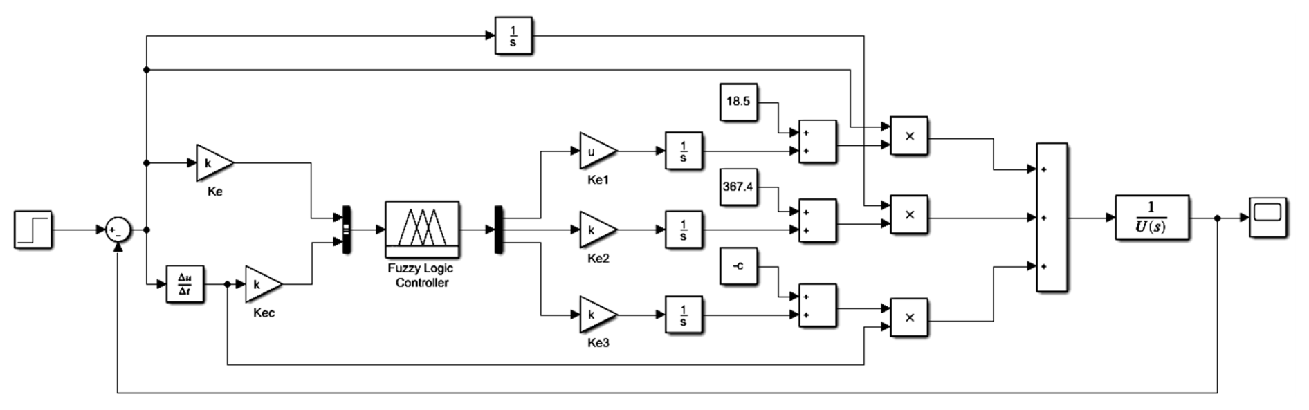
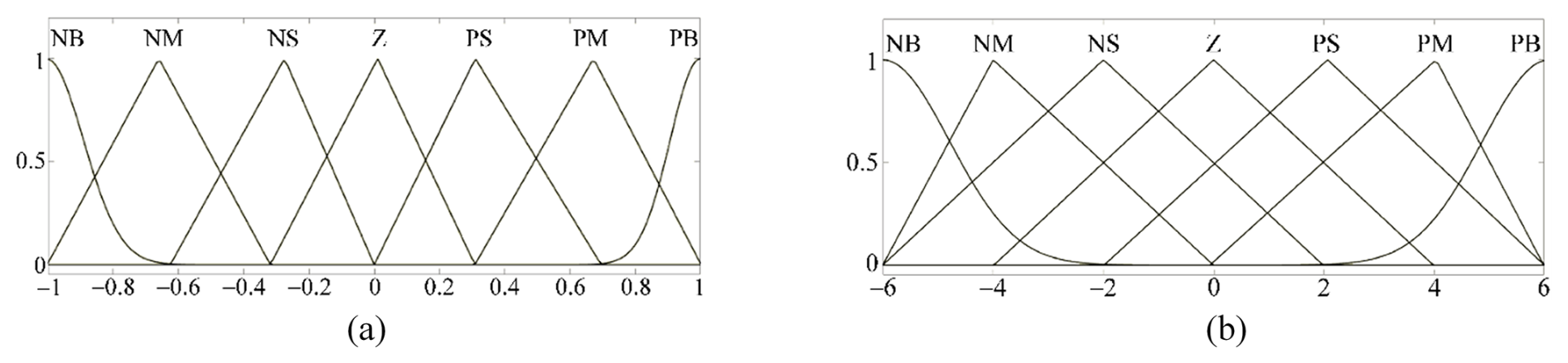
Figure 16 The input membership functions of the fuzzy controller: (a) membership function of the system error e; (b) membership function of the system error change rate ec.

4.1 Fuzzy adaptive PID control design and simulation

The disadvantage of PID control is obvious, the controller parameters are difficult to select (Fan and Teng, 2024). The parameters have a great impact on the performance of the controller, and errors in the parameters may directly lead to system instability and control failure. When encountering nonlinear and strongly coupled systems, the model cannot be recognized, and the parameters cannot be self-regulated or adjusted in real time. Fuzzy adaptive control does not require precise design of the control object and has significant advantages over traditional PID control (Deng et al., 2022). Therefore, the fuzzy adaptive control dynamically adjusts the parameters of the PID controller (Chang et al., 2024) according to the created fuzzy rules in order to make the system more stable and, finally, compares the control effects of the two control methods according to the simulation results.

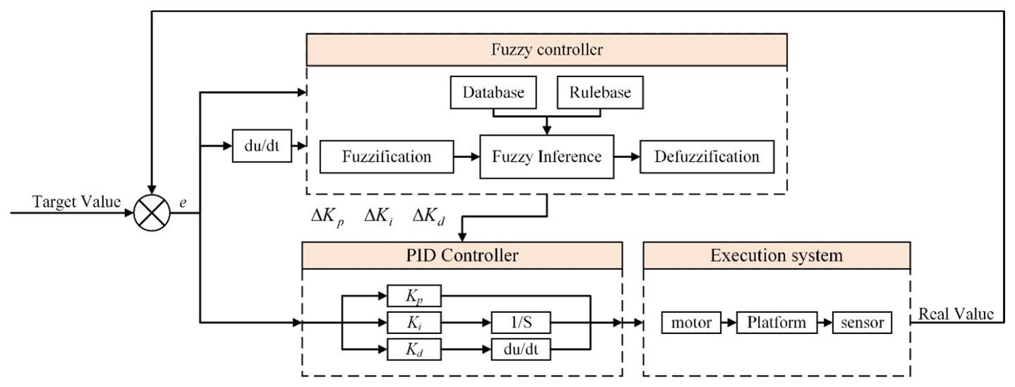
As shown in Fig. 14, in the control strategy of the control system, the platform angle deviation detected by the sensor is recorded as the system error e. The system error e and its change rate ec are used as the inputs of the fuzzy control system and are processed to obtain the quantization factors K_e and K_ec, respectively. K_e and K_ec are fuzzified utilizing the subordinate function library, and fuzzy reasoning is then carried out to obtain the fuzzy outputs according to the control rule library. This is followed by the clarification process, via which we finally obtain the proportional factors ΔK_p, ΔK_i, and ΔK_d, through the proportional factors to the PID control parameters for real-time dynamic adjustment. Finally, according to the fuzzy PID controller output value, the decoupling operation is used to solve the length of each rod, to realize the stabilization and compensation effect on the platform.

4.2 Design of the fuzzy PID controller

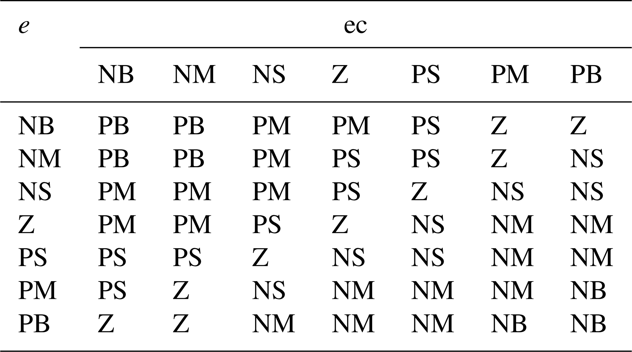
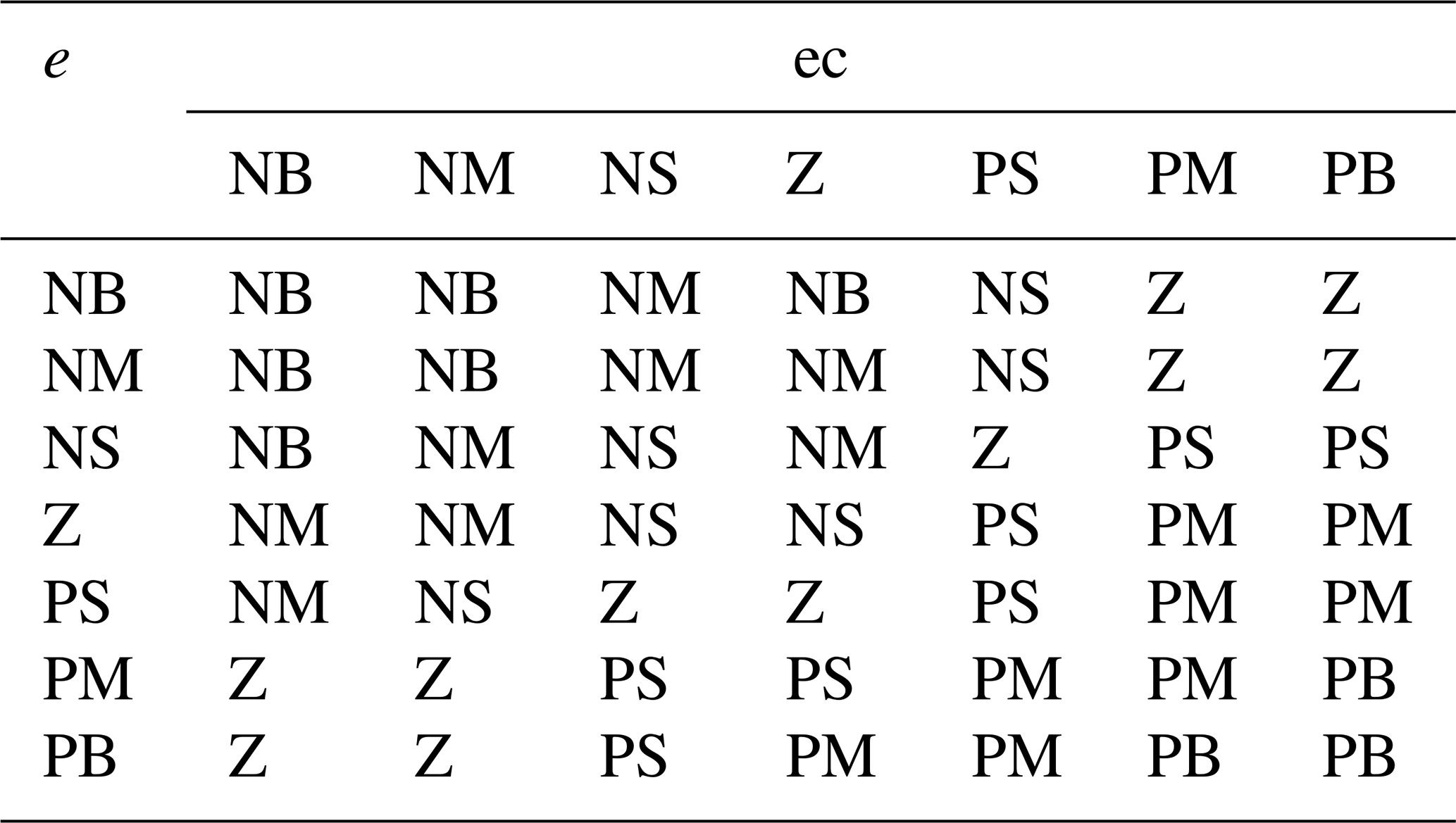
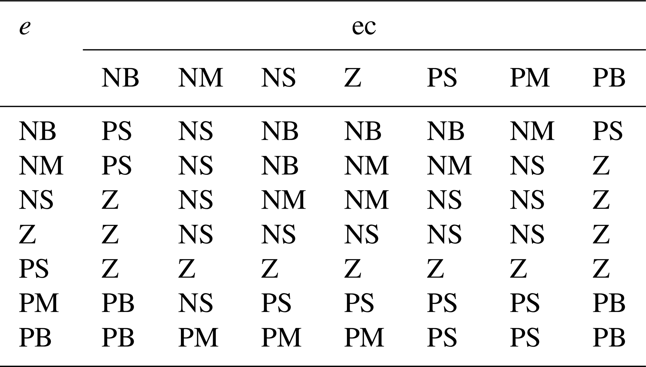
The input variables of the systematic error and its rate of change are determined under the quantization factor. Based on the influence of PID parameters on the system control, the fuzzy rules of ΔK_p, ΔK_i, and ΔK_d are respectively designed by combining the trial-and-error method and the design experience of PID controllers, as shown in Tables 3–5.

With respect to the effect of K_c on the system performance, the larger the K_c, the more the $\mathrm{d}e\left(t\right)/\mathrm{d}t$ interval shrinks and enhances the control effect. Therefore, with a larger selection, the overshoot of the system decreases and the response speed decreases. K_c has a significant effect on the suppression of system overshoot.

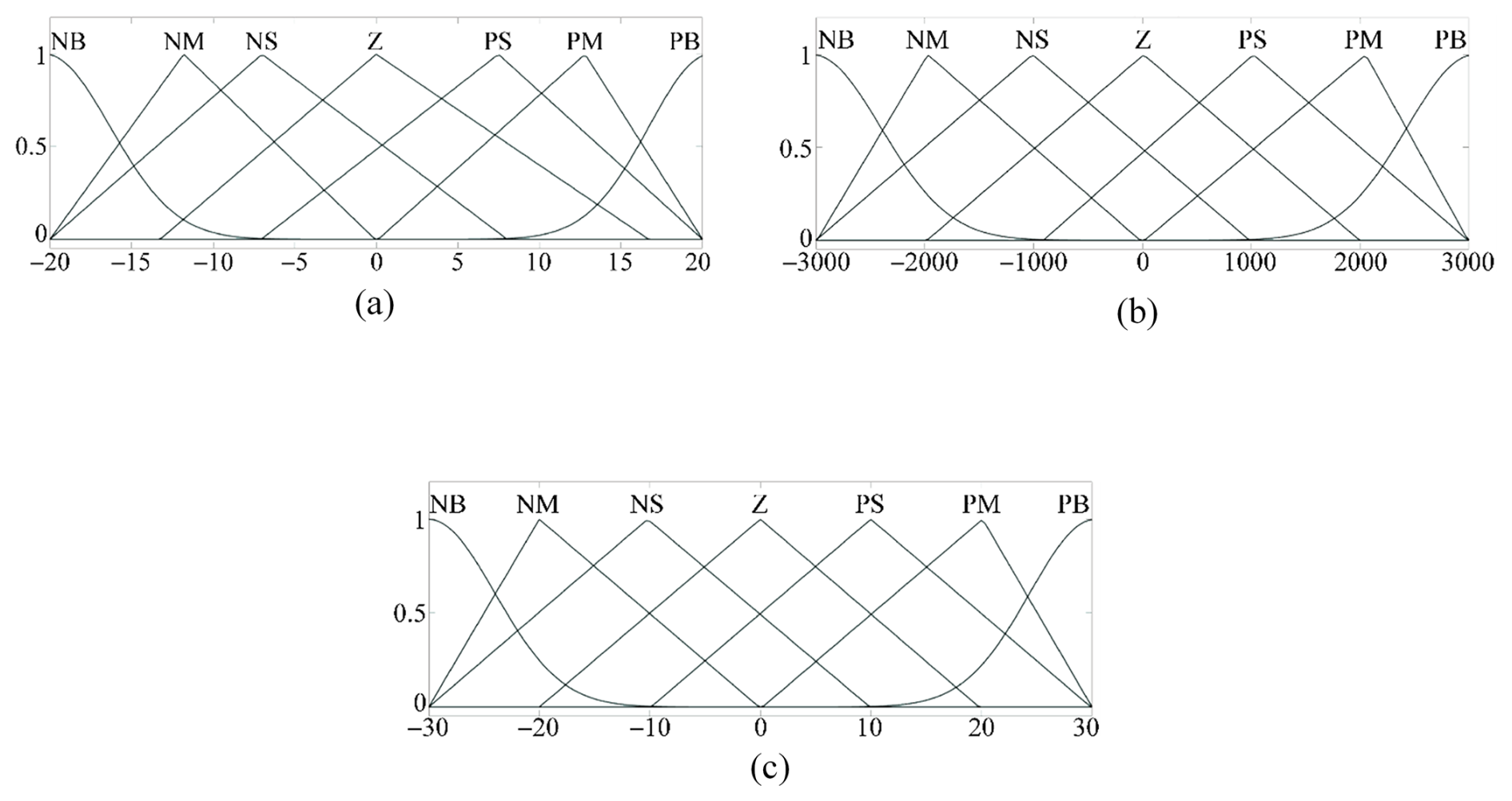
Figure 17 The output membership functions of the fuzzy controller: (a) membership function of the proportional constant ΔK_p; (b) membership function of the integral constant ΔK_i; (c) membership function of the differential constant ΔK_d.

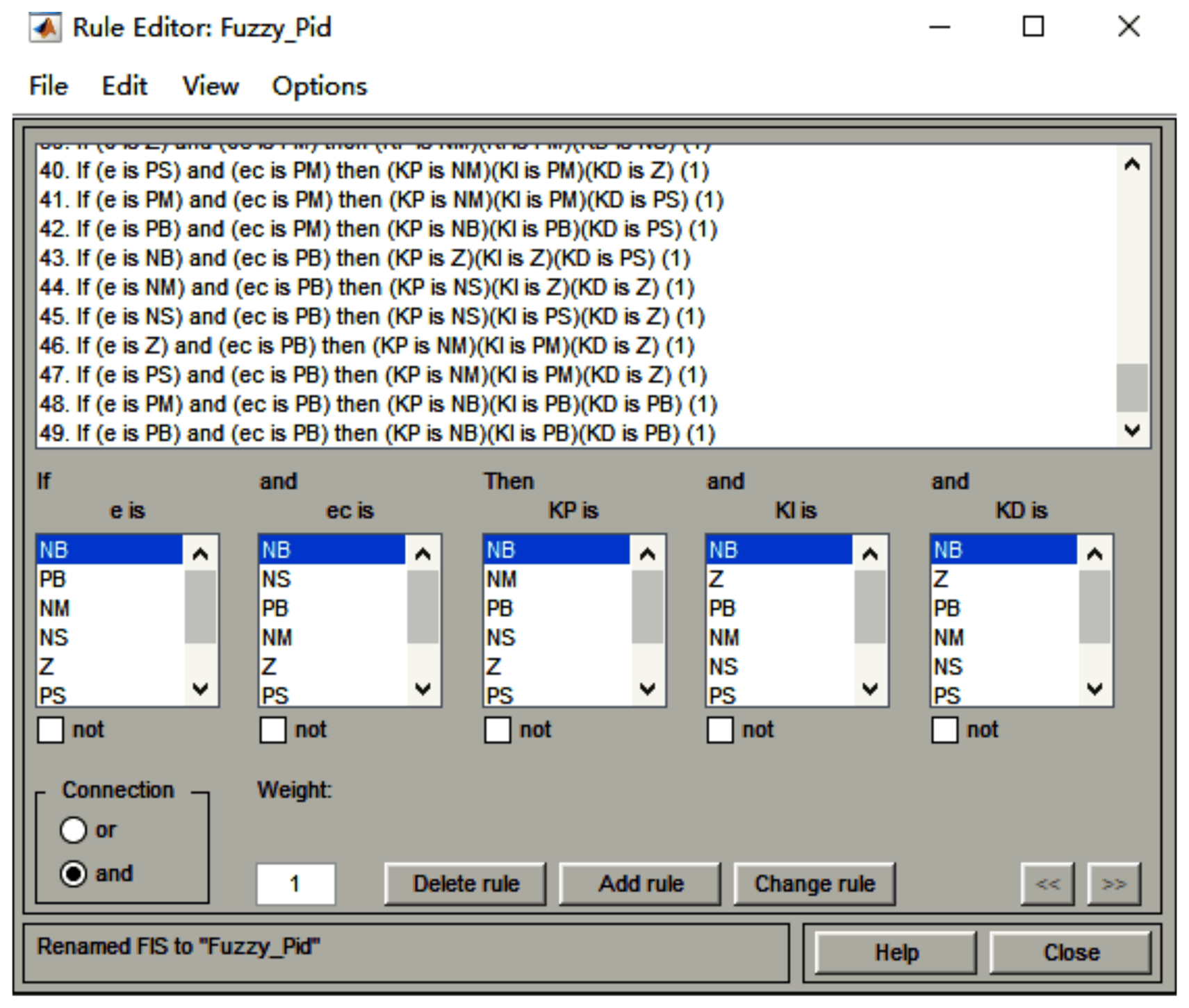
Figure 18 Fuzzy rule editing interface of MATLAB.

The magnitude of K_e greatly affects the dynamic characteristics of the system. The control interval of the fuzzy controller is the interval of variation in the system error e(t) when K_e=1. For K_e<1, the interval of error e(t) expands, leading to a decrease in the sensitivity of the fuzzy controller to the input and, thus, weakening the control of the offset. For K_e>1, the interval of error e(t) contracts, leading to an increase in the sensitivity of the fuzzy controller to the input and, thus, enhancing the control interval of the offset. The rising rate and overshoot of the system increase for larger K_e choices, increasing the transition time. When the output controller output is the same, if K_u is selected to be small, it will lead to a longer dynamic response time of the system. Furthermore, the larger the K_u, the better the controller control effect; the system rings quickly and is easy to overshoot. However, if K_u is selected to be too large, the system produces an oscillation.

Figure 19 Defining inputs and outputs.

Figure 20 Surface relationship of parameters under fuzzy rules: (a) K_p; (b) K_i; (c) K_d.

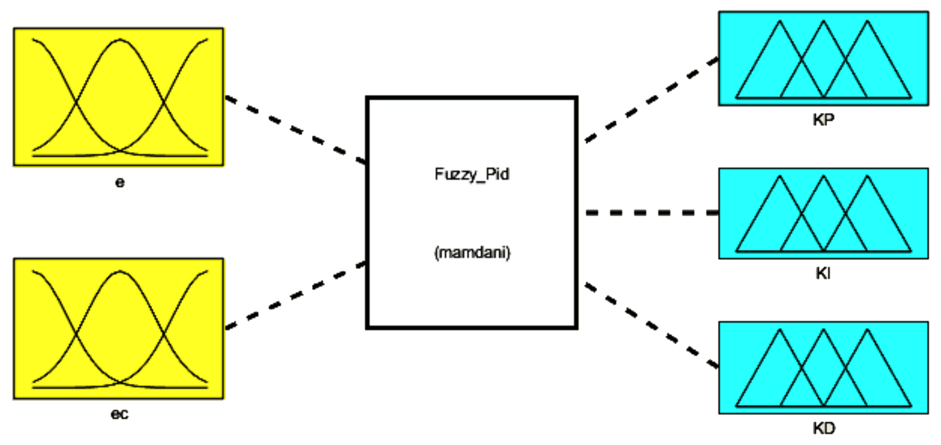
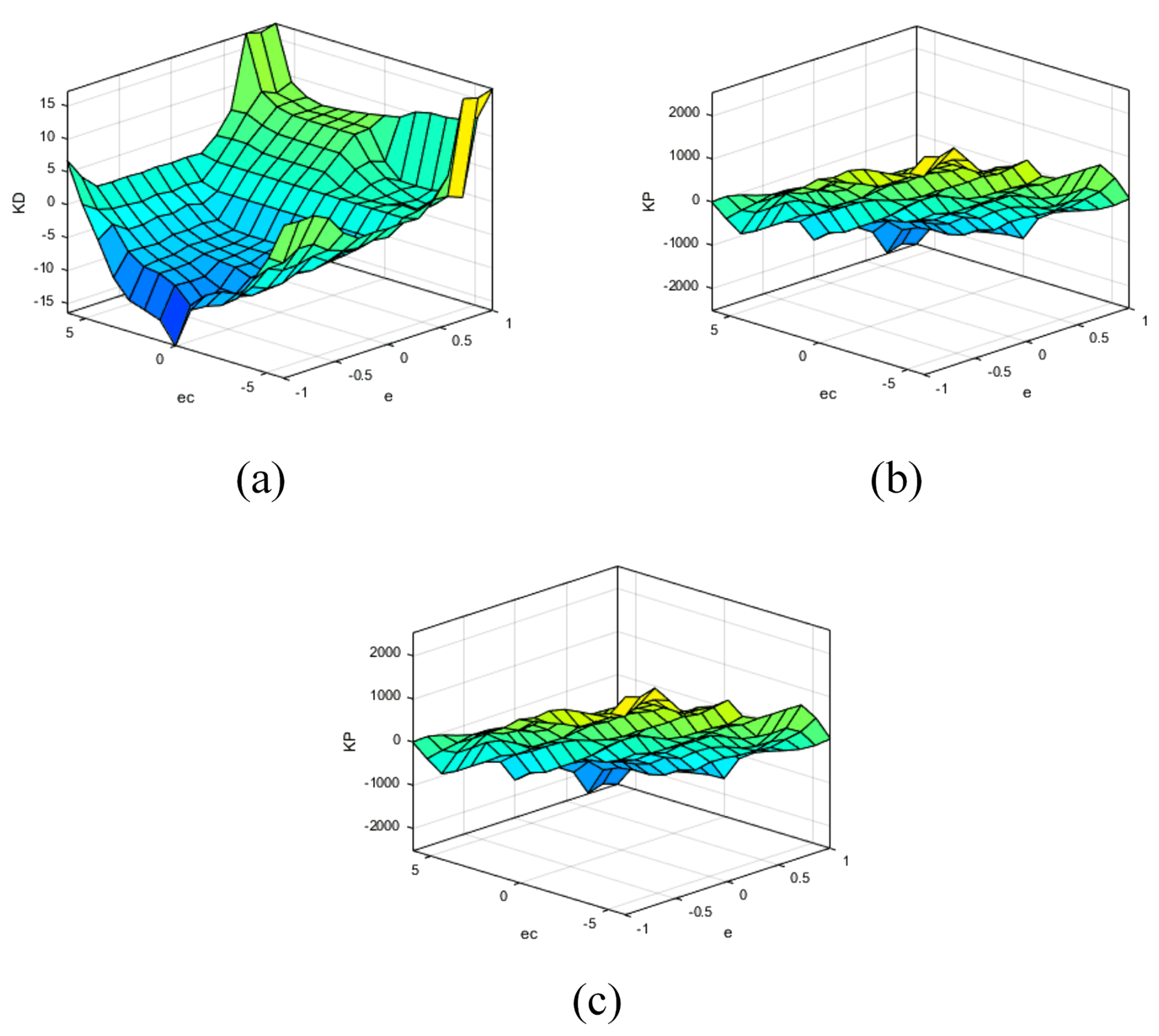
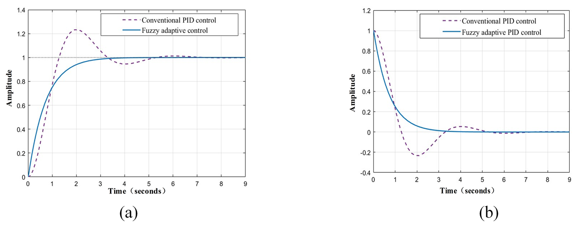
Figure 21 Step tracking and error analysis of fuzzy PID and PID: (a) step response comparison; (b) step tracking error comparison.

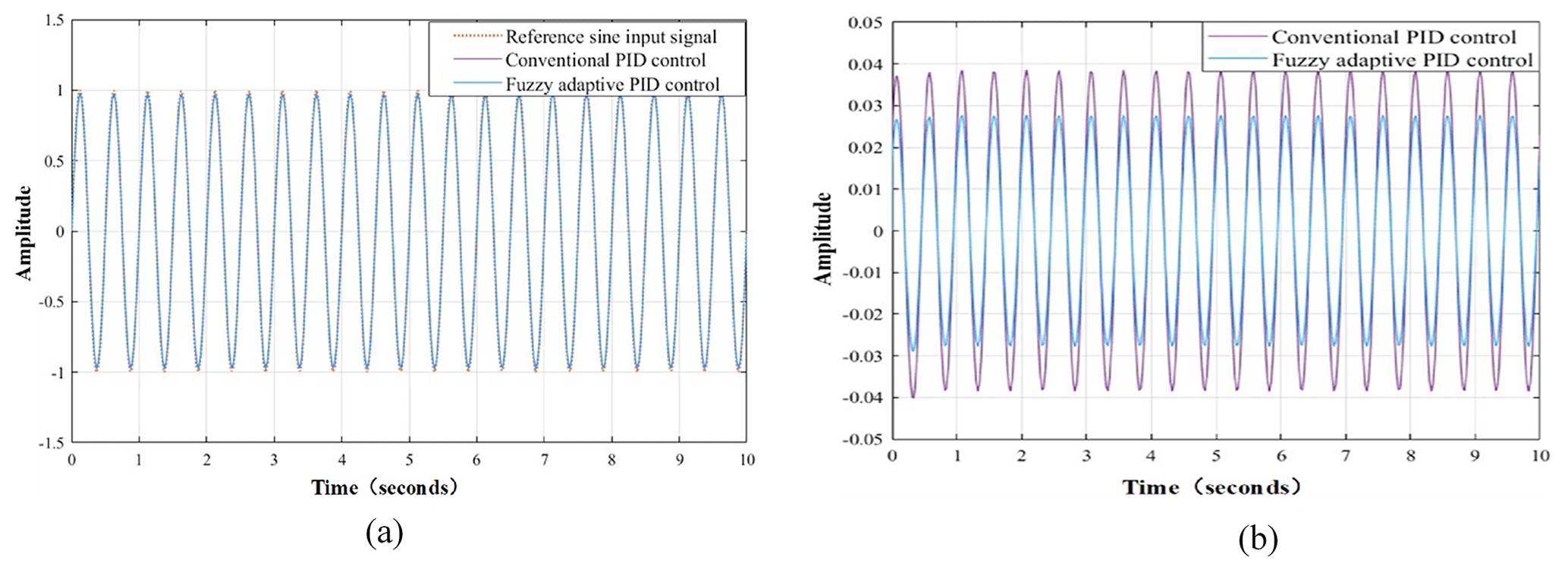
Figure 22 Sine tracking and error analysis of fuzzy PID and PID: (a) sine response comparison; (b) sine tracking error comparison.

The output variables K_p, K_i, and K_d of the fuzzy controller are solved by fuzzy inference and inverse fuzzification of the input variables e and ec. The fuzzy output value is taken as the output variable, K_p, K_i, or K_d, corresponding to the fuzzy value in its theoretical domain, and its scale factor is determined and multiplied with the output of the fuzzy controller to obtain the increment of the PID parameters K_p, K_i, and K_d. The control variables of the system are updated to produce a suppression effect on the system, and the corresponding adjustment algorithm is as follows:

$$\begin{array}{}\text{(39)}& \begin{array}{rl}& K_{\mathrm{p}}=K_{\mathrm{p}\mathrm{0}}+\mathrm{\Delta }{K}_{\mathrm{p}}\\ & K_{\mathrm{i}}=K_{\mathrm{i}\mathrm{0}}+\mathrm{\Delta }{K}_{\mathrm{i}}\\ & K_{\mathrm{d}}=K_{\mathrm{d}\mathrm{0}}+\mathrm{\Delta }{K}_{\mathrm{d}},\end{array}\end{array}$$

where K_p0, K_i0, and K_d0 are the initial values of K_p, K_i, and K_d , respectively.

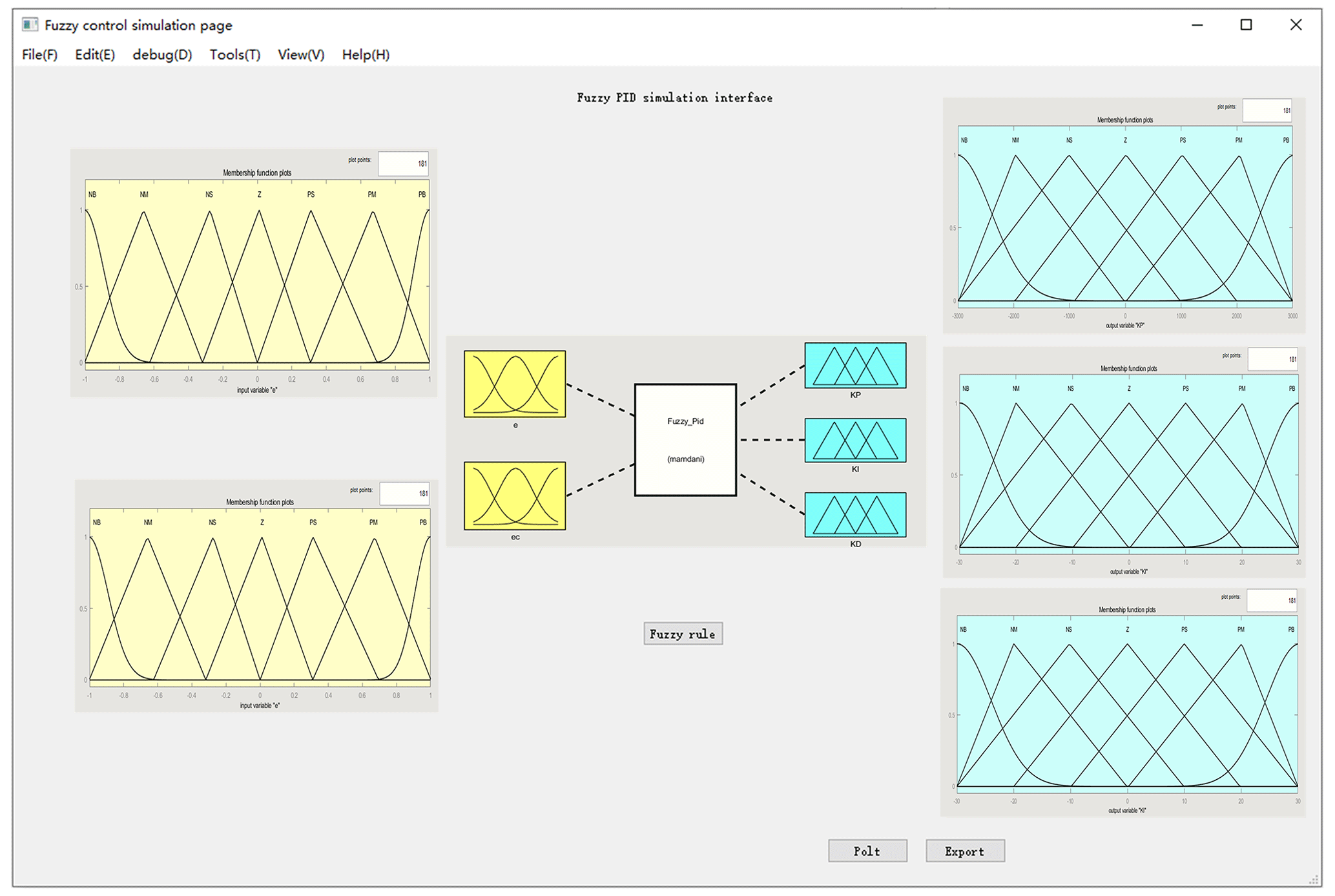
Figure 23 Fuzzy control interface diagram of MATLAB.

4.2.1 Simulation of fuzzy adaptive PID control system

The model diagram of the fuzzy adaptive PID control system is shown in Fig. 15.

On the base of fuzzy set theory, the input and output data should be transformed into proper variables with details as follows:

Input variables.

• system error e, domain of $[-\mathrm{1},\mathrm{1}]$, and scaling factor K_e=100;

• system error rate ec, domain of $[-\mathrm{6},\mathrm{6}]$ ° s⁻¹, and scaling factor K_c=100.

Output Variables.

• proportional gain increment ΔK_p, domain $[-\mathrm{3000},\mathrm{3000}]$, and scaling factor K₁=0.1;

• integral time increment K_i, domain $[-\mathrm{30},\mathrm{30}]$, and scaling factor K₂=0.1;

• derivative time increment ΔK_d, domain $[-\mathrm{20},\mathrm{20}]$, and scaling factor K₃=0.1.

This design enhances the sensitivity to dynamic disturbances through an expanded scaling factor while suppressing overshoot, thereby ensuring controller robustness under time-varying sea conditions. The input and output membership functions are shown in Figs. 16 and 17.

Once the affiliation functions of the two inputs and three outputs in the system are set, the control rules of the function will be edited as outlined in the following. The 49 rules are obtained through the fuzzy control table in the previous section. Figure 18 shows the fuzzy rule editing interface, and Fig. 19 shows the interface for defining the inputs and outputs.

From the fuzzy rules above, the surface relations of K_p, K_i, and K_d under fuzzy rules can be obtained in the setting of the fuzzy controller, as shown in Fig. 20.

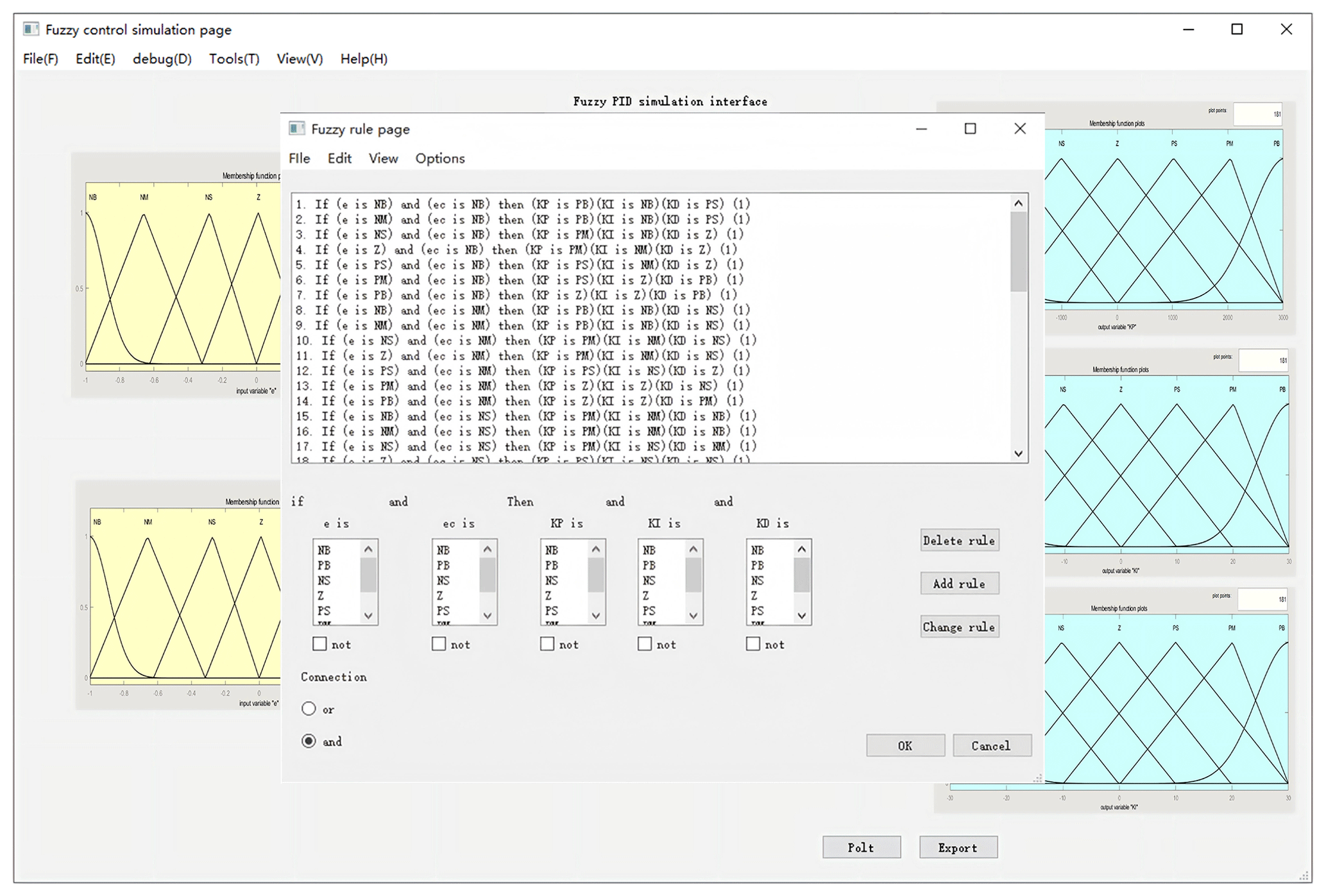
Figure 24 Input interface for the fuzzy control rules based on Qt Creator.

The control block diagram was established using Simulink, and the membership functions and rule base were input into the fuzzy controller. Figure 21 illustrates the step response and tracking error comparison between the fuzzy control system and the conventional PID control system, further revealing performance differences under varying signals.

Under a step input, the traditional PID exhibits a settling time of 7 s. Due to fixed parameter limitations, although the steady-state error approaches zero, significant overshoot (approximately 15 %) occurs during regulation (Fig. 21a), resulting in larger tracking errors in the transient phase (Fig. 21b). In contrast, the fuzzy adaptive PID dynamically adjusts parameters, reducing the settling time by 50 % and driving the tracking error close to zero without overshoot (Fig. 21b). This demonstrates the fuzzy PID's superior error suppression capability during dynamic phases, rapid stabilization, and enhanced control precision for step signals.

As shown in Fig. 22, the dashed line represents a sine signal with an amplitude of 1 and a frequency of 2 Hz, while the solid line denotes the actual output. The traditional PID, constrained by fixed parameters and limited bandwidth, accumulates high-frequency errors, leading to phase lag and steady-state error peaks in the tracking curve. The fuzzy PID, however, employs online parameter optimization to compensate for phase and amplitude deviations in real time. Its membership function design effectively suppresses periodic disturbances, resulting in near-perfect alignment between the tracking curve and the target signal. The steady-state error peak is controlled within 0.03°, with no amplitude attenuation, demonstrating robust performance and high real-time adaptability even under time-varying signals.

The fuzzy adaptive PID outperforms traditional PID in both step and sinusoidal signal scenarios, particularly under complex operating conditions (e.g., time-varying loads and nonlinear systems). While traditional PID relies on empirical parameter tuning, the fuzzy PID reduces manual intervention costs through its adaptive mechanism. Comparative analysis of tracking and error characteristics for step and sinusoidal signals confirms that the fuzzy adaptive PID significantly surpasses conventional PID with respect to settling time, overshoot suppression, steady-state accuracy, and phase compensation. Its multi-objective optimization capability provides an advanced solution for high-precision control systems.

4.3 User interface design for fuzzy control simulation of a shipboard stabilization platform

This interface is built mainly for the fuzzy control module; therefore, one can freely edit e and ec input and K_p, K_i, and K_d output in the interface. The main interface is shown in Fig. 23.

The user can click on the “Fuzzy rule” button to freely set the rules of fuzzy control. This rule interface greatly enhances input efficiency. The user can then click on the “OK” button to save the fuzzy control rules, as shown in Fig. 24.

According to the designed fuzzy control rules, the user can click on the “Plot” button, and the program will output the response curve of the set rules. The reference of the program itself comes with a PID control response curve.

5 Conclusions

A novel 6-DOF shipboard stabilization platform integrated with a fuzzy adaptive PID control was proposed to address the challenges involved with precision equipment operation in dynamic marine environments. The main contributions of this work are summarized as follows:

• To address the issues of limited workspace and low modeling accuracy in traditional ship stabilization platforms, a three-axis 6-DOF parallel mechanism was developed, which expands workspace and enables compensation for combined ship motions (roll, pitch, and yaw) through optimized hinge distribution with a workspace verified via Monte Carlo simulations. In addition, a dynamic modeling method for a non-inertial system based on the virtual-work principle is proposed, which solves the coupling error between the hull motion and the platform attitude.

• The proposed fuzzy adaptive PID controller achieved a 50 % reduction in settling time (7.0 to 3.5 s) and eliminated overshoot completely, with steady-state error constrained below 0.03° under 2 Hz sinusoidal excitation. The fuzzy system provided a scalable framework for marine control applications. The fuzzy adaptive PID controller demonstrates significant superiority over the conventional PID in terms of settling time reduction, overshoot suppression, steady-state accuracy, and phase compensation. Finally, a ship stabilization platform control user interface was designed based on Qt Creator and enabled real-time motion trajectory visualization and interactive fuzzy rule configuration.