Dynamic analysis and deploying process control of large parabolic cylinder antennas

The deployable parabolic cylindrical antenna, due to its large structural scale, complex transmission linkages, and multiple closed-loop constraints, endures significant differential loads on its structural components during the deployment process. This leads to substantial deformations or even damage to the structure. To enhance the reliability of the antenna's deployment and the load-bearing safety of its components, it is imperative to comprehensively identify the dynamic characteristics inherent in the control of the antenna deployment process. In this paper, a fast dynamic modeling method for large-scale, module-assembled, space deployable supporting structures is proposed. Based on this, an algorithm for solving high-dimensional differential equations which features polycondensation and recursion module by module is proposed. First, the dynamic and constraint equations are established for a large-scale deployable supporting structure with parabolic cylindrical surfaces which is divided into 25 sub-modules. Then, sub-modules are assembled to realize the fast dynamic modeling of the large-scale supporting structure. Further, an efficient recursive algorithm, which is solved module by module, is presented according to the concept of building dynamic equations in modularization. Finally, a nonlinear deployment control strategy based on velocity feedback is introduced to ensure stable deployment control over strongly nonlinear systems, such as the deployable supporting structure with parabolic cylindrical surfaces; moreover, ideal deployment control effects are achieved for such systems. The results indicate that the control method can reduce the peak velocity of the supporting structure during the deployment process from 5.508 to 0.0323 m s⁻¹ and that it improves the synchronicity of the antenna's supporting structure deployment by 69.49 %. This study provides a feasible implementation scheme for the dynamic characteristic analysis and deployable process control of back-shell truss antennas.

1 Introduction

The space antenna, which has been widely used in resource exploration, electronic reconnaissance, and deep space exploration, is the main component in space exploration missions (Liu et al., 2020; Chen et al., 2021; Lin et al., 2019). As a key core component of space antennas, deployable structures have achieved very rich research results of recent decades, such as solid-surface deployable structures, inflatable deployable mechanisms, and truss-type deployable structures, and the existing research work on deployable structures mainly focuses on deployable mechanism design. As the membrane deployable structure developed by Torisaka et al. (2019) and the cable–rib tension deployable antenna structure proposed by Liu et al. (2018), Sun et al. (2021) designed the H-style deployable mechanism for large space-borne mesh antennas. In order to improve the stiffness of the antenna, Han et al. (2019) designed a scissor double-ring truss deployable mechanism for space antennas. We also acknowledge the double-layer deployable truss structure designed by Dai and Xiao (2020) that meet the needs of large-diameter space antennas. Han et al. (2023) designed a new type of peripheral deployable antenna mechanism with an inner and outer height difference and verified the deployable degrees of freedom of this antenna based on screw theory. Shinde and Upadhyay (2024a) conducted in-depth research on membrane-type space deployable antennas, systematically investigating the effects of residual gas inflation under different folding patterns (Shinde and Upadhyay, 2024b) as well as the influence of tension on the surface shape, stress distribution, and overall stability of membrane reflectors (Shinde and Upadhyay, 2021, 2022, 2023). The parabolic cylindrical antenna studied in this paper is similar to other cable–rod deployable structures. It has the characteristics of large storage rate, light weight, and high precision. The parabolic antenna has become one of the new development directions of space-borne antennas (Hu et al., 2015).

The space deployable antenna is a typical rigid–flexible coupled multibody system. With the development of structural design, the diameter of the space-borne antenna is getting larger, and the influence of mechanism flexibility caused by the large-scale antenna deployment process is becoming more and more obvious (Hu et al., 2013). To improve the reliability of space antenna deployment and the safety of components under load, it is necessary to comprehensively identify the dynamic characteristics of antenna deployment using simulation and obtain the load characteristics of components during deployment. Therefore, scholars have carried out in-depth research on the dynamic characteristics of the antenna during deployment (Li, 2012; Fulton and Schaub, 2021; Lopatin et al., 2023). Establishing an accurate dynamic model of the large space deployable antenna is the basis of mechanical property analysis and deployment control.

ANCF (absolute nodal coordinate formulation) (Franco et al., 1998; Wang et al., 2022) is a well-known approach to solving the flexible multibody dynamics proposed by Jose Luis Escalona Franco and Ahmed A. Shabana in Franco et al. (1998), the dynamic equation has the characteristics of a constant inertia matrix, the absence of Coriolis force, and the centrifugal force, ANCF can describe the flexible multibody system more accurately and plays an important role in dealing with the dynamics of flexible multibody systems. Scholars have proposed a variety of ANCF units for cables, beams, plates, and shells (Ren and Fan, 2023; Otsuka et al., 2022; Wang and Sun, 2020), which are widely used in aerospace engineering (Cui et al., 2020; Feng et al., 2022). Li et al. (2016) studied the mesh finding analysis of peripheral loop truss antennas based on ANCF. You et al. (2021) used ANCF to establish the dynamics model of the F-DST (flower-like space deployable telescope) primary mirror for controlling the accuracy of the space telescope surface and attitude. Du et al. (2018) adopted the low-order beam element proposed by Gerstmayr and Shabana (2006) to discrete the flexible rods of the truss antenna structure, a cable element with a transition function is used to model the cable net from slack to tension state, and the deployment of antennas was analyzed. Peng et al. (2017) established a dynamic model of a large annular antenna based on geometrically accurate beams, and an optimization analysis was carried out on the deployment process to achieve smooth deployment. And the same, geometrically accurate beams were adopted by Ma et al. (2019) to study the mechanical behavior of flexible components during the deployment of large elliptical ring truss antennas. ANCF also has various aerospace applications, including assembling large modular satellite antennas (Li et al., 2019) and space deployable origami structures (Zhang et al., 2020; Wang et al., 2023). Although there are relatively in-depth studies on the influence of the flexible components (flexible trusses and large flexible cable nets) of the deployable support mechanism on the antenna deployment process (Zhang et al., 2017; Huang et al., 2020; Jin et al., 2021; Li et al., 2021). However, most of the existing research is focused on the field of peripheral deployable antennas. The research on large-scale parabolic cylindrical antennas with multiple closed loops and strong coupling characteristics is still shallow, and it is still in the configuration design stage. The parabolic cylindrical deployable antenna designed by Wang (2018) takes the plane eight-bar mechanism as the basic unit. The parabolic cylindrical antenna developed by Xiao et al. (2020) improves the stiffness by introducing a tension cable without significantly increasing the weight of the support mechanism. And Qin et al. (2020) designed a deployable parabolic cylindrical antenna by combining multiple scissor mechanism units. Unfortunately, there is little literature about the dynamic characteristics of this type of antenna during the deployment process. On the one hand, the parabolic cylindrical antenna has a complex structure, numerous supporting trusses, and complex types of motion pairs, which directly make it extremely difficult to establish its dynamic model. On the other hand, the existing kinds of literature on the dynamic behavior of large-scale deployable antennas often use the low-order beam element that is not subject to shear deformation and torsional deformation to reduce the amount of calculation (Campanelli et al., 2000), which makes it difficult to accurately simulate the dynamic behavior of the deployment process. If a dense three-dimensional full-parameter beam element is used to discretize the deployable truss, the scale of the dynamic equation of the final assembly is large, resulting in a time-consuming calculation. Moreover, an implicit integration algorithm is adopted to solve the high-dimensional differential-algebraic equations, which are needed to solve the elastic force Jacobian matrix at each iteration step, so it will further increase the difficulty of solving the dynamic equation and be time-consuming (Liu et al., 2010). Despite the availability of novel methods for lightweight and undamped deployable structures (Wang and Sun, 2020), as well as dimensionality reduction methods for dynamical differential equations (Peng et al., 2019), these approaches are not directly applicable to large and complex deployable parabolic cylindrical antennas.

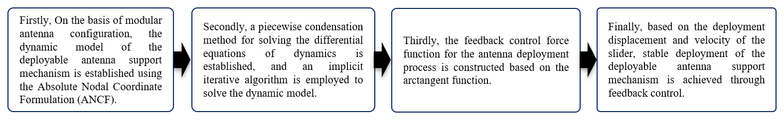
To analyze the dynamic characteristics of the deployment process of a large-scale shell deployable antenna with multi-closed-loop and strongly coupled features, the question of how to quickly establish an accurate dynamic model and use an efficient solution algorithm to obtain its dynamic characteristics remains to be further studied. The rest of this paper is as follows. The second part introduces the dynamic modeling method of the rigid–flexible coupled multibody system based on ANCF and NCF (natural coordinate formulation) methods. The third part obtains the dynamic model of the large-scale parabolic cylindrical deployable structure based on the idea of modular modeling. The fourth part proposes an efficient solution method of block-by-block condensation and recursion based on the research content of the third part. In the fifth part, the dynamic characteristics of the parabolic cylindrical deployable structure are studied, and a nonlinear deployment control method based on velocity feedback is proposed to ensure the stability of the deployable structure during the deployable process. In the final section, conclusions are drawn. The research procedure of this paper is illustrated in Fig. 1.

Figure 1 Research procedure of this paper.

2 Dynamic model of the parabolic cylindrical deployable structure

2.1 Rigid beam element based on NCF

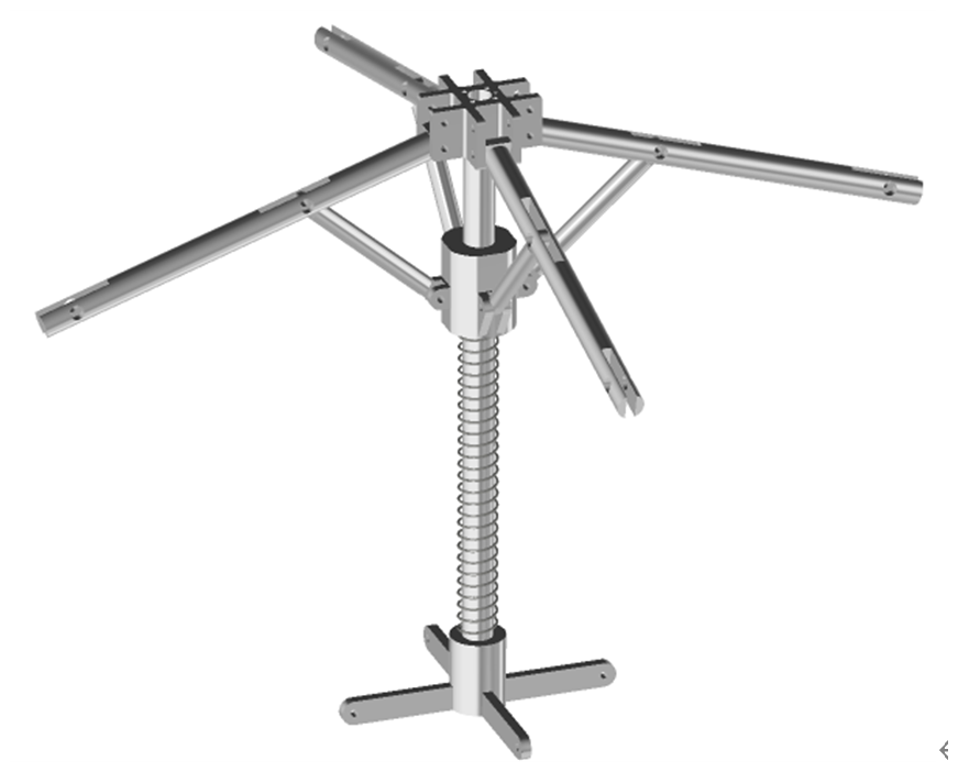
The parabolic cylindrical deployable structure is driven by the elastic potential energy stored in the drive component (Fig. 2). During the expansion process, the elastic deformation of the drive component can be ignored; therefore, each connector in the drive component is regarded as a rigid body, and the NCF element (de Jalón, 2007) that can obtain the constant mass matrix can be adopted, as shown in Fig. 3.

Figure 2 Drive component.

Figure 3 NCF element.

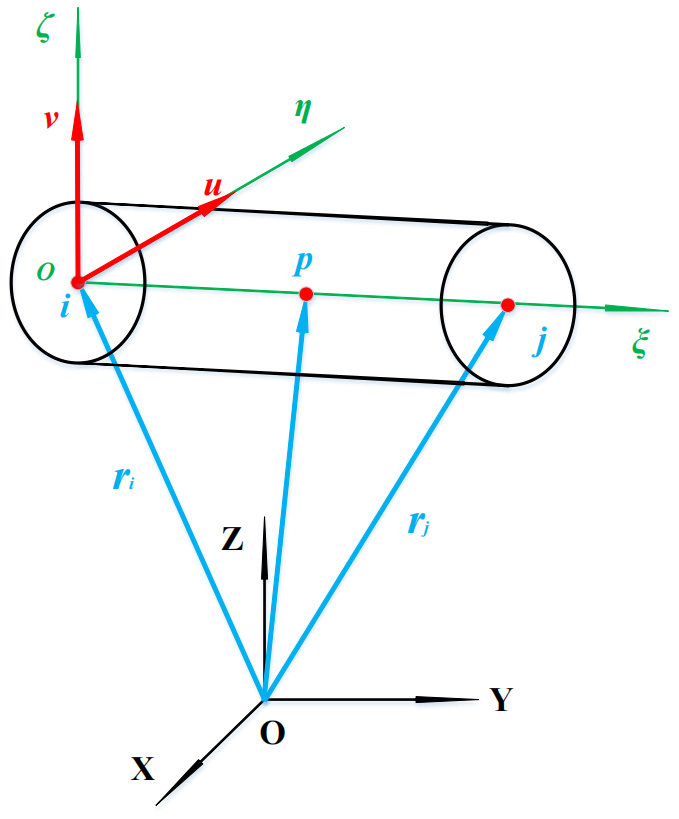
The NCF element adopts the position coordinates [r_i,r_j] of the two endpoints on the space rigid body in the global coordinate system, and the coordinates [u,v] of the two perpendicular coplanar unit vectors are used as the generalized coordinates q_e; that is, the following applies:

$$\begin{array}{}\text{(1)}& {\mathbf{q}}_e={\left[\begin{array}{cccc}{\mathit{r}}_i^{\mathrm{T}}& {\mathit{r}}_j^{\mathrm{T}}& {\mathit{u}}^{\mathrm{T}}& {\mathit{v}}^{\mathrm{T}}\end{array}\right]}^{\mathrm{T}}.\end{array}$$

Construct the local coordinate system O_ξηζ of the NCF rigid beam element using the vectors $({\mathit{r}}_i,{\mathit{r}}_j,\mathit{u},\mathit{v})$ so the position coordinates of any point p on the rigid body in the local coordinate system can be represented as $[L{c}_{\mathrm{1}},c_{\mathrm{2}},c_{\mathrm{3}}]$, where L is the length of the rigid beam; then, the coordinate array of point p in the global coordinate system can be expressed as Eq. (2):

$$\begin{array}{}\text{(2)}& \begin{array}{rl}{\mathit{r}}_p& ={\mathit{r}}_i+c_{\mathrm{1}}\left({\mathit{r}}_j-{\mathit{r}}_i\right)+c_{\mathrm{2}}\mathit{u}+c_{\mathrm{3}}\mathit{v}\\ & =\left[\begin{array}{cccc}(\mathrm{1}-c_{\mathrm{1}})\mathbf{I}& c_{\mathrm{1}}\mathbf{I}& c_{\mathrm{2}}\mathbf{I}& c_{\mathrm{3}}\mathbf{I}\end{array}\right]\left[\begin{array}{c}{\mathit{r}}_i\\ {\mathit{r}}_j\\ \mathit{u}\\ \mathit{v}\end{array}\right]\\ & ={\mathbf{C}}_p{\mathbf{q}}_e.\end{array}\end{array}$$

Here, ${\mathbf{C}}_p\in {\mathbb{R}}^{\mathrm{3}\times \mathrm{12}}$, $\mathbf{I}\in {\mathbb{R}}^{\mathrm{3}\times \mathrm{3}}$, and I is the identity matrix. Since c₁, c₂, and c₃ are constant, the matrix C_p is also constant. The NCF element has 12 generalized coordinates, while the rigid body in space has only 6 degrees of freedom. Therefore, there are the following six constraints between r_i, r_j, u, and v:

$$\begin{array}{}\text{(3)}& \left\{\begin{array}{l}∥{\mathit{r}}_j-{\mathit{r}}_i∥=L,∥\mathit{u}∥=\mathrm{1},∥\mathit{v}∥=\mathrm{1},\\ \left({\mathit{r}}_j-{\mathit{r}}_i\right)\perp \mathit{u},\left({\mathit{r}}_j-{\mathit{r}}_i\right)\perp \mathit{v},\mathit{u}\perp \mathit{v}\end{array}\right..\end{array}$$

2.2 Flexible full parameter beam element based on ANCF

Because of the complex connection form of the parabolic cylindrical antenna, there is a component force along the arc direction leading to the connecting unit in the deployable structure having to bear the shear force and torsion force. If the low-order beam element of ANCF is used, it is difficult to accurately simulate the influence of torsion and shear during the deployment process of the flexible beam in the parabolic cylindrical deployable structure. Therefore, this paper adopts the full-parameter beam element of ANCF which can accurately simulate the mechanical characteristics of flexible components.

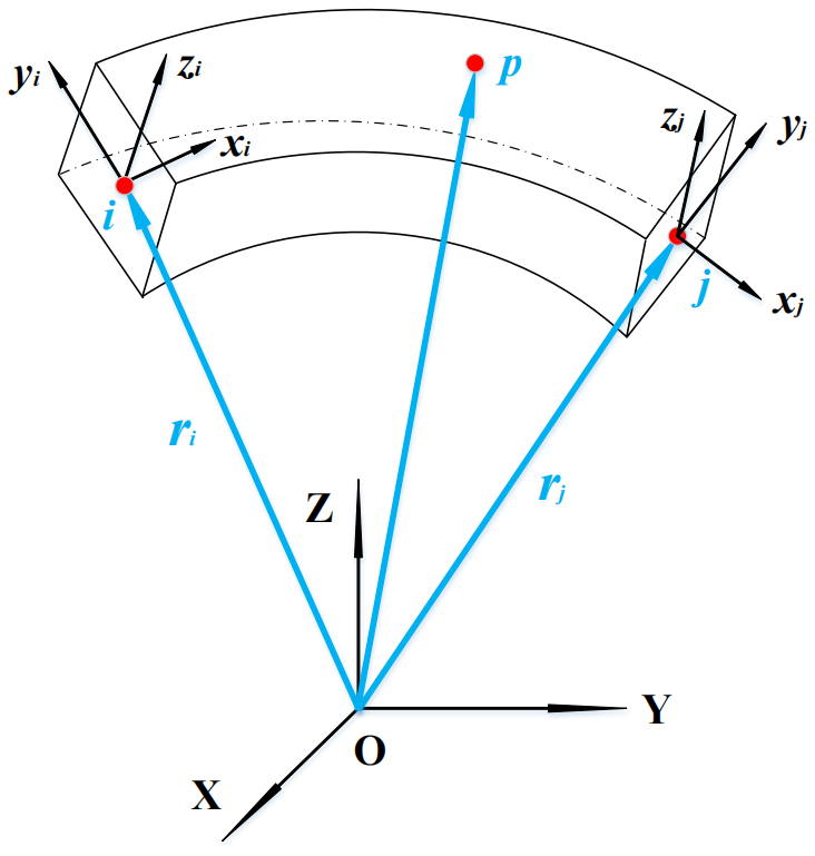
Compared with the low-order beam element, the full-parametric beam (Fig. 4) introduces the displacement gradient within the beam section, so the beam endpoint e_i contains 12 nodal coordinates:

$$\begin{array}{}\text{(4)}& {\mathbf{e}}_i^{\mathrm{T}}={\left[\begin{array}{cccc}{\mathit{r}}^{\mathrm{T}}& {\mathit{r}}_x^{\mathrm{T}}& {\mathit{r}}_y^{\mathrm{T}}& {\mathit{r}}_z^{\mathrm{T}}\end{array}\right]}^{\mathrm{T}}.\end{array}$$

The vector r^T is used to describe the position coordinates of the node i in the global coordinate system, and $\left[\begin{array}{ccc}{\mathit{r}}_x^{\mathrm{T}}& {\mathit{r}}_y^{\mathrm{T}}& {\mathit{r}}_z^{\mathrm{T}}\end{array}\right]$ is the position vector gradient; derivatives of the position vector concerning coordinates x, y, and z are

$$\begin{array}{}\text{(5)}& \mathit{r}={\left[\begin{array}{ccc}{X}_i& Y_i& Z_i\end{array}\right]}^{\mathrm{T}},{\mathit{r}}_x={\displaystyle \frac{\partial \mathit{r}}{\partial x}},{\mathit{r}}_y={\displaystyle \frac{\partial \mathit{r}}{\partial y}},{\mathit{r}}_z={\displaystyle \frac{\partial \mathit{r}}{\partial z}}.\end{array}$$

According to the continuity of the element, the global position coordinate r of any point p in the beam element is the interpolation function of the coordinates of the end node of the beam, which can be expressed by the shape function

$$\begin{array}{}\text{(6)}& \begin{array}{rl}{\mathit{r}}_p& =\mathbf{S}(x,y,z)\mathbf{e}\\ & =\left[\begin{array}{cccccccc}{S}_{\mathrm{1}}\mathbf{I}& S_{\mathrm{2}}\mathbf{I}& S_{\mathrm{3}}\mathbf{I}& S_{\mathrm{4}}\mathbf{I}& S_{\mathrm{5}}\mathbf{I}& S_{\mathrm{6}}\mathbf{I}& S_{\mathrm{7}}\mathbf{I}& S_{\mathrm{8}}\mathbf{I}\end{array}\right]\mathbf{e}\end{array},\end{array}$$

where $\mathbf{I}\in {\mathbb{R}}^{\mathrm{3}\times \mathrm{3}}$ is the identity matrix and the specific form of the shape function is as follows:

$$\begin{array}{}\text{(7)}& \begin{array}{rl}& \left\{\begin{array}{ll}{S}_{\mathrm{1}}=\mathrm{1}-\mathrm{3}{\mathit{\xi }}^{\mathrm{2}}+\mathrm{2}{\mathit{\xi }}^{\mathrm{3}}& S_{\mathrm{2}}=L(\mathit{\xi }-\mathrm{2}{\mathit{\xi }}^{\mathrm{2}}+{\mathit{\xi }}^{\mathrm{3}})\\ S_{\mathrm{3}}=L(\mathit{\eta }-\mathit{\xi }\mathit{\eta })& S_{\mathrm{4}}=L(\mathit{\zeta }-\mathit{\xi }\mathit{\zeta })\\ S_{\mathrm{5}}=\mathrm{3}{\mathit{\xi }}^{\mathrm{2}}-\mathrm{2}{\mathit{\xi }}^{\mathrm{3}}& S_{\mathrm{6}}=L(-{\mathit{\xi }}^{\mathrm{2}}+{\mathit{\xi }}^{\mathrm{3}})\\ S_{\mathrm{7}}=L\mathit{\xi }\mathit{\eta }& S_{\mathrm{8}}=L\mathit{\xi }\mathit{\zeta }\end{array}\right.,\\ & \mathbf{e}=[\begin{array}{cc}{\mathbf{e}}_i^{\mathrm{T}}& {\mathbf{e}}_j^{\mathrm{T}}\end{array}{]}^{\mathrm{T}}\\ & ={\left[\begin{array}{cccccccc}{\mathit{r}}_i^{\mathrm{T}}& {\mathit{r}}_{ix}^{\mathrm{T}}& {\mathit{r}}_{iy}^{\mathrm{T}}& {\mathit{r}}_{iz}^{\mathrm{T}}& {\mathit{r}}_j^{\mathrm{T}}& {\mathit{r}}_{jx}^{\mathrm{T}}& {\mathit{r}}_{jy}^{\mathrm{T}}& {\mathit{r}}_{jz}^{\mathrm{T}}\end{array}\right]}^{\mathrm{T}}.\end{array}\end{array}$$

Here, r_ix, r_iy, and r_iz denote the position gradient vectors along the x, y, and z directions in the local coordinate system for node i. L represents the length of the beam element. According to the continuum mechanics theory, the deformation gradient tensor G is used to represent the changing relationship between the initial configuration r₀ of the elastic body and the current configuration r after the movement, and the local coordinate system fixed on the material is denoted as $\mathit{\alpha }(\mathit{\alpha }=x,y,z)$.

$$\begin{array}{}\text{(8)}& \mathbf{G}={\displaystyle \frac{\partial \mathit{r}}{\partial {\mathit{r}}_{\mathrm{0}}}}={\displaystyle \frac{\partial \mathit{r}}{\partial \mathit{\alpha }}}{\displaystyle \frac{\partial \mathit{\alpha }}{\partial {\mathit{r}}_{\mathrm{0}}}}\end{array}$$

To facilitate the solution of the elastic force and force Jacobian of the element, the position vector r_p, can be rewritten as

$$\begin{array}{}\text{(9)}& {\mathit{r}}_p=\stackrel{\mathrm{‾}}{\mathbf{e}}\stackrel{\mathrm{‾}}{\mathbf{S}},\end{array}$$

where $\stackrel{\mathrm{‾}}{\mathbf{S}}\in {\mathbb{R}}^{\mathrm{8}\times \mathrm{1}},\stackrel{\mathrm{‾}}{\mathbf{e}}\in {\mathbb{R}}^{\mathrm{3}\times \mathrm{8}}$, and the specific form is as follows:

$$\begin{array}{}\text{(10)}& \left\{\begin{array}{l}\stackrel{\mathrm{‾}}{\mathbf{S}}=[\begin{array}{cccccccc}{S}_{\mathrm{1}}& S_{\mathrm{2}}& S_{\mathrm{3}}& S_{\mathrm{4}}& S_{\mathrm{5}}& S_{\mathrm{6}}& S_{\mathrm{7}}& S_{\mathrm{8}}\end{array}{]}^{\mathrm{T}}\\ \stackrel{\mathrm{‾}}{\mathbf{e}}=\left[\begin{array}{cccccccc}{e}_{\mathrm{1}}& e_{\mathrm{4}}& e_{\mathrm{7}}& e_{\mathrm{10}}& e_{\mathrm{13}}& e_{\mathrm{16}}& e_{\mathrm{19}}& e_{\mathrm{22}}\\ e_{\mathrm{2}}& e_{\mathrm{5}}& e_{\mathrm{8}}& e_{\mathrm{11}}& e_{\mathrm{14}}& e_{\mathrm{17}}& e_{\mathrm{20}}& e_{\mathrm{23}}\\ e_{\mathrm{3}}& e_{\mathrm{6}}& e_{\mathrm{9}}& e_{\mathrm{12}}& e_{\mathrm{15}}& e_{\mathrm{18}}& e_{\mathrm{21}}& e_{\mathrm{24}}\end{array}\right]\end{array}\right..\end{array}$$

Therefore, the position gradient is written as follows:

$$\begin{array}{}\text{(11)}& \mathbf{G}=\stackrel{\mathrm{‾}}{\mathbf{e}}{\displaystyle \frac{\partial \stackrel{\mathrm{‾}}{\mathbf{S}}}{\partial \mathit{\alpha }}}{\left({\displaystyle \frac{\partial {\mathit{r}}_{\mathrm{0}}}{\partial \mathit{\alpha }}}\right)}^{-\mathrm{1}}=\stackrel{\mathrm{‾}}{\mathbf{e}H}.\end{array}$$

The following also applies:

$$\begin{array}{}\text{(12)}& \mathbf{H}={\displaystyle \frac{\partial \stackrel{\mathrm{‾}}{\mathbf{S}}}{\partial \mathit{\alpha }}}{\left({\displaystyle \frac{\partial {\mathit{r}}_{\mathrm{0}}}{\partial \mathit{\alpha }}}\right)}^{-\mathrm{1}}.\end{array}$$

H contains the reference configuration information of the beam element. According to the expression, H is a time-independent matrix, and the elastic force virtual work can be expressed as follows (Gerstmayr and Shabana, 2005):

$$\begin{array}{}\text{(13)}& \mathit{\delta }U=\int \mathit{E}:\mathit{\delta }\mathit{\epsilon }\mathrm{d}V=\int \mathit{P}:\mathit{\delta }\mathbf{G}\mathrm{d}V.\end{array}$$

Here, E is the second Piola–Kirchhoff stress tensor, ε is the Green strain tensor, P is the first Piola–Kirchhoff stress tensor, and the elastic force of element can be expressed by the differential of strain energy to generalized coordinates:

$$\begin{array}{}\text{(14)}& {\mathbf{Q}}^e=-{\displaystyle \frac{\partial U}{\partial e}}=-\int \mathit{P}:{\displaystyle \frac{\partial G}{\partial e}}\mathrm{d}V.\end{array}$$

The component of the elastic force is

$$\begin{array}{}\text{(15)}& Q_i^e=-\int {\mathit{P}}_{\mathrm{kl}}{\displaystyle \frac{\partial G_{\mathrm{kl}}}{\partial e_i}}\mathrm{d}V.\end{array}$$

We introduce the following:

$$\begin{array}{}\text{(16)}& e_i={\stackrel{\mathrm{‾}}{e}}_{\mathrm{rs}},i=\mathrm{3}(s-\mathrm{1})+r,(s=\mathrm{1},\mathrm{2},\mathrm{\dots },\mathrm{8},r=\mathrm{1},\mathrm{2},\mathrm{3}).\end{array}$$

Therefore, Eq. (15) can be expressed as

$$\begin{array}{}\text{(17)}& \begin{array}{rl}{Q}_i^e& =-\int {\mathit{P}}_{\mathrm{kl}}{\displaystyle \frac{\partial G_{\mathrm{kl}}}{\partial {\stackrel{\mathrm{‾}}{e}}_{\mathrm{rs}}}}\mathrm{d}V=-\int {\mathit{P}}_{\mathrm{kl}}{\displaystyle \frac{\partial \left({\stackrel{\mathrm{‾}}{e}}_{\mathrm{km}}{H}_{\mathrm{ml}}\right)}{\partial {\stackrel{\mathrm{‾}}{e}}_{\mathrm{rs}}}}\mathrm{d}V\\ & =-\int {\mathit{P}}_{\mathrm{kl}}{\mathit{\delta }}_{\mathrm{kr}}{\mathit{\delta }}_{\mathrm{ms}}{H}_{\mathrm{ml}}\mathrm{d}V\\ & =-\int {\mathit{P}}_{\mathrm{rl}}{H}_{\mathrm{sl}}\mathrm{d}V,\end{array}\end{array}$$

where δ_kr and δ_ms are Kronecker δ and P can be represented by G and E.

$$\begin{array}{}\text{(18)}& P_{\mathrm{rl}}=G_{\mathrm{rn}}{E}_{\mathrm{nl}}=\left({\stackrel{\mathrm{‾}}{e}}_{\mathrm{rt}}{H}_{\mathrm{tn}}\right)\left[{\displaystyle \frac{\mathrm{1}}{\mathrm{2}}}{D}_{\mathrm{nlab}}\left(G_{\mathrm{ac}}^{\mathrm{T}}{G}_{\mathrm{cb}}-{\mathrm{\Im }}_{\mathrm{ab}}\right)\right]\end{array}$$

Here, D_nlab represents the component of the fourth-order elastic tensor, ℑ_ab represents the component of the second-order unit tensor:

$$\begin{array}{}\text{(19)}& \left\{\begin{array}{l}\begin{array}{rl}{D}_{\mathrm{nlab}}& =\mathit{\lambda }{\mathit{\delta }}_{\mathrm{nl}}{\mathit{\delta }}_{\mathrm{ab}}{\mathbf{g}}_n\otimes {\mathbf{g}}_l\otimes {\mathbf{g}}_a\otimes {\mathbf{g}}_b\\ & +\mathrm{2}\mathit{\mu }{\mathit{\delta }}_{\mathrm{na}}{\mathit{\delta }}_{\mathrm{lb}}{\mathbf{g}}_n\otimes {\mathbf{g}}_a\otimes {\mathbf{g}}_l\otimes {\mathbf{g}}_b\end{array}\\ \mathrm{\Im }={\mathit{\delta }}_{\mathrm{ab}}{\mathbf{g}}_a\otimes {\mathbf{g}}_b\end{array}\right.,\end{array}$$

where g_a, g_b, g_n, and g_l are the basis vectors and λ and μ are the Lamé constants; then, we can substitute the component of P into the elastic force.

$$\begin{array}{}\text{(20)}& \begin{array}{rl}{Q}_i^e& =-\int \left({\stackrel{\mathrm{‾}}{e}}_{\mathrm{rt}}{H}_{\mathrm{tn}}\right)\left[{\displaystyle \frac{\mathrm{1}}{\mathrm{2}}}{D}_{\mathrm{nlab}}\left(G_{\mathrm{ac}}^{\mathrm{T}}{G}_{\mathrm{cb}}-{\mathrm{\Im }}_{\mathrm{ab}}\right)\right]H_{\mathrm{sl}}\mathrm{d}V\\ & =-{\displaystyle \frac{\mathrm{1}}{\mathrm{2}}}\int D_{\mathrm{nlab}}\left({\stackrel{\mathrm{‾}}{e}}_{\mathrm{rt}}{H}_{\mathrm{tn}}\right)\left({\stackrel{\mathrm{‾}}{e}}_{\mathrm{cf}}{H}_{\mathrm{fa}}{\stackrel{\mathrm{‾}}{e}}_{\mathrm{cv}}{H}_{\mathrm{vb}}-{\mathrm{\Im }}_{\mathrm{ab}}\right)H_{\mathrm{sl}}\mathrm{d}V\\ & =-{\displaystyle \frac{\mathrm{1}}{\mathrm{2}}}\int D_{\mathrm{nlab}}{H}_{\mathrm{fa}}{H}_{\mathrm{vb}}{H}_{\mathrm{tn}}{H}_{\mathrm{sl}}\mathrm{d}V{\stackrel{\mathrm{‾}}{e}}_{\mathrm{rt}}{\stackrel{\mathrm{‾}}{e}}_{\mathrm{cf}}{\stackrel{\mathrm{‾}}{e}}_{\mathrm{cv}}\\ & +{\displaystyle \frac{\mathrm{1}}{\mathrm{2}}}\int D_{\mathrm{nlab}}{\mathrm{\Im }}_{\mathrm{ab}}{H}_{\mathrm{tn}}{H}_{\mathrm{sl}}\mathrm{d}V{\stackrel{\mathrm{‾}}{e}}_{\mathrm{rt}}\\ & ={\displaystyle \frac{\mathrm{1}}{\mathrm{2}}}{K}_{\mathrm{ts}}^{\mathrm{I}}{\stackrel{\mathrm{‾}}{e}}_{\mathrm{rt}}-{\displaystyle \frac{\mathrm{1}}{\mathrm{2}}}{K}_{\mathrm{fvts}}^{\mathrm{II}}{\stackrel{\mathrm{‾}}{e}}_{\mathrm{rt}}{\stackrel{\mathrm{‾}}{e}}_{\mathrm{cf}}{\stackrel{\mathrm{‾}}{e}}_{\mathrm{cv}}\end{array}\end{array}$$

H is a time-independent matrix as indicated above, so $K_{\mathrm{ts}}^{\mathrm{I}}$ and $K_{\mathrm{fvts}}^{\mathrm{II}}$ are constant stiffness matrices that can be stored in the computer during the pre-processing. Liu et al. (2010) further derived the Jacobian analytic formula for elastic force based on Gerstmayr's work.

$$\begin{array}{}\text{(21)}& J_{ij}={\displaystyle \frac{\partial Q_i^e}{\partial e_j}}\end{array}$$

We introduce the following:

$$\begin{array}{}\text{(22)}& e_j={\stackrel{\mathrm{‾}}{e}}_{\mathit{\alpha }\mathit{\beta }},j=\mathrm{3}(\mathit{\beta }-\mathrm{1})+\mathit{\alpha },(\mathit{\beta }=\mathrm{1},\mathrm{2},\mathrm{\dots },\mathrm{8},\mathit{\alpha }=\mathrm{1},\mathrm{2},\mathrm{3}).\end{array}$$

The analytic formula is

$$\begin{array}{}\text{(23)}& \begin{array}{rl}{J}_{ij}& ={\displaystyle \frac{\partial \left(\frac{\mathrm{1}}{\mathrm{2}}{K}_{\mathrm{ts}}^{\mathrm{I}}{\stackrel{\mathrm{‾}}{e}}_{\mathrm{rt}}-\frac{\mathrm{1}}{\mathrm{2}}{K}_{\mathrm{fvts}}^{\mathrm{II}}{\stackrel{\mathrm{‾}}{e}}_{\mathrm{rt}}{\stackrel{\mathrm{‾}}{e}}_{\mathrm{cf}}{\stackrel{\mathrm{‾}}{e}}_{\mathrm{cv}}\right)}{\partial {\stackrel{\mathrm{‾}}{e}}_{\mathit{\alpha }\mathit{\beta }}}}\\ & ={\displaystyle \frac{\mathrm{1}}{\mathrm{2}}}{K}_{\mathrm{ts}}^{\mathrm{I}}{\mathit{\delta }}_{r\mathit{\alpha }}{\mathit{\delta }}_{t\mathit{\beta }}-{\displaystyle \frac{\mathrm{1}}{\mathrm{2}}}{K}_{\mathrm{fvts}}^{\mathrm{II}}{\mathit{\delta }}_{r\mathit{\alpha }}{\mathit{\delta }}_{t\mathit{\beta }}{\stackrel{\mathrm{‾}}{e}}_{\mathrm{cf}}{\stackrel{\mathrm{‾}}{e}}_{\mathrm{cv}}\\ & -{\displaystyle \frac{\mathrm{1}}{\mathrm{2}}}{K}_{\mathrm{fvts}}^{\mathrm{II}}{\stackrel{\mathrm{‾}}{e}}_{\mathrm{rt}}\left({\mathit{\delta }}_{c\mathit{\alpha }}{\mathit{\delta }}_{f\mathit{\beta }}{\stackrel{\mathrm{‾}}{e}}_{\mathrm{cv}}+{\mathit{\delta }}_{c\mathit{\alpha }}{\mathit{\delta }}_{v\mathit{\beta }}{\stackrel{\mathrm{‾}}{e}}_{\mathrm{cf}}\right)\end{array}.\end{array}$$

Figure 4 ANCF full-parameter beam elements.

2.3 Dynamic modeling based on ANCF-NCF method

The parabolic cylindrical deployable structure studied in this paper is shown in Fig. 5; the deployable truss is composed of two basic sub-rings, a basic unit on the directrix (BUD) and a main basic unit on the generatrix (MBUG). C₀ is the connection point between the deployable structure and the satellite manipulator, which is the boundary constraint.

Figure 5 Parabolic cylindrical deployable structure.

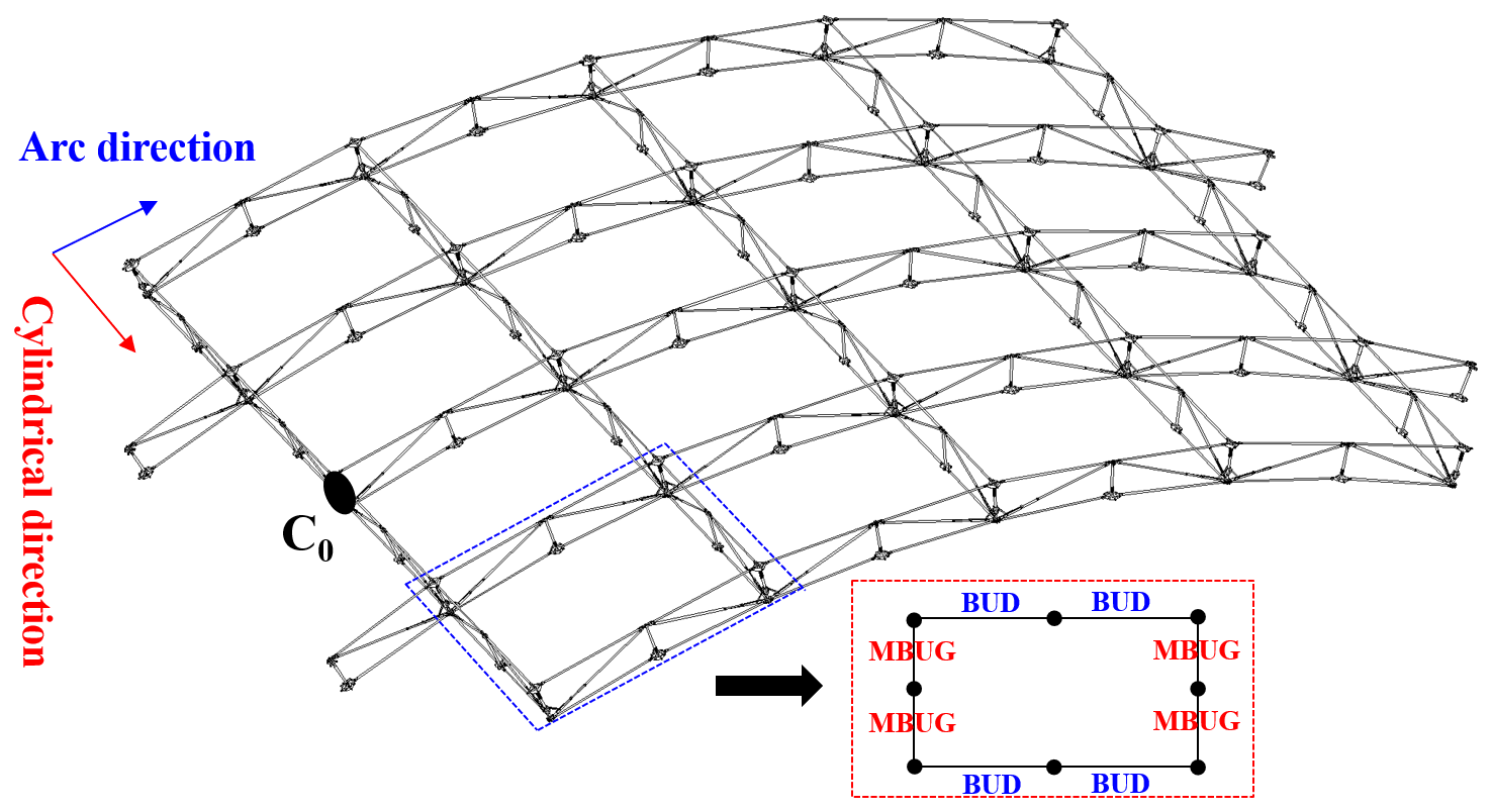
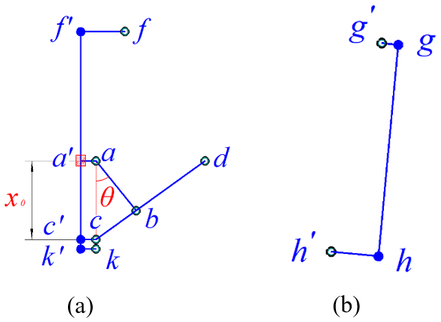
The BUD and MBUG basic sub-rings have the same geometric configuration (Fig. 6) but different sizes. The deployable units are all driven by the cylindrical spring to push the slider a to move in the negative direction of the Y axis and then drive each link moving to make the basic sub-ring gradually expand until the connecting rod (de) touches the mechanical limit point H, the machine stops moving, and the basic sub-ring is in a self-locking state. The intersecting basic sub-rings are driven by the same slider, as shown in Fig. 8.

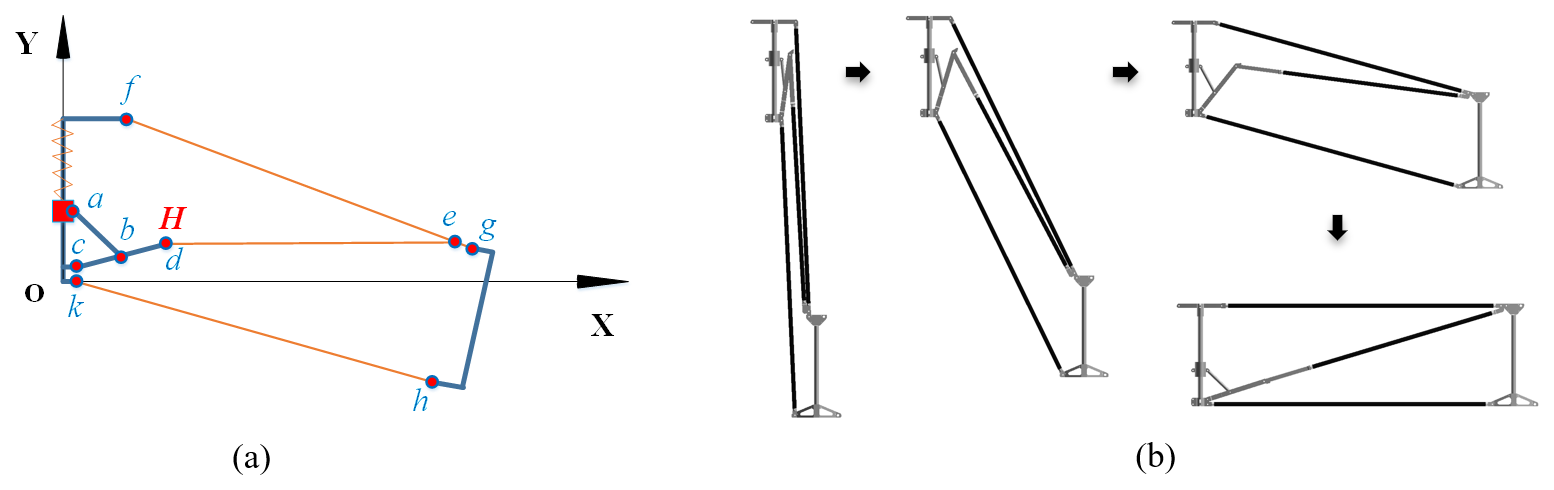
Figure 6 Configuration of BUD and MBUG. (a) Configuration. (b) Folding and deployment configuration of BUD and MBUG.

The dynamic model of the parabolic cylindrical structure is extremely complicated, which is embodied by establishing the constraint equation between large-scale generalized coordinates and setting up the Jacobian matrix of the constraint equation. The deployable antenna studied in this paper is a rigid–flexible coupled multibody system with many hinge constraints, sliding constraints, and rigid constraints. It is undoubtedly a great challenge to establish the constraint equations of the system one by one. Fortunately, the overall configuration of such a large back-shell antenna system can be split into several sub-modules. Therefore, the parabolic cylindrical antenna studied in this paper can be divided into 25 sub-modules as shown in Fig. 7.

Figure 7 Assembly configuration.

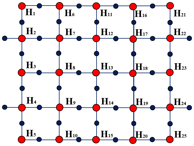
The 25 sub-modules in Fig. 7 are all composed of BUD and MBUG sub-rings. According to the splicing method of sub-rings in each sub-module, it can be classified into nine basic modules (I₀–I₈) in Table 1. Through further analysis of the geometric assembly configuration of I₀–I₈ modules, eight basic modules (I₁–I₈) can be directly obtained by cutting and removing partial molecular rings of the basic module I₀ (Fig. 8).

Table 1 Mapping between basic module and sub-module.

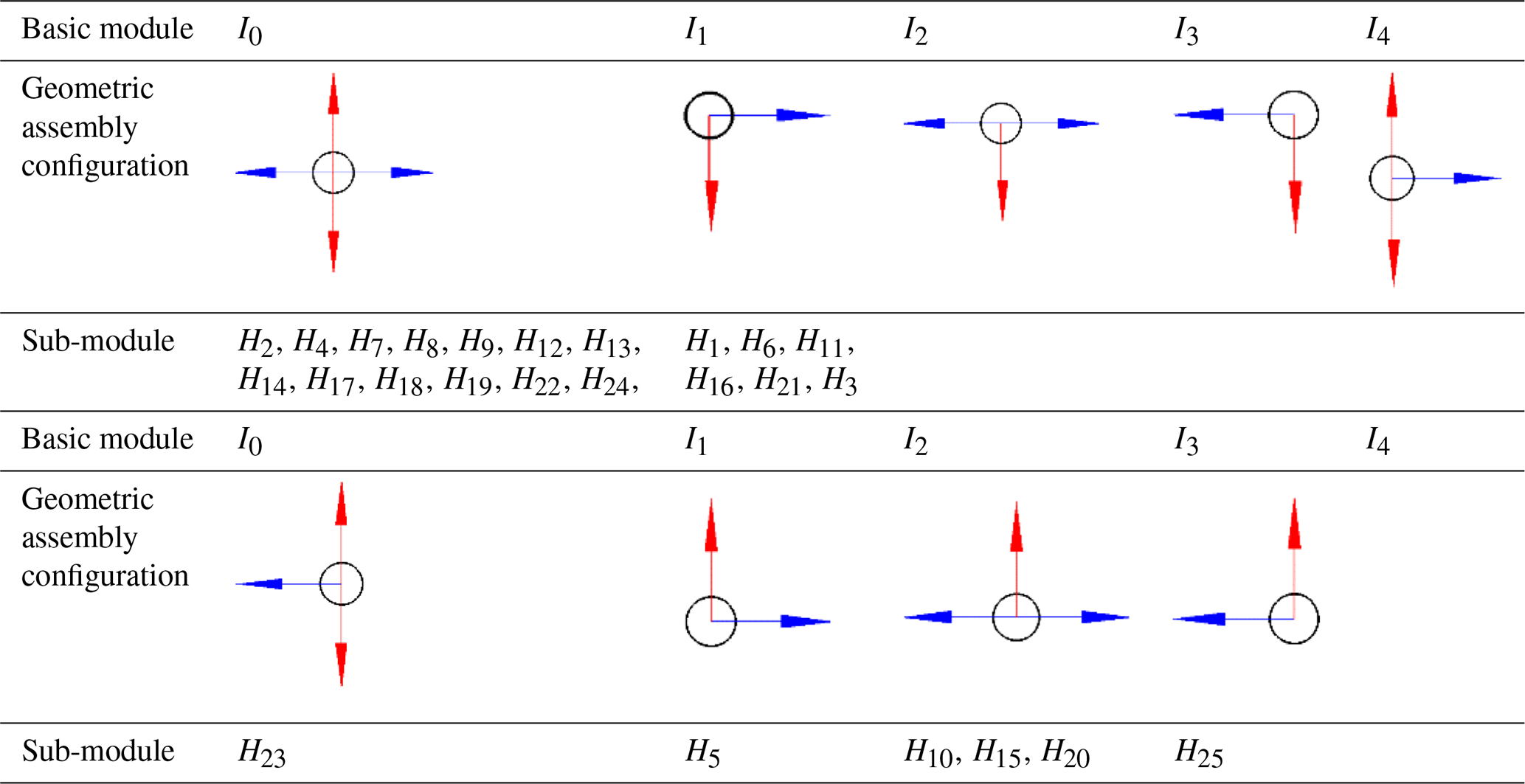
Based on the above analysis, the dynamic model of the large parabolic cylindrical deployable structure can be divided into 25 dynamic sub-modules, which are composed of 9 dynamic basic modules. I₁–I₈ are subsets of I₀; the geometric assembly configuration of the I₀ basic module shown in Fig. 8 is composed of two BUD sub-rings and two MBUG sub-rings. Figure 8 shows the geometric configuration of BUD and MBUG.

Figure 8 Basic module I₀.

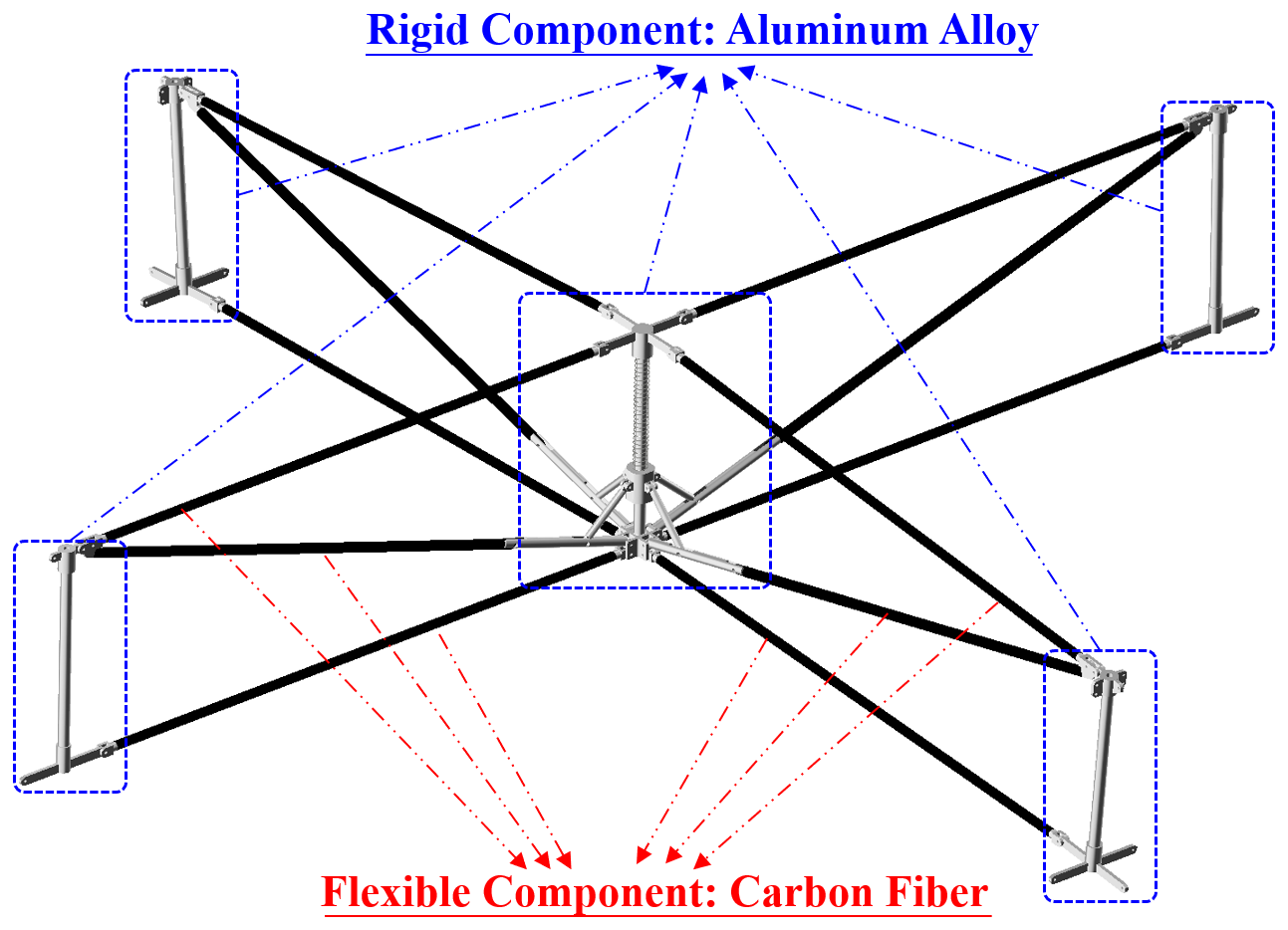
Both types of sub-rings use the NCF beam to divide rigid members (the blue lines in Fig. 9; the beam cross section is a circular section with a diameter of 25 mm), and the ANCF full-parameter beams are used to divide the flexible members (the red lines in Fig. 9; the cross-section is a ring, inner diameter is 18 mm, outer diameter is 20 mm). While considering the calculation accuracy and the calculation cost, this paper uses five ANCF beam elements to divide each flexible member. The physical parameters and geometric parameters of NCF and ANCF in the sub-ring are shown in Table 2.

Figure 9 Geometric configuration of BUD and MBUG. (a) BUD sub-ring. (b) MBUG sub-ring.

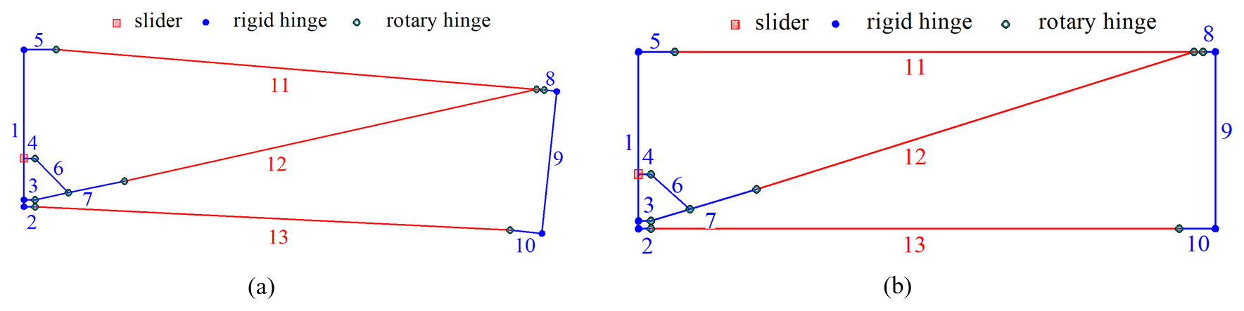
Table 2 Physical and geometric parameters.

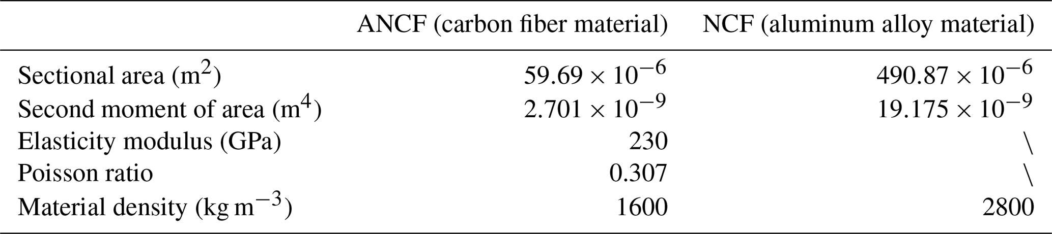
\: the NCF unit does not contain this parameter.

The rigid drive component and rigid connection component in the BUD and MBUG sub-rings are shown in Fig. 10 using the NCF element to divide the rigid drive component into seven beam elements $\left\{k^{\prime }k,c^{\prime }c,a^{\prime }a,f^{\prime }f,k^{\prime }{f}^{\prime },ab,cd\right\}$ and divide the rigid connection component into 3 beam elements $\left\{g^{\prime }g,h^{\prime }h,gh\right\}$. When establishing the dynamic equation, the mass of the slider is averagely attached to the endpoint of the adjacent NCF beam in the form of mass points.

Figure 10 Rigid components. (a) Rigid drive component. (b) Rigid connection component.

Because the slider slides on the vector corresponding to beam $k^{\prime }{f}^{\prime }$, the vector corresponding to beam ab always satisfies the following equation:

$$\begin{array}{}\text{(24)}& \cos \left(\mathit{\theta }\right)={\displaystyle \frac{{\mathit{r}}_{ab}\cdot {\mathit{r}}_{k^{\prime }{f}^{\prime }}}{\left|{\mathit{r}}_{ab}\right|\left|{\mathit{r}}_{k^{\prime }{f}^{\prime }}\right|}}.\end{array}$$

At the same time, θ needs to satisfy the following geometric equation:

$$\begin{array}{}\text{(25)}& \left\{\begin{array}{l}\cos \left(\mathit{\theta }\right)=\frac{{\stackrel{\mathrm{‾}}{ab}}^{\mathrm{2}}+{\stackrel{\mathrm{‾}}{ac}}^{\mathrm{2}}-{\stackrel{\mathrm{‾}}{kb}}^{\mathrm{2}}}{\mathrm{2}\cdot \stackrel{\mathrm{‾}}{ab}\cdot \stackrel{\mathrm{‾}}{ac}}\\ ac=x_{\mathrm{0}}\\ x_{\mathrm{0}}=\left|{\mathit{r}}_{\mathrm{a}}-{\mathit{r}}_{\mathrm{c}}\right|\end{array}\right..\end{array}$$

Equations (24) and (25) can describe the sliding constraint of the slider; the rotation hinge constraint Φ_rotaty and rigid connection constraint Φ_rigid contained in the sub-ring can be expressed as

$$\begin{array}{}\text{(26)}& \left\{\begin{array}{l}{\mathbf{\Phi }}_{\mathrm{rigid}}=\left\{\begin{array}{l}{\mathit{r}}_i-{\mathit{r}}_j=\mathrm{0}\\ {\mathit{r}}_{i,\mathit{\alpha }}\perp {\mathit{r}}_{j,\mathit{\beta }}\left(\mathit{\alpha }\ne \mathit{\beta },\mathit{\alpha },\mathit{\beta }=x,y,z\right)\end{array}\right.\\ {\mathbf{\Phi }}_{\mathrm{rotaty}}=\left\{\begin{array}{l}{\mathit{r}}_i-{\mathit{r}}_j=\mathrm{0}\\ {\mathit{r}}_{i,u}\perp {\mathit{r}}_{j,v},{\mathit{r}}_{i,u}\perp {\mathit{r}}_{j,w}\end{array}\right.\end{array}\right.,\end{array}$$

where i and j represent two nodes that are hinged or rigidly connected and ${\mathit{r}}_{i,\mathit{\alpha }}(\mathit{\alpha }=x,y,z)$ represents the local coordinate axis of the point i, the expression of the constraint equation in the absolute nodal coordinate method can be specifically found in the literature (Sugiyama et al., 2003). In order to avoid the Poisson lock effect of the ANCF beam element, Poisson's ratio is taken to be 0 in this paper, and then the dynamic equation of the I₀ basic module is established based on the ANCF-NCF method.

$$\begin{array}{}\text{(27)}& H_{\mathrm{0}}:\left\{\begin{array}{l}\left[\begin{array}{cc}{\mathbf{M}}^{\mathrm{g}}& \\ & {\mathbf{M}}^{\mathrm{r}}\end{array}\right]\left[\begin{array}{c}{\ddot{\mathbf{q}}}_{\mathrm{g}}\\ {\ddot{\mathbf{q}}}_{\mathrm{r}}\end{array}\right]+{\mathbf{\Phi }}_{\mathrm{q}}^{\mathrm{T}}\mathit{\lambda }+\left[\begin{array}{c}-{\mathbf{Q}}^{\mathrm{g}}\\ {\mathit{F}}^{\mathrm{r}}\left({\mathbf{q}}_{\mathrm{r}}\right)-{\mathbf{Q}}^{\mathrm{r}}\end{array}\right]=\mathbf{0}\\ \mathbf{\Phi }\left({\mathbf{q}}_{\mathrm{g}},{\mathbf{q}}_{\mathrm{r}},t\right)=\mathbf{0}\end{array}\right.,\end{array}$$

where M^g and M^r are the mass matrix of the rigid part and the flexible part; Q^g and Q^r are the generalized external force of the rigid part and the flexible part, respectively; F^r(q_r) is the elastic force of the flexible part; Φ(q_g and q_r,t) are the constraint equations; and λ is the corresponding Lagrange multiplier.

It can be seen from the above analysis that firstly, by establishing the dynamics basic module H₀ of I₀, we can then remove the corresponding generalized coordinates, mass matrix, constraint equation, and elastic force from the H₀ to obtain the dynamic basic modules of I₁–I₈; then, 25 dynamic sub-modules are obtained by transforming the generalized coordinate of I₁–I₈, finally assembling the overall dynamic equation of the deployable structure:

$$\begin{array}{}\text{(28)}& H_{\mathrm{TX}}=\underset{j=\mathrm{1}}{\overset{\mathrm{25}}{\bigwedge }}{\mathrm{\Omega }}_{jk}{\mathrm{\Theta }}_{k\mathrm{0}}{H}_{\mathrm{0}},\end{array}$$

where Θ_k0 represents moving the element from the I₀ dynamic basic module to the $I_k(k=\mathrm{1},\mathrm{\dots },\mathrm{8})$ dynamic basic module, Ω_jk represents the generalized coordinate element replacement from the I_k dynamic basic module to the $H_j(j=\mathrm{1},\mathrm{\dots },\mathrm{25})$ dynamic sub-module, and $\underset{j=\mathrm{1}}{\overset{\mathrm{25}}{\bigwedge }}$ represents the assembly of the 25 dynamic sub-modules equations.

2.4 Condensation and recursive algorithm for solving high-dimensional differential dynamics equations

The dynamic equations of large space flexible antennas with many identical sub-ring configurations can be rapidly achieved by the modular assembly method described in the third part. However, the final assembled dynamic equation has dimensions up to hundreds of thousands, such a high-dimensional nonlinear equation system is undoubtedly extremely difficult and time-consuming to solve. As mentioned in the introduction, the existing antenna dynamics analysis is often based on smaller deployable modules, and the dynamics research of large space deployable antennas needs to be studied further. Therefore, this paper proposes a new condensation and recursion algorithm module by module based on the modular assembly dynamics model.

The common solution methods of differential-algebraic equations include the Baumgarte method, Bathe integration strategy, Newmark method, and generalized-α method. Tian et al. (2010) comprehensively compared the advantages and disadvantages of various numerical solving algorithms. The Newmark algorithm was adopted in this paper to solve the differential-algebraic equations.

$$\begin{array}{}\text{(29)}& \left\{\begin{array}{l}\mathbf{M}{\ddot{\mathbf{q}}}_{n+\mathrm{1}}+{\mathbf{\Phi }}_{\mathrm{q}}^{\mathrm{T}}{\mathit{\lambda }}_{n+\mathrm{1}}+\left(\mathbf{F}\left({\mathbf{q}}_{n+\mathrm{1}}\right)-\mathbf{Q}\right)=\mathbf{0}\\ \mathbf{\Phi }\left({\mathbf{q}}_{n+\mathrm{1}},t_{n+\mathrm{1}}\right)=\mathbf{0}\end{array}\right.\end{array}$$

There, the following applies:

$$\begin{array}{}\text{(30)}& \left\{\begin{array}{l}{\mathbf{q}}_{n+\mathrm{1}}={\mathbf{q}}_n+h{\dot{\mathbf{q}}}_n+\frac{h^{\mathrm{2}}}{\mathrm{2}}\left[(\mathrm{1}-\mathrm{2}\mathit{\eta }){\ddot{\mathbf{q}}}_n+\mathrm{2}\mathit{\eta }{\ddot{\mathbf{q}}}_{n+\mathrm{1}}\right]\\ {\dot{\mathbf{q}}}_{n+\mathrm{1}}={\dot{\mathbf{q}}}_n+h\left[(\mathrm{1}-\mathit{\gamma }){\ddot{\mathbf{q}}}_n+\mathit{\gamma }{\ddot{\mathbf{q}}}_{n+\mathrm{1}}\right]\end{array}\right.,\end{array}$$

where η and γ are the algorithm parameters that determine the calculation accuracy and efficiency and h is the integration step size that is needed in order to make the algorithm stable, usually $\mathit{\gamma }\ge \mathrm{1}/\mathrm{2}$ and $\mathit{\eta }\ge (\mathit{\gamma }+\mathrm{1}/\mathrm{2}{)}^{\mathrm{2}}/\mathrm{4}$. Then, based on the Newmark method, taking the generalized acceleration and Lagrange multiplier as unknown variables, in the kth Newton iteration process, the following algebraic equations need to be solved:

$$\begin{array}{}\text{(31)}& {\left[\begin{array}{cc}\mathbf{M}+\frac{\partial \left(\mathbf{F}\left({\mathbf{q}}_{n+\mathrm{1}}\right)-\mathbf{Q}\right)}{\partial {\mathbf{q}}_{n+\mathrm{1}}}\mathit{\eta }{h}^{\mathrm{2}}& {\mathbf{\Phi }}_q^{\mathrm{T}}\\ \mathit{\eta }{h}^{\mathrm{2}}{\mathbf{\Phi }}_q& \mathbf{O}\end{array}\right]}^k{\left[\begin{array}{c}{\ddot{\mathbf{q}}}_{n+\mathrm{1}}\\ {\mathit{\lambda }}_{n+\mathrm{1}}\end{array}\right]}^k=-{\left[\begin{array}{c}{\mathbf{G}}_{\mathrm{1}}\\ {\mathbf{G}}_{\mathrm{2}}\end{array}\right]}^k.\end{array}$$

The following is also solved:

$$\begin{array}{}\text{(32)}& \left[\begin{array}{c}{\mathbf{G}}_{\mathrm{1}}\\ {\mathbf{G}}_{\mathrm{2}}\end{array}\right]=\left[\begin{array}{c}\mathbf{M}{\ddot{\mathbf{q}}}_{n+\mathrm{1}}+{\mathbf{\Phi }}_q^{\mathrm{T}}{\mathit{\lambda }}_{n+\mathrm{1}}+\left(\mathbf{F}\left({\mathbf{q}}_{n+\mathrm{1}}\right)-\mathbf{Q}\right)\\ \mathbf{\Phi }\left({\mathbf{q}}_{n+\mathrm{1}},t_{n+\mathrm{1}}\right)\end{array}\right].\end{array}$$

Therefore, the following applies:

$$\begin{array}{}\text{(33)}& {\left[\begin{array}{c}{\ddot{\mathbf{q}}}_{n+\mathrm{1}}\\ {\mathit{\lambda }}_{n+\mathrm{1}}\end{array}\right]}^{k+\mathrm{1}}={\left[\begin{array}{c}{\ddot{\mathbf{q}}}_{n+\mathrm{1}}\\ {\mathit{\lambda }}_{n+\mathrm{1}}\end{array}\right]}^k+{\left[\begin{array}{c}{\ddot{\mathbf{q}}}_{n+\mathrm{1}}\\ {\mathit{\lambda }}_{n+\mathrm{1}}\end{array}\right]}^k.\end{array}$$

Since the number of generalized coordinates and the number of constraint equations of the parabolic structure studied in this paper are very high, the dimension of the differential-algebraic Eq. (31) is very high, and the solution process is extremely time-consuming. Therefore, referring to the idea of static condensation, the generalized coordinates of the parabolic cylindrical deployable structure are divided into $\mathbf{q}=\left\{{\mathbf{q}}_j\mathrm{|}j=\mathrm{1},\mathrm{2},\mathrm{\dots },\mathrm{25}\right\}$, where q_j is the generalized coordinate in the H_j dynamic sub-module. The number of generalized coordinates in H_j is u, the number of constraint equations contained in H_j is s, and, the total number of generalized coordinates excluding H_j is v, the total number of constraint equations excluding H_j is t. Thus, Eq. (31) can be expressed in the following block matrix form:

$$\begin{array}{}\text{(34)}& \begin{array}{rl}& \left[\begin{array}{cc}\left[\begin{array}{cc}{\mathbf{K}}_{\mathrm{bb}}^{u\times u}& {\mathbf{K}}_{\mathrm{bi}}^{u\times v}\\ {\mathbf{K}}_{\mathrm{ib}}^{v\times u}& {\mathbf{K}}_{\mathrm{ii}}^{v\times v}\end{array}\right]& \left[\begin{array}{cc}{\left[{\mathbf{\Phi }}_{q_b}^b\right]}^{\mathrm{T}u\times s}& {\left[{\mathbf{\Phi }}_{q_b}^i\right]}^{\mathrm{T}u\times t}\\ {\left[{\mathbf{\Phi }}_{q_i}^b\right]}^{\mathrm{T}v\times s}& {\left[{\mathbf{\Phi }}_{q_i}^i\right]}^{\mathrm{T}v\times t}\end{array}\right]\\ \mathit{\eta }{h}^{\mathrm{2}}\left[\begin{array}{cc}{\left[{\mathbf{\Phi }}_{q_b}^b\right]}^{s\times u}& {\left[{\mathbf{\Phi }}_{q_i}^b\right]}^{s\times v}\\ {\left[{\mathbf{\Phi }}_{q_b}^i\right]}^{t\times u}& {\left[{\mathbf{\Phi }}_{q_i}^i\right]}^{t\times v}\end{array}\right]& \left[\begin{array}{cc}{\mathbf{O}}^{s\times s}& {\mathbf{O}}^{s\times t}\\ {\mathbf{O}}^{t\times s}& {\mathbf{O}}^{t\times t}\end{array}\right]\end{array}\right]\\ & \left[\begin{array}{c}\begin{array}{c}{\ddot{\mathbf{q}}}_b\\ {\ddot{\mathbf{q}}}_i\end{array}\\ \begin{array}{c}\mathrm{\Delta }{\mathit{\lambda }}_b\\ {\mathit{\lambda }}_i\end{array}\end{array}\right]=-\left[\begin{array}{c}\begin{array}{c}{\mathbf{G}}_{\mathrm{1}}^b\\ {\mathbf{G}}_{\mathrm{1}}^i\end{array}\\ \begin{array}{c}{\mathbf{G}}_{\mathrm{2}}^b\\ {\mathbf{G}}_{\mathrm{2}}^i\end{array}\end{array}\right].\end{array}\end{array}$$

Here, the following applies:

$$\begin{array}{}\text{(35)}& \mathbf{K}=\mathbf{M}+{\displaystyle \frac{\partial \left(\mathbf{F}\left({\mathbf{q}}_{n+\mathrm{1}}\right)-\mathbf{Q}\right)}{\partial {\mathbf{q}}_{n+\mathrm{1}}}}\mathit{\eta }{h}^{\mathrm{2}},\end{array}$$

In Eq. (34), the vector or matrix with the subscript b belongs to the condensation module, and the vector or matrix with the subscript i is the module to be polycondensation, which is reassembled into the block form as follows:

$$\begin{array}{}\text{(36)}& \begin{array}{rl}& \left[\begin{array}{cc}\left[\begin{array}{cc}{\mathbf{K}}_{\mathrm{bb}}^{u\times u}& {\left[{\mathbf{\Phi }}_{q_b}^b\right]}^{\mathrm{T}u\times s}\\ \mathit{\eta }{h}^{\mathrm{2}}{\left[{\mathbf{\Phi }}_{q_b}^b\right]}^{s\times u}& {\mathbf{O}}^{s\times s}\end{array}\right]& \left[\begin{array}{cc}{\mathbf{K}}_{\mathrm{bi}}^{u\times v}& {\left[{\mathbf{\Phi }}_{q_b}^i\right]}^{\mathrm{T}u\times t}\\ \mathit{\eta }{h}^{\mathrm{2}}{\left[{\mathbf{\Phi }}_{q_i}^b\right]}^{s\times v}& {\mathbf{O}}^{s\times t}\end{array}\right]\\ \left[\begin{array}{cc}{\mathbf{K}}_{\mathrm{ib}}^{v\times u}& {\left[{\mathbf{\Phi }}_{q_i}^b\right]}^{\mathrm{T}v\times s}\\ \mathit{\eta }{h}^{\mathrm{2}}{\left[{\mathbf{\Phi }}_{q_b}^i\right]}^{t\times u}& {\mathbf{O}}^{t\times s}\end{array}\right]& \left[\begin{array}{cc}{\mathbf{K}}_{\mathrm{ii}}^{v\times v}& {\left[{\mathbf{\Phi }}_{q_i}^i\right]}^{\mathrm{T}v\times t}\\ \mathit{\eta }{h}^{\mathrm{2}}{\left[{\mathbf{\Phi }}_{q_i}^i\right]}^{t\times v}& {\mathbf{O}}^{t\times t}\end{array}\right]\end{array}\right]\\ & \left[\begin{array}{c}\begin{array}{c}{\ddot{\mathbf{q}}}_b\\ {\mathit{\lambda }}_b\end{array}\\ \begin{array}{c}{\ddot{\mathbf{q}}}_i\\ {\mathit{\lambda }}_i\end{array}\end{array}\right]=-\left[\begin{array}{c}\begin{array}{c}{\mathbf{G}}_{\mathrm{1}}^b\\ {\mathbf{G}}_{\mathrm{2}}^b\end{array}\\ \begin{array}{c}{\mathbf{G}}_{\mathrm{1}}^i\\ {\mathbf{G}}_{\mathrm{2}}^i\end{array}\end{array}\right].\end{array}\end{array}$$

We introduce the following:

$$\begin{array}{}\text{(37)}& \left\{\begin{array}{c}{\mathbf{\Theta }}_{\mathrm{bb}}=\left[\begin{array}{cc}{\mathbf{K}}_{\mathrm{bb}}^{u\times u}& {\left[{\mathbf{\Phi }}_{q_b}^b\right]}^{\mathrm{T}u\times s}\\ \mathit{\eta }{h}^{\mathrm{2}}{\left[{\mathbf{\Phi }}_{q_b}^b\right]}^{s\times u}& {\mathbf{O}}^{s\times s}\end{array}\right],{\mathbf{\Theta }}_{\mathrm{ii}}=\left[\begin{array}{cc}{\mathbf{K}}_{\mathrm{ii}}^{v\times v}& {\left[{\mathbf{\Phi }}_{q_i}^i\right]}^{\mathrm{T}v\times t}\\ \mathit{\eta }{h}^{\mathrm{2}}{\left[{\mathbf{\Phi }}_{qi}^i\right]}^{t\times v}& {\mathbf{O}}^{t\times t}\end{array}\right]\\ {\mathbf{\Theta }}_{\mathrm{bi}}=\left[\begin{array}{cc}{\mathbf{K}}_{\mathrm{bi}}^{u\times v}& {\left[{\mathbf{\Phi }}_{q_b}^i\right]}^{\mathrm{T}u\times t}\\ \mathit{\eta }{h}^{\mathrm{2}}{\left[{\mathbf{\Phi }}_{q_i}^b\right]}^{s\times v}& {\mathbf{O}}^{s\times t}\end{array}\right],{\mathbf{\Theta }}_{\mathrm{ib}}=\left[\begin{array}{cc}{\mathbf{K}}_{\mathrm{ib}}^{v\times u}& {\left[{\mathbf{\Phi }}_{q_i}^b\right]}^{\mathrm{T}v\times s}\\ \mathit{\eta }{h}^{\mathrm{2}}{\left[{\mathbf{\Phi }}_{q_b}^i\right]}^{t\times u}& {\mathbf{O}}^{t\times s}\end{array}\right]\end{array}\right..\end{array}$$

Then, Eq. (36) is expressed as

$$\begin{array}{}\text{(38)}& \left[\begin{array}{cc}{\mathbf{\Theta }}_{\mathrm{bb}}& {\mathbf{\Theta }}_{\mathrm{bi}}\\ {\mathbf{\Theta }}_{\mathrm{ib}}& {\mathbf{\Theta }}_{\mathrm{ii}}\end{array}\right]\left[\begin{array}{c}{\mathbf{x}}_b\\ {\mathbf{x}}_i\end{array}\right]=\left[\begin{array}{c}{\mathbf{G}}_b\\ {\mathbf{G}}_i\end{array}\right].\end{array}$$

There, the following applies:

$$\begin{array}{}\text{(39)}& {\mathbf{x}}_b=\left[\begin{array}{c}{\ddot{\mathbf{q}}}_b\\ {\mathit{\lambda }}_b\end{array}\right],{\mathbf{x}}_i=\left[\begin{array}{c}{\ddot{\mathbf{q}}}_i\\ {\mathit{\lambda }}_i\end{array}\right],{\mathbf{G}}_b=\left[\begin{array}{c}{\mathbf{G}}_{\mathrm{1}}^b\\ {\mathbf{G}}_{\mathrm{2}}^b\end{array}\right],{\mathbf{G}}_i=\left[\begin{array}{c}{\mathbf{G}}_{\mathrm{1}}^i\\ {\mathbf{G}}_{\mathrm{2}}^i\end{array}\right].\end{array}$$

By condensing the unknown variables, we get

$$\begin{array}{}\text{(40)}& {\mathbf{x}}_b={\left({\mathbf{\Theta }}_{\mathrm{bb}}\right)}^{-\mathrm{1}}\left({\mathbf{G}}_b-{\mathbf{\Theta }}_{\mathrm{bi}}{\mathbf{x}}_i\right).\end{array}$$

Substituting back into Eq. (38), we can obtain the next matrix equation to be condensed:

$$\begin{array}{}\text{(41)}& {\mathbf{E}}_i{\mathit{x}}_i={\mathbf{P}}_i.\end{array}$$

Here, the following applies:

$$\begin{array}{}\text{(42)}& {\mathbf{E}}_i={\mathbf{\Theta }}_{\mathrm{ii}}-{\mathbf{\Theta }}_{\mathrm{ib}}{\left({\mathbf{\Theta }}_{\mathrm{bb}}\right)}^{-\mathrm{1}}{\mathbf{\Theta }}_{\mathrm{bi}},{\mathbf{P}}_i={\mathbf{G}}_i-{\mathbf{\Theta }}_{\mathrm{ib}}{\left({\mathbf{\Theta }}_{\mathrm{bb}}\right)}^{-\mathrm{1}}{\mathbf{G}}_b.\end{array}$$

Repeat the steps in Eqs. (34)–(40) to condense the dynamic basic module H₁–H₂₄ and then recursively solve each unknown variable. It is much more efficient and easier to solve the differential equation of the condensation module ${\mathit{x}}_b={\left({\mathbf{\Theta }}_{\mathrm{bb}}\right)}^{-\mathrm{1}}\left({\mathbf{G}}_b-{\mathbf{\Theta }}_{\mathrm{bi}}{\mathit{x}}_i\right)$, finally, by substituting the acceleration increment and the Lagrange multiplier increment back into Eq. (33), the dynamic differential equation of a large flexible multibody system can be solved.

3 Large parabolic cylindrical antenna deployment process control

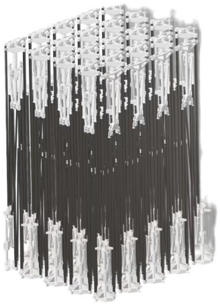
The closed configuration of the parabolic cylindrical antenna is shown in Fig. 11. In the fully retracted state, it is difficult to deploy the deployable antenna by the cylindrical springs distributed on the rigid drive component. Hence, the torsion spring distributed on the rotating hinge joint provides the driving force to expand the deployable structure from the fully closed position to the driving position, and then the cylindrical spring provides the driving force for deployment. The mechanical characteristics of the unfolding stage with the cylindrical spring force are exactly the research content of this paper.

Figure 11 Fully retracted state.

The deployable antenna has 25 driving springs with a spring stiffness of 6000 N m⁻¹. When the deployable structure is just unfolded to the driving position, the cylindrical spring force is 800 N. Therefore, the generalized external force of the deployable antenna is related to the slider position as follows:

$$\begin{array}{}\text{(43)}& \left\{{\mathbf{Q}}_z\left(\mathbf{s}\right)\left|Q_{\mathrm{zi}}\right.=-\left[\mathrm{800}-\mathrm{6000}\times (\mathrm{0.277}-s_i)\right],(i=\mathrm{1},\mathrm{\dots },\mathrm{25})\right\}.\end{array}$$

According to Fig. 6, s_i represents the distance of the slider relative to the local coordinate origin o, and the value of s_i decreases as the antenna expands. When in the driving position, the distance between the slider and origin o is 277 mm, and when expanded to the locked position, the distance between the slider and origin o is 160 mm. The large parabolic cylindrical antenna studied in this paper is passively deployed, and its deployment driving force is provided by cylindrical springs distributed on the rigid driving components. However, if the release rate of spring potential energy is not controlled, each component will suffer a severe impact. Therefore, it is necessary to control its unfolding process. Since the unfolding process of the deployable structure is only related to the travel of the slider, the deployment control of the structure is the control of the stroke of the slider. On the one hand, in order to ensure the stability of the parabolic cylindrical antenna during the deployment process, it is necessary to control the velocity peak of the slider in the process of deployment. On the other hand, at the end of the antenna deployment, the slider needs to have a certain velocity to achieve the self-locking in place, and at the same time, it is necessary to prevent the slider velocity from being too large to cause a great impact on the limit point and cause the overall instability of the antenna.

The proportion integral differential (PID) control algorithm is a common and effective control method in engineering; however, for the parabolic cylindrical antenna studied in this paper, due to its high nonlinearity and strong coupling, it is still difficult to obtain the ideal control effect by repeatedly adjusting the control parameters.

The parabolic cylindrical antenna designed based on the quadrilateral deployable mechanism shown in Fig. 6 requires a large driving force in the early stage of deployment but only a small driving force in the middle and late development. Therefore, it is difficult to realize the stable control of the mechanism according to the control scheme of linear feedback. Therefore, this paper constructs a slow-release force control function based on velocity feedback according to the idea of dynamic balance for this kind of strongly nonlinear and strong coupling system.

$$\begin{array}{}\text{(44)}& \mathit{u}\left(\mathit{s},\dot{\mathit{s}}\right)={\mathit{u}}_p\left(\mathit{s}\right)+{\mathit{u}}_{\mathrm{s}}\left(\dot{\mathit{s}}\right)\end{array}$$

$\mathit{u}\left(\mathit{s},\dot{\mathit{s}}\right)$ is the spring force that drives the slider; when the slider position of the deployable support reaches the critical value, the driving force required for deployment drops sharply, so the dynamic equilibrium state is constructed by introducing the spring force into the slow-release control function. ${\mathit{u}}_{\mathrm{s}}\left(\dot{\mathit{s}}\right)$ is the nonlinear feedback force related to the slider velocity $\dot{\mathit{s}}$, and its specific expression is as follows:

$$\begin{array}{}\text{(45)}& \begin{array}{rl}& \mathit{u}\left(\dot{\mathit{s}}\right)\\ & =\left\{\begin{array}{ll}\mathrm{150}\arctan \mathit{\{}-\mathrm{1000}[(\dot{\mathit{s}}+\mathrm{0.001})+\mathrm{0.035}\left]\mathit{\right\}}+\mathrm{232},& \dot{\mathit{s}}\le \mathrm{0}\\ \mathrm{150}\arctan \mathit{\{}-\mathrm{1000}[(\dot{\mathit{s}}+\mathrm{0.001})-\mathrm{0.02}\left]\mathit{\right\}}-\mathrm{227.6896},& \dot{\mathit{s}}>\mathrm{0}\end{array}\right..\end{array}\end{array}$$

According to the properties of the arctangent function, when the slider velocity reaches −0.035 and 0.02 m s⁻¹, the control force will increase or decrease abruptly. The relationship between ${\mathit{u}}_{\mathrm{s}}\left(\dot{\mathit{s}}\right)$ and the slider velocity can be shown in Fig. 12. The positioning of the driving sliders for the deployable parabolic cylindrical antenna support mechanism is illustrated in Fig. 13.

Figure 12 Feedback force.

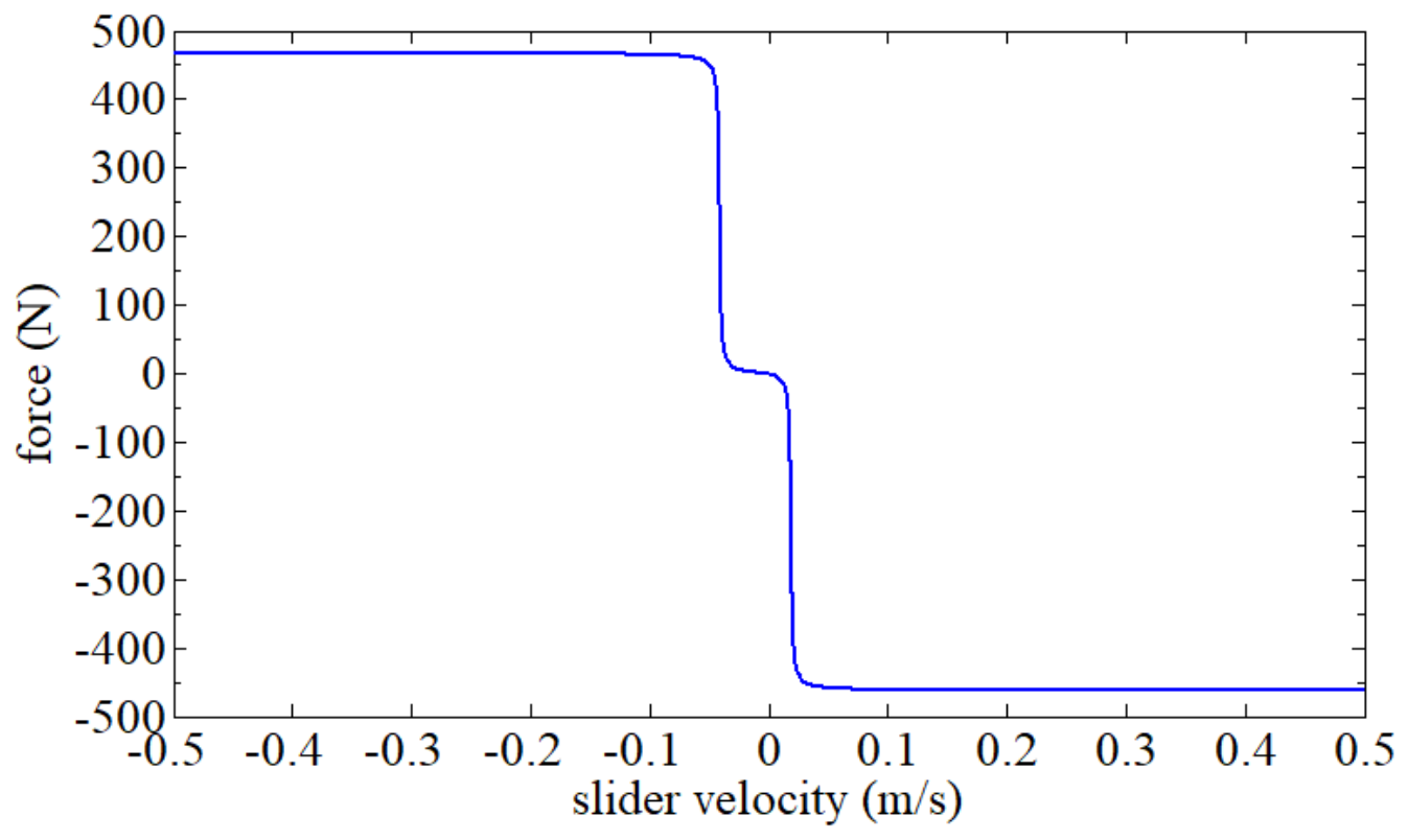
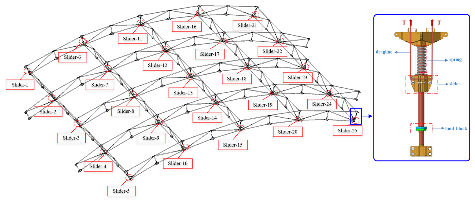
Figure 13 Deployment of the driving slider position and application of the release force are modulated.

4 Analysis results and discussions

4.1 Deployment dynamic analysis without control

According to the solution process in Sect. 2.4, the dynamic behavior of the parabolic cylindrical deployable structure during the deployment process can be solved.

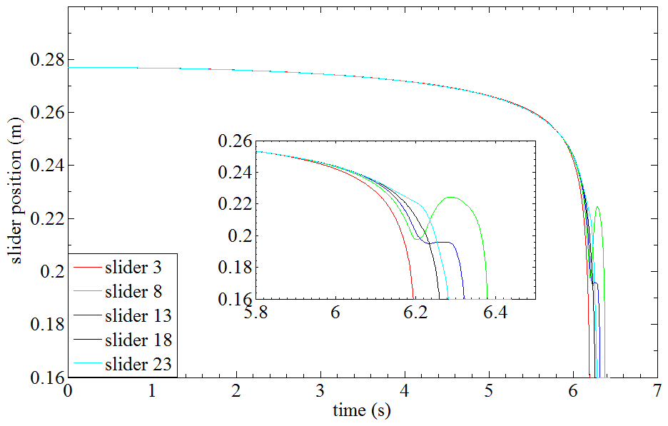
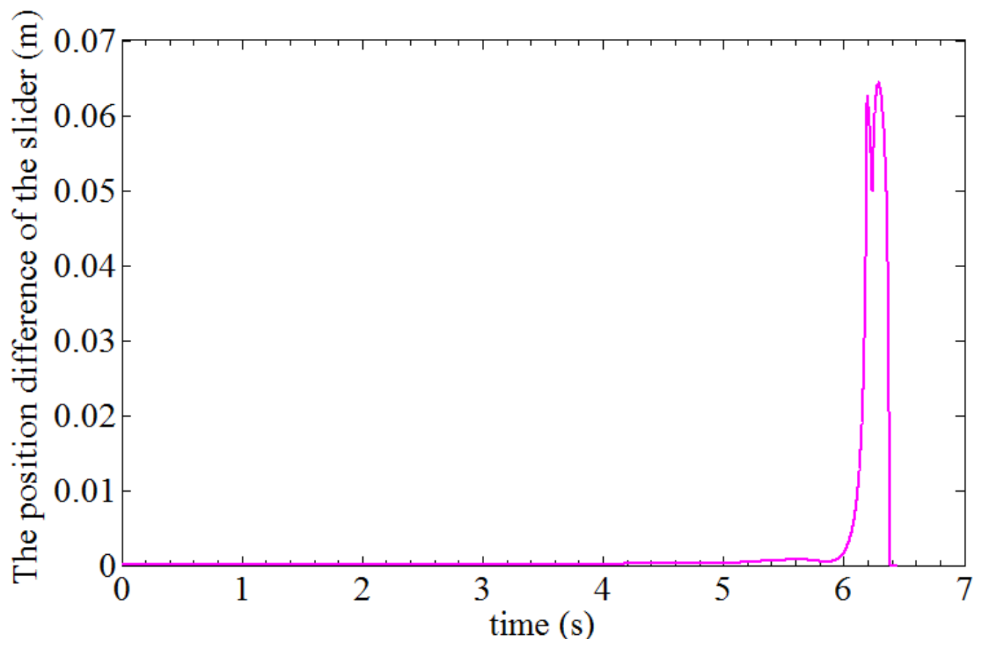
Figure 14 shows the position curves of sliders 3, 8, 13, 18, and 23, which are distributed in the middle of the first, second, third, fourth, and fifth cylinders, respectively (as can be seen in Fig. 13). It can be clearly seen that different cylinders of the deployable structure show great asynchronism in expansion when the antenna support mechanism expands to 5.9 s, and the first cylinder expands quickly, while the second one expands slowly. The maximum position difference between any two sliders in the whole process is shown in Fig. 15, which visually represents the expanded asynchrony of the structure in the deployment process. It can be seen from the results shown in the figure that the deployment asynchrony of the deployable support mechanism reaches a peak value of 64.38 mm at 6.285 s, and then the asynchrony decreases due to the gradual deployment of each cylinder until all the cylinders are deployed in place. According to the results shown in the figure, the deployment asynchrony reached the peak of 64.38 mm at 6.285 s; as each cylinder gradually unfolds into place, the asynchrony weakens and disappears.

Figure 14 Trajectories of sliders on different cylinders.

Figure 15 Maximum position difference between any two sliders.

The deployed configuration of the deployable structure when the slider position difference is the largest is shown in Fig. 16.

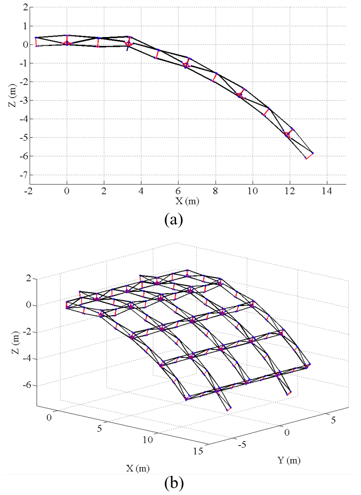
Figure 16 Configuration of the deployable structure, (a) Expanded configuration on the XZ plane, (b) Spatial expansion configuration.

From Fig. 16, it can be intuitively found that the second cylinder has poor synchronization and the lowest degree of expansion, and Fig. 17 shows the velocity curve of the slider on the second cylinder.

Figure 17 Velocity of the slider.

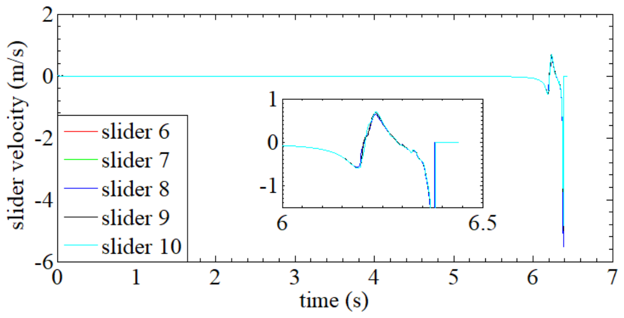
Here, a negative value of the slider velocity indicates an expanded state, and a positive value of the slider velocity shows the folding state. From the slider velocity trajectory, the parabolic cylindrical deployable structure studied in this paper has a very slow velocity growth in the first 6 s of the unfolding process, and the slider velocity on each cylinder is less than 0.1 m s⁻¹. At this point, the deployment position of each slider is around 0.24 m, which means 6 s before the deployment process the travel of the slider, it is only 0.028 m. Compared with the later stage of deployment, the travel of the slider reached 0.08 m in only 0.4 s. After 6 s, the velocity of each slider increases rapidly until each deployable support unit is deployed in place, and the maximum velocity of the slider reaches 5.508 m s⁻¹. Based on the above analysis, the deployable structure has a highly nonlinear unfolding process, and the slider velocity is too fast at the end of unfolding, which is enough to cause a great impact on the deployable structure when it is locked in place, affecting the stability of the antenna system.

4.2 Deployment dynamic analysis under velocity feedback control

Since the deployable support needs a large driving force in the early stage of deployment, the velocity feedback control force begins to apply when the slider velocity reaches 0.001 m s⁻¹. Then, according to the solution process shown in Sect. 2.4, the position trajectory of the slider on each rigid drive component can be obtained.

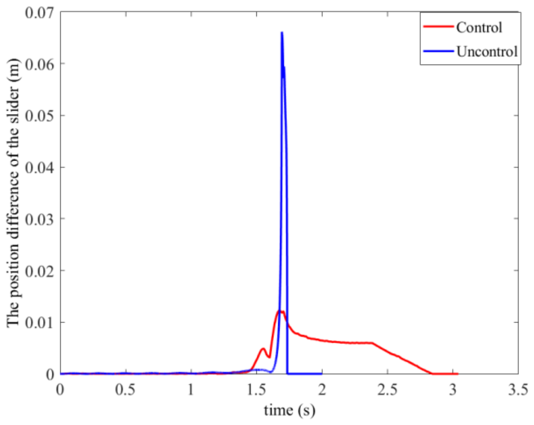
Figure 18 shows the position trajectories of the central sliders on the five cylinders under the action of the control force. It can be found that the deployment process of each slider slows down when it reaches the position of 0.22 m under the action of slow-release force. It can be seen from the figure that the third cylinder is first deployed in place, and the second cylinder is finally deployed in place. The asynchrony in the whole deployment process of the deployable structure can be represented by the maximum position difference between any two sliders, as shown in Fig. 19; according to the curve in the figure, when unfolded to 15.22 s, the deployment asynchrony reaches the maximum, with a peak value of 19.64 mm, which is 69.49 % lower than that without control force.

Figure 18 Trajectories of sliders on different cylinders.

Figure 19 Maximum position difference between any two sliders.

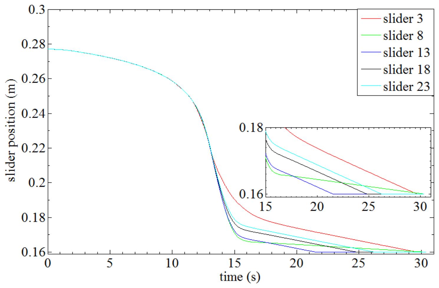
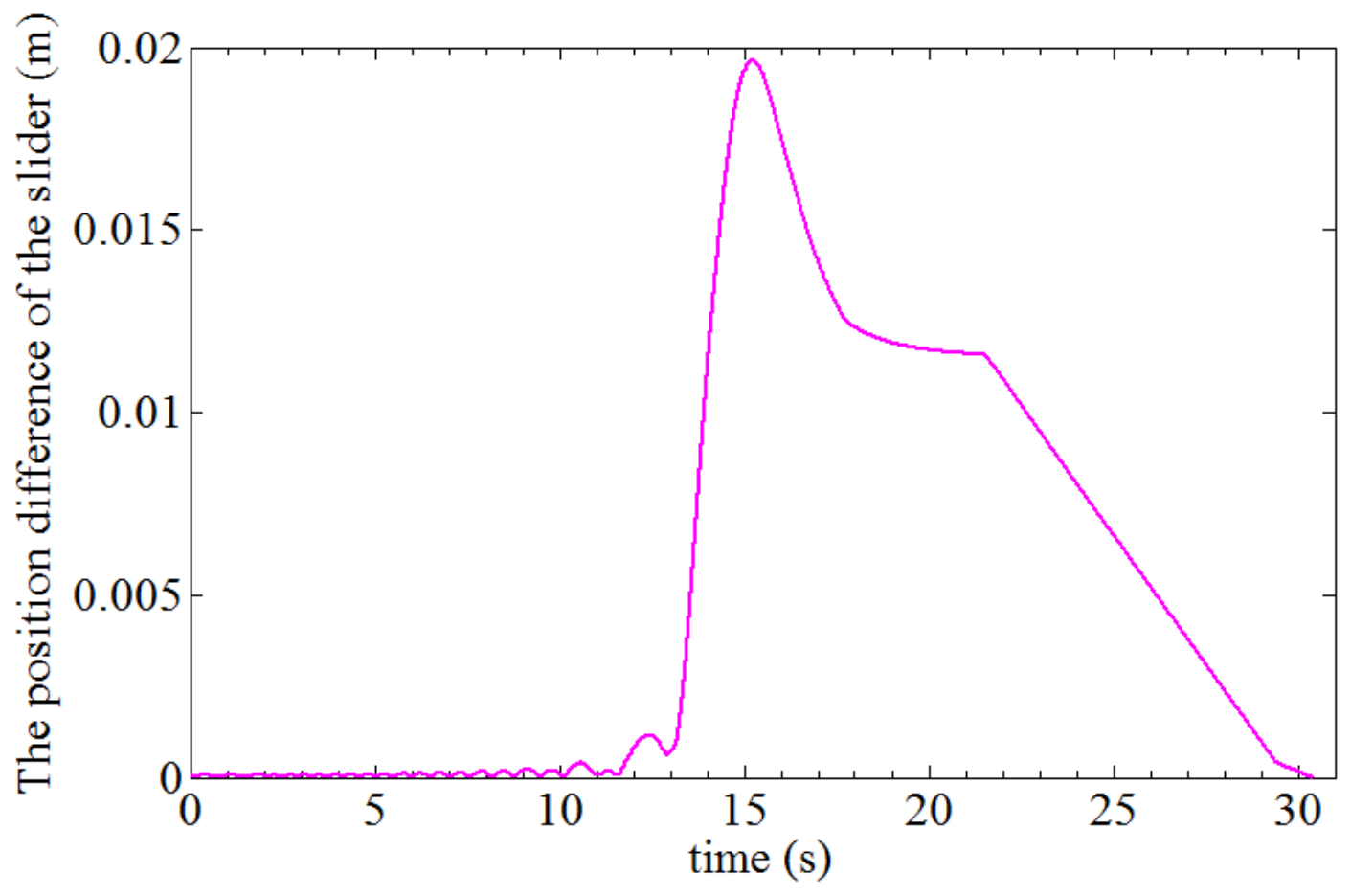
Figure 20 shows the velocity comparison curves of different cylinder center sliders of the deployable structure under the action of control force.

Figure 20 Sliders velocity on different cylinders.

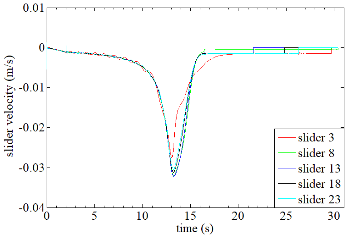
After the introduction of the control force, the velocity of each driving slider is greatly controlled, and it is obvious that the peak velocity of all sliders is less than 0.04 m s⁻¹, which greatly improves the stability of the deployable structure during deployment. And when each slider is deployed and in place, the slider velocity is less than 0.002 m s⁻¹, which greatly reduces the impact in the locking stage and ensures the stability of the antenna when it is locked. Based on the above analysis, the nonlinear control function proposed in this paper will significantly improve the deployable stability of the deployable structure. The control force curve of the second cylinder slider during the un-folding process is shown in Fig. 21.

Figure 21 Control force of the second cylinder slider.

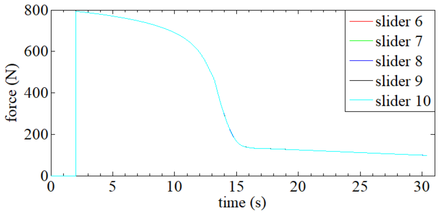
From the control force curve of each slider shown in Fig. 21, at about 2 s, the velocity of each slider gradually reaches 0.001 m s⁻¹, and the control force is generated. In order to see the change in ${\mathit{u}}_{\mathrm{s}}\left(\dot{\mathbf{s}}\right)$ more intuitively, the influence of the spring force is removed from the control force curve of the slider, and the remaining curve based on velocity feedback is shown as follows in Fig. 22.

Figure 22 Control force based on velocity feedback.

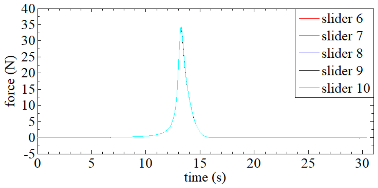
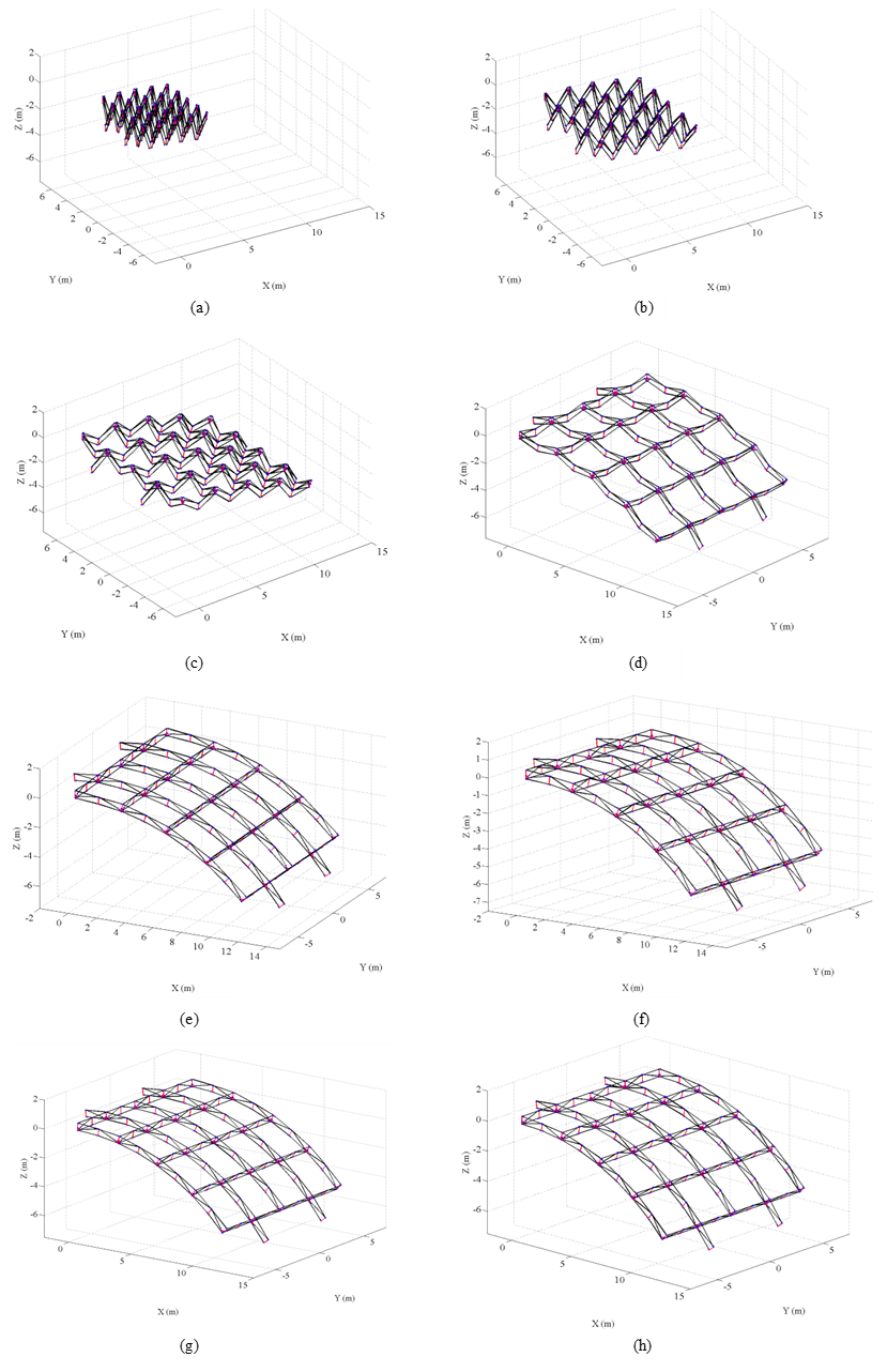
Figure 23 Deployed configuration: (a) 1 s, (b) 5 s, (c) 10 s, (d) 12.5 s, (e) 15 s, (f) 20 s, (g) 25 s, and (h) 30.4 s.

The curve after removing the spring force intuitively reflects the control force law required by the deployable antenna established based on the quadrilateral module shown in Fig. 6 during the deployment process. The control force increases sharply when the expansion degree of the quadrilateral expandable module reaches about 56 % and then decreases sharply. The whole deployment process shows a strong nonlinearity. The deployed configuration of the parabolic cylindrical deployable structure is shown in Fig. 23.

In Fig. 23, the velocity of the deployable parabolic cylindrical antenna varies rapidly at the beginning of the slider movement, with a slower rate of change in the later stages. There is a clear nonlinear relationship between the slider's deployment and the antenna's deployment.

4.3 Discussions

The current research mainly focuses on the dynamics of space deployable antennas and controlling the deployable process in peripheral deployable antennas. However, the study of large-scale back-shell deployable antennas with multi-closed-loop and strong coupling characteristics, such as the parabolic cylindrical antennas discussed in this paper, is still in the configuration design stage, and the research on the dynamics of the deployable process is still being broken through. The back-shell antenna has a complex structure with numerous supporting trusses and various types of joints. This complexity makes it difficult to establish the dynamics model, resulting in a large set of time-consuming equations. Based on existing research on the dynamics of flexible multibody systems, this paper proposes a modular modeling and an efficient dynamic solution method based on the condensation algorithm. It also constructs a nonlinear feedback control method for a dynamic equilibrium state.

For the uncontrolled and velocity feedback-based deployment process of the parabolic cylindrical deployable antenna, as shown by the maximum slider position difference curve in Fig. 24, it is evident that the dynamic balancing nonlinear feedback control strategy proposed in this paper significantly improves the synchronization of the antenna deployment, reduces the deployment velocity of the driving slider, and weakens the impact of the large slider velocity during locking on the support truss. Since space deployable antennas constitute a complex multibody system encompassing truss-type deployable support mechanisms and tensioned cable networks of reflective surfaces, extant research frequently overlooks the influence of the tensioned cable networks on the antenna deployment process. However, during actual in-orbit deployment, the pre-tension of the cable networks significantly impacts the deployment process. Moreover, in the final stages of antenna deployment, the pre-tension of the cable network acts as a resistive force, impeding the complete deployment of the antenna system and diminishing the precision of the reflective surface's shape. Consequently, in subsequent analyses of the dynamic characteristics of space deployable antenna deployment, it is imperative to thoroughly consider the influence of the pre-tension of the reflective surface's tensioned cable networks and to evaluate the reliability of in-orbit antenna deployment.

Figure 24 Comparison of asynchronicity in deployable antenna development.

5 Conclusion

This paper thoroughly studied the dynamic performance of large parabolic antenna support structure, proposed a modular dynamic assembly method for many components, and established a module-by-module condensation and recursive algorithm to solve the high-dimensional differential equation; this method has great reference value for this class of deployable truss antennas with many identical sub-rings. The main conclusions are as follows:

• 1.

  A modular method for assembling dynamic equations of a deployable antenna support structure with numerous components, which enables rapid construction of dynamic equations for flexible multibody systems with numerous identical sub-structures, has been proposed.

• 2.

  A high-dimensional differential equation computation method combining sequential polymerization and recursive solving, which significantly enhances the efficiency of solving high-dimensional dynamic differential equation systems, has been introduced.

• 3.

  The bilateral slow-release control method proposed for the deployment process of parabolic cylindrical antennas significantly improves synchronization during the deployment process, reducing the deployment asynchrony caused by structural flexibility by 69.49 %.

• 4.

  The feedback control method proposed in this paper reduces the peak deployment velocity of the parabolic cylindrical deployable antenna from 5.503 to 0.0323 m s⁻¹, effectively lowering the peak velocity of the drive slider during the deployment process. This results in a smaller slider velocity during the locking phase, weakening the impact on the deployable antenna and improving stability during the deployment process.

The research methodology in this paper can be further applied to studies on space solar arrays, space deployable manipulators, and other related fields.