Flexible manipulator trajectory tracking based on an improved adaptive particle swarm optimization algorithm with fuzzy PD control

Trajectory planning for flexible manipulators is a critical area of research in robotics. A trajectory tracking controller can enhance the accuracy of the manipulator's path and reduce vibrations. However, current flexible manipulators remain largely in the research phase, with many studies revealing issues such as poor accuracy in dynamic modeling, weak tracking performance in controller design, and insufficient vibration suppression capabilities. To address these challenges and improve the trajectory tracking performance of the manipulator, this paper focused on vibration suppression and trajectory planning for a two-link flexible manipulator and proposed a novel control method that integrates a modified adaptive particle swarm optimization algorithm (MAPSO) with fuzzy proportional–derivative (PD) control to achieve effective trajectory tracking. Firstly, the dynamic equations of the two-link flexible manipulator system were derived using the assumed modal method in conjunction with Lagrangian dynamics. Next, a 3-5-3 hybrid polynomial algorithm based on MAPSO was proposed to optimize the trajectory of the manipulator. Simulation results demonstrated that the optimization algorithm significantly enhances efficiency. Specifically, the number of iterations required for the two joints was reduced by 33 % and 54 %, respectively, when compared to the original algorithm. Additionally, this optimization led to a total reduction in running time of 0.03 s. Subsequently, the MAPSO algorithm was utilized to enhance the fuzzy PD controller based on the previously obtained optimal trajectory, leading to the development of a trajectory tracking controller known as MAPSO-FuzzyPD. Simulation results indicated that the proposed algorithm significantly reduced the maximum starting torque for both joints. Specifically, the maximum starting torque of joint 1 was decreased by 61.3 % and 40.3 % when compared to PD control and fuzzy PD control, respectively. Additionally, the maximum starting torque of joint 2 was reduced by 57.9 % and 42.1 % in comparison to the same control methods. Finally, an experimental platform for the flexible manipulator was established, and the experimental results further validated the effectiveness and feasibility of the algorithm proposed in this paper concerning joint trajectory tracking.

1 Introduction

In recent years, flexible manipulators have been widely adopted in aerospace, biomedical (Lee et al., 2012), and industrial applications (Yu et al., 2016). The trend in robotic arm systems is towards lighter, more complex, and more precise designs, making the influence of component flexibility increasingly significant. Traditional multi-rigid-body models often fail to accurately capture the dynamic characteristics of these flexible systems. Consequently, many researchers are focusing on the dynamic behavior of flexible multi-body systems. Meng et al. (2022) employed the assumed modal method (AMM) to model a rigid–flexible two-link manipulator. Similarly, Gao et al. (2019) utilized AMM to model a two-link flexible manipulator, demonstrating that their discrete model effectively mitigated data-related deficiencies, resulting in more stable outcomes. Sun et al. (2024a, b) combined AMM with the Lagrangian method to characterize the dynamics of a rigid–flexible coupled manipulator. Shen and Fan (2024) integrated AMM with the finite-element method (FEM) to investigate the dynamic characteristics of a flexible arm system using Bessel interpolation. Additionally, several scholars, such as Wang et al. (2010), Liu et al. (2017), Wang et al. (2017), Shao et al. (2020), and Alandoli et al. (2021), have employed FEM to derive dynamic equations by segmenting the arm into a finite number of elements. At this stage, most research on flexible robotic arms focuses on modeling in the horizontal plane, often neglecting the effects of gravity. However, in many practical applications where the robotic arm operates in a vertical plane, accounting for gravity becomes essential. Thus, it is crucial to incorporate gravitational factors into the dynamic modeling of flexible manipulators. By implementing the modal truncation technique within the assumed modal approach, the modal order of the system can be condensed into a finite-dimensional structure. This method effectively decreases the system's degrees of freedom and the quantity of equations required. Moreover, by employing the Lagrangian method to determine the disparity between the overall kinetic and potential energies of the system, the intricate internal force terms that typically complicate the computational procedure can be circumvented. This simplification not only alleviates the complexity of solving the dynamic equations but also streamlines the subsequent formation of the control system. Consequently, this investigation seeks to apply the assumed modal method and Lagrangian equations in delineating the deformation of a flexible arm and formulating the system's dynamic model.

Flexible manipulators are susceptible to vibrations and other issues during operation, leading to significant degradation in the positioning accuracy of the end effector. To address this, trajectory tracking often employs active vibration suppression control methods which aim to reduce or eliminate the structural vibration energy through active system control. Sasaki et al. (2023) utilized reinforcement learning to control the vibrations of a vertical-plane double-link flexible manipulator, designing a reward function to minimize the gap between the manipulator's end and the target coordinates. While this approach effectively suppressed vibrations, discrepancies were observed between simulation results and physical validation. He et al. (2021) developed a reinforcement learning controller for a horizontal two-link flexible manipulator using two neural networks: one for behavioral learning and the other for reward evaluation. Experimental verification demonstrated the controller's applicability. Reinforcement learning had also been used by Nageshrao et al. (2014) and Tang et al. (2014) to achieve control over target robotic arms. However, despite its promise, reinforcement learning has limitations, including high computational demands, extended training times, and requiring significant human intervention and optimization. Fuzzy control, on the other hand, is a widely adopted method known for its robustness and suitability for nonlinear systems. Numerous researchers have explored its applications. For instance, Alandoli et al. (2021) proposed a fuzzy logic control linear quadratic regulator (FLC-LQR) controller that combines optimal and fuzzy control strategies for a single-link flexible robotic arm, demonstrating effective vibration suppression and high robustness to uncertainties. Additionally, Beata (2018) introduced a fuzzy controller in a computer model of a rotating robotic arm joint with a localization control strategy, aimed at enhancing system performance by replacing traditional external controllers.

Traditional proportional–integral–derivative (PID) control is known for its simplicity and ease of implementation; however, its accuracy can decline when applied to complex systems. Integrating fuzzy control technology can enhance the capabilities of the original PID controller. Research by Anavatti et al. (2006), Liu et al. (2014), Zhang et al. (2016), and Chhabra et al. (2019) demonstrated the optimization of PID controllers through fuzzy control, with experimental evidence supporting the superiority of this combined approach. Despite its advantages, fuzzy control has limitations, particularly in its reliance on empirical design. The affiliation functions often require initial values that are determined through empirical and experimental methods. To address these drawbacks, Zhang et al. (2019) proposed a novel control scheme for a 3-degree-of-freedom robotic arm, utilizing a fuzzy proportional–derivative (PD) controller enhanced by a backpropagation neural network (BPNNBF-PD). This approach leverages the backpropagation neural network to calibrate the affiliation functions and optimize the performance of the fuzzy PD controller. In summary, while many researchers have explored fuzzy control, most have not fully mitigated its inherent drawbacks. Furthermore, there is a notable scarcity of studies focused on optimizing fuzzy PID controllers specifically for flexible manipulator applications.

The research direction of this paper is the vibration suppression trajectory planning and tracking control of a two-link flexible robotic arm, and a control method combining the improved particle swarm optimization algorithm with the fuzzy PD control is proposed to reach the purpose of trajectory tracking. Firstly, the dynamical equations of the robotic arm are obtained by assuming the modal method and the Lagrangian method on the non-inertial system. Then, a 3-5-3 hybrid polynomial algorithm based on the modified adaptive particle swarm optimization (MAPSO) is proposed to optimize the trajectory of the robotic arm. Finally, the MAPSO algorithm is utilized to modify the fuzzy PD controller on the basis of the obtained optimal trajectory to construct the MAPSO-FuzzyPD-based trajectory tracking controller, and the feasibility and superiority of the proposed method are demonstrated by theoretical and experimental analysis, respectively.

The focus of this paper is on vibration suppression, trajectory planning, and tracking control for a two-link flexible manipulator. A control method that combines an improved particle swarm optimization algorithm with fuzzy PD control was proposed to achieve effective trajectory tracking. Initially, the dynamic equations of the manipulator were derived using the modal method and the Lagrangian approach within a non-inertial reference frame. Subsequently, a 3-5-3 hybrid polynomial algorithm based on the MAPSO algorithm was introduced to optimize the trajectory of the robotic arm. Finally, the MAPSO algorithm was employed to refine the fuzzy PD controller based on the optimal trajectory obtained, resulting in the development of the MAPSO-FuzzyPD trajectory tracking controller. The feasibility and superiority of the proposed method were validated through both theoretical and experimental analyses.

2 Dynamic modeling of the flexible manipulator

2.1 Flexible manipulator model

The physical object of the flexible manipulator studied in this paper is illustrated in Fig. 1a. This flexible robotic arm system consists of two flexible connecting rods, and its mathematical model is depicted in Fig. 1b. The parameters of the flexible manipulator are shown in Table 1.

Figure 1 The flexible manipulator model. (a) The physical model. (b) The mathematical model.

Table 1 The main parameters of the flexible manipulator.

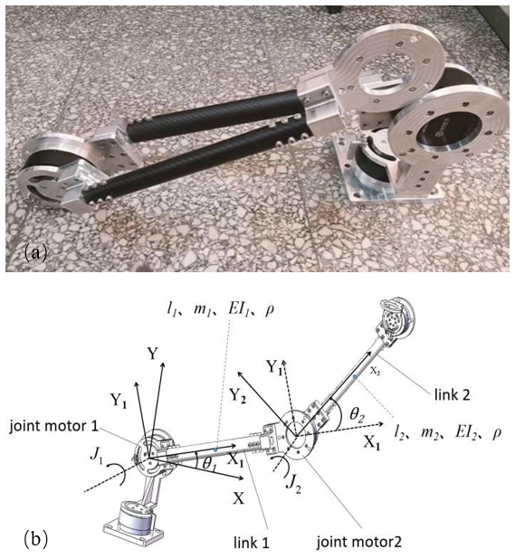
To facilitate the modeling of the system dynamics, the following assumptions were made:

• 1.

  The influence of joint flexibility was neglected, and only the flexibility of the connecting rods was considered in the vibration analysis and control studies.

• 2.

  The analysis focused solely on the bending deformation of the flexible connecting rods, while shear deformation and axial tensile/compressive deformation were ignored.

• 3.

  The deformations of the end load and the joint motor components of the robotic arm were considered small enough to disregard their effects on the overall system, treating them as mass points.

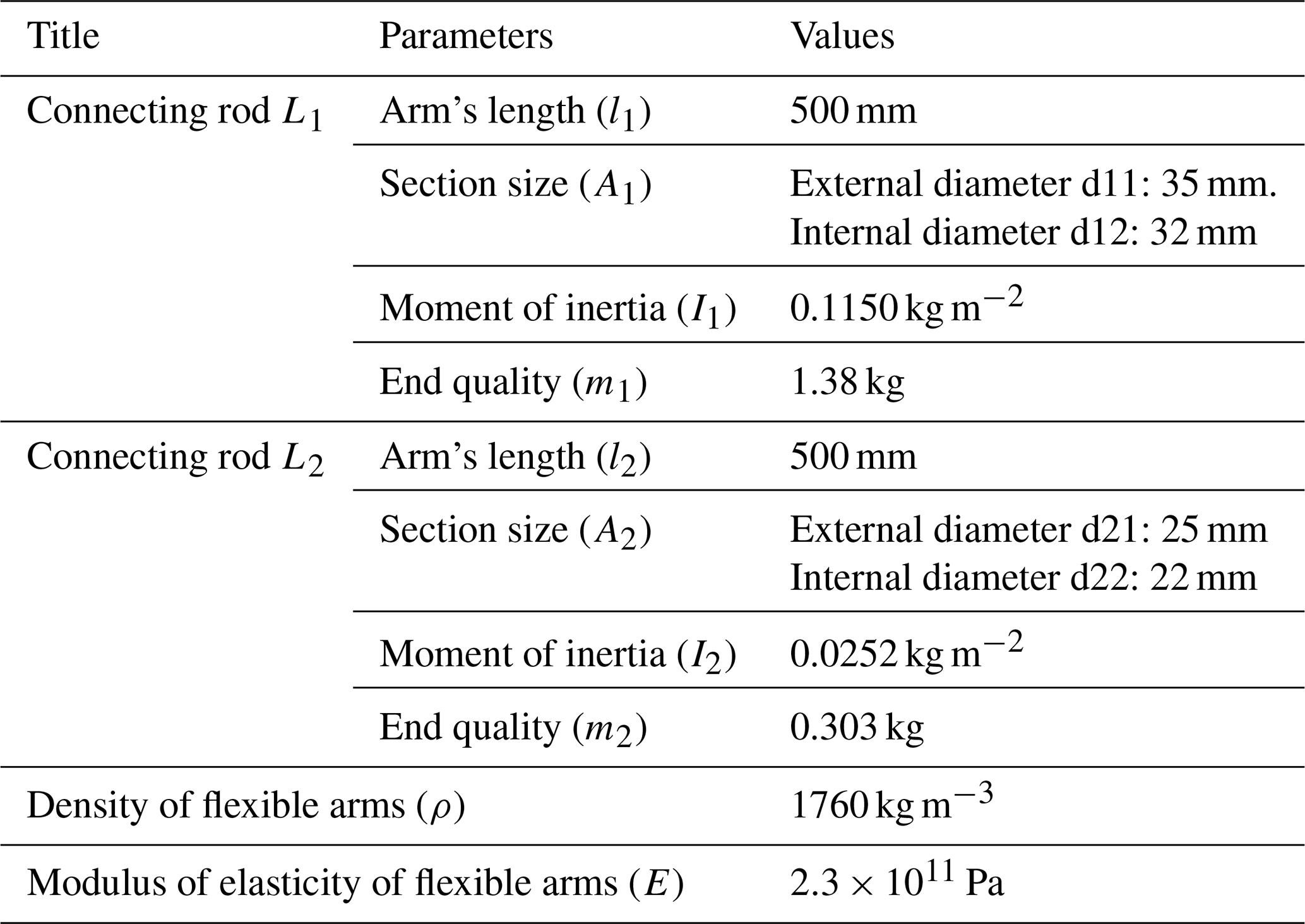
Based on the above assumptions, the coordinate system depicted in Fig. 2 was established. In this system, O–XY represents the inertial coordinate system, while O₁–X₁Y₁ and O₂–X₂Y₂ are the floating coordinate systems defined at the rotating joints of the flexible linkages L₁ and L₂, respectively. And here, r₁ denotes the position vector of the point corresponding to the transverse coordinate x₁ $(\mathrm{0}\le x_{\mathrm{1}}\le l_{\mathrm{1}})$ of the link L₁ with respect to the origin O of the inertial system. Similarly, r₂ represents the position vector of the point corresponding to the transverse coordinate x₂ $(\mathrm{0}\le x_{\mathrm{2}}\le l_{\mathrm{2}})$ of the link L₂ with respect to the origin O of the inertial system.

Figure 2 Coordinate system of the 2-degree-of-freedom flexible manipulator.

2.2 Dynamic modeling of the flexible manipulator

According to the assumed modal method, the vibration mode function of the flexible manipulator (Tavasoli, 2018) could be expressed as

$$\begin{array}{}\text{(1)}& w_i(x_i,t)={\sum }_{i=\mathrm{1}}^n{\mathrm{\Phi }}_i\left(x_i\right)q_i\left(t\right),\end{array}$$

where n is the number of retained modes, Φ_i(x_i) is the nth-order modal function of link i, q_i(t) represents the corresponding modal coordinate, and x_i denotes the axial position coordinate in the floating coordinate system of the link i.

Considering the two flexible connecting rods to be Euler–Bernoulli beams, the transverse vibration equations of motion can be expressed as (Omidi and Mahmoodi, 2016)

$$\begin{array}{}\text{(2)}& EI{\displaystyle \frac{{\partial }^{\mathrm{4}}w}{{\partial }^{\mathrm{4}}x}}+\mathit{\rho }A{\displaystyle \frac{{\partial }^{\mathrm{2}}w}{\partial t^{\mathrm{2}}}}=\mathrm{0}.\end{array}$$

According to the characteristics of the beam, the boundary conditions (Zhang et al., 2023) are defined as follows:

$$\begin{array}{}\text{(3)}& \left\{\begin{array}{l}{w}_i(\mathrm{0},t)=\mathrm{0},\\ \frac{\partial w_i(\mathrm{0},t)}{\partial x_i}=\mathrm{0},\\ E_i{I}_i\frac{{\partial }^{\mathrm{2}}{w}_i\left(l_i,t\right)}{{\partial }^{\mathrm{2}}{x}_i}=\mathrm{0},\\ E_i{I}_i\frac{{\partial }^{\mathrm{3}}{w}_i\left(l_i,t\right)}{{\partial }^{\mathrm{3}}{x}_i}=m_{\mathrm{end}}\frac{{\partial }^{\mathrm{2}}{w}_i\left(l_i,t\right)}{{\partial }^{\mathrm{2}}t}.\end{array}\right.\end{array}$$

The frequency equation, modal function, and intrinsic frequency of the beam are obtained by substituting Eq. (3) into Eq. (1), leading to the following results:

$$\begin{array}{}\text{(4)}& \begin{array}{rl}& \mathrm{1}+\cosh \left({\mathit{\lambda }}_{j}l\right)\cos \left({\mathit{\lambda }}_{j}l\right)\\ & ={\displaystyle \frac{m_{\mathrm{end}}}{m}}{\mathit{\lambda }}_{j}l(\sin \left({\mathit{\lambda }}_{j}l\right)\cosh \left({\mathit{\lambda }}_{j}l\right)-\cos \left({\mathit{\lambda }}_{j}l\right)\sinh \left({\mathit{\lambda }}_{j}l\right)),\end{array}\end{array}$$

$$\begin{array}{}\text{(5)}& \begin{array}{rl}& {\mathrm{\Phi }}_i\left(x_i\right)=\cosh \left({\mathit{\lambda }}_j{x}_i\right)-\cos \left({\mathit{\lambda }}_j{x}_i\right)\\ & -{\displaystyle \frac{\cosh \left({\mathit{\lambda }}_j{l}_{\mathrm{1}}\right)+\cos \left({\mathit{\lambda }}_j{l}_{\mathrm{1}}\right)}{\sinh \left({\mathit{\lambda }}_j{l}_{\mathrm{1}}\right)+\sin \left({\mathit{\lambda }}_j{l}_{\mathrm{1}}\right)}}\left(\sinh \left({\mathit{\lambda }}_j{x}_{\mathrm{1}}\right)-\sin \left({\mathit{\lambda }}_j{x}_{\mathrm{1}}\right)\right),\end{array}\end{array}$$

$$\begin{array}{}\text{(6)}& {\mathit{\omega }}_i={\mathit{\lambda }}_i^{\mathrm{2}}\sqrt{\left(E_i{I}_i\right)/\left({\mathit{\rho }}_i{A}_i\right)},\end{array}$$

where m is the mass of the flexible arm, m_end is the mass of the end of the flexible arm, and λ_j is the coefficient corresponding to the jth natural frequency.

According to our team's previous study, it is known that the first-order modes of this flexible manipulator play a major role in the deformation of the end elastic vibration. Therefore, the first-order modes were taken into account to calculate the dynamics model.

According to the geometric relationship, r₁ and r₂ can be expressed as

$$\begin{array}{}\text{(7)}& {\mathit{r}}_{\mathrm{1}}=\left[\begin{array}{l}{x}_{\mathrm{1}}{c}_{\mathrm{1}}-w_{\mathrm{1}}\left(x_{\mathrm{1}},t\right)s_{\mathrm{1}}\\ x_{\mathrm{1}}{s}_{\mathrm{1}}+w_{\mathrm{1}}\left(x_{\mathrm{1}},t\right)c_{\mathrm{1}}\end{array}\right],\end{array}$$

$$\begin{array}{}\text{(8)}& {\mathit{r}}_{\mathrm{2}}=\left[\begin{array}{l}{l}_{\mathrm{1}}{c}_{\mathrm{1}}-w_{\mathrm{1}}\left(l_{\mathrm{1}},t\right)s_{\mathrm{1}}+x_{\mathrm{2}}{c}_{\mathrm{12}}-w_{\mathrm{2}}\left(x_{\mathrm{2}},t\right)s_{\mathrm{12}}\\ l_{\mathrm{1}}{s}_{\mathrm{1}}+w_{\mathrm{1}}\left(l_{\mathrm{1}},t\right)c_{\mathrm{1}}+x_{\mathrm{2}}{s}_{\mathrm{12}}+w_{\mathrm{2}}\left(x_{\mathrm{2}},t\right)c_{\mathrm{12}}\end{array}\right],\end{array}$$

where c₁=cos θ₁, s₁=sin θ₁, $c_{\mathrm{12}}=\cos \left({\mathit{\theta }}_{\mathrm{1}}+{\mathit{\theta }}_{\mathrm{2}}\right)$, and $s_{\mathrm{12}}=\sin \left({\mathit{\theta }}_{\mathrm{1}}+{\mathit{\theta }}_{\mathrm{2}}\right)$.

To solve the kinetic equations, the Lagrangian method was used, the expression of which is as follows:

$$\begin{array}{}\text{(9)}& {\displaystyle \frac{\mathrm{d}}{\mathrm{d}t}}\left({\displaystyle \frac{\partial L}{\partial \dot{p}}}\right)-{\displaystyle \frac{\partial L}{\partial p}}=Q,\end{array}$$

where the Lagrangian function is given by $L=T-U$, T being the total kinetic energy of the system and U the total potential energy of the system. p denotes the generalized coordinate of the system, and Q is the generalized force in generalized coordinates.

The total kinetic energy (T) of this manipulator system consisted of the kinetic energy (T_G) generated by the motion of the system itself and the kinetic energy (T_i) generated by the elastic deformation of the flexible linkage. The kinetic energy of the system could be defined as

$$\begin{array}{}\text{(10)}& T=T_{\mathrm{G}}+T_i,\end{array}$$

$$\begin{array}{}\text{(11)}& \begin{array}{rl}{T}_{\mathrm{G}}& ={\displaystyle \frac{\mathrm{1}}{\mathrm{2}}}{J}_{\mathrm{0}}{\dot{{\mathit{\theta }}_{\mathrm{0}}}}^{\mathrm{2}}+{\displaystyle \frac{\mathrm{1}}{\mathrm{2}}}{m}_{\mathrm{0}}{l}_{\mathrm{0}}^{\mathrm{2}}{\dot{{\mathit{\theta }}_{\mathrm{0}}}}^{\mathrm{2}}+{\displaystyle \frac{\mathrm{1}}{\mathrm{2}}}{J}_{\mathrm{1}}{\left(\dot{{\mathit{\theta }}_{\mathrm{0}}}+\dot{{\mathit{\theta }}_{\mathrm{1}}}\right)}^{\mathrm{2}}\\ & +{\displaystyle \frac{\mathrm{1}}{\mathrm{2}}}{m}_{\mathrm{1}}{\left(\dot{{\mathit{r}}_{\mathrm{1}}}{\mathrm{|}}_{x_{\mathrm{1}}=l_{\mathrm{1}}}\right)}^{\mathrm{2}}+{\displaystyle \frac{\mathrm{1}}{\mathrm{2}}}{J}_{\mathrm{2}}{\left(\dot{{\mathit{\theta }}_{\mathrm{0}}}+\dot{{\mathit{\theta }}_{\mathrm{1}}}+\dot{{\mathit{\theta }}_{\mathrm{2}}}\right)}^{\mathrm{2}}\\ & +{\displaystyle \frac{\mathrm{1}}{\mathrm{2}}}{m}_{\mathrm{2}}{\left(\dot{{\mathit{r}}_{\mathrm{2}}}{\mathrm{|}}_{x_{\mathrm{2}}=l_{\mathrm{2}}}\right)}^{\mathrm{2}},\end{array}\end{array}$$

$$\begin{array}{}\text{(12)}& T_i={\displaystyle \frac{\mathrm{1}}{\mathrm{2}}}{\int }_{\mathrm{0}}^{l_{\mathrm{1}}}{\mathit{\rho }}_{\mathrm{1}}{A}_{\mathrm{1}}\dot{{\mathit{r}}_{\mathrm{1}}}\cdot \dot{{\mathit{r}}_{\mathrm{1}}}\mathrm{d}{x}_{\mathrm{1}}+{\displaystyle \frac{\mathrm{1}}{\mathrm{2}}}{\int }_{\mathrm{0}}^{l_{\mathrm{2}}}{\mathit{\rho }}_{\mathrm{2}}{A}_{\mathrm{2}}\dot{{\mathit{r}}_{\mathrm{2}}}\cdot \dot{{\mathit{r}}_{\mathrm{2}}}\mathrm{d}{x}_{\mathrm{2}}.\end{array}$$

The total elastic potential energy (U) of the manipulator system can be expressed as the sum of the gravitational potential energy (U_G) and the elastic potential energy (U_i) due to deformation. Thus, we can write the following:

$$\begin{array}{}\text{(13)}& U=U_{\mathrm{G}}+U_i,\end{array}$$

$$\begin{array}{}\text{(14)}& \begin{array}{rl}{U}_{\mathrm{G}}& =\left(m_{\mathrm{0}}+m_{\mathrm{1}}+m_{\mathrm{2}}\right)g{L}_{\mathrm{0}}{s}_{\mathrm{0}}\\ & +\left(m_{\mathrm{1}}+m_{\mathrm{2}}\right)g{L}_{\mathrm{1}}{s}_{\mathrm{01}}+m_{\mathrm{2}}g{L}_{\mathrm{2}}{s}_{\mathrm{012}},\end{array}\end{array}$$

$$\begin{array}{}\text{(15)}& \begin{array}{rl}{U}_i& ={\displaystyle \frac{\mathrm{1}}{\mathrm{2}}}{\sum }_{n=\mathrm{1}}^{\mathrm{2}}{\int }_{\mathrm{0}}^{l_i}{E}_i{I}_i{\left({\displaystyle \frac{{\partial }^{\mathrm{2}}{w}_i\left(x_i,t\right)}{\partial x_i^{\mathrm{2}}}}\right)}^{\mathrm{2}}\mathrm{d}{x}_i\\ & ={\displaystyle \frac{\mathrm{1}}{\mathrm{2}}}{K}_{\mathrm{1}}{q}_{\mathrm{1}}^{\mathrm{2}}+{\displaystyle \frac{\mathrm{1}}{\mathrm{2}}}{K}_{\mathrm{2}}{q}_{\mathrm{2}}^{\mathrm{2}},\end{array}\end{array}$$

where

$$\begin{array}{rl}& K_{\mathrm{1}}=E_{\mathrm{1}}{I}_{\mathrm{1}}{\int }_{\mathrm{0}}^{l_{\mathrm{1}}}{\left({\displaystyle \frac{{\partial }^{\mathrm{2}}{\mathrm{\Phi }}_{\mathrm{1}}\left(x_{\mathrm{1}}\right)}{\partial x_{\mathrm{1}}^{\mathrm{2}}}}\right)}^{\mathrm{2}}\mathrm{d}{x}_{\mathrm{1}},\\ & K_{\mathrm{2}}=E_{\mathrm{2}}{I}_{\mathrm{2}}{\int }_{\mathrm{0}}^{l_{\mathrm{2}}}{\left({\displaystyle \frac{{\partial }^{\mathrm{2}}{\mathrm{\Phi }}_{\mathrm{2}}\left(x_{\mathrm{2}}\right)}{\partial x_{\mathrm{2}}^{\mathrm{2}}}}\right)}^{\mathrm{2}}\mathrm{d}{x}_{\mathrm{2}}.\end{array}$$

The generalized coordinates are given as $p={\left({\mathit{\theta }}_{\mathrm{1}},{\mathit{\theta }}_{\mathrm{2}},q_{\mathrm{1}},q_{\mathrm{2}}\right)}^T$, where θ₁ and θ₂ denote the rigidity angles that the flexible linkage turns through and q₁ and q₂ are the modal coordinates of the flexible linkage. And the generalized force is $Q={\left({\mathit{\tau }}_{\mathrm{1}},{\mathit{\tau }}_{\mathrm{2}},\mathrm{0},\mathrm{0}\right)}^T$. Neglecting the coupling terms for the productization and the difference categories in the trigonometric equation, the kinetic expression is deduced as follows:

$$\begin{array}{}\text{(16)}& \mathbf{M}\times \ddot{p}+\mathbf{H}\left(\dot{p},p\right)+\mathbf{K}\times p+G=\mathit{\tau },\end{array}$$

where M denotes the mass matrix, $\mathbf{H}\left(p,\dot{p}\right)$ is the cross-coupling matrix, and K denotes the stiffness matrix.

3 Time-optimal trajectory planning for flexible manipulator

The manipulator has several possible paths to transition from the starting point to the designated destination. It is crucial to choose a seamless trajectory that guarantees system stability and precise control. To achieve this, a 3-5-3 interpolating polynomial is proposed to enhance the manipulator's path, ensuring a smooth and viable trajectory.

The resolution of interpolating polynomials poses a complex challenge that necessitates adherence to specific constraints. As a solution, a customized adaptive particle swarm optimization technique, denoted as MAPSO, has been introduced to enhance the optimization process of the 3-5-3 polynomial algorithm. This advancement aims to generate a time-optimal trajectory curve, thereby focusing on the efficient utilization of time resources.

3.1 3-5-3 mixed polynomial interpolation

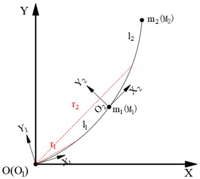
The study employs the 3-5-3 hybrid polynomial interpolation technique to address the challenge of trajectory planning for the manipulator's end effector traversing various path points. Figure 3 illustrates the segmented polynomial interpolation diagram associated with this approach.

Figure 3 Illustration of the 3-5-3 schematic diagram of interpolation function.

Any four known path points are selected in the motion trajectory for trajectory optimization design, which are noted as the start point S₁(0,θ₀), the path point S₂(t₁,θ₁), the path point S₃(t₂,θ₂), and the termination point S₄(t₃,θ₃), respectively. The trajectory is partitioned into three distinct segments by the specified path delineations, incorporating third-, fifth-, and third-degree polynomials successively.

• 1.

  Trajectory planning using cubic polynomials in the first stage (0 to t₁) is as follows:

  $$\begin{array}{}\text{(17)}& \left\{\begin{array}{l}{\mathit{\theta }}_{\mathrm{1}}\left(t\right)=a_{\mathrm{10}}+a_{\mathrm{11}}{t}_{\mathrm{1}}+a_{\mathrm{12}}{t}_{\mathrm{1}}^{\mathrm{2}}+a_{\mathrm{13}}{t}_{\mathrm{1}}^{\mathrm{3}},\\ {\dot{\mathit{\theta }}}_{\mathrm{1}}\left(t\right)=a_{\mathrm{11}}+\mathrm{2}{a}_{\mathrm{12}}{t}_{\mathrm{1}}+\mathrm{3}{a}_{\mathrm{13}}{t}_{\mathrm{1}}^{\mathrm{2}},\\ {\ddot{\mathit{\theta }}}_{\mathrm{1}}\left(t\right)=\mathrm{2}{a}_{\mathrm{12}}+\mathrm{6}{a}_{\mathrm{13}}{t}_{\mathrm{1}}.\end{array}\right.\end{array}$$
• 2.

  Within the second stage (t₁ to t₂), a fifth-degree polynomial is used for trajectory planning:

  $$\begin{array}{}\text{(18)}& \left\{\begin{array}{l}{\mathit{\theta }}_{\mathrm{2}}\left(t\right)=a_{\mathrm{20}}+a_{\mathrm{21}}{t}_{\mathrm{2}}+a_{\mathrm{22}}{t}_{\mathrm{2}}^{\mathrm{2}}+a_{\mathrm{23}}{t}_{\mathrm{2}}^{\mathrm{3}}+a_{\mathrm{24}}{t}_{\mathrm{2}}^{\mathrm{4}}+a_{\mathrm{25}}{t}_{\mathrm{2}}^{\mathrm{5}},\\ {\dot{\mathit{\theta }}}_{\mathrm{2}}=a_{\mathrm{21}}+\mathrm{2}{a}_{\mathrm{22}}{t}_{\mathrm{2}}+\mathrm{3}{a}_{\mathrm{23}}{t}_{\mathrm{2}}^{\mathrm{2}}+\mathrm{4}{a}_{\mathrm{24}}{t}_{\mathrm{2}}^{\mathrm{3}}+\mathrm{5}{a}_{\mathrm{25}}{t}_{\mathrm{2}}^{\mathrm{4}},\\ {\ddot{\mathit{\theta }}}_{\mathrm{2}}=\mathrm{2}{a}_{\mathrm{22}}+\mathrm{6}{a}_{\mathrm{23}}{t}_{\mathrm{2}}+\mathrm{12}{a}_{\mathrm{24}}{t}_{\mathrm{2}}^{\mathrm{2}}+\mathrm{20}{a}_{\mathrm{25}}{t}_{\mathrm{2}}^{\mathrm{3}}.\end{array}\right.\end{array}$$
• 3.

  Trajectory planning using cubic polynomials in the third stage (t₂ to t₃) is as follows:

  $$\begin{array}{}\text{(19)}& \left\{\begin{array}{l}{\mathit{\theta }}_{\mathrm{3}}\left(t\right)=a_{\mathrm{30}}+a_{\mathrm{31}}{t}_{\mathrm{3}}+a_{\mathrm{32}}{t}_{\mathrm{3}}^{\mathrm{2}}+a_{\mathrm{33}}{t}_{\mathrm{3}}^{\mathrm{3}},\\ {\dot{\mathit{\theta }}}_{\mathrm{3}}=a_{\mathrm{31}}+\mathrm{2}{a}_{\mathrm{32}}{t}_{\mathrm{3}}+\mathrm{3}{a}_{\mathrm{33}}{t}_{\mathrm{3}}^{\mathrm{2}},\\ {\ddot{\mathit{\theta }}}_{\mathrm{3}}=\mathrm{2}{a}_{\mathrm{32}}+\mathrm{6}{a}_{\mathrm{33}}{t}_{\mathrm{3}}.\end{array}\right.\end{array}$$

At the initiation point S₁ and the conclusion point S₄, assign zero values to their velocities and accelerations. The intermediate points S₂ and S₃ serve as connectors for the multi-segment interpolating polynomials, demanding consistent displacements, velocities, and accelerations at the boundary of these two points (Li, 2023).

The constraints are incorporated into Eqs. (17)–(19) and organized into matrix form as follows:

$$\begin{array}{}\text{(20)}& \mathbf{a}={\mathbf{A}}^{-\mathrm{1}}\mathit{\theta },\end{array}$$

where a represents the coefficient matrix, θ denotes the combination matrix of four path points, and A refers to the polynomial matrix with respect to time t.

3.2 Trajectory optimization based on MAPSO

The adaptive particle swarm optimization (APSO), as detailed by Zhang and Fu (2020), represents an optimization algorithm that leverages collective intelligence. Its fundamental concept involves emulating the social dynamics observed in bird flocks, facilitating efficient pursuit of optimal solutions through group-based collaborative search mechanisms.

The velocity and position formulation of the adaptive particle swarm optimization algorithm is as follows:

$$\begin{array}{}\text{(21)}& \left\{\begin{array}{l}\begin{array}{rl}{v}_{i,j}(t+\mathrm{1})& =\mathit{\omega }\cdot v_{i,j}\left(t\right)+c_{\mathrm{1}}{r}_{\mathrm{1}}\left|{\mathrm{pb}}_i\left(t\right)-x_{i,j}\left(t\right)\right|\\ & +c_{\mathrm{2}}{r}_{\mathrm{2}}\left|{\mathrm{gb}}_i\left(t\right)-x_{i,j}\left(t\right)\right|,\end{array}\\ x_{i,j}(t+\mathrm{1})=x_{i,j}\left(t\right)+v_{i,j}(t+\mathrm{1}).\end{array}\right.\end{array}$$

In this context, v_i,j(t) represents the velocity of the ith particle during the jth interpolation process after t iterations, while it also signifies the position reached by the ith particle during the same process. ω denotes the inertia weight; c₁ and c₂ are the individual and population learning factors, respectively; and r₁ and r₂ are random numbers within the interval [0,1]. pb_i(t) indicates the individual best value found by the ith particle during the current search process, whereas gb_i(t) represents the global best value discovered by all particles in the same process.

However, the inertia weight, as well as the individual and population factors in the APSO algorithm, is a fixed value. This rigidity can lead to issues such as falling into local optima and a lack of adaptability to the search environment. To address these limitations, this paper proposes an enhancement to the APSO algorithm by optimizing the three parameters: inertia weight (ω), individual learning factor (c₁), and population learning factor (c₂). This results in the development of the MAPSO algorithm, which aims to improve the algorithm's flexibility and effectiveness in navigating the solution space.

3.2.1 Inertia weight (ω)

Transformation of constant inertia weights into nonlinear inertia weight functions using segmented tangent function:

$$\begin{array}{}\text{(22)}& \left\{\begin{array}{l}\mathit{\omega }=\left({\mathit{\omega }}_{max}-{\mathit{\omega }}_{min}\right)\cdot \tan \left(\mathrm{0.875}{\left(\mathrm{1}-\frac{\text{iter}}{{\text{iter}}_{max}}\right)}^k\right)+{\mathit{\omega }}_{min},\\ \text{iter}<\mathrm{0.6}\cdot {\text{iter}}_{max},\\ \mathit{\omega }=\mathrm{0.2}+\mathrm{0.1}\cdot \text{rand}\left(\right),\\ \text{iter}>\mathrm{0.6}\cdot {\text{iter}}_{max},\end{array}\right.\end{array}$$

where ω_max is the maximum value of inertia weight, taking the empirical value of 0.9. ω_min is the minimum value of inertia weight, taking the empirical value of 0.2. iter_max is the number of iterations, and k is the control factor (generally taking 0.6).

3.2.2 Individual learning factor (c₁) and group learning factor (c₂)

A trigonometric function is used for dynamic adaptive adjustment, which closely combines the values of the two learning factors with the current iteration times of the particle. The function's representation is detailed as follows:

$$\begin{array}{}\text{(23)}& \left\{\begin{array}{l}{c}_{\mathrm{1}}=c_{max}-\left(c_{max}-c_{min}\right)\cdot {\sin }^{\mathrm{2}}(\frac{\mathit{\pi }}{\mathrm{2}}\cdot \frac{\text{iter}}{v_{max}}),\\ c_{\mathrm{2}}=c_{min}+\left(c_{max}-c_{min}\right)\cdot {\sin }^{\mathrm{2}}(\frac{\mathit{\pi }}{\mathrm{2}}\cdot \frac{\text{iter}}{{\text{iter}}_{max}}).\end{array}\right.\end{array}$$

The optimization of the interpolation time for the 3-5-3 hybrid polynomial is achieved through the application of the MAPSO algorithm. Subsequently, the total time consumed by each joint, denoted as t₁, t₂, and t₃, in executing the three-segment interpolation trajectory is aggregated to derive the fitness function for an individual joint. This fitness function is mathematically expressed as follows:

$$\begin{array}{}\text{(24)}& \text{min}f=T=\sum _{t_{\mathrm{0}}}^{t_f}t=\sum _{i=\mathrm{0}}^{\mathrm{1}}\left(t_{i+\mathrm{1}}-t_i\right).\end{array}$$

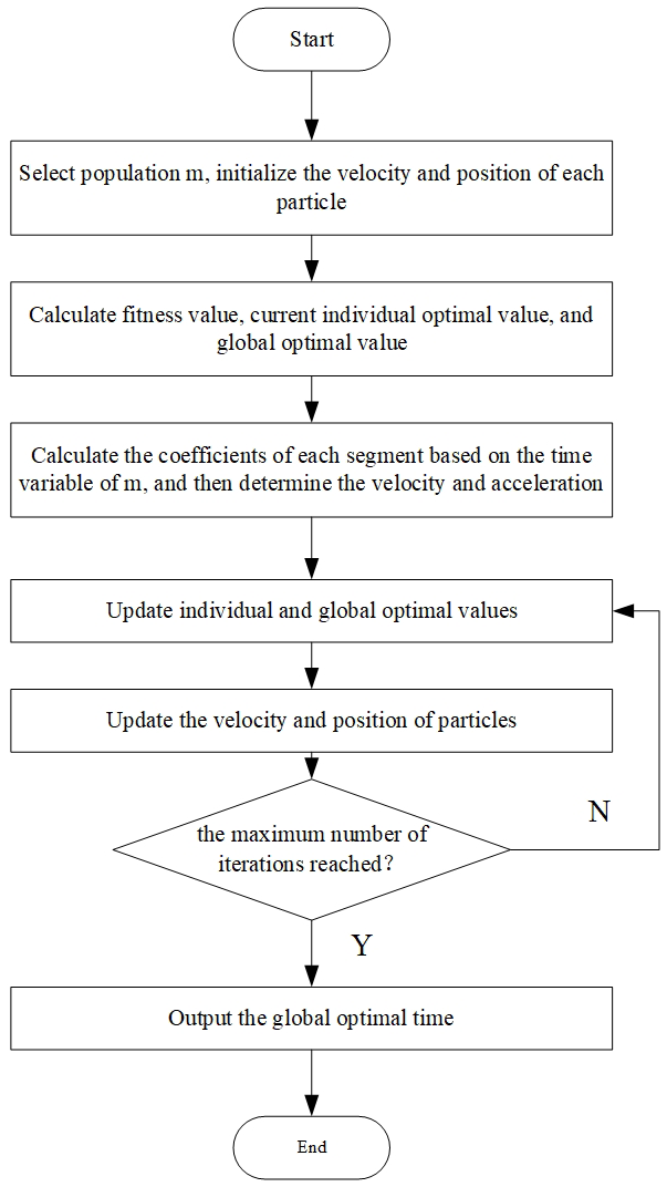
3.2.3 Process of MAPSO

The precise procedures of the enhanced optimization algorithm are illustrated in Fig. 4.

• 1.

  Define the scope of particle attributes such as positions and velocities, the population magnitude denoted as m and the upper limit of iterations and establish the initial positions and velocities for each particle within the populace.

• 2.

  Log the most extreme values and present positions of the individual optimal and global optimal entities.

• 3.

  Utilize the N 3D temporal vectors derived from the initialization in Eq. (20) to determine the coefficients for each segmenting function. Subsequently, apply them to Eqs. (17) to (19) to compute the three-segment motion path, velocity, and acceleration for each articulation.

• 4.

  Determine the compliance of the velocity and acceleration exhibited by the three-segment trajectories pertaining to every joint of the robotic arm with the prescribed kinematic limitations. Should all three-segment trajectories adhere to the stipulated constraints, incorporate the duration of the three-segment trajectories into Eq. (24) for the computation of the fitness metric while documenting the prevailing positional data. Conversely, should the velocity or acceleration of any of the three-segment trajectories surpass the established constraints, assign a significantly elevated fitness value to the current particle to guarantee its exclusion during subsequent iterations.

• 5.

  Update the weight ω and learning factors c₁ and c₂ according to Eqs. (22) and (23), and incorporate them into the initial APSO equations to adjust the positions and velocities of the particles.

• 6.

  The sub-iteration loop is executed by assessing the fitness values of the individual pole and the global pole from which the particle exhibiting the highest fitness is chosen, representing the optimal pole.

• 7.

  If the termination criterion is not met, step 3 will be initiated, and the iteration will cease once the termination criterion is fulfilled.

Figure 4 The process of the improved adaptive particle swarm optimization algorithm.

3.3 Simulation analysis

The origin of the coordinate system was established at the joint motor 1, which controlled the flexible link L₁. Initially, both flexible rods were aligned parallel to the ground. Four specific path points within the reachable space of the two flexible links were identified and are detailed in Table 2.

Table 2 The target trajectory point parameter information of the flexible manipulator.

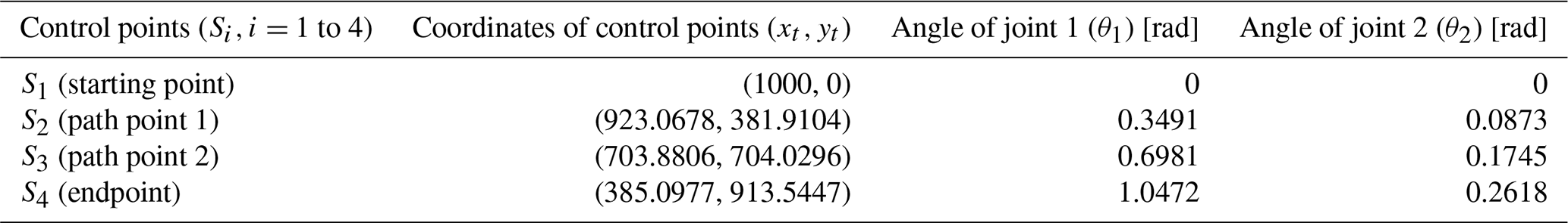
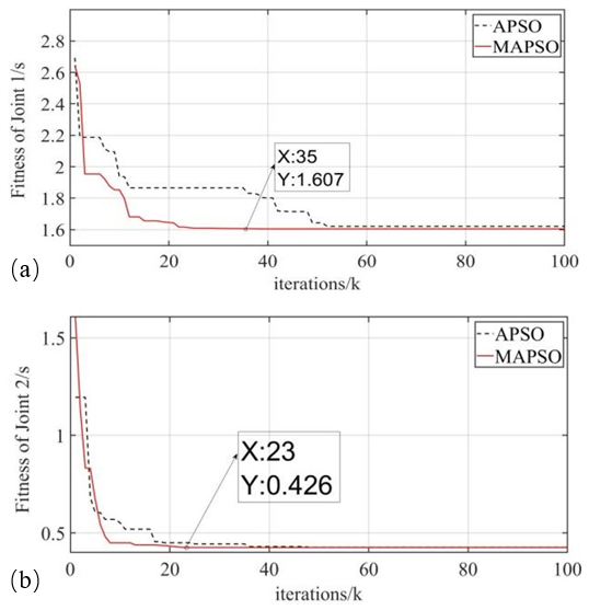
The initial total duration was established to be 6 s, with individual intervals of 2 s each. Utilizing MATLAB, a simulation was conducted to determine the convergence count and time for both the standard APSO algorithm and the novel MAPSO algorithm detailed in this study, as illustrated in Fig. 5.

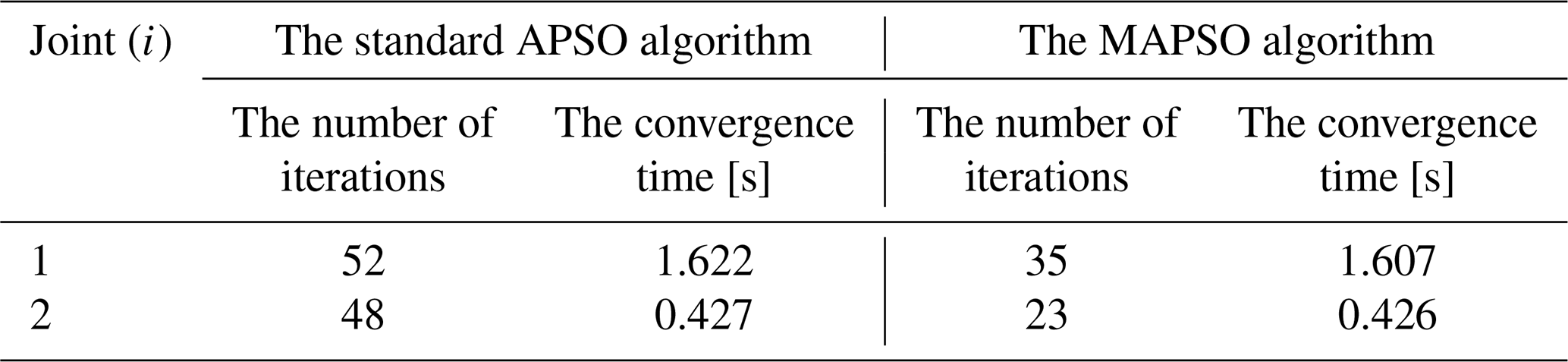
As shown in Fig. 5, comparing to the standard APSO algorithm, when the MAPSO algorithm optimized the target trajectories of the two flexible arms, the number of iterations of joint 1 decreased from 52 to 35, while the number of iterations of joint 2 decreased from 48 to 23. Meanwhile, the convergence time of the MAPSO algorithm was also better than that of the standard APSO algorithm. The specific comparison results regarding the number of global convergences and convergence times are presented in Table 3.

Figure 5 Process of convergence of joints: (a) joint 1 and (b) joint 2.

Table 3 Comparative analysis of two algorithms.

The time taken for each trajectory segment optimized by the MAPSO algorithm had been compared with the time required by the conventional setting method, as presented in Table 4.

Table 4 Comparative table of time spent on each trajectory segment.

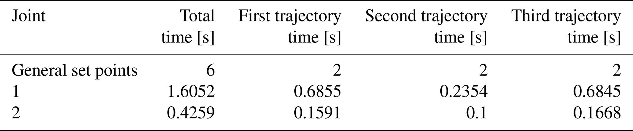
As indicated in Table 4, the maximum values of the two joints for each segment trajectory were considered the overall running time for that segment: t₁ = 0.6855 s, t₂ = 0.2354 s, and t₃ = 0.6845 s. Consequently, the total running time of the robotic arm, t, was calculated to be 1.6054 s. This represented a reduction of 4.3946 s compared to the pre-optimization 3-5-3 segmented polynomial trajectory planning.

The variation curves of angular displacement, angular velocity, and angular acceleration for the action of interpolating polynomials optimized by the MAPSO algorithm are illustrated in Fig. 6.

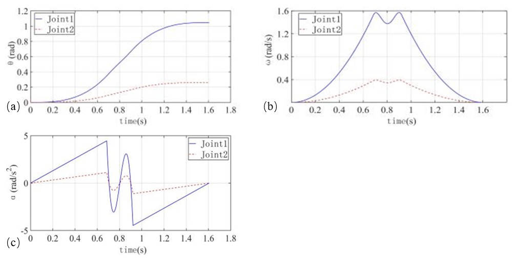
Figure 6 Improved algorithm 3-5-3 joint variation parameters under the action of hybrid polynomial interpolation. (a) Angular displacement, (b) angular velocity and (c) angular acceleration.

The simulation results demonstrated that the two joints of the flexible manipulator can accurately navigate through each path point when driven by the MAPSO algorithm. Additionally, the velocities and accelerations of the joints adhered to the specified boundary constraints while achieving a time-optimal path. However, it is noteworthy that the values of the joints' velocities and accelerations were relatively high. Specifically, the maximum velocity for joint 1 was 1.56 rad s⁻¹, while for joint 2, it was 0.393 rad s⁻¹. The maximum accelerations recorded were 4.458 rad s⁻² for joint 1 and 1.110 rad s⁻² for joint 2. The graph clearly illustrates significant fluctuations during the intermediate stages, characterized by sharp changes in acceleration, which are attributed to the optimization of the MAPSO algorithm based on runtime.

4 Trajectory tracking strategy based on MAPSO-FuzzyPD

The studies indicated that while the MAPSO algorithm facilitates quicker attainment of target positions for the manipulator, it simultaneously elevated the speed and acceleration during operation, leading to increased vibrations. Consequently, it was essential to investigate vibration suppression techniques in trajectory tracking to mitigate the adverse effects of these vibrations on the robotic arm system. Implementing effective vibration control strategies will enhance the overall stability and performance of the manipulator, ensuring smoother operation and improved accuracy in task execution.

After trajectory planning, it is essential to employ algorithms and other methods to ensure that the robotic arm accurately follows the intended path (Chen et al., 2022). To address the inaccuracies in the dynamics model and reduce jitter in the tracking system, this paper proposed a MAPSO-FuzzyPD controller. This controller was designed with robustness to counteract the uncertainties affecting joint trajectory tracking control. By integrating the MAPSO algorithm with a Fuzzy-PD control strategy, the proposed approach aimed to enhance the tracking performance of each joint in the manipulator, ensuring smoother and more precise execution of the planned trajectory.

4.1 Fitting of joint angular displacements

The input for the trajectory tracking control consists of the joint angular displacements calculated in Sect. 3. To enhance the accuracy, smoothness, and stability of the controller's output as well as to prevent potential issues during the solution process, the angular displacement curve is further refined.

A higher-order polynomial function was used to fit and optimize the angular displacements of the two joints, and the joint path points in Table 2 were added as constraints to obtain a smoother target trajectory curve. The errors in the fitted curves of angular displacements of the two joints with the original 3-5-3 interpolation are shown in Fig. 7.

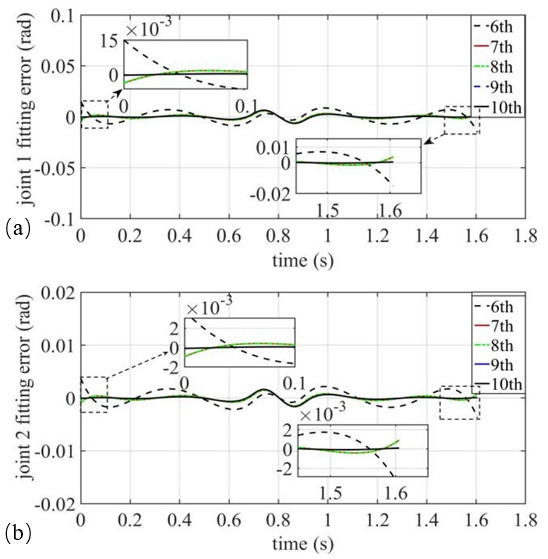
Figure 7 Fitting error in the nth-order polynomial fitted to the angular displacements of the two joints: (a) joint 1 and (b) joint 2.

Given that polynomials of a degree higher than nine were susceptible to overfitting, the analysis indicated that seventh- and eighth-degree polynomials yield smaller fitting errors. Additionally, the 3-5-3 mixed polynomials exhibit odd function properties, which may not be ideal for this application. Therefore, this paper selected the fitting curve of the seventh-degree polynomial as the final target curve. This choice balanced complexity and accuracy, ensuring a smooth trajectory while minimizing the risk of overfitting.

4.2 Fuzzy PD-based trajectory tracking controller

The integral component of PID control serves to eliminate steady-state error. However, it can also amplify noise and interference within the system. This amplification often leads to slow response times and unstable outputs, which can cause noticeable jitter in the operation of flexible robotic arms. To address these issues, this paper employed a fuzzy PD controller for trajectory tracking control. The fuzzy PD controller not only compensates for errors in trajectory tracking but also enhances control accuracy and increases the robustness of the system. The control block diagram for the fuzzy PD controller is illustrated in Fig. 8, demonstrating its application in improving trajectory tracking performance.

Figure 8 Fuzzy PD control block diagram.

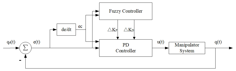
In Fig. 8, e(t) is the joint angle following error, e_c(t) is the rate of change in the following error of the joint angle, and ΔK_P and ΔK_D are the supplementary parameters corrected by the fuzzy controller. At this time, the fuzzy PD controller has two inputs, e and e_c, and two outputs, ΔK_P and ΔK_D. ΔK_P and ΔK_D are corrected by the fuzzy controller in real time by the action of the fuzzy rules, and the outputs are connected and externalized to the PD controller, which is combined with the given initial values of the PD parameters, K_P0 and K_D0, and then finally applied to the robotic arm system. The fuzzy PD parameter self-tuning controller expression is obtained as follows:

$$\begin{array}{}\text{(25)}& \left\{\begin{array}{l}{K}_P=K_{P\mathrm{0}}+\mathrm{\Delta }{K}_P,\\ K_D=K_{D\mathrm{0}}+\mathrm{\Delta }{K}_D.\end{array}\right.\end{array}$$

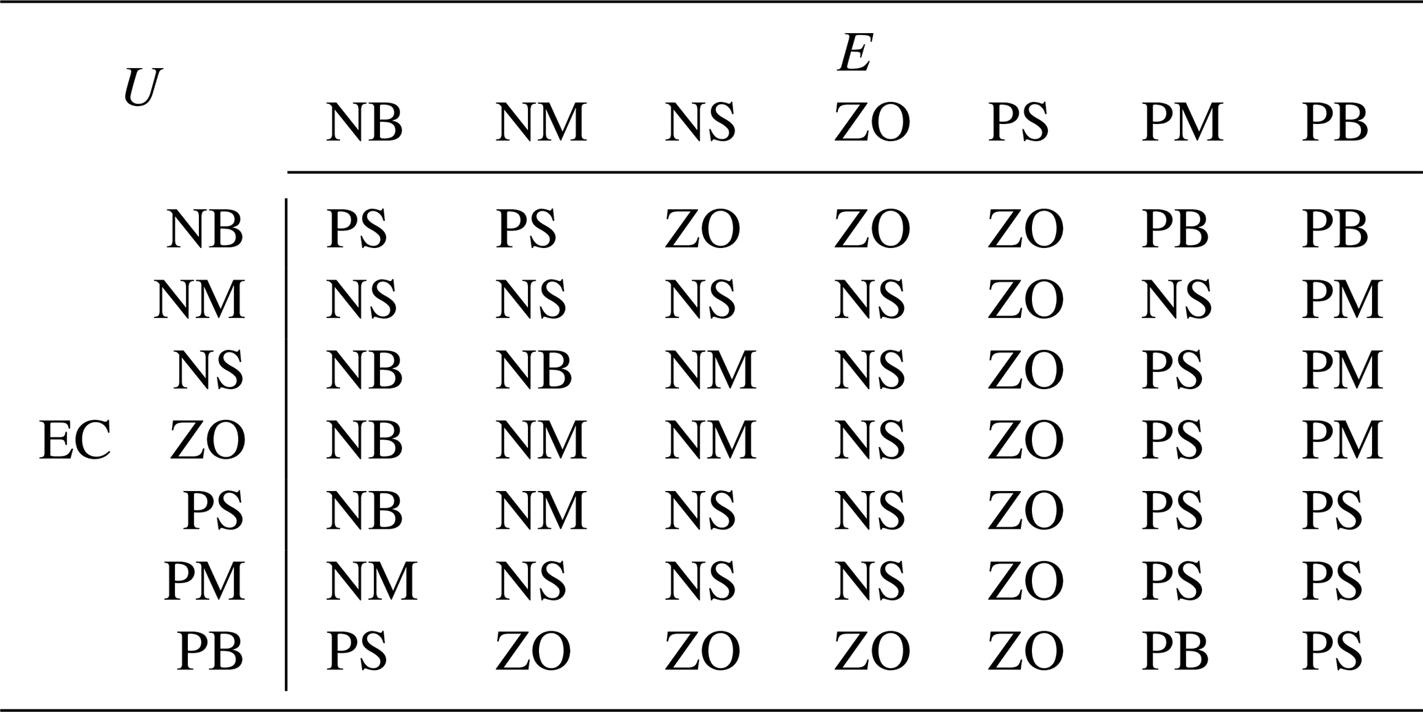
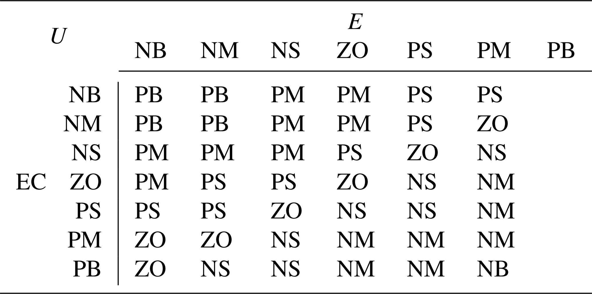
In this study, the triangular membership function was selected for the fuzzy control solution. Drawing from PD parameter tuning experiences and manual testing, the input variable domains for e and e_c were defined to be within $[-\mathrm{0.5},\mathrm{0.5}]$, while the output variable domains for ΔK_P and ΔK_D were set to $[-\mathrm{15},\mathrm{15}]$. The triangular membership function employs the center of gravity method, resulting in seven fuzzy sets: negative large (NB), negative medium (NM), negative small (NS), zero (ZO), positive small (PS), positive medium (PM), and positive large (PB). Based on expert knowledge and relevant literature regarding the regulation of these variables, as well as the fundamental principles of control quantity adjustment, the fuzzy rules governing the control of ΔK_P and ΔK_D parameters have been compiled and are presented in Tables 5 and 6. These rules facilitate effective tuning of the fuzzy PD controller, ensuring improved trajectory tracking performance.

Table 5 The fuzzy rule control table of ΔK_P.

Table 6 The fuzzy rule control table of ΔK_D.

4.3 MAPSO-based fuzzy PD trajectory tracking controller

While the fuzzy controller effectively adjusts the parameters of the PD controller, the initial parameters K_P0 and K_D0 must still be determined manually through experiments, which can lack rigor. To address this, this paper employed an improved adaptive particle swarm optimization (MAPSO) algorithm, known for its straightforward principles, strong learning capabilities, and ease of convergence. The proposed approach combined the MAPSO algorithm with fuzzy PD control to formulate a MAPSO-FuzzyPD controller. This design first optimized the initial values of the proportional and derivative parameters, followed by fine-tuning these values using the fuzzy controller. This combination enhanced the overall control performance and robustness of the system. The improved schematic block diagram illustrating this methodology is presented in Fig. 9.

Figure 9 Block diagram of MAPSO-based fuzzy PD controller structure.

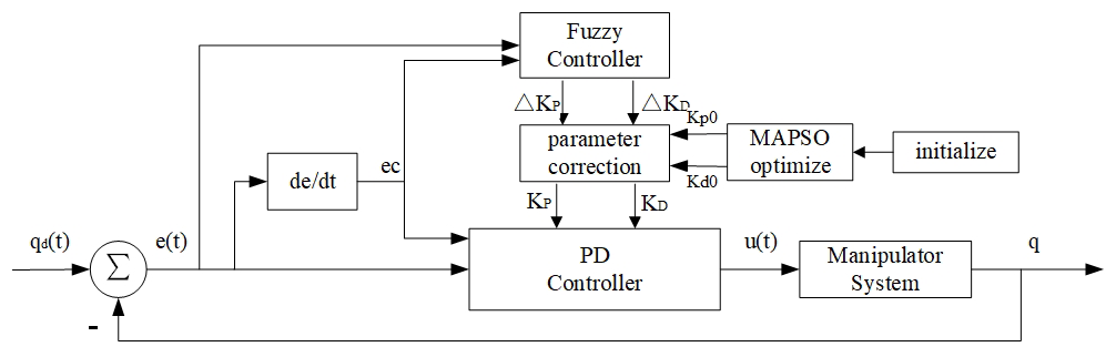
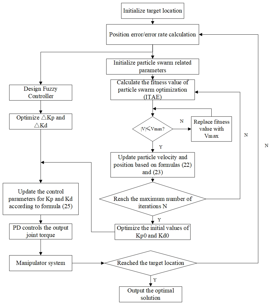
The optimized process of the improved adaptive particle swarm optimization algorithm discussed in Sect. 3.2.3, along with the modified structure diagram of the fuzzy PD controller, is illustrated in Fig. 10 for the fuzzy PD control system based on MAPSO.

Figure 10 The fuzzy PD control system based on MAPSO.

The simulation model built using Simulink is shown in Fig. 11.

Figure 11 Simulink simulation model.

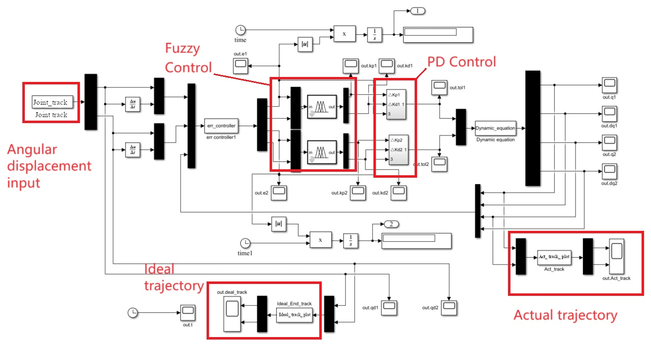
4.4 Simulation analysis of MAPSO-FuzzyPD controller

To validate the effectiveness of the control strategy proposed in this paper, a numerical simulation analysis was conducted. The population size (N) was set to 30, the maximum number of iterations (iter_max) was 100, and the dimension count was 4. representing the proportional control of two joints, along with the initial values of differential parameters, which were bounded within a range of $\pm [\mathrm{200},\mathrm{200},\mathrm{125},\mathrm{125}]$. The initial calculation of proportional and differential values was performed using the MAPSO algorithm, with corresponding code written for continuous iteration to obtain the optimal values based on the fitness function. These optimal values were then stored in the MATLAB workspace. Simulation was conducted using the trajectory tracking controller established in Fig. 11. During the trajectory tracking process, the PD control section automatically retrieved the optimal initial values of K_P0 and K_D0 from the workspace, incorporating fuzzy control for real-time adjustments. The results of the simulation, specifically the error between the theoretical and actual tracking angles of the two joints, are illustrated in Fig. 12.

The illustration in Fig. 12 demonstrates that the enhanced fuzzy PD controller exhibits superior performance in real-time tracking of joints 1 and 2 when contrasted with both the PD and the fuzzy PD controllers. Notably, it effectively aligns the joint trajectories with the desired targets, eliminating initial oscillations observed during trajectory tracking.

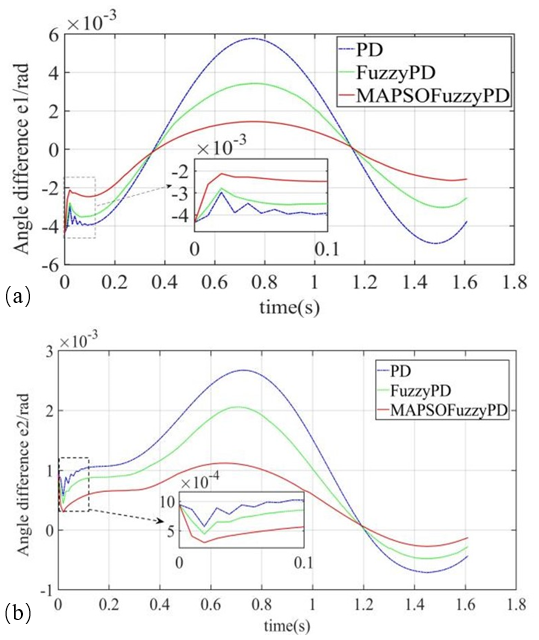
Figure 12 Angular difference from ideal trajectory with three control strategies: (a) joint 1 and (b) joint 2.

The angular velocity tracking and control torque curves for the three control strategies are shown in Fig. 13.

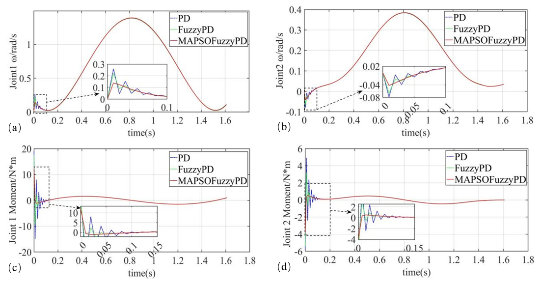
Figure 13 Angular velocity tracking and control torque curves. (a) Angle tracking velocity of joint 1. (b) Angle tracking velocity of joint 2. (c) Control torque of joint 1. (d) Control torque of joint 2.

As shown in Fig. 13, the improved Fuzzy PD controller effectively eliminated velocity and moment oscillations during the initial phase compared to previous control strategies. Specifically, the MAPSO-FuzzyPD controller reduced the maximum tracking velocity for joint 1 from 0.22 to 0.14 rad s⁻¹, with the duration of this peak velocity being shortened to just 0.01 s. For joint 2, the maximum tracking velocity decreased from 0.067 to 0.04 rad s⁻¹, also with a duration reduction to 0.01 s. Regarding torque, the variation range of the starting torque for joint 1 was significantly improved, now fluctuating between −1.1 and 12.4 N m. This represented a reduction of 61.3 % compared to the maximum starting torque observed with the PD controller and a 40.3 % decrease compared to the fuzzy PD controller. For joint 2, the starting torque variation was reduced to between −3.8 and 0.52 N m, which was 57.9 % less than the maximum starting torque of the PD controller and 42.1 % less than that of the fuzzy PD controller. These results highlighted the enhanced stability and performance of the MAPSO-FuzzyPD controller during the onset phase, leading to smoother operation with reduced oscillations.

The simulation results clearly demonstrated the superiority of the MAPSO-FuzzyPD control strategy.

5 Experimentation and analysis

The physical platform of the 2-degree-of-freedom flexible manipulator built in this paper was mainly composed of three parts: mechanical system, electrical system, and control system, as shown in Fig. 14. The electrical system comprised several key components: articulated motor 1 (HT8115-J9), articulated motor 2 (HT8108-J9), a motor power supply, and an acceleration sensor (Weite Intelligent six-axis accelerometer gyroscope WT61C-TTL). The control system consisted of a PC host and an STM32 control board, which work together to manage and execute the control algorithms. This setup allowed for precise coordination of the motors and monitoring of system performance through the acceleration sensor, enabling effective control and feedback mechanisms essential for optimal operation.

Figure 14 Experimental platform.

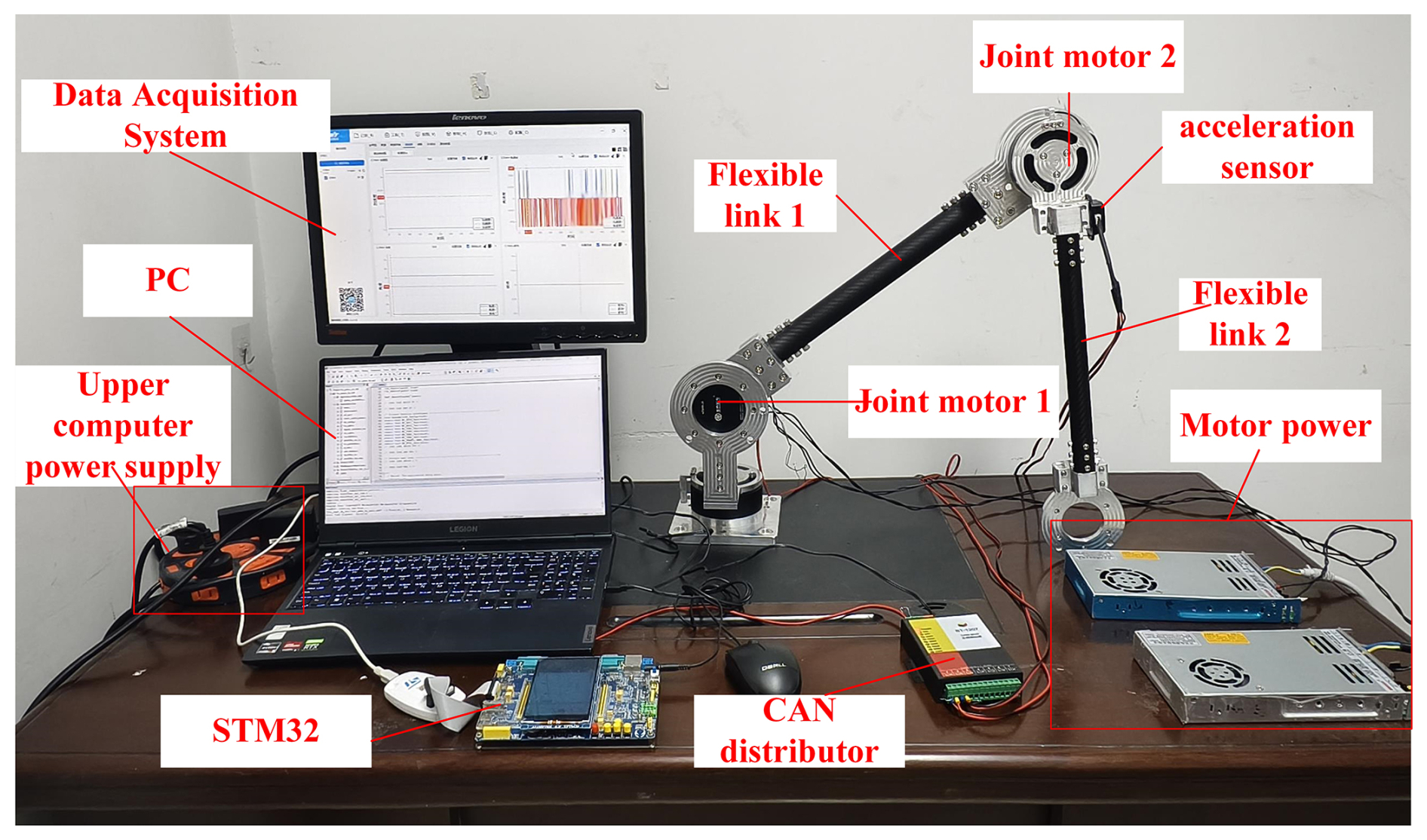
The control strategy involved developing a control program for the articulated motors using MDK5. This program was then uploaded to the STM32 control board via an ST-LINK, facilitating communication between the PC host and the lower computer. Once the commands were received, the STM32 control board parsed them and executed the necessary arithmetic operations using its internal processor. Based on these calculations, it determined the appropriate control signals for each joint motor. These control signals were subsequently transmitted to the respective joint motors through the controller area network (CAN) bus, ensuring precise and coordinated movement of the articulated system. This setup allowed for real-time control and adjustment, enhancing the overall responsiveness and performance of the system.

The experiment employed the optimized multi-path joint angle function from Sect. 4.1 as the target trajectory for the motor joint angles. The motor control program was integrated to enable the motor-controlled manipulator to follow four specified target paths, as detailed in Table 2. This movement was executed under three different control strategies: PD control, fuzzy PD control, and MAPSO-FuzzyPD control. The primary goals of the experiment were to assess the trajectory tracking performance of joint 1 and joint 2 and to evaluate the vibration characteristics at the end of flexible arm 2, specifically at the end effector.

The total duration of the experiment was 1.61 s, with a data collection precision set at 0.01 s. The data acquisition system extracted real-time data from various positions and exported them to a spreadsheet for subsequent data fitting using MATLAB. And the angular trajectory following curve and the vibration curve at the end of the flexible manipulator is as shown in Figs. 15 and 16, respectively.

Figure 15 Joint angles under various control strategies: (a) joint 1 and (b) joint 2.

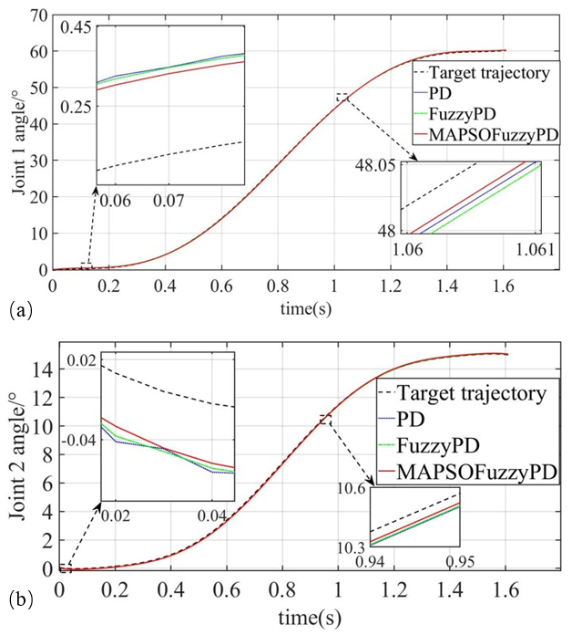
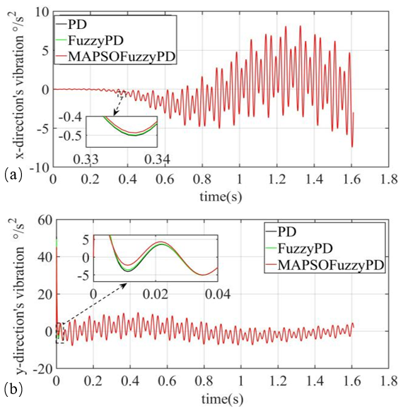
Figure 16 Vibration at the end of the manipulator. (a) Vibration of the end in the x direction. (b) Vibration of the end in the y direction.

In Fig. 15, the overall trend indicated that under the influence of the three control strategies, the motors driving joints 1 and 2 were able to closely track the target trajectory in real time, maintaining smooth operation within an acceptable error range. However, during the trajectory tracking phase, it was observed that both PD control and fuzzy PD control exhibit a greater deviation from the target trajectory compared to the MAPSO-FuzzyPD control. This suggested that the MAPSO-FuzzyPD control provided better accuracy in trajectory tracking, resulting in reduced error and enhanced performance of the flexible manipulator throughout the experiment. Moreover, the results indicated that, compared to the desired trajectory, all three methods exhibit a degree of lag due to uncertainties such as friction and aerodynamic damping present in the physical model during motion. Additionally, the flexibility and large length-to-diameter ratio of the flexible manipulator contribute to this lag, potentially leading to deviations in end-effector positioning. Future studies could focus on optimizing performance by integrating vibration control techniques.

Figure 16 shows the real-time variation curves of the vibration acceleration components at the end of the manipulator under the three control actions, and the end vibration situations were very close to each other due to the small error between the actual tracking trajectories of the three controllers. During the initial phase (0 to 0.4 s), the vibration acceleration amplitude at the end of the arm in the x direction for all three control strategies was nearly zero, indicating the successful implementation of a “soft start” in this direction. In contrast, in the y direction, the effects of gravity lead to a brief blocking torque during the instantaneous start, resulting in a significant amplitude of vibration at the arm's end. However, all three controllers managed to return the end of the arm to smooth tracking within 0.02 s, with the MAPSO-FuzzyPD control demonstrating slightly lower acceleration amplitudes compared to the other two controllers. From 0.4 to 1.61 s, the tracking speeds of the three control strategies showed minimal differences, leading to similar vibration levels at the end of the flexible arm during this period. As the joints approached the target position, the vibration acceleration diminished due to the gradual reduction in speed. After 1.61 s, once the two joints reached their target positions smoothly, the absence of active and passive vibration suppression strategies at the end of the arm results in residual vibrations of the flexible arm, highlighting an area for further investigation in future studies.

Based on the experimental results, both joints exhibit smooth trajectory tracking with minimal deviation. Notably, the MAPSO-FuzzyPD controller outperforms the other two control methods in terms of both trajectory tracking accuracy and vibration control. This demonstrates the effectiveness and advantages of the proposed control strategy in this paper, highlighting its potential for improved performance in robotic applications. The findings suggest that the MAPSO-FuzzyPD controller could be a valuable approach for enhancing the stability and responsiveness of robotic systems in dynamic environments.

6 Conclusions

In this paper, the 2-degree-of-freedom flexible manipulator was examined as the primary research object, focusing on three key aspects: dynamics modeling, trajectory planning, and trajectory tracking. The main conclusions drawn from this study are as follows:

• 1.

  The flexural deformation of the pliable manipulator was elucidated through the utilization of the assumed modal approach, and the dynamic equations governing the 2-degree-of-freedom manipulator were formulated through the amalgamation of the Lagrangian method.

• 2.

  Aiming at the problems of solving the coefficients of 3-5-3 interpolating polynomials and the difficulty of selecting the optimal value, the adaptive particle swarm optimization algorithm was improved by a nonlinear segmented tangent inertia weight function and dynamically adjusting the learning factor based on a trigonometric function. A 3-5-3 hybrid polynomial algorithm based on MAPSO was proposed, and simulation experiments were carried out on the basic trajectory with time as the optimization objective. Simulation results indicated that both joints of the flexible manipulator accurately traversed each path point under the proposed algorithm. The resulting position, velocity, and acceleration profiles were smooth, continuous, and free of abrupt changes, thereby satisfying the specified boundary constraints.

• 3.

  A trajectory tracking controller based on MAPSO-FuzzyPD was constructed by modifying the fuzzy PD controller with the MAPSO algorithm and analyzed by simulation experiments. The outcomes of the simulation reveal notable improvements when comparing FuzzyPD with respect to tracking speed and torque control. Specifically, the maximum tracking speed of joint 1 decreased from 0.22 to 0.14 rad s⁻¹, with a reduced duration of 0.01 s. Similarly, the maximum tracking speed of joint 2 decreased from 0.067 to 0.04 rad s⁻¹, also with a duration reduction to 0.01 s. Consequently, the efficacy in determining the optimal PD control parameter initial value was significantly enhanced. In terms of torque, the range of starting torque for joint 1 decreased to −1.1 and 12.4 N m, representing a 61.3 % and 40.3 % decrease compared to the maximum starting torque of PD control and FuzzyPD, respectively. Likewise, the starting torque range for joint 2 decreased to −3.8 and 0.52 N m, indicating a 57.9 % and 42.1 % decrease compared to the maximum starting torque of PD control and FuzzyPD, respectively. These results demonstrated the algorithm's effectiveness in mitigating the initial vibrational phenomena observed in tracking angular displacement, angular velocity, and torque, thereby facilitating smoother motor and robotic arm control operations.

Finally, an experimental platform for the flexible manipulator was established, and the experimental results further validated the effectiveness and feasibility of the algorithm proposed in this paper concerning joint trajectory tracking.