the Creative Commons Attribution 4.0 License.
the Creative Commons Attribution 4.0 License.
 | 20 Jun 2024
High-precision velocity control of direct-drive systems based on friction compensation
Baoyu Li
Xin Xie
Bin Yu
Yuwen Liao
Dapeng Fan
Friction is a complex nonlinear behavior and a significant factor that limits the performance improvement of servo systems. Drawing inspiration from the particular prestiction friction phenomenon exhibited by direct-drive systems upon sudden emergency stops, this paper introduces a dynamic and continuous friction model that includes pre-sliding and gross-sliding regimes. By analyzing the friction dynamics when the system velocity briefly reaches zero, a concave function related to the previous state of the system is used to describe the transition of friction in the pre-sliding regime. The Stribeck model is employed to represent the friction behavior in the gross-sliding regime, ensuring stationarity during friction regime switching. Based on the established friction model, a friction compensation method is developed in velocity control mode. The superior performance of this proposed friction compensation method is confirmed through sine-tracking experiments. Compared with the proportional integral controller and the Stribeck friction compensation method, the peak-to-peak value of the proposed method is reduced by up to 61.1 %, and the root-mean-square (rms) value is reduced by up to 81 %, with the smallest rms value reaching 0.13 mrad, significantly improving the dynamic tracking performance of the system.
- Article
(2155 KB) - Full-text XML
- BibTeX
- EndNote


Friction is a complex, nonlinear phenomenon, and its behavior is influenced by various factors, including the relative velocity and position of the contacting surfaces, material properties, lubrication, and temperature. Due to the complexity of the influencing factors, there are significant differences in friction characteristics, which makes it difficult to provide an accurate description of friction behavior. In applications such as electro-optical targeting systems and high-precision stable platforms, friction can introduce discontinuities and nonlinearities near low and zero velocities, leading to dead zones and creeping phenomena that severely impact the velocity-tracking accuracy of the system. In order to overcome the influence of friction on the control accuracy of the system, current research focuses on how to accurately describe the friction transition behavior of the system in the very low-velocity stage and design a compensation scheme based on a friction model to reduce or eliminate the influence of friction (Yin et al., 2023).
In the study of friction behavior characterization, numerous scholars have proposed various friction models through observations of frictional phenomena (Marton and Lantos, 2007). As research on friction has deepened, the friction model has undergone a transition from static to dynamic models (Marques et al., 2016; Pennestrì et al., 2016). Among these, the more practical friction models include the Stribeck model (Makkar et al., 2005) and the LuGre model (Li et al., 2017; Marques et al., 2021). In the static friction model represented by the Stribeck model, there is uncertainty in describing friction at zero velocity. In practical applications, due to the influence of velocity measurement noise, friction often fluctuates between forward and reverse static friction, which is seriously inconsistent with the friction in the actual system. For this reason, Feng et al. (2019) introduced the Karnopp theory into the Stribeck model when establishing an electro-hydraulic system. They proposed the concept of a zero-velocity threshold and expressed the friction within this threshold as a straight line. Wang et al. (2023) introduced the concept of cascading the Stribeck model with a first-order low-pass filter, aiming to mitigate the abrupt changes in friction that occur when the velocity passes zero. Liu et al. (2023) employed the hyperbolic tangent function with varying coefficients to approximate the Stribeck model, offering an alternative representation. Furthermore, Wan et al. (2022), Yao et al. (2015), Wu et al. (2014), Márton et al. (2009), and Thenozhi et al. (2022) addressed the discontinuity issues inherent in the Stribeck model by modifying its structure. Their goal is to develop a smooth and continuously distinguishable friction model, eliminate the influence of friction through friction compensation, and improve control accuracy.
The LuGre model, based on the Stribeck model, improves the discontinuity of friction at zero velocity by introducing a nonlinear differential equation (Marques et al., 2021). This enhancement enables the LuGre model to not only describe friction behavior at exceedingly low velocities, but also to capture nuanced characteristics such as sticky-slip oscillations and zero-slip displacement (Huang et al., 2019). These capabilities lay a foundation for comprehensively describing and analyzing the microscopic state of friction, ultimately enabling the effective suppression of friction. Therefore, scholars have developed high-precision compensation methods using the LuGre model in various application fields, including the two-axis optoelectronic stabilized platform (Hu et al., 2023), electro-hydraulic servo system (Feng et al., 2022), wheeled planetary rover (Yu et al., 2022), dual-drive hydraulic lead screw micro–nano feed system (Liu et al., 2022), and permanent-magnet synchronous motor (Zhang et al., 2022). These methods have achieved excellent results. However, in the gross-sliding regime of friction, the LuGre model exhibits the same behavior as the Stribeck model and is still influenced by velocity measurement noise. In the stage of extremely low velocity, near zero velocity, there will still be instability in the friction torque. To better describe the friction behavior in the low-velocity stage, Bazaei and Moallem (2009) divided the friction model into three phases, the stiction phase, kinetic phase, and prestiction phase, and the friction phase is determined by identifying that the velocity decreases to a certain desired velocity and duration. Similarly, to describe friction within the zero-velocity threshold, a two-state dynamic friction model (Ruderman and Bertram, 2013; Ruderman, 2014) is proposed, and this model includes the pre-sliding and sliding stages of friction. However, the above model is limited by the resolution of the velocity sensor, and the velocity threshold is set at more than 2° s−1, which fails to accurately describe friction behavior at extremely low velocities from a more microscopic perspective.
Due to the strong correlation between friction and the motion state prior to the system velocity briefly reaching zero, the current friction models that have been proposed are unable to accurately describe this microscopic characteristic of friction. This article introduces a dynamic continuous friction model composed of the pre-sliding and gross-sliding regimes, and this model is based on the particular prestiction friction phenomenon observed in the direct-drive system (DDS) after a sudden emergency stop. The main highlight of this model lies in its utilization of both the current and previous states of the system to effectively describe the friction behavior at zero velocity, thereby achieving a more precise description of friction. Building upon this friction model, a friction compensation method for the DDS is constructed within the velocity control mode, and the primary objective of this method is to achieve precise friction compensation and high-precision velocity control for the system.
In the current closed-loop mode of the DDS, the system is excited to move with a current ramp signal, the input signal is set to zero when the output angle of the system reaches a given threshold, and the angular position response is recorded to characterize the acceleration and free deceleration processes of the system. The angular position response is closely related to the state of the system prior to this test, and the system exhibits the particular prestiction friction phenomenon.
The angular position response of the DDS is shown in Fig. 1. When the system is subjected to a sudden emergency stop and the above test is conducted in the same direction as before the emergency stop, the acceleration process slows down and the output angle of the system crosses the starting point during the free deceleration process, showing a “reverse overshoot” phenomenon marked as “Same direction” in the figure and simplified as “sd” in the legend. When the above test is conducted in the opposite direction to that before the emergency stop, the acceleration process becomes faster and the output angle of the system fails to return to the starting point during free deceleration, which is marked as “Opposite direction” in the figure and simplified as “od” in the legend. The angle thresholds for the different curves are also given in the legend.
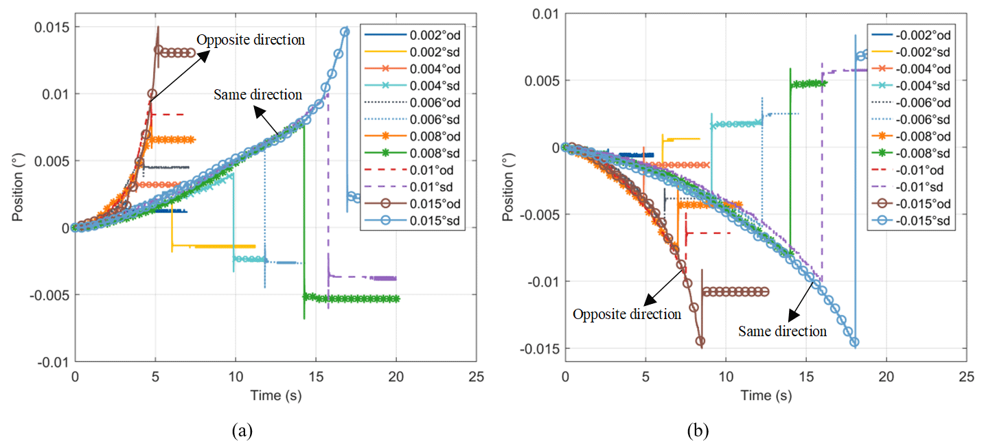
Figure 1Angular position response of DDS under slope command in the forward direction (a) and the reverse direction (b).
The above experimental phenomenon is similar to the prestiction friction phenomenon described by Bazaei and Moallem (2009), but the difference is that this paper obtains a particular prestiction friction phenomenon which is closely related to the state of the system before the motion through the clever design of the experiment. By observing the experimental phenomenon, it is recognized that the system is not in a stationary state after a sudden emergency stop. Instead, it continues to move slowly towards the equilibrium position. This movement is so minuscule that it cannot be detected by current sensors and is therefore considered to be in a stationary state. The slow-moving DDS can be considered a stiffness-damping system with a certain preload. In this system, the energy gradually dissipates over time, and it may take several days for the final dissipation to occur.
Similar to the friction behavior described by the deformation of the bristles between two contact surfaces in the LuGre model, the above phenomenon can also be explained by this theory. The expression for the LuGre model is
where z represents the average deformation of the bristles, TC is the Coulomb friction, TS is the static friction, Ω is the Stribeck velocity, σ0 is the stiffness coefficient, σ1 is the damping coefficient, and σ2 is the viscous coefficient.
After the system is suddenly stopped or the maximum velocity ωmax of the system is reduced to zero within a short time, the average bristle deformation z remains between zero and the maximum value zmax, which is denoted as zstop. Under the weak restoring force of the bristles, the system slowly moves to the equilibrium position, where the average bristle deformation z is zero, and the relationship between angular velocity and bristle deformation is shown in Fig. 2.
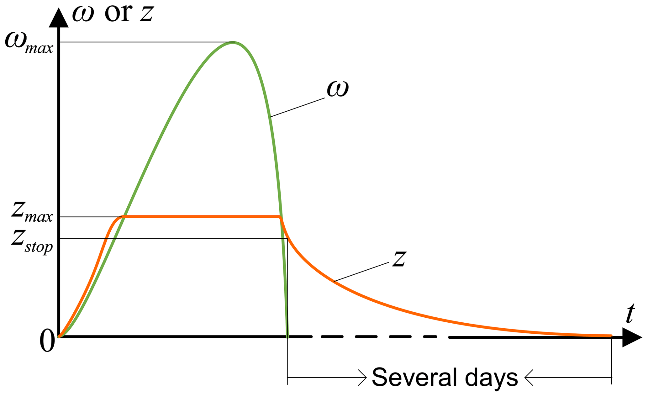
Due to the energy dissipation property of the LuGre model (Canudas-de-Wit and Kelly, 2007), the average deformation of the bristles z and the rate of change are used to describe the variation of friction during the prestiction phase, but after the system stops, the average deformation of the bristles z and the rate of change are forced to zero and cannot exhibit the particular prestiction friction phenomenon.
3.1 Friction model
To accurately describe the friction behavior of the DDS closely related to the state before system operation, this article divides the friction model into pre-sliding and gross-sliding regimes. At extremely low velocities, the friction is in the pre-sliding regime, characterized by the angular velocity and position prior to system halt. Once the system velocity surpasses a predefined threshold, the friction is in the gross-sliding regime, where the friction behavior is governed by the Stribeck model. The established dynamic continuous friction model is shown in Fig. 3, and its key difference from existing friction models lies in the pre-sliding regime. Specifically, it describes the transition process between forward and reverse static friction using a dynamically varying concave function, captures the friction hysteresis phenomenon at zero velocity, and limits the output of the model to static friction using a saturation function.
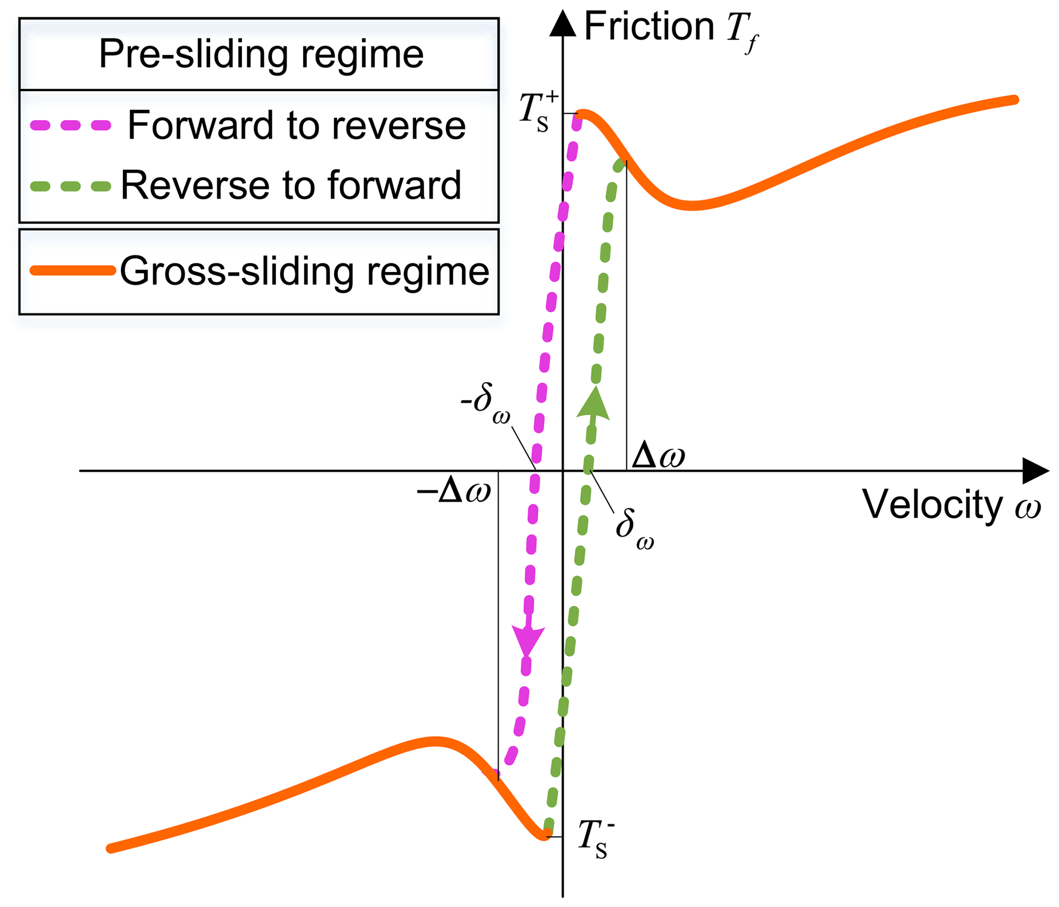
The orange solid line in the figure represents the gross-sliding regime of friction described by the Stribeck model. The pink dashed line and green dashed line represent the pre-sliding regime of friction, where the pink dashed line represents the transition process from forward static friction to reverse static friction, and the green dashed line represents the transition process from reverse static friction to forward static friction. The friction model expression is
where ω represents the angular velocity of the system. and are the static friction, and are the Coulomb friction, B+ and B− are the viscous friction coefficients, and Ω+ and Ω− are the Stribeck velocity parameters. is the velocity variable in the Stribeck model, where . The symbols “+” and “−” represent the forward and reverse directions, respectively. δ is the empirical constant, which is empirically taken as δ=2. The saturation function sat(•) limits its input to the set value. Δω is the angular velocity of the system when the friction regime is switched.
When the system velocity is less than Δω, the system is in the pre-sliding regime, and the friction force is related to a variety of factors. When the system velocity direction changes from reverse to forward, the friction changes gradually from the reverse static friction to the forward static friction , the same when the system velocity direction changes from forward to reverse. In the pre-sliding regime, the trend of the friction is determined by the dynamically varying concave function fc(ω). This concave function satisfies the following equation for any .
In this article, the concave functions fc1(ω) and fc2(ω) are represented by the inverse tangent, expressed as
where k1 and k3 are length coefficients and k2 and k4 are width coefficients that are used to adjust the shape of the concave function. These four parameters are dynamically adjusted according to the system state.
According to the particular prestiction friction phenomenon described in Sect. 2, it is observed that when the velocity of a DDS momentarily reaches zero during its motion, the friction does not become zero. Instead, it becomes zero at a minimal velocity after the direction of motion changes. This minimal velocity is denoted as δω, and it is influenced by the motion state of the system prior to the momentary zero velocity. When the system experiences a sudden emergency stop at high velocity, the value of δω is larger, and when the system comes to a gradual halt at low velocity, the value of δω is smaller or even zero. Therefore, this article describes δω using the following formula:
where ωm is the maximum velocity in the most recent motion, θm is the angle at which the system rotates when it decreases from this maximum velocity to zero, δω has a maximum value denoted as δm (which is a small constant), and δm<Δω.
From the above description, we can obtain
When the system velocity is greater than Δω, the friction is considered the gross-sliding regime, and friction is described by the Stribeck model. To ensure the smoothness of the friction model when switching occurs, is used as the velocity variable in the Stribeck model.
3.2 Friction identification method
The frictional behavior of the system in the gross-sliding regime is described by the Stribeck model, which is characterized by simple and easily identifiable parameters. The DDS is operated in the velocity closed-loop mode, the average velocity and average torque of the motor at a certain velocity command are collected to obtain the friction torque–velocity curve relationship, and the parameters of the Stribeck model are obtained through the least-squares fitting algorithm. In the friction torque–velocity curve relationship, the motor velocity corresponding to the static friction torque is used as the regime-switching velocity from the pre-sliding regime to the gross-sliding regime.
When the system is in the pre-sliding regime, a set of dynamically varying concave functions is used to describe the process of static friction torque between forward and reverse, and the shape of the concave functions is regulated by the length coefficients k1 and k3 and the width coefficients k2 and k4. In the pre-sliding regime, the dynamic variation of the friction torque is determined by two important coordinates, which are (−Δω, and (Δω, , and the length and width coefficients can be determined by combining Eq. (6) with two sets of binary linear equations.
In Eq. (6), the minimal velocity δω is determined by Eq. (5), where θm and ωm are changed in real time according to the system state, and their values are determined based on the angular position, angular velocity, and time of the system. The maximum value δm of the minimal velocity δω can be calculated by referencing the reverse maximum overshoot value at the angular position shown in Fig. 1, which is approximately 0.006°. Consequently, when the system reverses its direction of motion and rotates to achieve this specified angular value, its velocity value is δm.
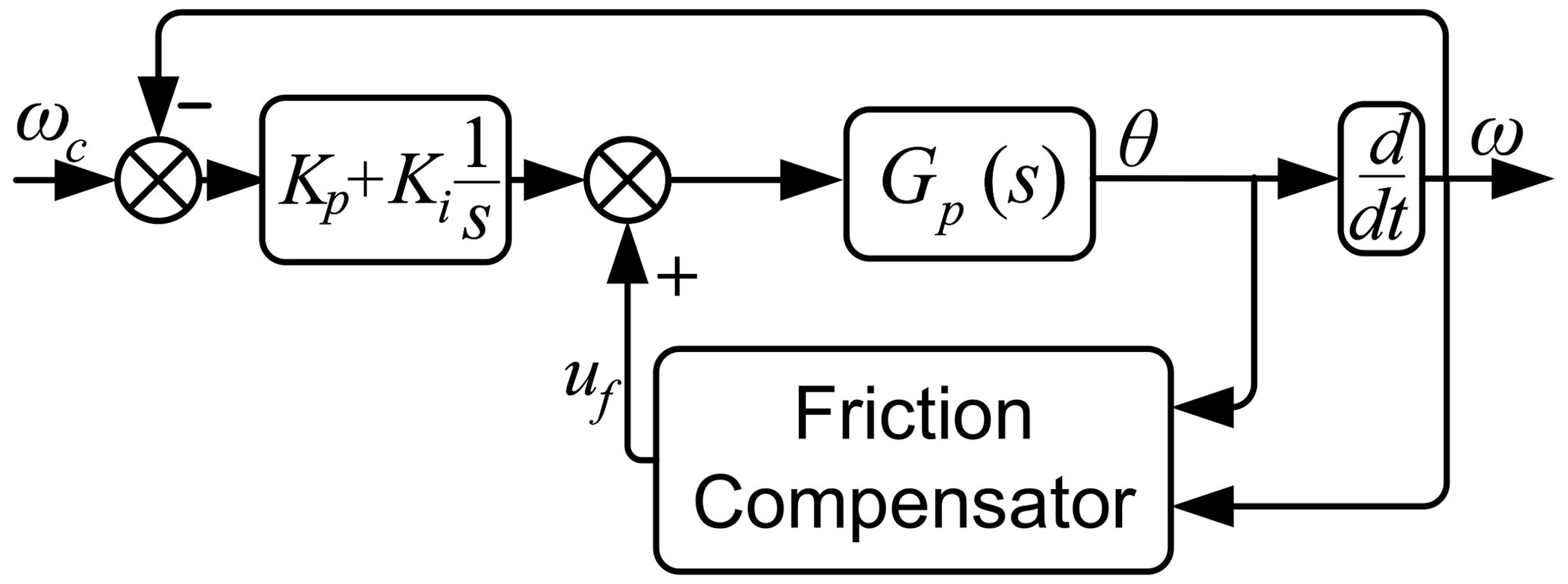
Through experimental tests and simulations, it is found that friction is a key factor that restricts the performance improvement of the DDS. In order to improve the velocity closed-loop control performance of the DDS, the established friction model and the system state information are used to predict the magnitude and direction of the friction torque during the system motion, and the friction model-based compensation method is used to suppress the influence of friction on the system velocity closed-loop performance. The block diagram of the DDS control system with the friction compensation is shown in Fig. 4, which mainly consists of a PI controller and a friction compensator, where Kp and Ki are the proportional parameter and integral parameter, respectively. Gp(s) is the transfer function of the DDS, the inputs of the friction compensator are the output angle θ and angular velocity ω, and the output is the voltage compensation signal uf. In this block diagram, the PI controller, being the simplest and most widely utilized, is employed to eliminate velocity errors, and this controller adjusts the system output by considering both instantaneous velocity errors and accumulated errors over time, effectively reducing steady-state errors and optimizing overall system performance (Wu et al., 2018; Zhang et al., 2014; Wu et al., 2021, 2022). Additionally, a friction compensator is designed based on the established dynamic continuous friction model. This compensator is positioned within the inner loop of the PI controller, allowing it to initially mitigate friction within the DDS.
4.1 PI controller design
The blind adjustment of PI controller parameters often poses challenges in achieving optimal results, as alterations in these parameters influence the servo performance of the system. To address this, the article proposes a method for designing PI controller parameters based on the mechanical parameters, electrical parameters, and servo indicators of the system. This approach aims to standardize the PI controller design, ensuring more consistent and reliable performance. In order to obtain a reasonable value interval for the PI controller parameters to make the system stable, the DDS is simplified to a first-order inertial system, and the system dynamics equations are derived and solved. According to the torque balance equation of the DDS, the following set of differential equations is obtained:
where UC is the input voltage command, ka is the voltage conversion factor of the driver, km is the motor torque coefficient, and Kt=ka km is the total amplification factor. Tm is the driving torque. ω and are the angular velocity and angular acceleration, respectively, of the system. J and B are the total rotational inertia and velocity damping coefficient, respectively, and Tf is the friction torque.
The input velocity command is ωc, and the velocity error e and the integration e0 of the velocity error over time are defined as
Assuming that the proportional parameter of the PI controller is Kp and the integral parameter is Ki, the output signal of the velocity error through the PI controller is
Combining Eqs. (7), (8), (9), and (10), the differential equation for the velocity closed-loop system is obtained as
The state space equation is obtained as
Then the state matrix A is
The characteristic polynomial of the system is
To ensure a good dynamic response performance, it is assumed that the velocity closed-loop system of the DDS is a second-order underdamped system. In this case, the characteristic roots of the characteristic polynomial are a pair of conjugate complex numbers, and their expression is
where ζ is the damping ratio and ωn is the undamped natural frequency.
The dynamic performance index of the second-order underdamped system, evaluated in terms of peak time tp and system damping ζ, has the following relationship:
Combining Eqs. (14), (15), and (16), the expressions of Kp and Ki can be obtained:
According to the standardized design process of the PI controller mentioned above, only some known parameters of the system are needed to easily determine the parameters of the PI controller.
4.2 Friction compensator design
The established dynamic continuous friction model determines the friction torque of the system based on its current and previous states and can describe the friction behavior of the system at zero velocity. Based on this feature, designing the friction compensator based on the established friction model will greatly eliminate system friction and achieve higher velocity control accuracy.
In the pre-sliding regime, the angular position information can be used to determine the friction regime instead of the velocity because of the low accuracy of the system velocity measurement. The angle measured by the encoder is θ(k), the sampling time is T, and k is the kth sampling period of the system. Then the angle difference in a fixed time t0 is
The expression for the friction compensation torque in the pre-sliding regime is
where and the length coefficients and and the width coefficients and can be obtained by the identification method in Sect. 3.2.
In the gross-sliding regime, the encoder differential velocity ω(k) can be used directly, and the friction compensation torque is expressed as
By using the angular position and angular velocity information of the DDS, it is possible to mitigate the impact of system measurement noise to a significant degree. This reduction in noise enables a more accurate calculation of friction compensation torque, thereby facilitating precise friction compensation for the DDS. After obtaining the friction compensation torque, it needs to be converted into the compensation voltage uf, and the relationship between the two is
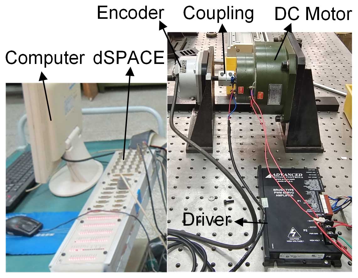
To verify the correctness of the established friction model and the accuracy of the friction compensation-based velocity control, the DDS experimental platform is built as shown in Fig. 5. The DC motor model is 130LCX-2, the peak torque is 8.25 N m, and the motor torque coefficient km is 0.73 N m A−1. The output shaft of the motor is fixedly connected to the input shaft of the encoder through a coupling, and the total rotational inertia J is 0.009 kg m2. The driver model is AMC30A8, and the cutoff frequency of the current closed loop is much larger than the system response frequency, so the current loop part of the driver can be equated to the proportional coefficient, and the voltage conversion factor ka is 0.447 A V−1. The encoder model RON285-18000-0103 provides an angular position output with more than 22-bit resolution through 256 × subdivision. The test system is run on the dSPACE1103 real-time simulation platform with a sampling time setting of 1 ms. The previous debugging experience shows that the peak time tp=0.1 s and the damping ratio ζ=0.707 can meet the dynamic performance of the system. According to Eq. (17), the proportional parameter Kp=1.72 and the integral parameter Ki=54.43 can be calculated.
5.1 Friction parameter identification
To obtain the static friction torque TS and regime-switching velocity Δω, the motor is operated in the current closed-loop state and the control command is a small slope signal, and then the angular position and velocity signals of the encoder are collected. The relationship between the angular position and angular velocity of the system output is shown in Fig. 6. From the figure, when the output angle of the system is greater than 0.048°, the output velocity is 0.39° s−1 (5 times the velocity resolution), which obviously shows the trend of accelerated motion and at this time the friction regime through the transition from the pre-sliding regime to the gross-sliding regime. Therefore, the angular velocity corresponding to this point is set as the regime-switching velocity Δω, and the corresponding friction torque is the static friction torque TS. Due to the extremely low output velocity of the system, the driving torque of the motor can be equivalent to the friction torque of the system.
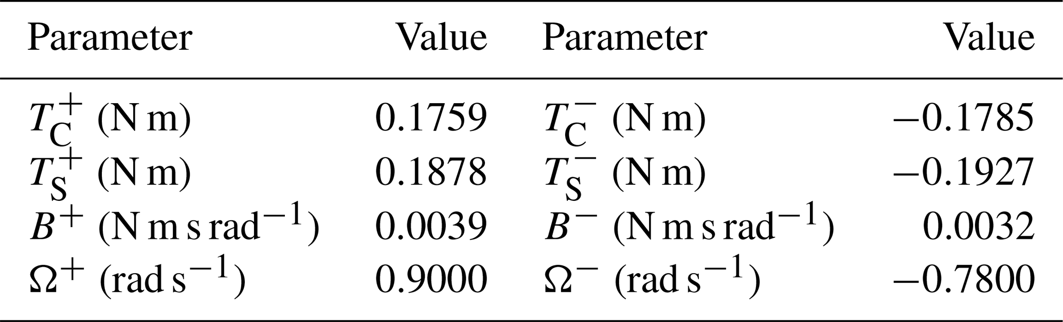
When the friction of the system is in the gross-sliding regime, there is a Stribeck curve relationship between the friction torque and velocity, allowing the system to operate in a velocity closed-loop mode and achieve uniform operation at different velocities. The motor current signal is used as a reference value for the friction torque at the current velocity, and the Stribeck model parameters are identified through curve fitting as shown in Table 1, which can be used for subsequent velocity control based on friction compensation.
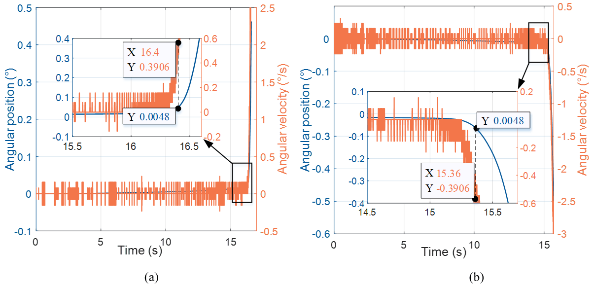
Figure 6Output response of the DDS under slope command in (a) the forward direction and (b) the reverse direction.
5.2 Sine-tracking experiment
The proposed dynamic continuous friction model focuses on describing the friction behavior at low velocity and velocity past zero. To test the effectiveness of the established friction model and the compensation method, the output velocity of the DDS is made to track a sine signal, and the PI controller, the Stribeck friction compensation method (PI + Stribeck), and the proposed friction compensation method are compared at different amplitudes and different frequencies of the sinusoidal signal, respectively. The amplitude and frequency of the sinusoidal signals are 6.28° s−1 1 Hz, 6.28° s−1 0.5 Hz, 10° s−1 1 Hz, and 20° s−1 0.5 Hz, respectively. The experimental results of the DDS are shown in Fig. 7.
From the figure, when using the PI controller and the Stribeck friction compensation method, the output velocity of the DDS shows a significant tracking error in the low-velocity region after the velocity passes zero, manifested as the error peak phenomenon in the velocity error graph and indicating the existence of overcompensation. The proposed friction compensation method significantly reduces the velocity-tracking error in the low-velocity region after the velocity passes zero, indicating the effectiveness of the proposed friction compensation method and the accuracy of the established friction model in describing low-velocity friction behavior.
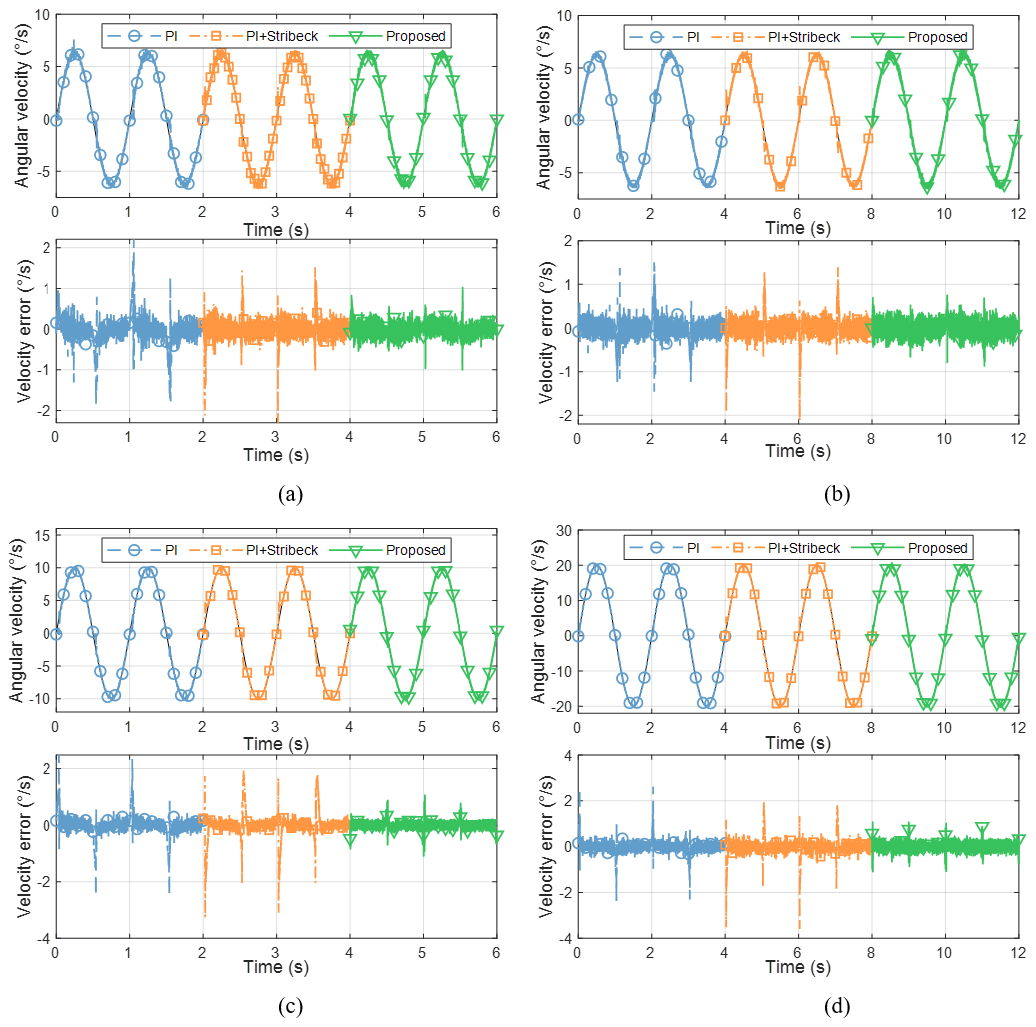
Figure 7Performance comparison of three control methods with different input signals: (a) 6.28° s−1 1 Hz, (b) 6.28° s−1 0.5 Hz, (c) 10° s−1 1 Hz, and (d) 20° s−1 0.5 Hz.
With the increasing amplitude of the sine signal, the magnitude of the velocity error using the Stribeck friction compensation method is also increasing. Different from the proposed dynamic continuous friction model, the Stribeck model is a static model, and the discontinuity of the Stribeck model at zero velocity and the characteristic of not recording the operating state of the system lead to a more serious velocity error peak phenomenon (Fu et al., 2017; Tjahjowidodo et al., 2007).
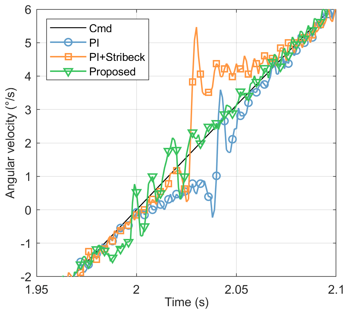
In order to visually analyze the control effect of the proposed friction model and compensation method, the details of the sine tracking of the DDS at velocity past zero are enlarged, as shown in Fig. 8. The proposed friction compensation method has some velocity fluctuation when the system velocity passes zero, and the velocity-tracking effect is obviously better. Thanks to the fact that the proposed dynamic continuous friction model has the characteristic of recording the system operation state all the time, the friction in the system is calculated and compensated for when the velocity is briefly reduced to zero, which realizes the “prior compensation” before the system velocity passes zero, and the overcompensation is suppressed to the maximum extent.
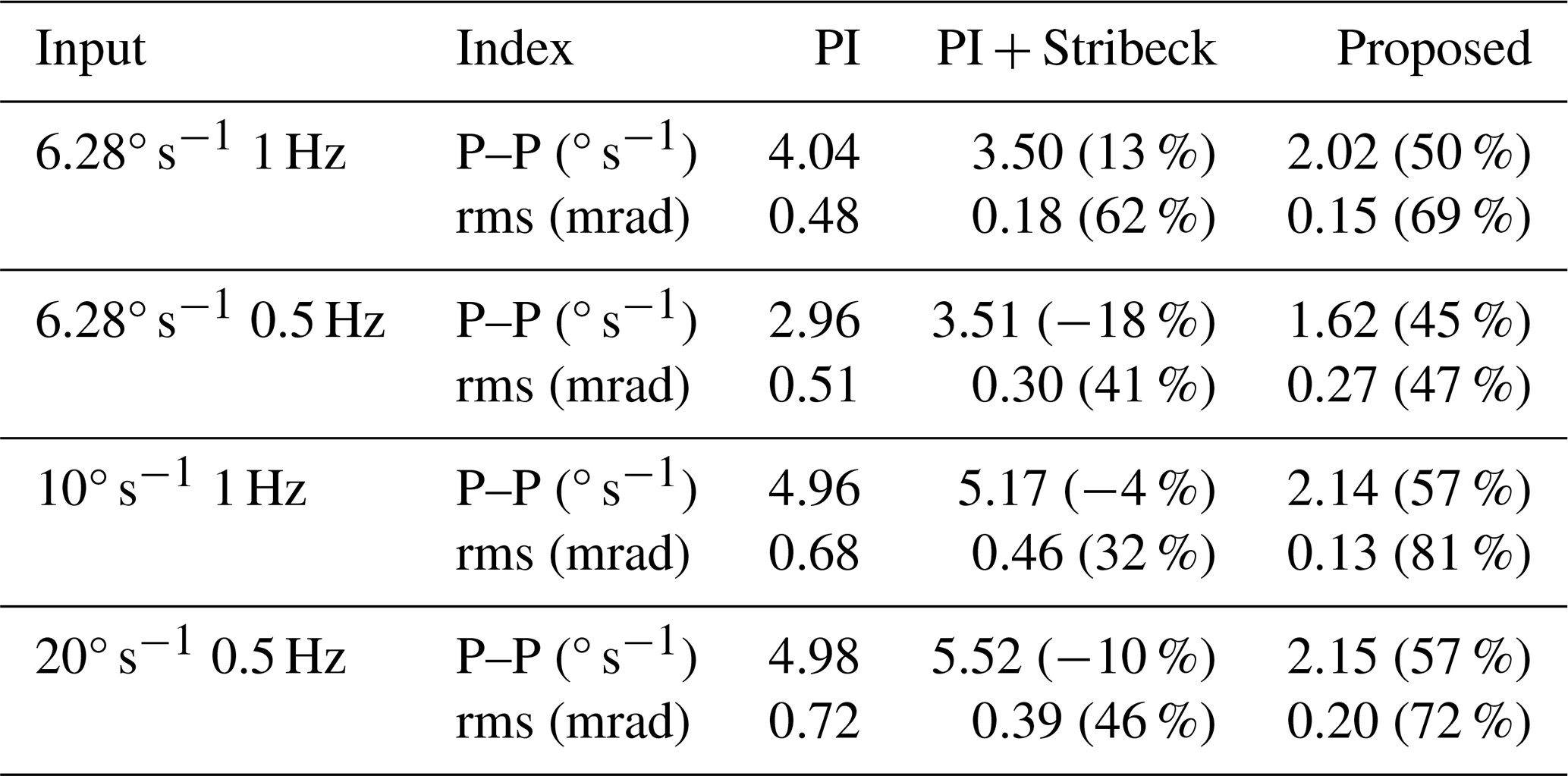
The peak-to-peak (P–P) value of the velocity error and the root-mean-square (rms) value of the velocity error integral are used as evaluation indexes to quantitatively determine the tracking effect of the proposed friction compensation method under different sine signals. The calculated results of the evaluation indexes for the DDS under the three control methods are calculated separately, as shown in Table 2.
The evaluation indexes of the sine tracking of the DDS under the three control methods are listed in Table 2, and the percentages in parentheses indicate the degree of improvement compared with the PI controller. Compared with the PI controller, the P–P value of the velocity error is not reduced with the Stribeck friction compensation method, but the rms value is improved significantly, while the application of the proposed friction compensation method results in a significant improvement in both indexes, with a 57 % reduction in the P–P value and an 81 % reduction in the rms value in the optimal tracking. Compared with the Stribeck friction compensation method, the P–P value of the proposed friction compensation method is significantly reduced by a maximum of 61.1 %, and the rms value is reduced by 71.7 %. The minimum P–P value of the proposed friction compensation method is 1.62° s−1, and the minimum rms value reaches 0.13 mrad, achieving a high level of control accuracy for the DDS.
According to the different angular position responses of the DDS to the same input signal after a sudden emergency stop, the system exhibits a particular prestiction friction phenomenon, which leads to the conclusion that the friction is not zero at the zero velocity of the system. Based on this, this paper proposes a dynamic continuous friction model consisting of a pre-sliding regime and a gross-sliding regime, which differs from the existing friction model in that it utilizes the angular velocity and angular position information of the system before the velocity briefly reaches zero, and it describes the transition process between forward and reverse static friction with a dynamically changing concave function, thus describing the friction hysteresis phenomenon at zero velocity.
Based on the established dynamic and continuous friction model, a friction compensation method for the DDS is developed in velocity control mode. The superior performance of this proposed friction compensation method is demonstrated through sine-tracking experiments. When compared to the PI controller, the proposed method achieves a reduction in the P–P value by 57 %, and the rms value is reduced by 81 %. Compared with the Stribeck friction compensation method, the proposed method further reduces the maximum P–P value by 61.1 % and the rms value by 71.7 %, with the minimum rms value reaching an impressive 0.13 mrad, thereby enabling high-precision velocity control of the DDS.
The data are available upon request from the corresponding author.
DF and XX proposed the ideas and specific research content of the paper. BL, BY, and YL conducted the controller design and experiments. BL analyzed the experimental data and wrote the manuscript. DF and XX reviewed and revised the manuscript.
The contact author has declared that none of the authors has any competing interests.
Publisher’s note: Copernicus Publications remains neutral with regard to jurisdictional claims made in the text, published maps, institutional affiliations, or any other geographical representation in this paper. While Copernicus Publications makes every effort to include appropriate place names, the final responsibility lies with the authors.
The authors would like to thank the support from the key laboratory of science and technology, National University of Defense Technology (NUDT).
This research has been supported by the National Natural Science Foundation of China (grant nos. 5230507 and U19A2072).
This paper was edited by Jinguo Liu and reviewed by Saygin Ahmed, Jichun Wu, and four anonymous referees.
Bazaei, A. and Moallem, M.: Prestiction Friction Modeling and Position Control in an Actuated Rotary Arm, IEEE T. Instrum. Meas., 59, 131–139, https://doi.org/10.1109/TIM.2009.2022109, 2009.
Canudas-de-Wit, C. and Kelly, R.: Passivity Analysis of a Motion Control for Robot Manipulators with Dynamic Friction, Asian J. Control, 9, 30–36, https://doi.org/10.1111/j.1934-6093.2007.tb00301.x, 2007.
Feng, H., Qiao, W., Yin, C., Yu, H., and Cao, D.: Identification and compensation of non-linear friction for a electro-hydraulic system, Mech. Mach. Theory, 141, 1–13, https://doi.org/10.1016/j.mechmachtheory.2019.07.004, 2019.
Feng, H., Yin, C., and Cao, D.: Trajectory Tracking of an Electro-Hydraulic Servo System With an New Friction Model-Based Compensation, IEEE/ASME Trans. Mechatron., 28, 1–10, https://doi.org/10.1109/TMECH.2022.3201283, 2022.
Fu, J., Maré, J.-C., and Fu, Y.: Modelling and simulation of flight control electromechanical actuators with special focus on model architecting, multidisciplinary effects and power flows, Chinese J. Aeronaut., 30, 47–65, https://doi.org/10.1016/j.cja.2016.07.006, 2017.
Hu, X., Han, S., Liu, Y., and Wang, H.: Two-Axis Optoelectronic Stabilized Platform Based on Active Disturbance Rejection Controller with LuGre Friction Model, Electronics, 12, 1261, https://doi.org/10.3390/electronics12051261, 2023.
Huang, S., Liang, W., and Tan, K. K.: Intelligent Friction Compensation: A Review, IEEE/ASME Trans. Mechatron., 24, 1763–1774, https://doi.org/10.1109/TMECH.2019.2916665, 2019.
Li, X., Yao, J., and Zhou, C.: Output feedback adaptive robust control of hydraulic actuator with friction and model uncertainty compensation, J. Frankl. Inst., 354, 5328–5349, https://doi.org/10.1016/j.jfranklin.2017.06.020, 2017.
Liu, X., Li, Y., Cheng, Y., and Cai, Y.: Sparse identification for ball-screw drives considering position-dependent dynamics and nonlinear friction, Robot. Cim.-Int. Manuf., 81, 102486, https://doi.org/10.1016/j.rcim.2022.102486, 2023.
Liu, Y., Feng, X., Li, P., Li, Y., Su, Z., Liu, H., Lu, Z., and Yao, M.: Modeling, Identification, and Compensation Control of Friction for a Novel Dual-Drive Hydrostatic Lead Screw Micro-Feed System, Machines, 10, 914, https://doi.org/10.3390/machines10100914, 2022.
Makkar, C., Dixon, W. E., Sawyer, W. G., and Hu, G.: A new continuously differentiable friction model for control systems design, Proceedings, 2005 IEEE/ASME International Conference on Advanced Intelligent Mechatronics., 600–605, https://doi.org/10.1109/AIM.2005.1511048, 2005.
Marques, F., Flores, P., Pimenta Claro, J. C., and Lankarani, H. M.: A survey and comparison of several friction force models for dynamic analysis of multibody mechanical systems, Nonlinear Dyn., 86, 1407–1443, https://doi.org/10.1007/s11071-016-2999-3, 2016.
Marques, F., Woliński, Ł., Wojtyra, M., Flores, P., and Lankarani, H. M.: An investigation of a novel LuGre-based friction force model, Mech. Mach. Theory, 166, 104493, https://doi.org/10.1016/j.mechmachtheory.2021.104493, 2021.
Marton, L. and Lantos, B.: Modeling, Identification, and Compensation of Stick-Slip Friction, IEEE Trans. Ind. Electron., 54, 511–521, https://doi.org/10.1109/TIE.2006.888804, 2007.
Márton, L. and Lantos, B.: Control of mechanical systems with Stribeck friction and backlash, Syst. Control Lett., 58, 141–147, https://doi.org/10.1016/j.sysconle.2008.10.001, 2009.
Pennestrì, E., Rossi, V., Salvini, P., and Valentini, P. P.: Review and comparison of dry friction force models, Nonlinear Dyn., 83, 1785–1801, https://doi.org/10.1007/s11071-015-2485-3, 2016.
Ruderman, M.: Tracking Control of Motor Drives Using Feedforward Friction Observer, IEEE Trans. Ind. Electron., 61, 3727–3735, https://doi.org/10.1109/TIE.2013.2264786, 2014.
Ruderman, M. and Bertram, T.: Two-state dynamic friction model with elasto-plasticity, Mech. Syst. Signal Proces., 39, 316–332, https://doi.org/10.1016/j.ymssp.2013.03.010, 2013.
Thenozhi, S., Sánchez, A. C., and Rodríguez-Reséndiz, J.: A Contraction Theory-Based Tracking Control Design With Friction Identification and Compensation, IEEE T. Ind. Electron., 69, 6111–6120, https://doi.org/10.1109/TIE.2021.3094456, 2022.
Tjahjowidodo, T., Al-Bender, F., Van Brussel, H., and Symens, W.: Friction characterization and compensation in electro-mechanical systems, J. Sound Vib., 308, 632–646, https://doi.org/10.1016/j.jsv.2007.03.075, 2007.
Wan, M., Dai, J., Zhang, W.-H., Xiao, Q.-B., and Qin, X.-B.: Adaptive feed-forward friction compensation through developing an asymmetrical dynamic friction model, Mech. Mach. Theory, 170, 104691, https://doi.org/10.1016/j.mechmachtheory.2021.104691, 2022.
Wang, C., Peng, J., and Pan, J.: A Novel Friction Compensation Method based on Stribeck Model with Fuzzy Filter for PMSM Servo Systems, IEEE T. Ind. Electron., 70, 12124–12133, https://doi.org/10.1109/TIE.2022.3232667, 2023.
Wu, J., Yu, G., Gao, Y., and Wang, L.: Mechatronics modeling and vibration analysis of a 2-DOF parallel manipulator in a 5-DOF hybrid machine tool, Mech. Mach. Theory, 121, 430–445, https://doi.org/10.1016/j.mechmachtheory.2017.10.023, 2018.
Wu, J., Zhang, B., Wang, L., and Yu, G.: An iterative learning method for realizing accurate dynamic feedforward control of an industrial hybrid robot, Sci. China Technol. Sci., 64, 1177–1188, https://doi.org/10.1007/s11431-020-1738-5, 2021.
Wu, J., Song, Y., Liu, Z., and Li, G.: A modified similitude analysis method for the electro-mechanical performances of a parallel manipulator to solve the control period mismatch problem, Sci. China Technol. Sci., 65, 541–552, https://doi.org/10.1007/s11431-021-1955-8, 2022.
Wu, Y., Wang, Z., Li, Y., Chen, W., Du, R., and Chen, Q.: Characteristic Modeling and Control of Servo Systems with Backlash and Friction, Mathematical Problems in Engineering, 2014, 1–21, https://doi.org/10.1155/2014/328450, 2014.
Yao, J., Deng, W., and Jiao, Z.: Adaptive Control of Hydraulic Actuators With LuGre Model-Based Friction Compensation, IEEE Trans. Ind. Electron., 62, 6469–6477, https://doi.org/10.1109/TIE.2015.2423660, 2015.
Yin, N., Xing, Z., He, K., and Zhang, Z.: Tribo-informatics approaches in tribology research: A review, Friction, 11, 1–22, https://doi.org/10.1007/s40544-022-0596-7, 2023.
Yu, H., Gao, H., Deng, H., Yuan, S., and Zhang, L.: Synchronization Control With Adaptive Friction Compensation of Treadmill-Based Testing Apparatus for Wheeled Planetary Rover, IEEE T. Ind. Electron., 69, 592–603, https://doi.org/10.1109/TIE.2021.3050366, 2022.
Zhang, W., Li, M., Gao, Y., and Chen, Y. Q.: Periodic adaptive learning control of PMSM servo system with LuGre model-based friction compensation, Mech. Mach. Theory, 167, 104561, https://doi.org/10.1016/j.mechmachtheory.2021.104561, 2022.
Zhang, Z., Li, Z., Zhou, Q., Zhang, L., and Fan, D.: Application in prestiction friction compensation for angular velocity loop of inertially stabilized platforms, Chin. J. Aeronaut., 27, 655–662, https://doi.org/10.1016/j.cja.2014.04.026, 2014.