Multi-robot consensus formation based on virtual spring obstacle avoidance

A systematic improvement of the multi-robot formation control algorithm has been developed to address multi-robot formation instability. First, a static obstacle avoidance model based on spring force mapping is proposed, followed by an analysis of the influence of static and dynamic obstacles on the processing of multi-robot cooperative motion. Second, a leader is introduced to the formation to save computational costs. Third, the Velocity Obstacle (VO) algorithm is improved to resolve robot collisions during the dynamic mobility process caused by the increased number of multi-robot formations. Simultaneously, the dynamic speed limit function based on the position error for formation keeping is established. Finally, simulation experiments are carried out. Results show that when 5-robot and 20-robot formations were compared in the environment without dynamic conflict, the average value of the position error of 20-robot formations only increased by 39.47 %, and the average value of the path length did not differ significantly. In the dynamic conflict environment, the maximum position error of 20-robot formations increases by 73.03 % and the path length average value increases by 7.69 %. Our proposed method can control the motion of multiple robots in both conflict-free and conflict-filled environments, resulting in an effective motion planning scheme.

1 Introduction

A multi-robot system (MRS) is gradually being used in rescue operations such as firefighting, mine clearing, hazardous waste collection, and workshop handling (Li et al., 2020). An MRS demonstrates its benefits, and it establishes new needs for suitable control methods, including more rational task allocation, motion planning, and formation control (Roszkowska, 2018). The goal of MRS operation is to utilize many robots to accomplish more complex jobs and avoid static and dynamic obstacles more efficiently based on shared basis information (Niu et al., 2020). However, as the number of robots increases, the robots begin to interfere with one another. This interference impairs the MRS's ability to improve its operating efficiency (Mao et al., 2018).

Multi-robot formation (MRF) is one of the effective ways of improving the motion efficiency of an MRS (Zhang et al., 2020). MRF maintains geometric relationships between robots based on task needs, which was intensively investigated recently. The motion consistency of multi-robots is the core problem of MRF optimization control. MRF control can be divided into an artificial potential field method, a behavior-based method, a leader–follower method (Dai and Lee, 2012), and graph theory. Song et al. (2014) proposed a collaborative control algorithm based on the artificial potential field method. Three alternative functions were developed to meet a task's various requirements for consistent control and collision avoidance. However, the method of Song is less robust to dynamic changes in the environment. The zero-space behavior control method was proposed by Arrichiello et al. (2010) and has a precise mathematical description to ensure the execution of tasks as a priority. Soleymani and Saghafi (2010) proposed a combined method of double-loop control and Lyapunov systems directed to keep MRF. Conflict resolution and individual cooperation could be realized based on the combined method to solve individual prediction and ease the computational complexity. Ji et al. (2009) studied the connectivity and controllability of graph topology in MRS and gave the necessary and sufficient conditions of system controllability according to the eigenvectors of subgraphs. Li and Spong (2014) proposed a geometric decomposition method for solving the problem of coupling control of speed and position in an MRS. Jafari et al. (2011) discussed the convergence of the multi-leader system and analyzed the controllability conditions of the multi-agent structure using graph theory. Obviously, when the number of robots increases, especially when the robots have the nature of group movement, the motion among robots on the stage will cause dynamic obstacles among robots. Therefore, when the number of robots is further expanded, the above research will become a bottleneck.

At present, the most often used techniques for resolving individual behavior problems in groups are traffic regulation, priority setting, and rate adjustment. Wenmin et al. (2015) proposed an improved priority access control algorithm for emergency vehicles at intersections for vehicle road coordination systems. However, this strategy may result in congestion at crossings. Yang et al. (2017) investigated the possible risk and multi-obstacle problem using the velocity obstacle approach. However, the model assumes a constant speed for an unoccupied aerial vehicle (UAV), and the application scenarios are constrained. Durand and Barnier (2015) first established the speed obstacle approach and then used this information to solve the aircraft conflict detection problem. They developed a technique in conjunction with a self-separation algorithm for implementing the multi-robot system in a flight environment. Allignol et al. (2017) then suggested a technique of analysis based on location and velocity. Goss et al. (2004) concentrated on the issue of track restoration following the aircraft's release and redirected it to its original destination without provoking additional issues. Nevertheless, the methods outlined above approach each robot as an adversary, resulting in a lack of collaboration and conflict resolution between robots. Remarkably, the motion objectives of the robots in the preceding systems are not consistent. As a result, using the aforementioned methodologies to cooperate with and control multiple robots is challenging.

In general, the MRSs investigated previously are comprised of three to five robots in formation. Hence, when the formation contains more robots, interference between robots becomes a significant problem impeding the formation's motion. Additionally, it is not preferable to build a formation for the other robots except the leader, which is a dynamic impediment to one another. For consistent motion, the robots behind the space position can use the path experience of the former robots. Obviously, the motion efficiency of the robots is improved, and the efficiency of the multi-robot motion is improved. The following are the major contributions for the proposed paper. (1) A method combining graph theory with the leader and followers is proposed to solve the problem of multi-robot formation conflict. Each follower shares information with both the leader and the adjacent robots to achieve formation consistency. (2) Unique obstacle avoidance for the distance virtual spring robots is implemented. (3) The dynamic speed limit method is used to prevent the virtual spring force from being too large to cause the robots to deviate from the formation avoidance. (4) The rate adjustment method is used to resolve the conflict between MRF and other robots.

2 Formation model of an improved leader–follower algorithm for dynamic obstacle avoidance

2.1 Multi-robot model

A robot's coordinated control strategy is based on the exchange of local information to maintain the expected formation and speed. Therefore, the real-time state information of the MRS is defined according to information topology theory. Using the basic concept of graph theory, for n robots, set $\mathbf{R}=\left\{{\mathit{r}}_{\mathbf{1}},{\mathit{r}}_{\mathbf{2}},\mathrm{\dots },{\mathit{r}}_{\mathit{i}},\mathrm{\dots },{\mathit{r}}_{\mathit{n}}\right\}$, define $\mathit{\delta }=\left(\mathbf{G},\mathbf{E},\mathbf{O}\right)$ as an n-order weighted digraph, and set nodes $\mathbf{O}=\left\{{\mathit{o}}_{\mathbf{1}},{\mathit{o}}_{\mathbf{2}},\mathrm{\dots },{\mathit{o}}_{\mathit{n}}\right\}$. The set of the directed edge e and the weighted adjacency matrix is $\mathbf{G}=(g_{ij}{)}_{n\times n}$. The directed edge e_ij in the network is represented by an ordered pair of nodes (o_i,o_j). The directed path from node o_i to node o_j in G is an edge sequence (o_i,o_j) in a directed network (Durand and Barnier, 2015).

An adjacency matrix A is introduced to represent the relationship between nodes and edge information connectivity among nodes (i.e., between robots and their adjacent robots). The value of element a_ij in A is provided in Eq. (1):

$$\begin{array}{}\text{(1)}& a_{ij}=\mathrm{1},\left({\mathit{o}}_{\mathit{i}},{\mathit{o}}_{\mathit{j}}\right)\in E\text{or}\mathrm{0}\text{otherwise}.\end{array}$$

$\mathbf{L}=\mathbf{D}-\mathbf{A}$ represents the Laplacian matrix of the topological graph. The number of eigenvalues 0 of the matrix is the number of connected regions of the graph (the amount of information connected among robots and other robots). The A matrix $\mathbf{L}=[l_{ij}{]}_{n\times n}$ is obtained. The definition of L_ij is shown in Eq. (2). The degree matrix D represents each point on the graph (i.e., the number of signals that the robot could send), and D∈R^m is a diagonal matrix. The degree matrix D is obtained by adding the elements of each column of matrix A and placing the sum values of each column element in the corresponding position of the diagonal line of the matrix.

$$\begin{array}{}\text{(2)}& l_{ij}=\sum _{j=\mathrm{1}}{a}_{ij},i=j\text{or}{l}_{ij}=-a_{ij},i\ne j\end{array}$$

For the formation system with n robots, the second-order dynamic model of robot i can be shown in Eq. (3).

$$\begin{array}{}\text{(3)}& \left\{\begin{array}{l}{p}_i(t+\mathrm{1})=p_i\left(t\right)+T{v}_i\left(t\right)\\ v_i(t+\mathrm{1})=v_i\left(t\right)+T{u}_i\left(t\right)\end{array}\right.\end{array}$$

t and t+1 represent the time relationship between the current and the next time, p_i(t) and p_i(t+1) represent the position of robot i in two-dimensional space, v_i(t) and v_i(t+1) represent the two-dimensional velocity vector of robot i, u_i(t) is the input control quantity of robot i, and t is the sampling period.

The expected relative distance error among the followers and the leader is added to the conventional formation consistency control rate to achieve the formation control. The parameters in Eq. (4) have the same meaning as those in Eq. (3). According to Eq. (1), the input control quantity of robot i is obtained as shown in Eq. (4).

$$\begin{array}{}\text{(4)}& \begin{array}{rl}{u}_i\left(t\right)=-\left(L_{ij}\otimes I_n\right)[& \left(p_i\left(t\right)-p_j\left(t\right)\right)-\left(E_i\left(t\right)-E_j\left(t\right)\right)\\ & +\left(v_i\left(t\right)-v_j\left(t\right)\right)]\end{array}\end{array}$$

I_n is the n-dimensional identity matrix and the expected relative spacing error of each robot in the E formation. To make the formation robot i reach the desired position and speed, it follows the leader, as shown in Eq. (5).

$$\begin{array}{}\text{(5)}& \left\{\begin{array}{l}{lim}_{t\to \mathrm{\infty }}∥p_i\left(t\right)-p_l\left(t\right)∥=D_E\\ \underset{t\to \mathrm{\infty }}{lim}∥v_i\left(t\right)-v_l\left(t\right)∥=\mathrm{0}\end{array}\right.\end{array}$$

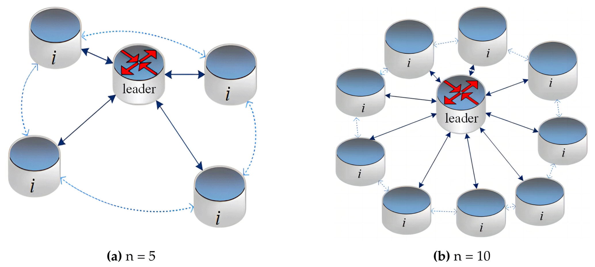
p_l(t) and v_l(t) represent the leader's position and speed at time t, respectively. Figure 1 shows a low computational complexity topology, (a) taking 5 robots and (b) taking 10 robots in the system as examples. The leader is marked as a leader, and the follower robot is marked with i. In a limited number of multi-robot systems, this structure could provide stable formation at the same speed. The followers could obtain the speed and position information of a leader and realize the information exchange among adjacent followers, laying the groundwork for data interchange and computation necessary to resolve the conflict.

Figure 1 Topology of communication between robots.

The velocity of the formation leader (t+1) is determined by the distance d_{l_obj}(t) (obj in the target position) and angle from the aiming position at time t. The speed is proportional to the distance; i.e., the greater the distance, the greater the speed. According to the angle θ, the velocity components on the x and y axes are obtained as shown in Eq. (6), where α is a coefficient robot acceleration, electric quantity, and follower resultant force.

$$\begin{array}{}\text{(6)}& \left\{\begin{array}{l}{v}_l^y(t+\mathrm{1})=\mathit{\alpha }\times d_{l\mathit{\_}\mathrm{obj}}\left(t\right)\times \sin \mathit{\theta }\\ v_l^x(t+\mathrm{1})=\mathit{\alpha }\times d_{l\mathit{\_}\mathrm{obj}}\left(t\right)\times \cos \mathit{\theta }\end{array}\right.\end{array}$$

In practice, the robot is located at the farthest distance of the target at the beginning of the task. Then, the initial speed of the leader is $v_l\left(\mathrm{0}\right)=v_{max}$, and v_max is the maximum speed of the robot.

2.2 Static obstacle avoidance model based on spring force

The spring force model is improved in this article based on the formation. The speed limit enhances formation retention, obstacle avoidance precision, and movement speed even further.

(1) The virtual spring force model

For the fixed obstacle, the distance between the robots and the obstacle is expressed as a spring force, which is proportional to the distance between the robots and the obstacle. Based on the x and y axes, the relationship between spring force f^x(t)f^y(t) and the position distance of the robot and obstacle is shown in Eq. (7).

$$\begin{array}{}\text{(7)}& \left\{\begin{array}{l}\begin{array}{rl}{f}^x\left(t\right)& ={\displaystyle \frac{\mathrm{1}}{{\left(d_{l\mathit{\_}\mathrm{obs}}\left(t\right)\right)}^{\mathrm{3}}}}\times \left(p_i^x\left(t\right)-p_{\mathrm{obs}}^x\left(t\right)\right)\\ & +\sum _{i=\mathrm{1}}^n{\displaystyle \frac{\mathrm{1}}{{\left(d_{ij}\left(t\right)\right)}^{\mathrm{3}}}}\times \left(p_i^x\left(t\right)-p_j^x\left(t\right)\right)& i\ne j\end{array}\\ \begin{array}{rl}{f}^y\left(t\right)& ={\displaystyle \frac{\mathrm{1}}{{\left(d_{l\mathit{\_}\mathrm{obs}}\left(t\right)\right)}^{\mathrm{3}}}}\times \left(p_i^y\left(t\right)-p_{\mathrm{obs}}^y\left(t\right)\right)\\ & +\sum _{i=\mathrm{1}}^n{\displaystyle \frac{\mathrm{1}}{{\left(d_{ij}\left(t\right)\right)}^{\mathrm{3}}}}\times \left(p_i^y\left(t\right)-p_j^y\left(t\right)\right)& i\ne j\end{array}\end{array}\right.\end{array}$$

d_{l_obs}(t) is the distance between the leader and obstacle at time t (obs represents the position of the target obstacle), d_ij(t) is the distance between the robots at time t, and the power value of (d_{l_obs}(t))³ and (d_ij(t))³ represents the elastic coefficient. The experimental results show that the third power is the best. x and y represent the components of the values on the x and y axes, respectively.

(2) Leader obstacle avoidance

During the formation obstacle avoidance process, the leader selects the obstacle avoidance path first (Han et al., 2019). The obstacle avoidance speed is related to the virtual force and initial velocity of the spring. The velocities $v_{l\mathit{\_}\mathrm{a}}^x$ and $v_{l\mathit{\_}\mathrm{a}}^y$ in the x and y directions are shown in Eq. (8).

$$\begin{array}{}\text{(8)}& \left\{\begin{array}{l}{v}_{l\mathit{\_}\mathrm{a}}^x(t+\mathrm{1})=v_l^x\left(t\right)+f^x\\ v_{l\mathit{\_}\mathrm{a}}^y(t+\mathrm{1})=v_l^y\left(t\right)+f^y\end{array}\right.\end{array}$$

(3) Follower obstacle avoidance

The followers follow the leader to the desired point during the formation movement. In our method, the formation shape is not a straight line. Because followers cannot safely avoid barriers when following the leader directly, they must avoid them while following the leader. When followers avoid impediments, the virtual spring force generated by the obstacle and the speed of followers is affected by the leader's speed since the followers need to consider the consensus with the leader. The motion speed of the robot in the x and y directions is as follows.

$$\begin{array}{}\text{(9)}& \left\{\begin{array}{l}{v}_{f_{i\mathit{\_}\mathrm{a}}}^x(t+\mathrm{1})=v_{l\mathit{\_}\mathrm{a}}^x(t+\mathrm{1})+v_{f_i}^x(t+\mathrm{1})+f^x\\ v_{f_{i\mathit{\_}\mathrm{a}}}^y(t+\mathrm{1})=v_{l\mathit{\_}\mathrm{a}}^y(t+\mathrm{1})+v_{f_i}^y(t+\mathrm{1})+f^y\end{array}\right.\end{array}$$

In Eq. (9), $v_{f_{i\mathit{\_}\mathrm{a}}}^x$ and $v_{f_{i\mathit{\_}\mathrm{a}}}^y$ are the obstacle avoidance speed of the follower in the x and y directions, respectively.

(4) Formation consistency

To maintain consistency in the formation movement, the speed of followers should be adjusted in relation to the position difference between the ideal and the actual. The true value is determined by the follower and the leader. By lowering the perceived value of errors, followers can become more consistent with the leader. The model is shown in Eqs. (10) and (11).

$$\begin{array}{}\text{(10)}& \left\{\begin{array}{c}{v}_{f_i}^x(t+\mathrm{1})=\mathit{\beta }\times E_s\left(t\right)\times \cos \mathit{\varphi }\\ v_{f_i}^y(t+\mathrm{1})=\mathit{\beta }\times E_s\left(t\right)\times \sin \mathit{\varphi }\end{array}\right.\end{array}$$

$$\begin{array}{}\text{(11)}& E_s\left(t\right)=\sqrt{{\left(\sum _{i=\mathrm{1}}^n{u}_x\left(t\right)\right)}^{\mathrm{2}}+{\left(\sum _{i=\mathrm{1}}^n{u}_y\left(t\right)\right)}^{\mathrm{2}}}\end{array}$$

$v_{f_i}^x$ and $v_{f_i}^y$ are the velocities of the follower i in the x and y directions, in agreement with the leader. E_s are the position errors among the leader and the followers. ϕ is the angle between robot position i and the x axis, and β is the adjustment coefficient of consistent motion.

(5) The dynamic speed-limiting function

Higher speed and acceleration make robot deviation formation easy and recovery difficult. However, limited speed or acceleration reduces their flexibility. Solving the problem, a dynamic speed restriction is indicated in Eqs. (12) and (13).

$$\begin{array}{}\text{(12)}& \mathrm{\Delta }{v}_i(t+\mathrm{1})=\mathit{\epsilon }\cdot v_{max},\mathit{\epsilon }={\displaystyle \frac{E_i\left(t\right)-E_i(t-\mathrm{1})}{E_i\left(t\right)}}\end{array}$$

$$\begin{array}{}\text{(13)}& v_i(t+\mathrm{1})=\min \left[v_i\left(t\right)+\mathrm{\Delta }{v}_i(t+\mathrm{1}),v_{\max }\right]\end{array}$$

In Eq. (12), Δv_i(t+1) represents the acceleration of robot i at time t+1, which is related to the increasing or decreasing trend of the distance error between robot i and a leader. If the error is an increasing trend, ε is positive and positively correlated with the increasing trend. Hence the acceleration will increase at the next moment. Conversely, ε is negative and positively correlated with the decreasing trend of the distance error. Equation (12) would ensure that the robots change synchronously with the changing trend of the distance error without exceeding the maximum speed required to reduce the distance error.

At the same time, we use the mean square error (MSE) to express the difference between the real and ideal positions of the formation in the motion process. The ideal position is the robot's trajectory, which simply takes into account the consistency criterion. Then the specific computation of the MSE is presented in Eq. (14), where i_{_idea} represents the ideal position of robot i.

$$\begin{array}{}\text{(14)}& {\mathrm{\text{MSE}}}_i\left(t\right)={\left(p_{i\mathit{\_}\mathrm{idea}}^x\left(t\right)-p_i^x\left(t\right)\right)}^{\mathrm{2}}+{\left(p_{i\mathit{\_}\mathrm{idea}}^y\left(t\right)-p_i^y\left(t\right)\right)}^{\mathrm{2}}\end{array}$$

2.3 Dynamic obstacle conflict resolution model

In the process of formation motion, the increasing number of robots and the limiting area result in a narrow path for robots, resulting in motion conflict due to mutual disturbance among robots. It cannot support the limited space movement of the multi-robot when considering the interference of static obstacles in the formation.

The utilization of spring force alone is insufficient for addressing the dynamic obstacle avoidance problem. As a result, we interpret robot influence as a conflict and use a conflict resolution technique to handle the difficulties of the MRS in question.

(1) The dynamic obstacle environment model

During the formation movement, there may be conflicts between non-formation robots and formation robots. Assuming that there are m conflicting robots, the set is $C=(c_{\mathrm{1}},c_{\mathrm{2}},\mathrm{\dots },c_k,\mathrm{\dots },c_m)$. If robot c_k and robot i are point objects with position p and velocity v, then p_i(t) and $p_{c_k}\left(t\right)$ are the reference positions of robot i and collision robot c_k at time t and $v_{c_k}$ is the speed of the collision robot. If this causes a collision at some time in the future, the speed obstacle from robot c_k to robot i is defined as VO${}_{c_k}^i\left(v_{c_k}\right)$. As shown in Fig. 2, if the relative velocity of the two conflicting robots is within the cone of the other side, i.e., $v_i\in {\text{VO}}_i^{c_k}\left(v_{c_k}\right)\iff v_{c_k}\in {\text{VO}}_i^{c_k}\left(v_i\right)$, there is a possibility of collision between the robots; otherwise, the collision of robots can be avoided.

Figure 2 The velocity obstacle of robot c_k to robot i.

(2) Dynamic obstacle conflict resolution based on the Velocity Obstacle (VO) algorithm

Suppose that robot c_k expands into a circle (radius r) while robot i is still a point. The VO algorithm is a velocity range (without considering the instantaneous change in velocity), which is the cone (collision area) formed by the tangential velocity trajectory value of robot i relative to robot c_k.

Let $\mathit{\gamma }\left(p_i(t+T),v_i\right)$ denote the threat radius of the dotted circle of robot i starting from P and moving towards v_i at a constant speed. Equation (15) represents the position and velocity vector of the robot after time t.

$$\begin{array}{}\text{(15)}& \mathit{\gamma }\left(p_i(t+T),v_i\right)=\left\{p_i\left(t\right)+T\cdot v_i\mid T\ge \mathrm{0}\right\}\end{array}$$

If the motion starts from p_i(t) and advances along the direction of the relative velocity (i.e., $v_i-v_{c_k}$) of robot i and robot c_k, intersecting with the Minkovsky vector addition sum of robot c_k and robot i (Soltani et al., 2014), then velocity v_i is in the velocity obstacle of robot c_k.

$$\begin{array}{}\text{(16)}& {\mathrm{\text{VO}}}_{c_i}^i\left(v_{c_k}\right)=\left\{v_i\mid \mathit{\gamma }\left(p_i(t+T),v_i-v_{c_k}\right)\bigcap c_k\oplus i\ne \mathit{\varphi }\right\}\end{array}$$

Equation (16) indicates that if the upper cone is translated with velocity $v_{c_k}$, the condition for collisions among robot i and obstacle robot c_k is that the intersection between the end of v_i and VO is not empty. The symbol ⊕ represents the Minkovsky vector sum of the two robots. In this paper, multi-robot has a consistent move trend. Therefore, adjusting the speed of robots may cause a collision, and hence Eq. (16) would ensure the avoidance of collision in the system. The collision avoidance strategy is shown in Eq. (17).

$$\begin{array}{}\text{(17)}& v_{i\mathit{\_}c}=v_i-{\displaystyle \frac{\left|v_i-v_{c_k}\right|}{\mathrm{2}}},v_{c_k\mathit{\_}c}=v_{c_k}+{\displaystyle \frac{\left|v_i-v_{c_k}\right|}{\mathrm{2}}}\end{array}$$

v_{i_c} represents the collision avoidance speed of the robot. Equation (17) indicates that the speed of the robot in front of the space position increases while the speed of the robot behind decreases, avoiding collision in the same direction.

3 Algorithm flow

In this paper, multi-robot formation control in dynamic and static obstacle environments is carried out. The flowchart that describes the step-by-step procedure of the proposed method is shown in Fig. 3.

Figure 3 The flowchart of the formation system.

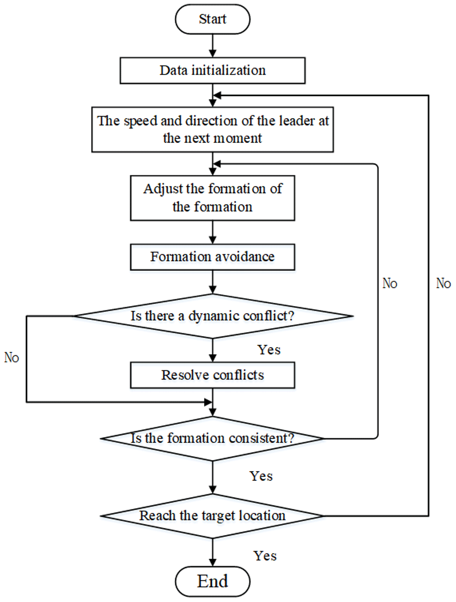
The specific implementation steps are as follows.Step 1: data initialization, mainly to initialize the number of formation robots, the initial positions of robots, the initial speeds of robots, the destination of the formation leader, the position error of the followers and the leader, and the communication topology of the formation.Step 2: according to Eq. (6), calculate the speed of the leader at the next moment.Step 3: adjust the formation according to Eq. (9) to make the formation reach a consensus.Step 4: according to Eqs. (8) and (10), make the leader and follower formation's complete obstacle avoidance.Step 5: judge whether there is a dynamic conflict between the robots. If there is a conflict, use Eq. (17) to resolve the conflict.Step 6: if the formation reaches the destination, the algorithm ends and the path is output. Otherwise, turn to step (2).

4 Numerical simulation and result analysis

4.1 Experimental structure and data initialization

The experimental simulations were conducted using (The MathWorks Inc., 2019) as the simulation software on a workstation running the Windows 10 operating system. The workstation is equipped with an Intel(R) Core(TM) i9-12900F CPU running at 3.2 GHz and 32.0 GB of RAM along with a GeForce NVIDIA RTX 3090TI GPU with 24 GB of memory. The simulations were performed in a virtual environment with dimensions of 30 × 30 m² representing an indoor space. The robot formation consisted of multiple robots, all of which were of the same type and equipped with basic navigation, obstacle avoidance, communication, and other necessary functions. One robot was designated the leader with the remaining robots acting as followers, following the leader's trajectory while maintaining appropriate spacing and avoiding obstacles.

In a static environment, the coordinates of the obstacles are set randomly. The obstacles are not updated during the experiment after being randomly generated to compare movement outcomes from different robot formations, as illustrated in Fig. 4a. In the dynamic obstacle environment, the static obstacle position remains unchanged, which increases the robot's obstacle.

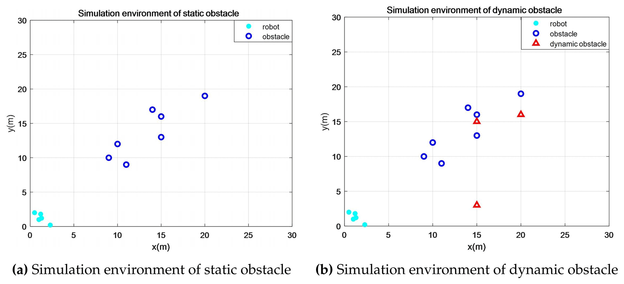
Figure 4 Schematic simulation environment construction: the light-blue dots are robots, the black dots are static obstacles, and the red triangles are dynamic obstacles.

The starting positions, desired positions, and speeds of dynamic obstacle robots are initialized randomly and kept constant with the number of formation robots after initialization, as shown in Fig. 4b.

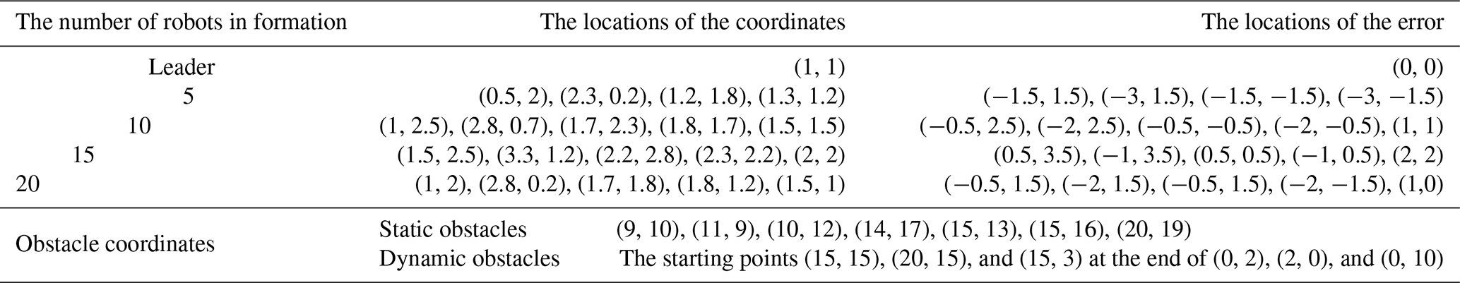
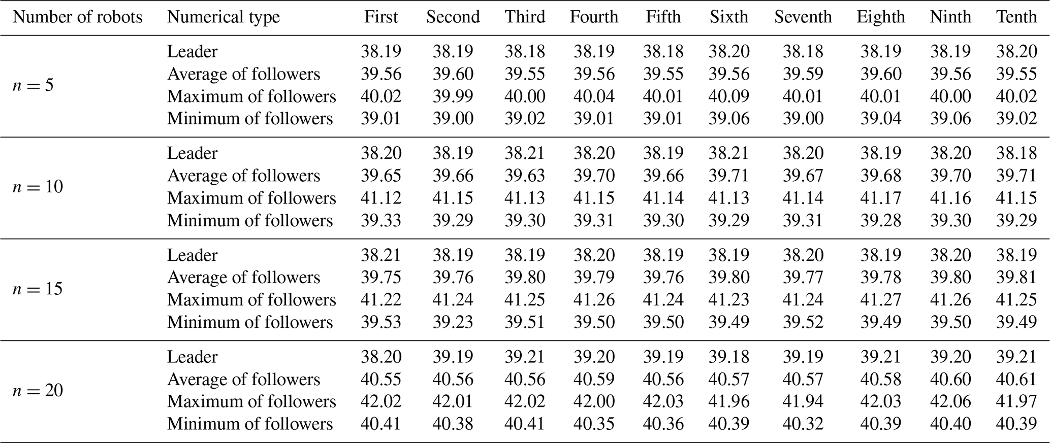
The number of robots in different formations is $n=[\mathrm{5},\mathrm{10},\mathrm{15},\mathrm{20}]$. According to the different environments, the initial position $\left(p_i^x\left(\mathrm{0}\right),p_i^y\left(\mathrm{0}\right)\right)$, static obstacle position $\left(p_{\mathrm{obs}}^x,p_{\mathrm{obs}}^y\right)$, and dynamic obstacle initial position $\left(p_{c_k}^x\left(\mathrm{0}\right),p_{c_k}^y\left(\mathrm{0}\right)\right)$ are randomly obtained for initialization. The data initialization results are shown in Table 1. In Table 1, the simulation experiment assumes that there is one leader in each formation, and the follower i, $i=[\mathrm{1},\mathrm{19}]$ represents the number of followers.

Table 1 Parameter initialization table in different experimental environments.

4.2 Experimental results and analysis

In this section, the MRF is tested in a static and dynamic obstacle simulation environment, and the experimental results are analyzed.

4.2.1 Static obstacle environment

To prove that the method of the MRF is universal, the number of formation robots is increased when the obstacle environment remains unchanged. Ten experiments were carried out on the formations of 5, 10, 15, and 20 robots, and the results were analyzed. Figure 5 depicted the experimental results without improving the model. The static obstacle avoidance and consistent formation methods based on spring force are integrated into the static obstacle environment. Figure 5 represents the formation trajectory, the position deviation error among the followers and the leader, and the error among the actual position and the ideal position of each robot, respectively.

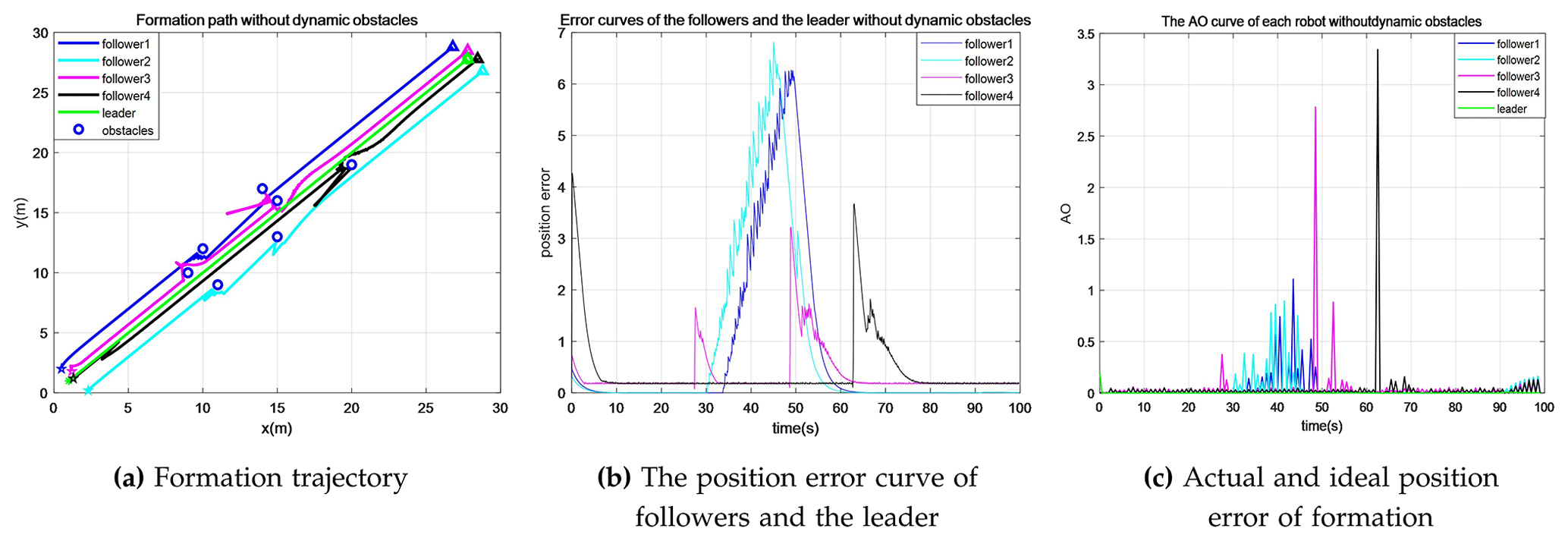
Figure 5 There is no experimental result when the model is formed to avoid obstacles. The model only directly uses methods such as static obstacle avoidance based on spring force (Zhao et al., 2020) and consistent formation (Pan et al., 2019); n=5.

(1) Analysis of the trajectory of the formation

We observe the trajectory of each robot in Fig. 5a. Except for the leader's trajectory, the path of the followers is erroneous; more specifically, when the simulation time is 29 s, the position error for the three followers is large. Because the virtual spring force increases when moving to the obstacle position, which decreases the motion space, the conflict resolution algorithm is not added. Moreover, there is no speed limit, which makes the followers deviate from the formation seriously. The improved model is used to carry out experiments in the same environment with 5-, 10-, 15-, and 20-robot formation motion trajectories to address the aforementioned issues. The experimental results, depicted in Fig. 6, show that the robots' motion trajectories are relatively smooth. We can find that the improved trajectory has the following characteristics: by comparing them with Fig. 5a and Fig. 6a, the trajectory of the followers has been significantly improved by the improved algorithm. After 25–30 s of disturbance by obstacles, follower 2 picks a path that diverges from the leader, but the constraint of consistency limits the departure. Simultaneously, the formation is constrained by the maximum velocity function, reducing the probability of deviating from the intended direction. The trajectory diagram demonstrates that there is no significant position error in the followers and that they may swiftly rejoin the formation after passing through the obstacle region, particularly when the formation of five robots crosses the (20, 19) obstacle.

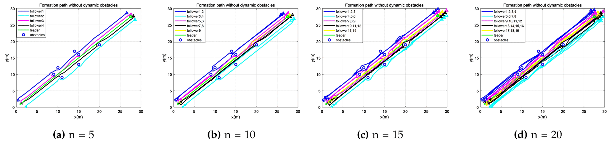
Figure 6 Formation trajectory of the improved model in the static obstacle environment. The robots in the formation are n=5, n=10, n=15, and n=20.

When the number of robots in the formation increases, the leader's path remains constant, and then the followers form several relatively unified paths. Robots with similar trajectories used the same path color in Fig. 6. As the number of robots increases, the dynamic conflict resolution algorithm is implemented to force followers to collaborate and avoid stagnation or significant position divergence caused by mutual avoidance. We observed the trajectories of follower 1 and follower 2 in Fig. 6b. When the first obstacle is encountered, follower 1 decelerates as a result of the collision between the two robots on the path. The resolution algorithm guides the two robots to choose both sides of the obstacle to move. When the two robots encountered obstacles for the second time, there was a significant space between them in the passing time without path conflict. If the paths overlap, then both choose the shortest path to cross between the two obstacles. When Fig. 6c and d are compared, the paths of robots in similar positions are unified with no obstacles in the trajectory. According to the initial position, the conflict resolution between follower 1 and follower 2 in Fig. 6b occurs when the first obstacle is encountered and a unified branch path is formed. When the robots in the branch path encounter a conflict, it will disperse movement. There is no stagnation phenomenon when robots are in conflict. At the same time, with the increase in the number of robots, the formation consistency and speed limit model of robots' trajectories are proposed to ensure that there is no significant deviation, especially to decongest and block the phenomenon.

(2) Position error between the leader and followers

When Fig. 5b and Fig. 7a are compared, it can be seen from Fig. 5b that the error associated with the leader path is large and is estimated as 11.3. This is due to the deviation of the followers from the formation. After implementing the improved algorithm, the maximum value of the error does not exceed 39 % of the maximum error in Fig. 5b regardless of the number of robots in the formation. The time of the first maximum position error of the followers and the leader is between 27 and 40 s. Since the speed does not limit the formation, the time to reach the obstacle area is earlier, and the maximum position error in Fig. 6b occurs earlier. The maximum error value in Fig. 7a is reduced to 2.3 after the consistent speed formation is restricted, which is 20.3 % of the original value. At the same time, the experimental results show that the follower can get closer to the ideal position after determining the digraph. All the results were shown by the characteristics of trajectory convergence. After crossing the obstacle area, the error peak point appears at 40 s, and then the position error decreases. However, the error value in Fig. 5b fluctuates obviously. The convergence of the position error value of the improved algorithm presents a monotonic trend and has minimal fluctuation.

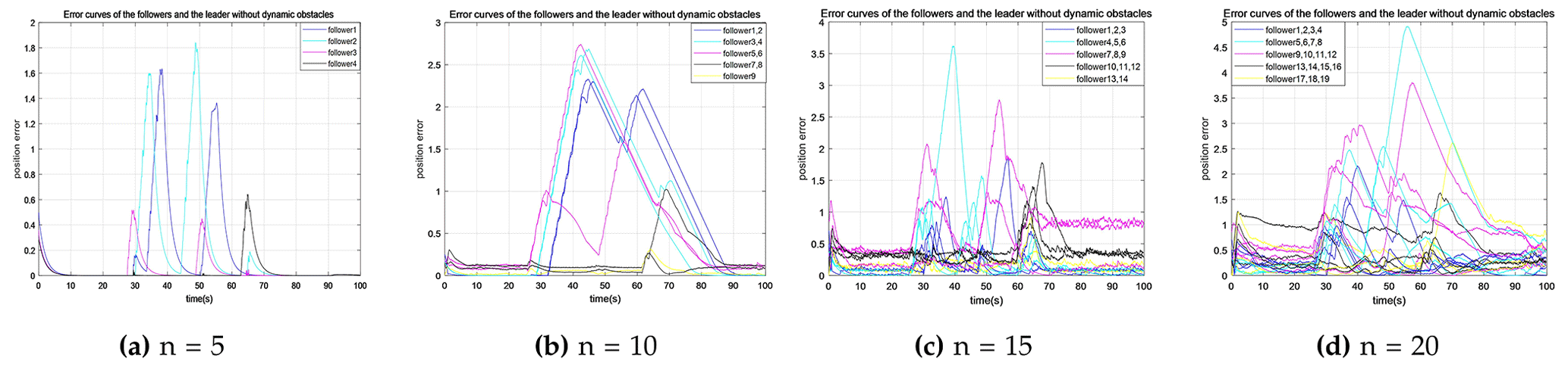
Figure 7 The position error of the leader and followers of the improved model formation movement in the static obstacle environment. The robots in the formation are n=5, n=10, n=15, and n=20.

In Fig. 7, as the number of formation robots increases, the position error among the followers and the leader increases. For the five-robot formation, the maximum error among the followers and the leader occurs in 36.7 s, and the error value is 2.3. The maximum error of 10 robots is 42.3 s, and the error value is 2.76, which is 18.5 % higher than that of 5 robots. The maximum error of 15 robots occurred in 39.7 s, and the error value is 3.67, which is 24.79 % higher than that of 10-robot formations. The maximum error of 20 robots is 55.1 s, and the error value is 4.85, which is 24.33 % higher than that of 15-robot formations. The maximum error time increases with the number of formation robots. The increased distance error is due to a plane envelope in the optimal path or a branch of the optimal path with infinite space under the consistency constraint. When the number of robots increases, the speed of individual robots at the cost of expanding the path envelope under speed control is maintained, and the expansion of the path envelope inevitably increases the position error. Combined with the positions of static obstacles in Fig. 6 and the position error curves of each robot in Fig. 7, we can find that the occurrences of position obstacles with peak values correspond to each other. However, the improved algorithm enables the robot to obtain good control. The monotonic increase and decrease in the error curve indicate that the formation robots have achieved good cooperative control. The conflict resolution algorithm effectively eliminates the mutual disturbance in the formation of robots. Although there is slight fluctuation in the trajectory diagram of the robot error curve after the 90 s in Fig. 7a and b, it is evident that the position error fluctuation of 15 robots and 20 robots in formation occurs when the robots reach the ideal position since the deceleration process of the robots in the front will affect the robots in the rear. The influence will increase with the increased number of robots.

Analyzing the data in Table 2 reveals that the path length has little effect on the leader in the formation. The fluctuation value is less than 2.7 %, which indicates that the stability of the leader in a different number of formations meets the control requirements. The average of the maximum and minimum values of the followers' path length is less than 5 % and signifies good stability in the formation movement period. The movement path of the robots is controlled in an acceptable range. This increased value is monotonically increasing. Therefore, it can be predicted that there will be a bottleneck in the number of formation robots in the limited path area.

Table 2 The path lengths of 10 experiments without dynamic obstacles. The experiments were under the condition of the number of robots in different formations.

4.2.2 Dynamic obstacle environment

(1) Analysis of the trajectory of the formation

In a static obstacle environment, dynamic obstacle robots were added to dynamic obstacle avoidance experiments. First, the static obstacle avoidance method based on spring force and the consistent formation method is used in the dynamic environment, as shown in Fig. 8. Figure 8a represents the three-dimensional formation motion trajectory. The static obstacles do not change with time even if the time axis is added to the trajectory diagram, as shown in the blue cylinder. Figure 8b is the projection of Fig. 8a in the x–y plane, which can directly show the two-dimensional motion trajectory of each robot. Figure 8c represents the position deviation error between the followers and the leader. Figure 8d shows the error between the actual and ideal positions of each robot.

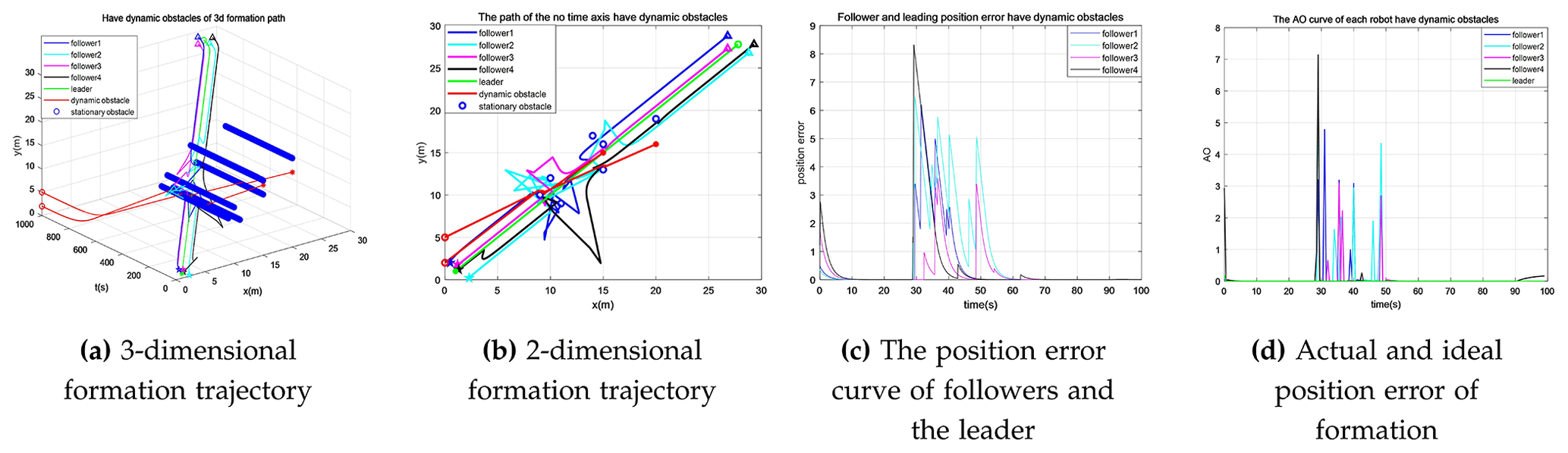
Figure 8 Curve of the experimental results when there are dynamic obstacles and no speed limit robots n=5.

To verify the effectiveness of the improved model in a dynamic obstacle environment, our proposed method comprised the formation of 5, 10, 15, and 20 robots in carrying out the experiment of the motion trajectory, as shown in Fig. 9. The trajectory of the robot in Fig. 9 is relatively smooth, with no serious deviation of the robots from the formation. When the trajectories of each robot in Figs. 8a and 9a are compared, it is clear from Fig. 9a that the trajectory has a significant improvement of the followers. Following an improved algorithm of the formation-encountering obstacles, the followers achieved the lowest deviation from the leader. After obstacle avoidance is completed, the followers quickly reach consistency with the leader until the endpoint.

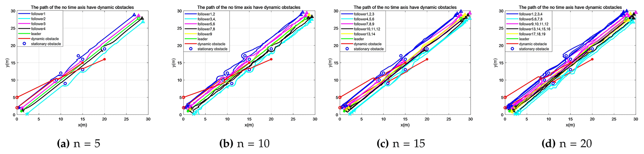
Figure 9 The trajectory diagram of the improved model formation in a dynamic obstacle environment. The robots in the formation are n=5, n=10, n=15, and n=20.

The path pattern obtained in Fig. 9 is smoother than the path obtained in Fig. 6 due to the dynamic conflict resolution algorithm that provides obstacle avoidance speed. The time and space conflict path movements of the robot formation are well planned. However, after comparing all the route formations without dynamic obstacles, a slight fluctuation causes interference in the formation, as shown in Fig. 9. As the number of formation robots increases, the robots form regular paths of formation movement. The number of fixed paths is different from Fig. 9c and d.

When the number of robots is 15, the robots can run in three optimal trajectories through the time difference. When the number of robots increases to 20, the adjustment of the time difference is limited, and it can be seen that there are four main trajectories, which is indicated by the fact that the trajectory parameter information can interact with itself. By carefully observing the trajectory of each robot, it can be found that, except for the disturbance caused by dynamic obstacles, the motion characteristics of the individual robot are similar to those of a static environment, which will not be repeated here.

(2) Position error between the leader and followers

Compared with Figs. 8c and 10a, both of them show the position error diagram of the leader and followers of a five-robot formation, and the maximum deviation error of the followers in Fig. 8c is 8.3. In the improved model, even if the number of formation robots is 20, the maximum error is less than 7. In Fig. 8c, the position error of the followers is large and consequently increases the error fluctuation due to the great influence of obstacles on formation motion. In Fig. 10a, the position error is small and evenly distributed with each robot reaching the peak error twice, which shows that the improved algorithm ensures the stability of the robot's motion.

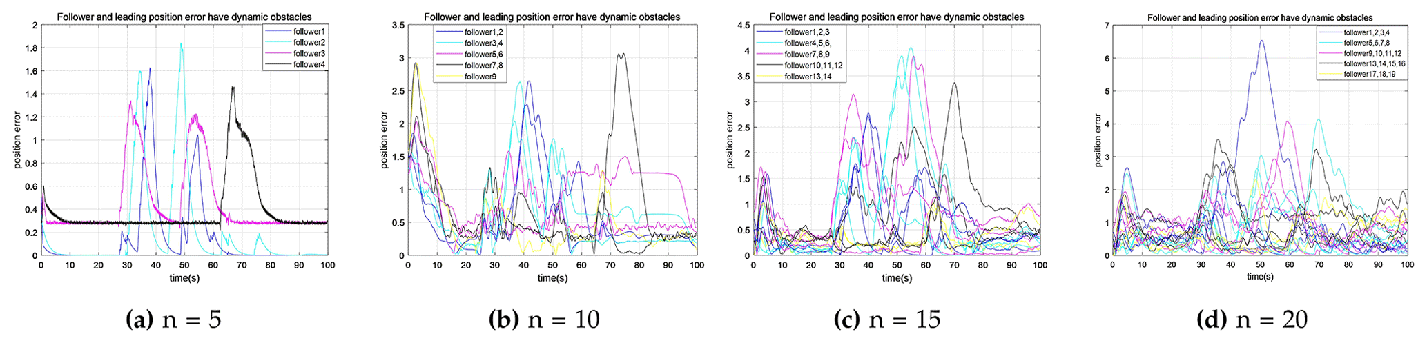
Figure 10 The position error of the leader and followers of the improved model formation movement in an environment with dynamic obstacles. The robots in the formation are n=5, n=10, n=15, and n=20.

From Figs. 10a and 7a, the error waveforms due to rising and falling trends of followers are almost the same when compared, but it is evident that the error increases, especially for follower 4 and follower 3. The reference value of the error difference for follower 4 is 0.27 higher than that of follower 3, as depicted in Fig. 7a. By observing the positions of the two robots, it can be found that their followers are both in front of the leader's direction of motion with the possibility of conflict in the presence of dynamic obstacles during the movement. Therefore, the two robots should leave space for the leader's movement and avoid conflict with dynamic obstacles. Hence, the overall path error is relatively large, which increases by 66.23 % and 52.34 % compared with the error in the static obstacle environment in the absence of the dynamic obstacles for followers 4 and 3, respectively. The results presented in Fig. 10 show the characteristics of trajectory convergence. The peak value of the follower's position error decreases in avoiding static and dynamic obstacles. Simultaneously, it can be found that, when the robot reaches the target point, the error value increases for the second time, precisely when the number of robots increases. Therefore, when the robot moves to the desired position, the position error tends to increase, which is consistent with the motion characteristics of the static obstacle environment.

(3) Error analysis for ideal and real environments

There is a significant improvement in the robot's actual and ideal position errors in Fig. 11a compared to Fig. 8d, except for the peak time error and initial time. The error due to follower 4 is large in Fig. 8d compared to the results obtained in Fig. 10a, which has a maximum value of 0.17. When follower 3 is compared in Figs. 8d and 10a, the error from Fig. 8d is reduced by 98.6 % at 29.8 s. The maximum error of follower 1 at 31.5 s is reduced by 95.78 % compared to before the implementation of the improved algorithm. At the same time, it can be seen from the experimental results that, after the determination of the directed graph, the followers move closer to the ideal position. In Fig. 11a, the position error decreases after passing through all the obstacles for 23 s. After reaching stability, the formation keeps almost zero errors and drives to the desired position. At 67 s, there is an obstacle in front of follower 4, which increases the error. However, the error decreases when follower 4 returns to the formation position.

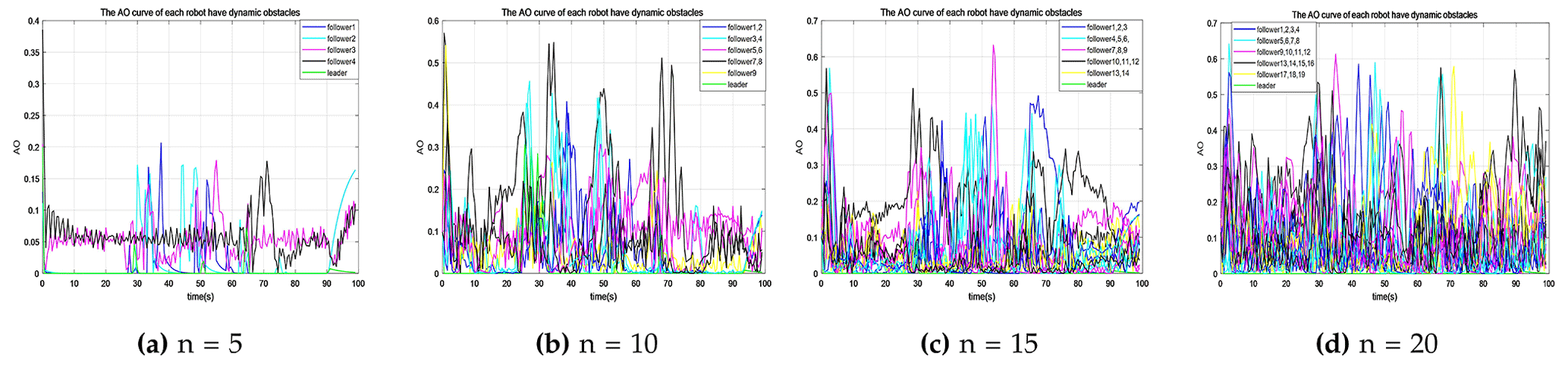
Figure 11 The error between the ideal state and the actual position of the formation move of the improved model in an environment with dynamic obstacles. The robots in the formation are n=5, n=10, n=15, and n=20.

Let us analyze the data presented in Table 3. They show that the total path lengths of 10-, 15-, and 20-robot formations are 2.05, 3.18, and 4.27 times those of 5 robots. In the presence of dynamic obstacles, the total growth rate for the formation path length is greater than that of the static environment with the increase in the number of robots. However, the number of robots in the formation of the conflict increases exponentially. The total path length of the formation has a polynomial increment, which indicates the practicability and adaptability of the formation system. To determine the stability of the formation in dynamic obstacle avoidance, the path length data of the robots after 10 simulations are statistically analyzed. The results are shown in Table 4.

Table 3 Comparison of path length in an environment with dynamic obstacles.

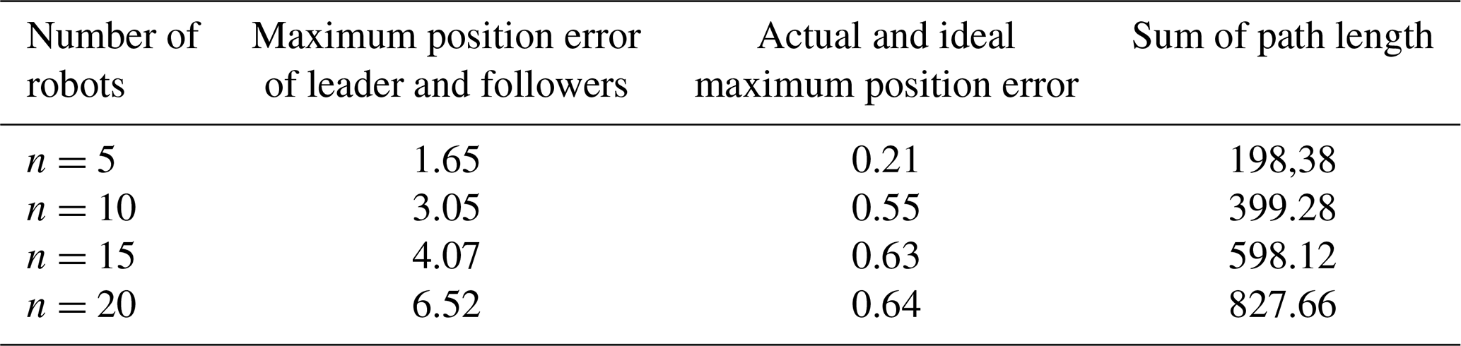
Table 4 Path length of formation movement in a dynamic obstacle environment.

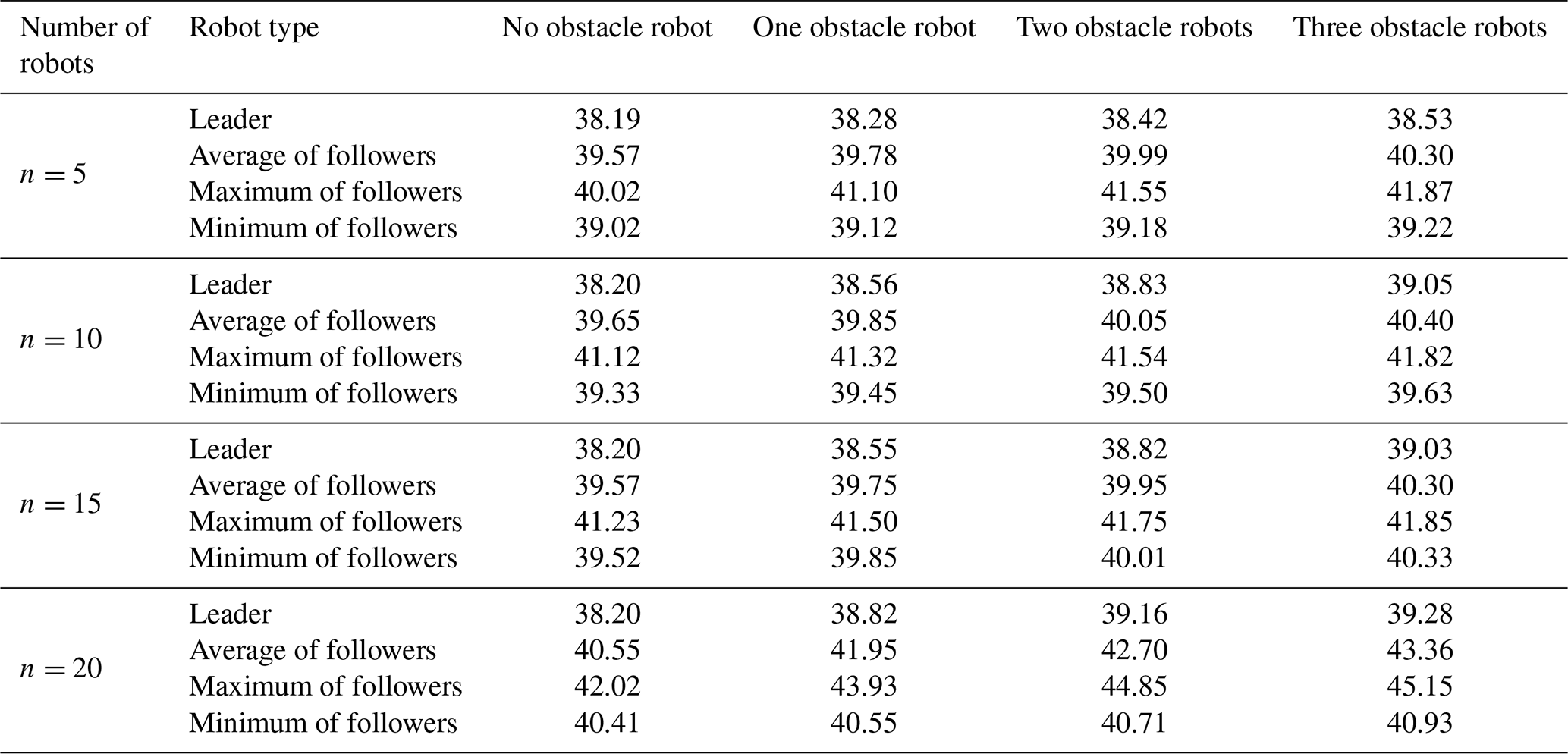
Moreover, Table 4 shows that when the number of dynamic obstacles increases, the average, maximum, and minimum path lengths of a leader and its followers increase by no more than 1.6 %, reflecting the adaptability of the system to dynamic obstacles. When the number of dynamic obstacles is the same, the leader's path length increases by no more than 3.22 % with the increase in the number of formation robots. Similarly, if the number of formation robots is between 5 and 10 robots, then the average path length of the followers increases by 2.19 %. Moreover, Table 4 shows that when the number of dynamic obstacles increases, the average, maximum, and minimum path lengths of a leader and its followers increase by no more than 1.6 %, reflecting the adaptability of the system to dynamic obstacles. When the number of dynamic obstacles is the same, the leader's path length increases by no more than 3.22 % with the increase in the number of formation robots.

Similarly, if the number of formation robots is between 5 and 10 robots, between 10 and 15 robots, and between 15 and 20 robots, then the average path length of the followers increases by 2.19 %, 3.97 %, and 5 %, respectively. The maximum path length and minimum path length of the followers increase by no more than 5 % with the increase in the number of robots. The path length increases more when the number of formation robots increases than when there are no dynamic obstacles. Therefore, this shows the stability of the system in a static and dynamic obstacle environment. However, there is an upper limit on the number of dynamic obstacles and formation robots in the limited space.

5 Conclusions

We examined the effect of an increasing number of robots on formation operations, with an emphasis on the constrained space environment. Based on previous studies, a static obstacle avoidance model based on spring force mapping is proposed. Due to the mutual disturbance produced by the growing number of robots, the VO algorithm has been improved to resolve robot collisions during the dynamic mobility process. The leader is added to the formation. The dynamic speed limit function based on position error is established to ensure the formation consistency between the followers and the leader. Simultaneously, the leader can share the obstacle avoidance information with obstacle avoidance speed, the task completion speed of the formation is improved, and the motion efficiency of the robots is improved. The simulation results indicate that the improved obstacle avoidance method can provide more precise guidance for formation robots. Meanwhile, as the number of robots increases, the position error and average path length do not significantly increase, indicating that the proposed method applies to a large number of multi-robot formation obstacle avoidances.