Improved strategies of the Equality Set Projection (ESP) algorithm for computing polytope projection

​​​​​​​This paper proposes an optimization method for the Equality Set Projection algorithm to compute the orthogonal projection of polytopes. However, its computational burden significantly increases for the case of dual degeneracy, which limits the application of the algorithm. Two improvements have been proposed to solve this problem for the Equality Set Projection algorithm: first, a new criterion that does not require a discussion of the uniqueness of the solution in linear programming, which simplifies the algorithm process and reduces the computational cost; and second, an improved method that abandons the calculation of a ridge's equality set to reduce the computational burden in the case of high-dimensional dual degeneracy.

1 Introduction

Orthogonal projection is valuable for both theoretical research (Kwan et al., 2022; Xu and Guo, 2021) and engineering applications (Xia et al., 2021; Liu et al., 2023), particularly as a basic operator for polytopes, which are a type of geometric structure composed of flat boundaries and giving a good representation of linear constraints on variables. The orthogonal projection of polytopes is extensively applied in the field of control and optimization (Borrelli et al., 2017; Lee and Kouvaritakis, 2000; Sadeghzadeh, 2018). For example, the calculations of the Minkowski sum (Teissandier and Delos, 2011), controllable set (Vincent and Wu, 1990), reachable set (Rakovic et al., 2006), and parametric linear program (Jones et al., 2008) can all be transformed into the projection of polytopes.

Traditional projection algorithms can be grouped into three classes, i.e., Fourier elimination (Keerthi and Sridharan, 1990; Saraswat and Hentenryck, 1995), block elimination (Balas, 1998; Fukuda and Prodon, 1996), and vertex enumeration (Avis, 1998). The former two algorithms require expensive computation and produce a lot of redundant inequalities. The third algorithm is suitable for polytopes with fewer vertices; however, the number of vertices of a high-dimensional polytope exceeds the number of half-spaces. Thus, it is not an efficient algorithm for the high-dimensional cases.

The Equality Set Projection (ESP) algorithm was proposed in Jones et al. (2004), and it applies the inspiration of the gift-wrapping algorithm to the projection calculation. Under the condition of non-degeneracy, the complexity of ESP is linear in the number of half-spaces, which offers a tremendous advantage compared to the traditional projection algorithms. However, in the case of dual degeneracy, the computation grows exponentially.

Dual degeneracy is a frequently encountered phenomenon in control applications. For instance, when variables have constant maximum and minimum constraints, the occurrence of dual degeneracy is more likely. Unfortunately, this limitation curtails the wider application of ESP algorithms in the control field. Therefore, the primary motivation behind enhancing the ESP method is to improve its performance under dual-degeneracy conditions. We propose a novel criterion based on the non-zero rows of the null-space matrix to address the issue of discussing the uniqueness of solutions under such conditions. Furthermore, we introduce an improved strategy that eliminates the need to search for equation sets under dual-degeneracy conditions. These two advancements render the ESP algorithm more concise, efficient, and easily implementable. Consequently, the algorithm's performance in the situations involving dual degeneracy has been significantly enhanced, which paves the way for further promotion and application of ESP in engineering practices.

The paper is organized as follows. The preliminary knowledge and the workflow of the original ESP algorithm are introduced in Sect. 2. The two proposed improvement strategies are given in Sects. 3 and 4. Numerical simulation comparisons between the original ESP and the improved ESP are reported in Sect. 5, and final conclusions given in Sect. 6.

2 Preliminaries and existing results

2.1 Definitions and notation

• 1.

  A polytope is a bounded polyhedron defined by the intersection of closed half-spaces. Let P equal $\left\{(\mathit{x},\mathit{y})\in R^d\times R^k|\mathbf{C}\mathit{x}+\mathbf{D}\mathit{y}\le \mathit{b}\right\}$; the orthogonal projection of P onto x space is defined as

  $${\mathit{\pi }}_d\left(P\right)=\left\{\mathit{x}\in R^d|\exists \mathit{y}\in R^k,(\mathit{x},\mathit{y})\in P\right\}.$$
• 2.

  f is a face of the polytope $P\subset R^d\times R^k$ if there exists a hyperplane $\left\{(\mathit{x},\mathit{y})\left|{\mathit{c}}^{\mathrm{T}}\mathit{x}+{\mathit{d}}^{\mathrm{T}}\mathit{y}=b\right.\right\}$, where c∈R^d, d∈R^k, and b∈R such that

  $$f=P\cap \left\{(\mathit{x},\mathit{y})\in R^d\times R^k|{\mathit{c}}^{\mathrm{T}}\mathit{x}+{\mathit{d}}^{\mathrm{T}}\mathit{y}=b\right\}$$

  and ${\mathit{c}}^{\mathrm{T}}\mathit{x}+{\mathit{d}}^{\mathrm{T}}\mathit{y}\le b$ for all $(\mathit{x},\mathit{y})\in P$. The face of the polytope $P\subset R^d\times R^k$ refers to the face of dimension n−1, whereas the ridge refers to the face of dimension n−2.

• 3.

  The affine hull of every face of the polytope is

  $$\text{aff}f=\left\{(\mathit{x},\mathit{y})\in R^d\times R^k|{\mathit{c}}^{\mathrm{T}}\mathit{x}+{\mathit{d}}^{\mathrm{T}}\mathit{y}=b\right\}.$$
• 4.

  If A is a matrix and $E\subseteq \left\{\mathrm{1},\mathrm{\dots },q\right\}$, then A_E is a matrix formed by rows of A whose indices are in E. If P is a polytope, then the notation P_E refers to the set $P_E=P\cap \left\{z\left|{\mathbf{C}}_E\mathit{x}+{\mathbf{D}}_E\mathit{y}=b_E\right.\right\}$.

• 5.

  E is an equality set of P if and only if E=G(E), where

  $$G\left(E\right)=\left\{i\in \left\{\mathrm{1},\mathrm{\dots },q\right\}|{\mathbf{C}}_i\mathit{x}+{\mathbf{D}}_i\mathit{y}=b_i,\forall (\mathit{x},\mathit{y})\in P_E\right\}.$$
• 6.

  N(A) is defined as a matrix whose columns form an orthonormal basis for the null space of A.

2.2 Auxiliary results

The following results can be found in Jones (2005), Ziegler (1995), Webster (1994), and Balas and Oosten (1998), respectively. Their proofs are omitted for the sake of brevity.

Theorem 2.1 (Jones, 2005) Given a polytope

$$P=\left\{(\mathit{x},\mathit{y})\in R^d\times R^k|\mathbf{C}\mathit{x}+\mathbf{D}\mathit{y}\le \mathit{b}\right\},$$

if E is an equality set of P, then P_E is a face of P. Furthermore, if F is a face of P, then there exists a unique equality set such that F=P_E.

Proposition 2.1 (Ziegler, 1995) If $P\subset R^d\times R^k$ is a polytope, then the projection of P onto R^d is a polytope.

Proposition 2.2 (Webster, 1994) If $F_{\mathrm{1}},\mathrm{\dots },F_t$ are facets of a polytope $P=\left\{\mathit{z}\in R^n|A\mathit{z}\le \mathit{b}\right\}$, $\text{aff}{F}_i=\left\{\mathit{z}\in R^n|{\mathit{a}}_i^{\mathrm{T}}\mathit{z}=b_i\right\}$, where each a_i∈Rⁿ, b_i∈R, then

$$P=\text{aff}P\cap \left\{\mathit{x}\in R^n\left|\left[\begin{array}{c}{\mathit{a}}_{\mathrm{1}}^{\mathrm{T}}\\ \mathrm{⋮}\\ {\mathit{a}}_t^{\mathrm{T}}\end{array}\right]\mathit{x}\le \left[\begin{array}{c}{b}_{\mathrm{1}}\\ \mathrm{⋮}\\ b_t\end{array}\right]\right.\right\}.$$

Proposition 2.3 (Ziegler, 1995) If $P\subset R^d\times R^k$ is a polytope, then for every face F of π_d(P), the pre-image ${\mathit{\pi }}_d^{-\mathrm{1}}\left(F\right)$ is a face of P.

Proposition 2.4 (Jones, 2005) If $M=\left\{(\mathit{x},\mathit{y})\in R^d\times R^k|{\mathbf{C}}_E\mathit{x}+{\mathbf{D}}_E\mathit{y}=b_E\right\}$ is a affine set, then the projection of M onto R^d is

$${\mathit{\pi }}_d\left(M\right)=\left\{\mathit{x}\in R^d\left|\mathbf{N}{\left({\mathbf{D}}_E^{\mathrm{T}}\right)}^{\mathrm{T}}{\mathbf{C}}_E\mathit{x}=\mathbf{N}{\left({\mathbf{D}}_E^{\mathrm{T}}\right)}^{\mathrm{T}}{b}_E\right.\right\}.$$

Proposition 2.5 (Balas and Oosten, 1998) If E is an equality set of polytope

$$P=\left\{(\mathit{x},\mathit{y})\in R^d\times R^k|\mathbf{C}\mathit{x}+\mathbf{D}\mathit{y}\le \mathit{b}\right\},$$

then $\text{dim}{\mathit{\pi }}_d\left(P_E\right)=\text{dim}{P}_E-k+\text{rank}{\mathbf{D}}_E$.

2.3 Original ESP algorithm

We introduce the workflow of the original ESP algorithm in this subsection. A brief introduction is given here, and the details can be found in Jones (2005).

The algorithm is initialized by discovering a random facet F_π in π_d(P). Then we compute all ridges contained in the initial facet and search all facets adjacent to it through each ridge. Subsequently, we compute all the ridges of each new facet and let the iterating process continue until all the ridges appear twice. According to the property of the polytope, each ridge exactly connects to two facets. Therefore, all facets of π_d(P) can be found by this iteration. From Proposition 2.2, we finally get ${\mathit{\pi }}_d\left(P\right)=\left\{\mathit{x}\in R^d\left|\mathbf{G}\mathit{x}\le \mathit{g}\right.\right\}$.

The ESP algorithm consists of three key oracles as given below. Shooting Oracle:

$$\left(E_{f_{\mathrm{0}}},{\mathit{a}}_f,b_f\right)=\text{SHOOT}\left(P\right).$$

Ridge Oracle:

$$L{E}_r=\text{RDG}\left(E_f,{\mathit{a}}_f,b_f\right).$$

Adjacency Oracle:

$$\left(E_{\mathrm{adj}},{\mathit{a}}_{\mathrm{adj}},b_{\mathrm{adj}}\right)=\text{ADJ}\left(\left(E_f,{\mathit{a}}_f,b_f\right)\left(E_r,{\mathit{a}}_r,b_r\right)\right).$$

The SHOOT oracle randomly obtains an equality set $E_{f_{\mathrm{0}}}$ of P satisfying ${\mathit{\pi }}_d\left(P_{E_{f_{\mathrm{0}}}}\right)=\left\{\mathit{x}|{\mathit{a}}_f^{\mathrm{T}}\mathit{x}=b_f\right\}\cap {\mathit{\pi }}_d\left(P\right)$ as a facet of π_d(P), the RDG oracle returns all ridges contained in the facet $\left(E_f,{\mathit{a}}_f,b_f\right)$ of π_d(P), and the ADJ oracle takes two equality sets E_r and E_f of P and returns the unique equality set E_adj, where ${\mathit{\pi }}_d\left(P_{E_f}\right)=\left\{\mathit{x}|{\mathit{a}}_f^{\mathrm{T}}\mathit{x}=b_f\right\}\cap {\mathit{\pi }}_d\left(P\right)$ is a facet of π_d(P) and ${\mathit{\pi }}_d\left(P_{E_r}\right)=\left\{\mathit{x}|{\mathit{a}}_r^{\mathrm{T}}\mathit{x}=b_r\right\}\cap {\mathit{\pi }}_d\left(P_{E_f}\right)$ is a ridge of π_d(P) with ${\mathit{\pi }}_d\left(P_{E_r}\right)\subset {\mathit{\pi }}_d\left(P_{E_f}\right)$.

2.3.1 Outline of the ESP algorithm

Step 1. Get an initial facet $\left(E_{f_{\mathrm{0}}},{\mathit{a}}_f,b_f\right)$ of P: $\left(E_{f_{\mathrm{0}}},{\mathit{a}}_f,b_f\right)=\text{SHOOT}\left(P\right)$. Then, all the ridges contained in the facet are calculated: $L{E}_r=\text{RDG}\left(E_{f_{\mathrm{0}}},{\mathit{a}}_f,b_f\right)$. For each element $\left(E_{r_j},a_{r_j},b_{r_j}\right)$ in LE_r, record $\left(\left(E_{f\mathrm{0}},{\mathit{a}}_{f\mathrm{0}},b_{f\mathrm{0}}\right),\left(E_{r_j},a_{r_j},b_{r_j}\right)\right)$ in list L and let $\mathbf{G}={\mathit{a}}_f^{\mathrm{T}}$, g=b_f.

Step 2. If L≠ϕ, select an element $\left(\left(E_{f_i},a_{f_i},b_{f_i}\right),\left(E_{r_i},a_{r_i},b_{r_i}\right)\right)$ randomly from list L and let $\left(\left(E_{\mathrm{fn}},a_{\mathrm{fn}},b_{\mathrm{fn}}\right),\left(E_{\mathrm{rn}},a_{\mathrm{rn}},b_{\mathrm{rn}}\right)\right)=\left(\left(E_{f_i},a_{f_i},b_{f_i}\right),\left(E_{r_i},a_{r_i},b_{r_i}\right)\right)$. If L=ϕ, stop and report G and g.

Step 3. Search the adjacent facet such that $\left(E_{\mathrm{adj}},{\mathit{a}}_{\mathrm{adj}},b_{\mathrm{adj}}\right)=\text{ADJ}\left(\left(E_{\mathrm{fn}},a_{\mathrm{fn}},b_{\mathrm{fn}}\right),\left(E_{\mathrm{rn}},a_{\mathrm{rn}},b_{\mathrm{rn}}\right)\right)$ and let

$$\mathbf{G}=\left[\begin{array}{c}\mathbf{G}\\ {\mathit{a}}_{\mathrm{adj}}^{\mathrm{T}}\end{array}\right],\mathit{a}=\left[\begin{array}{c}\mathit{a}\\ b_{\mathrm{adj}}\end{array}\right].$$

Then, all the ridges contained in the adjacent facet can be calculated: $L{E}_r=\text{RDG}\left(E_{\mathrm{adj}},{\mathit{a}}_{\mathrm{adj}},b_{\mathrm{adj}}\right)$. For each element $\left(E_{r_j},a_{r_j},b_{r_j}\right)$ in LE_r, if there exists an element in L that already contains $E_{r_j}$, we remove the element from the list. Otherwise, we add element $\left(\left(E_{r_j},a_{r_j},b_{r_j}\right),\left(E_{\mathrm{adj}},{\mathit{a}}_{\mathrm{adj}},b_{\mathrm{adj}}\right)\right)$ to list L. Go to Step 2.

2.3.2 SHOOT oracle

Step 1 (selecting a direction γ and finding a point on the surface of P)

Randomly choose γ∈R^d and solve the following linear programming.

$$\begin{array}{}\text{(1)}& \begin{array}{l}\left(r^{*},{\mathit{y}}^{*}\right)=\underset{(r,\mathit{y})\in R\times R^k}{\arg max}r,\\ \text{s.t.}\mathbf{C}\mathit{\gamma }r+\mathbf{D}\mathit{y}\le \mathit{b}\end{array}\end{array}$$

Step 2 (determining whether a facet of π_d(P) is found)

Get $E_{f_{\mathrm{0}}}$ as $E_{f_{\mathrm{0}}}=\left\{i|{\mathbf{C}}_i\mathit{\gamma }r+{\mathbf{D}}_i\mathit{y}=b_i\right\}$. If $\text{Rank}\left(\mathbf{N}{\left({\mathbf{D}}_{E_{f_{\mathrm{0}}}}^{\mathrm{T}}\right)}^{\mathrm{T}}{\mathbf{C}}_{E_{f_{\mathrm{0}}}}\right)=\mathrm{1}$, go to Step 3. Otherwise, go to Step 1.

Step 3 (computing the affine hull of the facet and normalizing)

$$\begin{array}{l}\left[{\mathit{a}}_f^{\mathrm{T}},b_f\right]=\mathbf{N}{\left({\mathbf{D}}_{E_{f_{\mathrm{0}}}}^{\mathrm{T}}\right)}^{\mathrm{T}}\left[{\mathbf{C}}_{E_{f_{\mathrm{0}}}},b_{E_{f_{\mathrm{0}}}}\right]\\ \left[{\mathit{a}}_f^{\mathrm{T}},b_f\right]={{\displaystyle \frac{\text{sign}{b}_f}{∥{\mathit{a}}_f∥}}}_{\mathrm{2}}\left[{\mathit{a}}_f^{\mathrm{T}},b_f\right]\end{array}$$

Step 4 (handling the dual degeneracy in Step 1)

If the linear programming (1) in Step 1 is not dual-degenerate, i.e., (1) has a unique optimizer, then stop. Otherwise, $E_{f_{\mathrm{0}}}$ needs to be recalculated as follows.

For each row ${\mathbf{C}}_i\mathit{x}+{\mathbf{D}}_i\mathit{y}\le b_i$ of P, we compute the following linear programming problem:

$$J^{*}\left(i\right)=\underset{\mathit{x},\mathit{y}}{min}{\mathbf{C}}_i\mathit{x}+{\mathbf{D}}_i\mathit{y}-b_i,$$

$$\begin{array}{rl}\text{s.t.}& {\mathbf{C}}_{E_c^i}\mathit{x}+{\mathbf{D}}_{E_c^i}\mathit{y}\le b,\\ & \mathit{x}={\mathit{x}}^{*},\end{array}$$

where

$$E_c^i=\left\{\mathrm{1},\mathrm{2},\mathrm{\dots },q\right\}\backslash i,E_{f_{\mathrm{0}}}=\left\{i\in \left\{\mathrm{1},\mathrm{2},\mathrm{\dots },q\right\}\left|J^{*}\right(i)=\mathrm{0}\right\}.$$

2.3.3 RDG oracle

Step 1 (computing the dimension of $P_{E_f}$)

If $k+d-\text{rank}\left[{\mathbf{C}}_{E_f}{\mathbf{D}}_{E_f}\right]=d-\mathrm{1}$, continue. Otherwise, go to step 3.

Step 2 ($\text{dim}{P}_{E_f}=d-\mathrm{1}$) For all $i\in E_f^c=\left\{\mathrm{1},\mathrm{2},\mathrm{\dots },q\right\}\backslash E_f$,

$$Q_i=\left\{j\in E^c\left|\text{rank}\left[\begin{array}{cc}{\mathit{a}}_f^{\mathrm{T}}& b_f\\ {\mathbf{S}}_{\left\{i,j\right\}}& t_{\left\{i,j\right\}}\end{array}\right]\right.=\mathrm{2}\right\},$$

and, solving the following linear programming,

$$\begin{array}{l}\underset{(\mathit{\tau },\mathit{x})}{min}\mathit{\tau }\left(i\right),\\ \text{s.t.}\left\{\begin{array}{l}{\mathbf{S}}_{Q_c}\left(i\right)\mathit{x}\le t_{Q_c}\left(i\right)+\mathit{\tau },\\ {\mathit{a}}_f^{\mathrm{T}}\mathit{x}=b_f,\\ {\mathbf{S}}_i\mathit{x}=t_i,\\ \mathit{\tau }\left(i\right)\ge -c,\end{array}\right.\end{array},$$

where c is an arbitrary positive constant, $Q_c\left(i\right)=E_c\backslash Q\left(i\right)$. If τ(i)<0, then ${\mathit{a}}_r={\mathbf{S}}_{\left\{i\right\}},b_r=t_{\left\{i\right\}}$ and add $\left(Q\left(i\right),a_r,b_r\right)$ to LE_r.

Step 3 ($\text{dim}{P}_{E_f}>d-\mathrm{1}$)

Conduct singular value decomposition ${\mathit{a}}_f^{\mathrm{T}}=\left[\begin{array}{cccc}\mathit{\sigma }& \mathrm{0}& \mathrm{\dots }& \mathrm{0}\end{array}\right]{\mathit{V}}^{\mathrm{T}}$, $\mathit{V}=\left[\begin{array}{cc}\widehat{\mathit{V}}& \stackrel{\mathrm{̃}}{\mathit{V}}\end{array}\right]$. Then, we get

$$\stackrel{\mathrm{̃}}{P}=\left\{\left(\stackrel{\mathrm{̃}}{\mathit{x}},\stackrel{\mathrm{̃}}{\mathit{y}}\right)\in R^{d-\mathrm{1}}\times R^n|{\mathbf{S}}_f\stackrel{\mathrm{̃}}{\mathit{V}}\stackrel{\mathrm{̃}}{\mathit{x}}+{\mathit{L}}_f\stackrel{\mathrm{̃}}{\mathit{y}}\le t_f-\mathbf{S}\widehat{\mathit{V}}{b}_f/\mathit{\sigma }\right\},$$

where ${\mathbf{S}}_f={\mathbf{C}}_{E_f^c}-{\mathbf{D}}_{E_f^c}{\mathbf{D}}_{E_f}^{\mathit{†}}{\mathbf{C}}_{E_f}$, ${\mathit{L}}_f={\mathbf{D}}_{E_f^c}\mathbf{N}\left({\mathbf{D}}_E\right)$, and $t_f=b_{E_f^c}-{\mathbf{D}}_{E_f^c}{\mathbf{D}}_{E_f}^{\mathit{†}}{b}_{E_f}$. The ${\mathit{\pi }}_{d-\mathrm{1}}\left(\stackrel{\mathrm{̃}}{P}\right)$ can be computed using a recursive call to the ESP algorithm. Each facet of ${\mathit{\pi }}_{d-\mathrm{1}}\left(\stackrel{\mathrm{̃}}{P}\right)$ can be converted into the ridge of π_d(P) as

$$\left\{\mathit{x}|\stackrel{\mathrm{̃}}{\mathit{V}}{\stackrel{\mathrm{̃}}{\mathit{a}}}_f^{\mathrm{T}}\mathit{x}={\stackrel{\mathrm{̃}}{b}}_f\right\}\cap {\mathit{\pi }}_{d-\mathrm{1}}\left(\stackrel{\mathrm{̃}}{P}\right).$$

Then, we get ${\mathit{a}}_r={\stackrel{\mathrm{̃}}{\mathit{a}}}_f$, $b_r={\stackrel{\mathrm{̃}}{b}}_f$, and $\left(Q\left(i\right),{\mathit{a}}_r,b_r\right)$ to LE_r.

Step 4 (normalizing and orthogonalizing)

$$\begin{array}{l}\left[\begin{array}{cc}{\mathit{a}}_r^{\mathrm{T}}& b_r\end{array}\right]\leftarrow \left[\begin{array}{cc}{\mathit{a}}_r^{\mathrm{T}}& b_r\end{array}\right]-{\mathit{a}}_f^{\mathrm{T}}{\mathit{a}}_r\left[\begin{array}{cc}{\mathit{a}}_f^{\mathrm{T}}& b_f\end{array}\right]\\ \left[\begin{array}{cc}{\mathit{a}}_r^{\mathrm{T}}& b_r\end{array}\right]\leftarrow {\displaystyle \frac{\text{sign}{b}_r}{\mathit{ł}|{\mathit{a}}_r{\Vert }_{\mathrm{2}}}}\left[\begin{array}{cc}{\mathit{a}}_r^{\mathrm{T}}& b_r\end{array}\right]\end{array}.$$

2.3.4 ADJ oracle

Step 1 (finding a point on the adjacent facet ${\mathit{\pi }}_d\left(P_{E_{\mathrm{adj}}}\right)$ and its corresponding pre-image)

Solve the following linear programming:

$$\begin{array}{}\text{(2)}& \begin{array}{l}\left({\mathit{x}}^{*},{\mathit{y}}^{*}\right)=\underset{\mathit{x},\mathit{y}}{\arg max}{\mathit{a}}_r^{\mathrm{T}}\mathit{x},\\ \begin{array}{rl}\text{s.t.}& {\mathbf{C}}_{E_r}\mathit{x}+{\mathbf{D}}_{E_r}\mathit{y}\le b_{E_r},\\ & {\mathit{a}}_f^{\mathrm{T}}\mathit{x}=b_f\left(\mathrm{1}-\mathit{\epsilon }\right),\end{array}\end{array}\end{array}$$

where ε is a sufficiently small positive constant.

If LP (2) is not dual-degenerate, i.e., LP (2) has a unique optimizer $\left({\mathit{x}}^{*},{\mathit{y}}^{*}\right)$, then continue. Otherwise, go to Step 3.
Step 2 (the case without dual degeneracy)

$$E_{\mathrm{adj}}\leftarrow \left\{i\in E_r\left|{\mathbf{C}}_i{x}^{*}+{\mathbf{D}}_i{y}^{*}=b_i\right.\right\}$$

Go to Step 4.
Step 3 (the case of dual degeneracy)

$$\mathit{\gamma }=-{\displaystyle \frac{{\mathit{a}}_r^{\mathrm{T}}{\mathit{x}}^{*}-b_r}{{\mathit{a}}_f^{\mathrm{T}}{\mathit{x}}^{*}-b_f}}$$

For each row ${\mathbf{C}}_i\mathit{x}+{\mathbf{D}}_i\mathit{y}\le b_i$ of P, compute the following linear programming problem:

$$\begin{array}{l}{J}^{*}\left(i\right)=\underset{\mathit{x},\mathit{y}}{min}{\mathbf{C}}_i\mathit{x}+{\mathbf{D}}_i\mathit{y}-b_i,\\ \begin{array}{rl}\text{s.t.}& {\mathbf{C}}_{E_c^i}\mathit{x}+{\mathbf{D}}_{E_c^i}\mathit{y}\le b_{E_c^i},\\ & {\left({\mathit{a}}_r+\mathit{\gamma }{\mathit{a}}_f\right)}^{\mathrm{T}}\mathit{x}=b_r+\mathit{\gamma }{b}_f,\end{array}\end{array}$$

where $E_c^i=\left\{\mathrm{1},\mathrm{2},\mathrm{\dots },q\right\}\backslash \left\{i\right\}$, $E_{\mathrm{adj}}=\left\{i\left|J^{*}\right(i)=\mathrm{0}\right\}$.
Step 4 (computing the affine hull of the facet and normalizing)

$$\begin{array}{l}\left[{\mathit{a}}_f^{\mathrm{T}},b_f\right]=\mathbf{N}{\left({\mathbf{D}}_{E_{\mathrm{0}}}^{\mathrm{T}}\right)}^{\mathrm{T}}\left[{\mathbf{C}}_{E_{\mathrm{0}}},b_{E_{\mathrm{0}}}\right]\\ \left[{\mathit{a}}_f^{\mathrm{T}},b_f\right]={\displaystyle \frac{\text{sign}{b}_f}{{∥{\mathit{a}}_f∥}_{\mathrm{2}}}}\left[{\mathit{a}}_f^{\mathrm{T}},b_f\right]\end{array}$$

3 Improvement of the uniqueness discussion

In the original ESP algorithm, expressions (1) and (2) in the SHOOT and ADJ oracles need to judge the uniqueness of the optimizer of linear programming (LP), and different steps are taken according to whether the optimizer is unique or not.

In this section, an illustrative example is given at first, the barriers of the original ESP algorithm in the case of dual degeneracy are listed, and the alternative criteria are proposed.

3.1 An illustrative example

The linear programming (2) in Step 1 of the ADJ oracle is given for illustration, and the solution of (2) satisfies

$$\begin{array}{}\text{(3)}& x^{*}\in {\mathit{\pi }}_d\left(E_{\mathrm{adj}}\right)\cap \left\{\mathit{x}\left|{\mathit{a}}_f^{\mathrm{T}}\mathit{x}=b_f\left(\mathrm{1}-\mathit{\epsilon }\right)\right.\right\}.\end{array}$$

The projection of $\left({\mathit{x}}^{*},{\mathit{y}}^{*}\right)$ is on ${\mathit{\pi }}_d\left(P_{E_{\mathrm{adj}}}\right)$ (Jones, 2005). If the optimizer $\left({\mathit{x}}^{*},{\mathit{y}}^{*}\right)$ of linear programming is unique, E_adj should be taken as the equality set corresponding to the face $P_{E_{\mathrm{adj}}}$ where $\left({\mathit{x}}^{*},{\mathit{y}}^{*}\right)$ is located. If the optimizer is not unique, E_adj should be taken as the equality set corresponding to the face $P_{E_{\mathrm{adj}}},$ where the entire optimal solution space is located. Next, a simple example is provided to illustrate the reasons for the discussion of the uniqueness of the optimizer and leads to its alternative strategy.
Example 1

Given a polytope $P=\left\{(\mathit{x},\mathit{y})\in R^d\times R^k|\mathbf{C}\mathit{x}+\mathbf{D}\mathit{y}\le \mathit{b}\right\}$,

$$\mathbf{C}=\left[\begin{array}{cc}\mathrm{0}& -\mathrm{2}\\ \mathrm{0}& \mathrm{0.667}\\ \mathrm{0.4}& \mathrm{0}\\ -\mathrm{2}& \mathrm{0}\\ \mathrm{0}& \mathrm{0}\end{array}\right],\mathbf{D}=\left[\begin{array}{c}\mathrm{2}\\ -\mathrm{0.667}\\ \mathrm{0.4}\\ \mathrm{0}\\ -\mathrm{1}\end{array}\right],\mathit{b}=\left[\begin{array}{c}\mathrm{1}\\ \mathrm{1}\\ \mathrm{1}\\ -\mathrm{1}\\ -\mathrm{1}\end{array}\right],$$

the orthogonal projection ${\mathit{\pi }}_d\left(P\right)=\left\{\mathbf{G}\mathit{x}\le \mathit{g}\right\}$ onto x space R^d is shown in Fig. 1, where

$$\mathbf{G}=\left[\begin{array}{cc}-\mathrm{1}& \mathrm{0}\\ \mathrm{0.707}& \mathrm{0.707}\\ \mathrm{1}& \mathrm{0}\\ \mathrm{0}& -\mathrm{1}\end{array}\right],\mathit{g}=\left[\begin{array}{c}-\mathrm{0.5}\\ \mathrm{2.83}\\ \mathrm{1.5}\\ -\mathrm{0.5}\end{array}\right].$$

Figure 1 Polytope and its projection onto R^d.

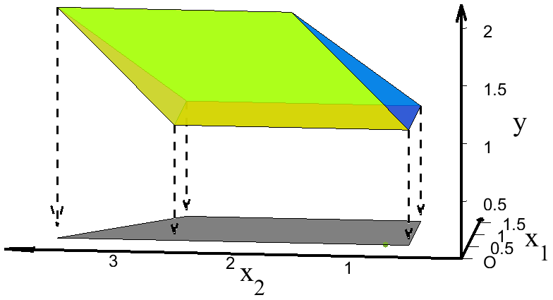
Figure 2 shows that the ADJ oracle takes the facet $\left\{{\mathit{a}}_f^{\mathrm{T}}\mathit{x}=b_f\right\}\cap \mathit{\pi }\left(P\right)$ of P (the blue line segment in this example) and ridge $\left\{{\mathit{a}}_r^{\mathrm{T}}\mathit{x}=b_r\right\}\cap {\mathit{\pi }}_d\left(P_{E_f}\right)$ (the intersection of the blue line segment and the yellow line segment in this example) to solve the adjacent facet (the yellow line segment in this example is the facet to be solved), and x^* is the intersection of plane ${\mathit{a}}_f^{\mathrm{T}}\mathit{x}=b_f\left(\mathrm{1}-\mathit{\epsilon }\right)$ and the yellow line segment.

Figure 2 The ADJ oracle in Example 1.

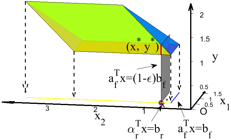
All the points on the red line segment of P can be projected onto x^*, which indicates that all points on the red line segment are optimal solutions of the LP problem. The optimal solution domain belongs to the yellow facet of $P_{E_{\mathrm{adj}}}$, and its corresponding equality set is E_adj={4}.

However, most of the LP solvers will only give one optimal solution for the LP problem with multiple optimal solutions. If this solution is mistakenly considered the only optimal solution, this may lead to the iteration cycle and increase the computational burden.

In this case, if $\left(x^{*},y^{*}\right)$ on the intersection of the blue facet and yellow facet is taken as the unique optimal solution, the $P_{{E^{\prime }}_{\mathrm{adj}}}$ that $\left(x^{*},y^{*}\right)$ belongs to is the intersection line of the blue and yellow facets of P, $E_{\mathrm{adj}}^{\prime }=\left\{\mathrm{1},\mathrm{4}\right\}$. According to Fig. 3, $P_{{E^{\prime }}_{\mathrm{adj}}}\subset P_{E_{\mathrm{adj}}}$ and ${\mathit{\pi }}_d\left(P_{{E^{\prime }}_{\mathrm{adj}}}\right)\subset {\mathit{\pi }}_d\left(P_{E_{\mathrm{adj}}}\right)$.

Figure 3 The non-uniqueness of the optimal solution is ignored.

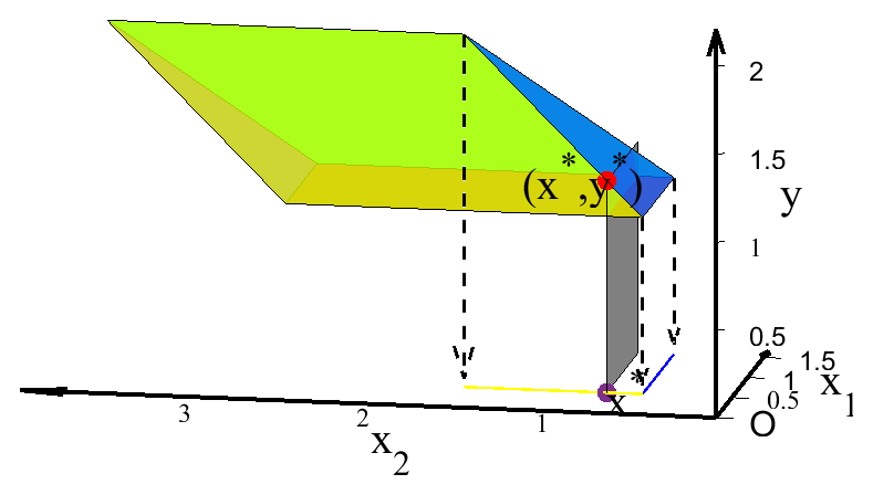
Owing to $\text{aff}{\mathit{\pi }}_d\left(P_{{E^{\prime }}_{\mathrm{adj}}}\right)=\text{aff}{\mathit{\pi }}_d\left(P_{E_{\mathrm{adj}}}\right)$, some facets may appear multiple times in the following iterative process, which may increase the number of iterations, and even the algorithm cannot be terminated.

3.2 Shortcomings of the original algorithm

The barriers of the original ESP algorithm in the case of dual degeneracy can be listed as follows.

• i.

  Currently, most of the LP solvers do not have the ability to judge the uniqueness of the solutions of linear programming. Although several achievements have been made on the unique conditions of LP solutions (Mangasarian, 1979), these methods are difficult to embed into the existing LP solvers, since they induce additional computation.

• ii.

  Since the dual degeneracy is only a necessary but insufficient condition for linear programming to have multiple optimizers (Borrelli et al., 2017), it is conservative to determine the uniqueness of the solution by testing whether the dual degeneracy occurs in Jones et al. (2004).

• iii.

  Expression (3) implies that, in the case of d≥3, the value of x^* is always not unique; i.e., the LP problem always has multiple optimal solutions. However, if only the value of x^* is not unique and the value of y^* is unique, irrespective of the point in the optimal solution space, it can be regarded as the unique optimal solution, and the obtained $P_{E_{\mathrm{adj}}}$ does not vary. In this case, an extra computation is added to handle the non-uniqueness of the optimal solution of the LP.

3.3 Alternative criteria

According to Example (1), there may be multiple faces $P_{E_f}$ in P, and the projections of their affine hulls are all aff F_π. The collection of all E_f satisfying this condition can be denoted as

$$\begin{array}{}\text{(4)}& \begin{array}{rl}{\mathrm{\Xi }}_{F_{\mathit{\pi }}}& =\mathit{\{}{E}_f\subset \left\{\mathrm{1},\mathrm{2},\mathrm{\dots },q\right\}\left|{\mathit{\pi }}_d\left(\text{aff}{P}_{E_f}\right)\right.\\ & =\text{aff}{F}_{\mathit{\pi }},G\left(E_f\right)=E_f\mathit{\}},\end{array}\end{array}$$

where

$$\begin{array}{rl}& G\left(E_f\right)=\mathit{\{}i\in \left\{\mathrm{1},\mathrm{2},\mathrm{\dots },q\right\}|{\mathbf{C}}_i\mathit{x}+{\mathbf{D}}_i\mathit{y}=b_i,\\ & \forall (\mathit{x},\mathit{y})\in P_{E_f}\mathit{\}}.\end{array}$$

The discussion on the uniqueness of optimizers of LP is to ensure that the obtained E_f is the element in ${\mathrm{\Xi }}_{F_{\mathit{\pi }}}$ with the maximal $\text{dim}{P}_{E_f}$. The primary result can be stated as given below.
Theorem 3.1 Consider the ${\mathrm{\Xi }}_{F_{\mathit{\pi }}}$ defined in Expression (4), and E_f is the subset of ${\mathrm{\Xi }}_{F_{\mathit{\pi }}}$ that maximizes the value of $\text{dim}{P}_{E_f}$ if and only if there are no zero rows in $\mathbf{N}\left({\mathbf{D}}_{E_f}^{\mathrm{T}}\right)$.
Proof (sufficient part): the sufficiency of Theorem 3.1 has been proven by the following inverse negative proposition.

If there exist zero rows in $\mathbf{N}\left({\mathbf{D}}_{E_f}^{\mathrm{T}}\right)$, then E_f is not the element in ${\mathrm{\Xi }}_{F_{\mathit{\pi }}}$ that maximizes the value of $\text{dim}{P}_{E_f}$.

Let $E_f=\left\{e_{\mathrm{1}},e_{\mathrm{2}},\mathrm{\dots },e_n,\right\}$, ${\mathbf{D}}_E^{\mathrm{T}}=\left[\begin{array}{cccc}{\mathbf{D}}_{e_{\mathrm{1}}}^{\mathrm{T}}& {\mathbf{D}}_{e_{\mathrm{2}}}^{\mathrm{T}}& \mathrm{\dots }& {\mathbf{D}}_{e_n}^{\mathrm{T}}\end{array}\right]$; without loss of generality, we can assume that the last m rows of $\mathbf{N}\left({\mathbf{D}}_{E_f}^{\mathrm{T}}\right)$ are zero rows.

$$\begin{array}{rl}& \mathbf{N}\left({\mathbf{D}}_{E_f}^{\mathrm{T}}\right)=\left[\begin{array}{cccc}{N}_{\mathrm{1}}& N_{\mathrm{2}}& \mathrm{\dots }& N_{n-r}\end{array}\right]\\ & =\left[\begin{array}{cccc}{N}_{\mathrm{11}}& N_{\mathrm{12}}& \mathrm{\cdots }& N_{\mathrm{1}\left(n-r\right)}\\ N_{\mathrm{21}}& N_{\mathrm{22}}& \mathrm{\cdots }& N_{\mathrm{2}\left(n-r\right)}\\ \mathrm{⋮}& \mathrm{⋮}& \mathrm{\ddots }& \mathrm{⋮}\\ N_{\left(n-m\right)\mathrm{1}}& N_{\left(n-m\right)\mathrm{2}}& \mathrm{\cdots }& N_{\left(n-m\right)\left(n-r\right)}\\ \mathrm{0}& \mathrm{0}& \mathrm{\cdots }& \mathrm{0}\\ \mathrm{⋮}& \mathrm{⋮}& \mathrm{\ddots }& \mathrm{⋮}\\ \mathrm{0}& \mathrm{0}& \mathrm{\cdots }& \mathrm{0}\end{array}\right]\\ & =\left[\begin{array}{c}{N}_{\mathrm{1}}^{\mathrm{row}}\\ N_{\mathrm{2}}^{\mathrm{row}}\\ \mathrm{⋮}\\ N_{n-m}^{\mathrm{row}}\\ N_{n-m+\mathrm{1}}^{\mathrm{row}}\\ \mathrm{⋮}\\ N_n^{\mathrm{row}}\end{array}\right]\end{array}.$$

According to ${\mathbf{D}}_{E_f}^{\mathrm{T}}\mathbf{N}\left({\mathbf{D}}_{E_f}^{\mathrm{T}}\right)=\sum _{i=\mathrm{1}}^n{\mathbf{D}}_{e_i}^{\mathrm{T}}{N}_i^{\mathrm{row}}=\mathrm{0}$, there is a one-to-one correspondence between $N_i^{\mathrm{row}}$ and ${\mathbf{D}}_{ei}^{\mathrm{T}}$; i.e., there is a one-to-one correspondence between the rows of $\mathbf{N}\left({\mathbf{D}}_{E_f}^{\mathrm{T}}\right)$ and the elements of E_f.

Let $E_f^{\prime }=\left\{e_{\mathrm{1}},e_{\mathrm{2}},\mathrm{\dots },e_{n-m}\right\}$.

$$\begin{array}{rl}& \mathbf{N}\left({\mathbf{D}}_{E_f}^{\mathrm{T}}\right)=\left[\begin{array}{cccc}{N}_{\mathrm{1}}& N_{\mathrm{2}}& \mathrm{\cdots }& N_{n-r}\end{array}\right]\\ & =\left[\begin{array}{cccc}{N}_{\mathrm{11}}& N_{\mathrm{12}}& \mathrm{\cdots }& N_{\mathrm{1}\left(n-r\right)}\\ N_{\mathrm{21}}& N_{\mathrm{22}}& \mathrm{\cdots }& N_{\mathrm{2}\left(n-r\right)}\\ \mathrm{⋮}& \mathrm{⋮}& \mathrm{\ddots }& \mathrm{⋮}\\ N_{\left(n-m\right)\mathrm{1}}& N_{\left(n-m\right)\mathrm{2}}& \mathrm{\cdots }& N_{\left(n-m\right)\left(n-r\right)}\\ \mathrm{0}& \mathrm{0}& \mathrm{\cdots }& \mathrm{0}\\ \mathrm{⋮}& \mathrm{⋮}& \mathrm{\ddots }& \mathrm{⋮}\\ \mathrm{0}& \mathrm{0}& \mathrm{\cdots }& \mathrm{0}\end{array}\right]\\ & =\left[\begin{array}{c}{N}_{\mathrm{1}}^{\mathrm{row}}\\ N_{\mathrm{2}}^{\mathrm{row}}\\ \mathrm{⋮}\\ N_{n-m}^{\mathrm{row}}\\ N_{n-m+\mathrm{1}}^{\mathrm{row}}\\ \mathrm{⋮}\\ N_n^{\mathrm{row}}\end{array}\right]\end{array}$$

$\left[\begin{array}{cccc}{N}_{\mathrm{1}}& N_{\mathrm{2}}& \mathrm{\dots }& N_{n-r}\end{array}\right]$ forms a basis for the null space of ${\mathbf{D}}_{E_f}^{\mathrm{T}}$, implying that $\left[\begin{array}{cccc}{N}_{\mathrm{1}}^{\prime }& N_{\mathrm{2}}^{\prime }& \mathrm{\dots }& N_{n-r}^{\prime }\end{array}\right]$ forms a basis for the null space of ${\mathbf{D}}_{E_f^{\prime }}^{\mathrm{T}}$.

Next, we will prove that $E_f^{\prime }$ is an equality set, i.e.,

$$E_f^{\prime }=\left\{i\in \left\{\mathrm{1},\mathrm{\cdots },q\right\}|{\mathbf{C}}_i\mathit{x}+{\mathbf{D}}_i\mathit{y}=b_i,\forall \left(\mathit{x},\mathit{y}\right)\in P_{E_f^{\prime }}\right\}.$$

Since E_f is an equation set, we only need to prove that

$$\forall e_i\in E_f^{\prime \prime },\exists (\mathit{x},\mathit{y})\in P_{E_f^{\prime }},\text{s.t.}{\mathbf{C}}_i\mathit{x}+{\mathbf{D}}_i\mathit{y}\ne b_i,$$

where

$$E_f^{\prime \prime }=\left\{e_{n-m+\mathrm{1}},e_{n-m+\mathrm{2}},\mathrm{\cdots },e_n\right\}.$$

Since ${\mathbf{D}}_{E_f\backslash \left\{e_i\right\}}^{\mathrm{T}}\mathbf{N}\left({\mathbf{D}}_{E_f\backslash \left\{\left\{e_i\right\}\right\}}^{\mathrm{T}}\right)=\mathrm{0}$, the null space of ${\mathbf{D}}_{E_f}^{\mathrm{T}}$ and ${\mathbf{D}}_{E_f\backslash \left\{e_i\right\}}^{\mathrm{T}}$ has the same number of bases, and thus

$$\begin{array}{}\text{(5)}& \text{rank}{\mathbf{D}}_{E_f}^{\mathrm{T}}-\text{rank}{\mathbf{D}}_{E_f\backslash \left\{e_i\right\}}^{\mathrm{T}}=\mathrm{1}.\end{array}$$

Equation (5) implies that

$$\begin{array}{}\text{(6)}& \text{rank}\left[{\mathbf{C}}_{E_f}{\mathbf{D}}_{E_f}\right]-\text{rank}\left[{\mathbf{C}}_{E_f\backslash \left\{e_i\right\}}{\mathbf{D}}_{E_f\backslash \left\{e_i\right\}}\right]=\mathrm{1}.\end{array}$$

Then, combining Proposition 2.5 with Expression (6), we get

$$\begin{array}{}\text{(7)}& \text{dim}{P}_{E_f}=k+d-\text{rank}\left[{\mathbf{C}}_{E_f}{\mathbf{D}}_{E_f}\right]=\text{dim}{P}_{E_f\backslash \left\{e_i\right\}}-\mathrm{1}.\end{array}$$

$E_{E_f\backslash \left\{e_i\right\}}\subset E_f$ implies that

$$\begin{array}{}\text{(8)}& P_{E_f\backslash \left\{e_i\right\}}\supseteq P_{E_f}.\end{array}$$

Combining Expressions (7) and (8) gives us

$$P_{E_f\backslash \left\{e_i\right\}}\supset P_{E_f}.$$

Thus, $P_{E_f\backslash \left\{e_i\right\}}\backslash P_{E_f}\ne \mathit{\varphi }$. Let $\mathit{x}\in P_{E_f\backslash \left\{e_i\right\}}\backslash P_{E_f}$, ${\mathbf{C}}_i\mathit{x}+{\mathbf{D}}_i\mathit{y}\ne b_i$, and thus $E_f^{\prime }$ is an equality set. We can verify that

$$\begin{array}{c}{\displaystyle }\mathbf{N}{\left({\mathbf{D}}_{E_f}^{\mathrm{T}}\right)}^{\mathrm{T}}{\mathbf{C}}_{E_f}=\mathbf{N}{\left({\mathbf{D}}_{{E^{\prime }}_f}^{\mathrm{T}}\right)}^{\mathrm{T}}{\mathbf{C}}_{{E^{\prime }}_f},\\ {\displaystyle }\mathbf{N}{\left({\mathbf{D}}_{E_f}^{\mathrm{T}}\right)}^{\mathrm{T}}{b}_{E_f}=\mathbf{N}{\left({\mathbf{D}}_{{E^{\prime }}_f}^{\mathrm{T}}\right)}^{\mathrm{T}}{b}_{{E^{\prime }}_f}.\end{array}$$

From Proposition 2.4, $\text{aff}{P}_{E_f^{\prime }}=\text{aff}{P}_{E_f}$, and thus $E_f^{\prime }\in {\mathrm{\Xi }}_{F_{\mathit{\pi }}}$. Therefore, $\text{dim}{P}_{E_f^{\prime }}\ge \text{dim}{P}_{E_f\backslash \left\{e_i\right\}}>\text{dim}{P}_{E_f}$, and the sufficient part is proven.

Necessary part: the necessary part is proven by contradiction.

Suppose that each row in $\mathbf{N}\left({\mathbf{D}}_{E_f}^{\mathrm{T}}\right)$ is not a zero row. If $\exists {E_f}^{*}\in {\mathrm{\Xi }}_{F_{\mathit{\pi }}}$, then $\text{dim}{P}_{{E_f}^{*}}>\text{dim}{P}_{E_f}$. Let $\text{dim}{P}_{{E_f}^{*}}-\text{dim}{P}_{E_f}=n_c$, since the projections of ${E_f}^{*}$ and E_f have the same affine hull. This can be obtained from Proposition 2.5:

$$\text{rank}{\mathbf{D}}_{E_f}-\text{rank}{\mathbf{D}}_{{E_f}^{*}}=n_c,$$

since ${\mathit{\pi }}_d\left(\text{aff}{P}_{E_f}\right)={\mathit{\pi }}_d\left(\text{aff}{P}_{E_f}^{*}\right)$. Proposition 2.4 implies that $\mathbf{N}\left({\mathbf{D}}_{E_f}^{\mathrm{T}}\right)$ and $\mathbf{N}\left({\mathbf{D}}_{{E_f}^{*}}^{\mathrm{T}}\right)$ have the same number of columns, i.e., $n^{*}-\text{rank}{\mathbf{D}}_{{E_f}^{*}}=n-\text{rank}{\mathbf{D}}_{E_f}$, $n-n^{*}=n_c$.

We can denote $\mathbf{N}\left({\mathbf{D}}_{E_f^{*}}^{\mathrm{T}}\right)$ as follows.

$$\begin{array}{rl}& \mathbf{N}\left({\mathbf{D}}_{E_f^{*}}^{\mathrm{T}}\right)=\left[\begin{array}{cccc}{N}_{\mathrm{1}}^{*}& N_{\mathrm{2}}^{*}& \mathrm{\dots }& N_{n-r}^{*}\end{array}\right]\\ & =\left[\begin{array}{cccc}{N}_{\mathrm{11}}^{*}& N_{\mathrm{12}}^{*}& \mathrm{\cdots }& N_{\mathrm{1}(n-r)}^{*}\\ N_{\mathrm{21}}^{*}& N_{\mathrm{22}}& \mathrm{\cdots }& N_{\mathrm{2}(n-r)}^{*}\\ \mathrm{⋮}& \mathrm{⋮}& \mathrm{\ddots }& \mathrm{⋮}\\ N_{\left(n^{*}\right)\mathrm{1}}& N_{\left(n^{*}\right)\mathrm{2}}& \mathrm{\cdots }& N_{\left(n^{*}\right)(n-r)}\end{array}\right]\end{array}$$

Then, we add n_c zero elements to each column of $\mathbf{N}\left({\mathbf{D}}_{E_f^{*}}^{\mathrm{T}}\right)$ as follows.

$$\begin{array}{rl}& \mathbf{N}\left({\mathbf{D}}_{E_f^{*}}^{\prime \mathrm{T}}\right)=\left[\begin{array}{cccc}{N}_{\mathrm{1}}^{\prime *}& N_{\mathrm{2}}^{\prime *}& \mathrm{\dots }& N_{n-r}^{\prime *}\end{array}\right]\\ & =\left[\begin{array}{cccc}{N}_{\mathrm{11}}^{*}& N_{\mathrm{12}}^{*}& \mathrm{\cdots }& N_{\mathrm{1}(n-r)}^{*}\\ N_{\mathrm{21}}^{*}& N_{\mathrm{22}}& \mathrm{\cdots }& N_{\mathrm{2}(n-r)}^{*}\\ \mathrm{⋮}& \mathrm{⋮}& \mathrm{\ddots }& \mathrm{⋮}\\ N_{\left(n^{*}\right)\mathrm{1}}& N_{\left(n^{*}\right)\mathrm{2}}& \mathrm{\cdots }& N_{\left(n^{*}\right)(n-r)}\\ \mathrm{0}& \mathrm{0}& \mathrm{\cdots }& \mathrm{0}\\ \mathrm{⋮}& \mathrm{⋮}& \mathrm{\ddots }& \mathrm{⋮}\\ \mathrm{0}& \mathrm{0}& \mathrm{\cdots }& \mathrm{0}\end{array}\right]\end{array}$$

Since $N_{\mathrm{1}}^{\prime *}$, $N_{\mathrm{2}}^{\prime *},\mathrm{\dots },N_{n-r}^{\prime *}$ are linearly independent, $N_{\mathrm{1}}^{\prime *}$, $N_{\mathrm{2}}^{\prime *},\mathrm{\dots },N_{n-r}^{\prime *}$ are bases of ${\mathbf{D}}_{E_f}^{\mathrm{T}}$. There are no zero rows in $\mathbf{N}\left({\mathbf{D}}_{E_f}^{\mathrm{T}}\right)$, and thus N₁, $N_{\mathrm{2}},\mathrm{\dots },N_{n-r}$ cannot be expressed linearly by $N_{\mathrm{1}}^{\prime *}$, $N_{\mathrm{2}}^{\prime *},\mathrm{\dots },N_{n-r}^{\prime *}$, which is a contradiction. Therefore, the necessary part is proven.

Corollary 3.1 Let $E_f=\left\{e_{\mathrm{1}},e_{\mathrm{2}},\mathrm{\dots },e_n,\right\}\in {\mathrm{\Xi }}_{F_{\mathit{\pi }}}$. If there exist zero rows in $\mathbf{N}\left({\mathbf{D}}_{E_f}^{\mathrm{T}}\right)$, then $E_f^{\prime }$, which consists of elements of E_f corresponding to non-zero rows in $\mathbf{N}\left({\mathbf{D}}_{E_f}^{\mathrm{T}}\right)$, is the element in ${\mathrm{\Xi }}_{F_{\mathit{\pi }}}$ that maximizes the value of $\text{dim}{P}_{E_f}$.

Corollary 3.1 is a direct consequence of Theorem 3.1, and it implies that it is no longer necessary to discuss the uniqueness of the solutions in the SHOOT and ADJ oracles. However, it only takes an arbitrary solution as the unique solution and then gets the E_f that maximizes the value of $\text{dim}{P}_{E_f}$ in ${\mathrm{\Xi }}_{F_{\mathit{\pi }}}$.

3.3.1 Improved SHOOT oracle

Step 1 (selecting a direction γ and finding a point on the surface of P)

By randomly choosing γ∈R^d, we solve the following linear programming.

$$\begin{array}{}\text{(9)}& \begin{array}{l}\left(r^{*},{\mathit{y}}^{*}\right)=\underset{(r,\mathit{y})\in R\times R^k}{\arg max}r\\ \text{s.t.}\mathbf{C}\mathit{\gamma }r+\mathbf{D}\mathit{y}\le \mathit{b}\end{array}\end{array}$$

Step 2 (whether a facet of π_d(P) is found)

$$\begin{array}{}\text{(10)}& E_{f_{\mathrm{0}}}=\left\{i|{\mathbf{C}}_i\mathit{\gamma }r+{\mathbf{D}}_i\mathit{y}=b_i\right\}\end{array}$$

If $\text{Rank}\left(\mathbf{N}{\left({\mathbf{D}}_{E_{f_{\mathrm{0}}}}^{\mathrm{T}}\right)}^{\mathrm{T}}{\mathbf{C}}_{E_{f_{\mathrm{0}}}}\right)=\mathrm{1}$, continue. Otherwise, go to Step 1.

Step 3 (ensuring the $E_{f_{\mathrm{0}}}$ is the element with the maximal $\text{dim}{P}_{{E_f}_{\mathrm{0}}}$ in ${\mathrm{\Xi }}_{F_{\mathit{\pi }}}$)

If there exist zero rows in $\mathbf{N}\left({\mathbf{D}}_{E_{f_{\mathrm{0}}}}^{\mathrm{T}}\right)$, let $E_{f_{\mathrm{0}}}\leftarrow E_{f_{\mathrm{0}}}^{\prime }$ as Corollary 3.1. Otherwise, continue.

Step 4 (computing the affine hull of the facet and normalizing)

$$\begin{array}{l}\left[{\mathit{a}}_f^{\mathrm{T}},b_f\right]=\mathbf{N}{\left({\mathbf{D}}_{E_{f_{\mathrm{0}}}}^{\mathrm{T}}\right)}^{\mathrm{T}}\left[{\mathbf{C}}_{E_{f_{\mathrm{0}}}},b_{E_{f_{\mathrm{0}}}}\right]\\ \left[{\mathit{a}}_f^{\mathrm{T}},b_f\right]={\displaystyle \frac{\text{sign}{b}_f}{{∥{\mathit{a}}_f∥}_{\mathrm{2}}}}\left[{\mathit{a}}_f^{\mathrm{T}},b_f\right]\end{array}$$

3.3.2 Improved ADJ oracle

Step 1 (finding a point on the adjacent facet of π_d(P) and its corresponding pre-image)

Solve the following linear programming.

$$\begin{array}{l}\left({\mathit{x}}^{*},{\mathit{y}}^{*}\right)=\underset{\mathit{x},\mathit{y}}{\arg max}{\mathit{a}}_r^{\mathrm{T}}\mathit{x}\\ \begin{array}{rl}\text{s.t.}& {\mathbf{C}}_{E_r}\mathit{x}+{\mathbf{D}}_{E_r}\mathit{y}\le b_{E_r},\\ & {\mathit{a}}_f^{\mathrm{T}}\mathit{x}=b_f\left(\mathrm{1}-\mathit{\epsilon }\right)\end{array}\end{array}$$

Step 2 (searching for the E_f of ${\mathrm{\Xi }}_{F_{\mathit{\pi }}}$ that maximizes the value of $\text{dim}{P}_{E_f}$)

$$E_{\mathrm{adj}}\leftarrow \left\{i\in E_r\left|{\mathbf{C}}_i{x}^{*}+{\mathbf{D}}_i{y}^{*}=b_i\right.\right\}$$

If there exist zero rows in $\mathbf{N}\left({\mathbf{D}}_{E_{\mathrm{adj}}}^{\mathrm{T}}\right)$, let $E_{\mathrm{adj}}\leftarrow E_{\mathrm{adj}}^{\prime }$ as Corollary 3.1. Otherwise, continue.

Step 3 (computing the affine hull of the adjacent facet and normalizing)

$$\begin{array}{l}\left[{\mathit{a}}_{\mathrm{adj}}^{\mathrm{T}},b_{\mathrm{adj}}\right]=\mathbf{N}{\left({\mathbf{D}}_{E_{\mathrm{adj}}}^{\mathrm{T}}\right)}^{\mathrm{T}}\left[{\mathbf{C}}_{E_{\mathrm{adj}}},b_{E_{\mathrm{adj}}}\right]\\ \left[{\mathit{a}}_{\mathrm{adj}}^{\mathrm{T}},b_{\mathrm{adj}}\right]={\displaystyle \frac{\text{sign}{b}_{\mathrm{adj}}}{{∥{\mathit{a}}_{\mathrm{adj}}∥}_{\mathrm{2}}}}\left[{\mathit{a}}_{\mathrm{adj}}^{\mathrm{T}},b_{\mathrm{adj}}\right]\end{array}$$

4 An improved strategy without searching for E_r

In this section, we first explain the obstacles to searching for E_r in the case of $\text{dim}{P}_{E_f}>d-\mathrm{1}$, an improved strategy that does not require E_r is proposed, and then a new criterion is given to judge whether the two ridges are the same.

4.1 The barrier to searching for E_r

In the RDG oracle, if $\text{dim}{P}_{E_f}>d-\mathrm{1}$, this requires a recursive call to the ESP algorithm that reduces the dimension onto which we are projecting at each step.

We note that a_r and b_r can easily be obtained through this strategy, but it is often expensive to search for E_r. The only way to do this is to list all of the equality sets $E_c=\left\{\mathrm{1},\mathrm{2},\mathrm{\dots },q\right\}\backslash E_f$, $\left\{E_p^i=E_f\cup E_i\right\}$, and E_i⊂E_c, and searching for the ${\mathit{\pi }}_d\left(E_p^i\right)$ is equal to $\left\{\mathit{x}\left|{\stackrel{\mathrm{̃}}{\mathit{a}}}_f^{\mathrm{T}}\stackrel{\mathrm{̃}}{\mathit{x}}={\stackrel{\mathrm{̃}}{b}}_f\right.\right\}\cap {\mathit{\pi }}_{d-\mathrm{1}}\left(\stackrel{\mathrm{̃}}{P}\right)$. The computational effort increases in an exponential manner in the number of dimensions.

4.2 New criteria without E_r

To improve the computational efficiency of the algorithm when the optimizer of LP is not unique, the search for E_r has been abandoned. However, in the original ESP algorithm, E_r is needed to judge the occurrence times of ridges, and hence we have proposed a new criterion to judge whether the two ridges in π_d(P) are the same without E_r.

Lemma 4.1 Let P be a polytope. $F_{\mathrm{1}}=\left\{\mathit{x}|{\mathit{a}}_{f_{\mathrm{1}}}^{\mathrm{T}}\mathit{x}=b_{f_{\mathrm{1}}}\right\}\cap {\mathit{\pi }}_d\left(P\right)$ and $F_{\mathrm{2}}=\left\{\mathit{x}|{\mathit{a}}_{f_{\mathrm{2}}}^{\mathrm{T}}\mathit{x}=b_{f_{\mathrm{2}}}\right\}\cap {\mathit{\pi }}_d\left(P\right)$ are the facets of P, $R_{\mathrm{1}}=\left\{\mathit{x}|{\mathit{a}}_{r_{\mathrm{1}}}^{\mathrm{T}}\mathit{x}=b_{r_{\mathrm{2}}}\right\}\cap F_{\mathrm{1}}$ and $R_{\mathrm{2}}=\left\{\mathit{x}|{\mathit{a}}_{r_{\mathrm{2}}}^{\mathrm{T}}\mathit{x}=b_{r_{\mathrm{2}}}\right\}\cap F_{\mathrm{2}}$ are the ridges of P, and R₁⊂F₁ and R₂⊂F₂. Then, $F_{\mathrm{1}}\cap F_{\mathrm{2}}=R_{\mathrm{1}}=R_{\mathrm{2}}$ if and only if

$$\begin{array}{}\text{(11)}& \text{rank}\left[\begin{array}{c}{\mathit{a}}_{f_{\mathrm{1}}}^{\mathrm{T}}\\ {\mathit{a}}_{f_{\mathrm{2}}}^{\mathrm{T}}\\ {\mathit{a}}_{r_{\mathrm{1}}}^{\mathrm{T}}\\ {\mathit{a}}_{r_{\mathrm{2}}}^{\mathrm{T}}\end{array}\right]=\text{rank}\left[\begin{array}{cc}{\mathit{a}}_{f_{\mathrm{1}}}^{\mathrm{T}}& b_{f_{\mathrm{1}}}\\ {\mathit{a}}_{f_{\mathrm{2}}}^{\mathrm{T}}& b_{f_{\mathrm{2}}}\\ {\mathit{a}}_{r_{\mathrm{1}}}^{\mathrm{T}}& b_{r_{\mathrm{1}}}\\ {\mathit{a}}_{r_{\mathrm{2}}}^{\mathrm{T}}& b_{r_{\mathrm{2}}}\end{array}\right]=\mathrm{2}.\end{array}$$

Proof Only the proof of sufficiency is given here, and the necessity is obvious. Since ${\mathit{a}}_{f_{\mathrm{1}}}\perp {\mathit{a}}_{r_{\mathrm{1}}},{\mathit{a}}_{f_{\mathrm{2}}}\perp {\mathit{a}}_{r_{\mathrm{2}}}$,

$$\begin{array}{}\text{(12)}& \text{rank}\left[\begin{array}{cc}{\mathit{a}}_{f_{\mathrm{1}}}^{\mathrm{T}}& b_{f_{\mathrm{1}}}\\ {\mathit{a}}_{r_{\mathrm{1}}}^{\mathrm{T}}& b_{r_{\mathrm{1}}}\end{array}\right]=\text{rank}\left[\begin{array}{cc}{\mathit{a}}_{f_{\mathrm{2}}}^{\mathrm{T}}& b_{f_{\mathrm{2}}}\\ {\mathit{a}}_{r_{\mathrm{2}}}^{\mathrm{T}}& b_{r_{\mathrm{2}}}\end{array}\right]=\mathrm{2}.\end{array}$$

Combining Expression (11) with Expression (12) gives us

$$\begin{array}{rl}& \left\{\mathit{x}|{\mathit{a}}_{r_{\mathrm{1}}}^{\mathrm{T}}\mathit{x}=b_{r_{\mathrm{1}}}\right\}\cap \left\{\mathit{x}|{\mathit{a}}_{f_{\mathrm{2}}}^{\mathrm{T}}\mathit{x}=b_{f_{\mathrm{2}}}\right\}\\ & =\left\{\mathit{x}|{\mathit{a}}_{r_{\mathrm{2}}}^{\mathrm{T}}\mathit{x}=b_{r_{\mathrm{2}}}\right\}\cap \left\{\mathit{x}|{\mathit{a}}_{f_{\mathrm{2}}}^{\mathrm{T}}\mathit{x}=b_{f_{\mathrm{2}}}\right\}.\end{array}$$

Note that

$$\begin{array}{l}{R}_{\mathrm{2}}=\left\{\mathit{x}|{\mathit{a}}_{r_{\mathrm{2}}}^{\mathrm{T}}\mathit{x}=b_{r_{\mathrm{2}}}\right\}\cap \left\{\mathit{x}|{\mathit{a}}_{f_{\mathrm{2}}}^{\mathrm{T}}\mathit{x}=b_{f_{\mathrm{2}}}\right\}\cap {\mathit{\pi }}_d\left(P\right),\\ R_{\mathrm{1}}=\left\{\mathit{x}|{\mathit{a}}_{r_{\mathrm{1}}}^{\mathrm{T}}\mathit{x}=b_{r_{\mathrm{1}}}\right\}\cap \left\{\mathit{x}|{\mathit{a}}_{f_{\mathrm{1}}}^{\mathrm{T}}\mathit{x}=b_{f_{\mathrm{1}}}\right\}\cap {\mathit{\pi }}_d\left(P\right),\end{array}$$

and thus R₁=R₂. Since the two facets of the polytope can only have one common ridge, $F_{\mathrm{1}}\cap F_{\mathrm{2}}=R_{\mathrm{1}}=R_{\mathrm{2}}$.

4.3 Some other patches caused by the abandonment of searching for E_r

Since E_r is required in other steps in the original ESP algorithm, certain other patches need to be made.

In the ADJ oracle, LP (9) and Eq. (10) can be changed to LP (13) and Eq. (14), respectively.

$$\begin{array}{}\text{(13)}& \begin{array}{l}\left({\mathit{x}}^{*},{\mathit{y}}^{*}\right)=\underset{\mathit{x},\mathit{y}}{\arg max}{\mathit{a}}_r^{\mathrm{T}}\mathit{x}\\ \begin{array}{rl}\text{s.t.}& \mathbf{C}\mathit{x}+\mathbf{D}\mathit{y}\le \mathit{b},\\ & {\mathit{a}}_f^{\mathrm{T}}\mathit{x}=b_f\left(\mathrm{1}-\mathit{\epsilon }\right)\end{array}\end{array}\end{array}$$

$$\begin{array}{}\text{(14)}& E_{\mathrm{adj}}\leftarrow \left\{i\in \left\{\mathrm{1},\mathrm{2},\mathrm{\dots },q\right\}\left|{\mathbf{C}}_i{\mathit{x}}^{*}+{\mathbf{D}}_i{\mathit{y}}^{*}=b_i\right.\right\}\end{array}$$

We can verify that the modified algorithm still gets the correct result, though it also adds certain extra computation cost in the case of $\text{dim}{P}_{E_f}=d-\mathrm{1}$. We note that $\text{dim}\left(P_{E_f}\right)>d-\mathrm{1}$ if and only if the optimizer of LP is non-unique. A switching strategy can be adopted to take the original method until the optimizer of LP is non-unique.

5 Numerical simulations

In this section, the effectiveness of the proposed method is verified based on certain typical orthogonal projection cases and applications to N-step controllable set calculations in the control field.

5.1 Numerical simulations for the typical orthogonal projection cases

We select three cases for numerical simulation, and two of them are dual-degenerate, though one is not dual-degenerate.

• i.

  The projection of a three-dimensional n prism with n+2 half-spaces onto a two-dimensional plane

• ii.

  The projection of an n-dimensional cube with 2n half-spaces onto a two-dimensional plane

• iii.

  The projection of an n-dimensional cube onto a three-dimensional space

In cases (i) and (ii), the dual degeneracy occurs, whereas there is no dual degeneracy in case (iii). The simulation operation has been implemented in MATLAB 2019, and the running times of the original ESP and the improved ESP are shown in Fig. 4.

Figure 4 Comparative running times for typical cases.

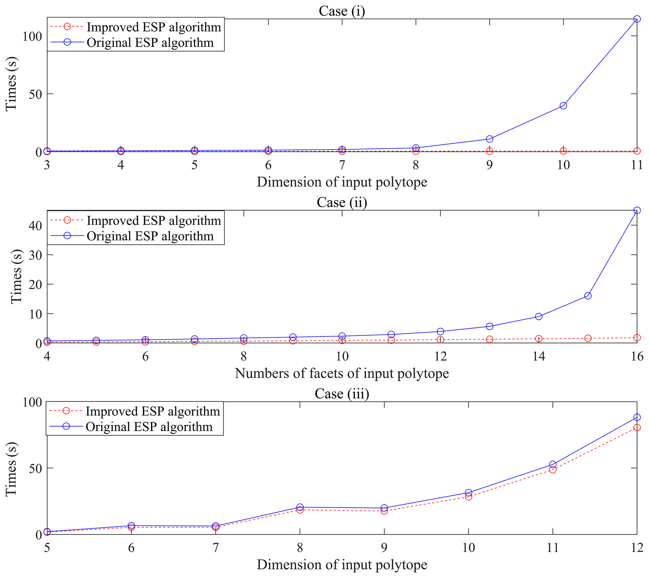
The running time of the original ESP algorithm increases exponentially with dimensions and the number of half-planes of the input polytopes under the dual-degeneracy cases, whereas the improved ESP algorithm significantly reduces the computational burden in the case of dual degeneracy. The running time is also optimized in the case of non-dual degeneracy, since it is no longer necessary to judge the uniqueness of linear programming solutions in the improved ESP algorithm.

5.2 Applications to N-step controllable set calculations

We apply the proposed method for the calculation of N-step controllable sets in the control field, and the problem setup is described as given below.

Consider the following linear discrete system.

$$\left[\begin{array}{c}{x}_{\mathrm{1}}(k+\mathrm{1})\\ x_{\mathrm{2}}(k+\mathrm{1})\end{array}\right]=\underset{\mathbf{A}}{\underbrace{\left[\begin{array}{cc}\mathrm{1.1}& \mathrm{2}\\ \mathrm{0}& \mathrm{0.95}\end{array}\right]}}\left[\begin{array}{c}{x}_{\mathrm{1}}\left(k\right)\\ x_{\mathrm{2}}\left(k\right)\end{array}\right]+\underset{\mathbf{B}}{\underbrace{\left[\begin{array}{c}\mathrm{0}\\ \mathrm{0.0787}\end{array}\right]}}\mathit{u}$$

$\mathit{x}={\left[x_{\mathrm{1}},x_{\mathrm{2}}\right]}^{\mathrm{T}}$ and u are the state and input vectors, respectively, subject to the constants as follows.

$$\underset{{\mathbf{A}}_x}{\underbrace{\left[\begin{array}{cc}\mathrm{0.125}& \mathrm{0}\\ -\mathrm{0.125}& \mathrm{0}\\ \mathrm{0}& \mathrm{0.125}\\ \mathrm{0}& -\mathrm{0.125}\end{array}\right]}}\left[\begin{array}{c}{x}_{\mathrm{1}}\\ x_{\mathrm{2}}\end{array}\right]\le \left[\begin{array}{c}\mathrm{1}\\ \mathrm{1}\\ \mathrm{1}\\ \mathrm{1}\end{array}\right]\underset{{\mathbf{A}}_u}{\underbrace{\left[\begin{array}{c}-\mathrm{1}\\ \mathrm{1}\end{array}\right]}}\mathit{u}\le \left[\begin{array}{c}\mathrm{1}\\ \mathrm{1}\end{array}\right]$$

Then, we define the target set as follows.

$$\underset{{\mathbf{A}}_f}{\underbrace{\left[\begin{array}{cc}\mathrm{0.25}& \mathrm{0}\\ -\mathrm{0.25}& \mathrm{0}\\ \mathrm{0}& \mathrm{0.25}\\ \mathrm{0}& -\mathrm{0.25}\end{array}\right]}}\left[\begin{array}{c}{x}_{\mathrm{1}}\\ x_{\mathrm{2}}\end{array}\right]\le \left[\begin{array}{c}\mathrm{1}\\ \mathrm{1}\\ \mathrm{1}\\ \mathrm{1}\end{array}\right]$$

The N-step controllable set C(N) is defined as the collection of all initial states x₀ that can evolve into the target set in N steps while satisfying the state and input constraints, and it can be transformed into the orthogonal projection problem as given below.

$$C\left(N\right)={\mathit{\pi }}_d\left(P=\left\{(\mathit{x},\mathit{u})\in R^d\times R^k|\mathbf{C}\mathit{x}+\mathbf{D}\mathit{u}\le \mathit{b}\right\}\right),$$

where d=2, k=1,

$$\begin{array}{rl}& \mathbf{D}=\left[\begin{array}{cccc}{\mathbf{A}}_u& \mathrm{0}& \mathrm{\cdots }& \mathrm{0}\\ \mathrm{0}& {\mathbf{A}}_u& \mathrm{\cdots }& \mathrm{0}\\ \mathrm{⋮}& \mathrm{⋮}& \mathrm{⋮}& \mathrm{⋮}\\ \mathrm{0}& \mathrm{0}& \mathrm{\cdots }& {\mathbf{A}}_u\\ \mathrm{0}& \mathrm{0}& \mathrm{\cdots }& \mathrm{0}\\ {\mathbf{A}}_x\mathbf{B}& \mathrm{0}& \mathrm{\cdots }& \mathrm{0}\\ {\mathbf{A}}_x\mathbf{AB}& {\mathbf{A}}_x\mathbf{B}& \mathrm{\cdots }& \mathrm{0}\\ \mathrm{⋮}& \mathrm{⋮}& \mathrm{⋮}& \mathrm{⋮}\\ {\mathbf{A}}_f{\mathbf{A}}^{N-\mathrm{1}}\mathbf{B}& {\mathbf{A}}_f{\mathbf{A}}^{N-\mathrm{2}}\mathbf{B}& \mathrm{\cdots }& {\mathbf{A}}_f\mathbf{B}\end{array}\right],\\ & \mathbf{C}=\left[\begin{array}{c}\mathrm{0}\\ \mathrm{0}\\ \mathrm{⋮}\\ \mathrm{0}\\ {\mathbf{A}}_x\\ {\mathbf{A}}_x\mathbf{A}\\ {\mathbf{A}}_x{\mathbf{A}}^{\mathrm{2}}\\ \mathrm{⋮}\\ {\mathbf{A}}_f{\mathbf{A}}^N\end{array}\right],\end{array}$$

and

$$\mathit{b}=\left[\begin{array}{c}\mathrm{1}\\ \mathrm{1}\\ \mathrm{⋮}\\ \mathrm{1}\end{array}\right].$$

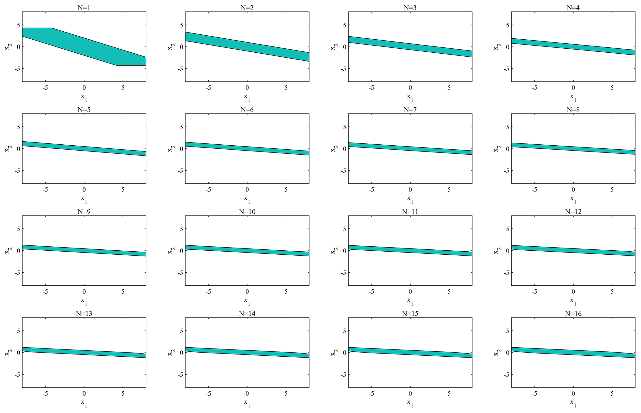
The N-step controllable set can be derived, as shown in Fig. 5, using either the improved ESP algorithm or the original ESP algorithm. When N is small, the region of the N-step controllable set changes significantly with the increasing N, though the trend of change gradually weakens and when N≥12. The N-step controllable set no longer changes with the increase in N.

Figure 5 Results of the N-step controllable set.

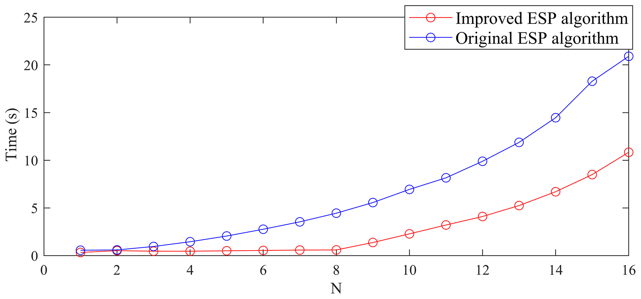
Moreover, the running times of the original ESP and the improved ESP are shown in Fig. 6. When $N=\mathrm{1},\mathrm{2}$, the two algorithms have similar computational efficiencies. When N>2, the computational efficiency of the improved ESP method is higher than that of the original ESP method. This is due to the fact that, when $N=\mathrm{1},\mathrm{2}$, dual degeneracy does not occur or occurs very rarely, while, when N>3, dual degeneracy occurs frequently. Clearly, the improved ESP algorithm is better than the original ESP method in the application of N-step controllable set computation.

Figure 6 Comparative running times for the calculation of the N-step controllable set.

6 Conclusions

In this paper, the improved ESP algorithm becomes simpler, faster, and easier to implement in the case of dual degeneracy. This is achieved by the following methods. First, an alternative criterion has been proposed to directly obtain the equality set that maximizes the value of $\text{dim}{P}_{E_f}$. It avoids the uniqueness discussion of the optimizer in linear programming, which is not easy to implement. Further, it also reduces the operation times and simplifies the algorithm process. Second, an improved strategy has been presented to solve the difficulty in searching for the equality set E_r in the case of $\text{dim}{P}_{E_f}>d-\mathrm{1}$, which significantly reduces the burden of computation. Finally, the effectiveness of the proposed improved ESP algorithm has been validated through numerical simulations.