A Lie group variational integrator in a closed-loop vector space without a multiplier

As a non-tree multi-body system, the dynamics model of four-bar mechanism is a differential algebraic equation. The constraints breach problem leads to many problems for computation accuracy and efficiency. With the traditional method, constructing an ODE-type dynamics equation for it is difficult or impossible. In this exploration, the dynamics model is built with geometry mechanic theory. The kinematic constraint variation relation of a closed-loop system is built in matrix and vector space with Lie group and Lie algebra theory respectively. The results indicate that the attitude variation between the driven body and the follower body has a linear recursion relation, which is the basis for dynamics modelling. With the Lie group variational integrator method, the closed-loop system Lagrangian dynamics model is built in vector space, with Legendre transformation. The dynamics model is reduced to be the Hamilton type. The kinematic model and dynamics model are solved using Newton iteration and the Runge–Kutta method respectively. As a special case of a crank and rocker mechanism, the dynamics character of a parallelogram mechanism is presented to verify the good structure conservation character of the closed-loop geometry dynamics model.

1 Introduction

As a non-tree multi-body system, the dynamics modelling and calculation of parallel mechanisms are widely employed, which is important for their design and analysis. As the most typical case of a parallel mechanism, the exploration of dynamics modelling and calculation of four-rod mechanisms has a great significance for representation. Traditionally, the Lagrange multiplier is used in the dynamics modelling of parallel mechanisms, which can add a constraint to the dynamics equation. To avoid the divergence of calculations, the algorithm needs to be carefully designed.

In recent years, the development of computation geometry gives a new solution to the dynamics problem of a parallel mechanism. The geometry method uses the Lie group and Lie algebra as a basis for dynamics modelling; the variation method is used for derivation, which can lead to a reduction during calculation. The geometry method can effectively reduce the complexity of the dynamics equation, which offers a new road to the enhancement of accuracy and efficiency.

In recent years, different kinds of methods have been used for dynamics modelling and analysis, such as the spinor method, the virtual principle, and the Newton–Euler method. Problems include singularity, inverse dynamics and forward kinematics. For example, with the spinor method, the singularity of a parallel mechanism is discussed, and the inverse dynamics model was built using the Lagrange equation (Zou and Zhang, 2021). The forward-inverse kinematics relation and dynamic relation are derived using geometry constraints, and the dynamics model is built using the virtual work principle (Lin, 2016). With the virtual principle, the dynamics model of a parallel mechanism can also be built (Rong, 2019; Wang, 2017; Chen and Liang, 2015). The inverse dynamics problem of a parallel mechanism can also be solved with the recursion-explicit algorithm (Staicu, 2015). The Newton–Euler method was used in dynamics modelling of a four-degrees-of-freedom parallel mechanism, and the driving force, momentum and constraint momentum were obtained (Wang et al., 2010).

In addition to the classic methods, the multi-body dynamics method was also used in compliant mechanism dynamics modelling, which is convenient for the design and operation of coupling problems (Van der Deijl and De Klerk, 2019). The dynamics model of the Stewart parallel mechanism is built using the linear transfer matrix of a multi-body system, and the mechanism seems to be a soft multi-body system, which is solved using the linear algebra method and modal superposition (Chen and Rui, 2018). With the Lagrange multiplier method, i.e. the dynamics model of a parallel mechanism in space with a multi-ball joint, the kinematic model is used to be the constraint in this method (Chen and Sun, 2019). A hierarchy method for the dynamics modelling of a parallel mechanism was designed using the modular modelling method (Hess-Coelho and Orsino, 2021). Using the centroid and momentum conservation method to build the displacement, velocity and acceleration of a parallel mechanism, the parameters of other parts are obtained using the superposition principle (Qi and Song, 2018). The dynamics model of a rigid–flexible coupling parallel mechanism can also be built using the natural coordinate and absolute nodal coordinate methods. The inverse multi-body dynamics model is built using the Lagrange method and solved using the generalized α method (Shi et al., 2019). The floating coordinate and Lagrange method is used to build a rigid–flexible coupling dynamics model of a satellite antenna's parallel mechanism (Zhang and Song, 2021). The inverse Lagrange dynamics model of a bionic underwater robot's parallel mechanism is built (Algarin-Pinto and Garza-Castanon, 2021). There are two types of dynamics model of a parallel mechanism, which has a reduced number of parameters. So the model is simplified, and the amount of calculation is also reduced (Abeywardena and Chen, 2017).

In the aspect of geometry kinematics and dynamics modelling of a parallel mechanism, the Lie group and Lie algebra methods are widely used, which can make the kinematics and dynamics model compact. With Lie group theory and the Cayley map between the Lie group and Lie algebra, the high-order relative kinematics model, the exact closed-form solutions of the motion in a non-inertial reference frame, and the minimal parameterization of rigid-body displacement and motion are explored, which offers a convenient tool for the kinematic analysis of a complex parallel mechanism in space (Condurache and Sfartz, 2021; Condurache, 2022; Condurache and Popa, 2023). The motion of each branch of a parallel mechanism was expressed with Lie group theory (Ye and Fang, 2016), and the transformation and spinor differential calculation of a mechanism in space was also solved with the Lie group and Lie algebra theory. With Lie group theory, the kinematics analysis for a parallel mechanism, which includes the Jacobian and Hessian matrix of a closed-loop mechanism, are built (Sun et al., 2021). With spinor theory and Lie group theory, the higher derivative of closed-loop equation was researched (Muller and Herder, 2019). The structure problem of a parallel mechanism was solved with Lie group theory (Rybak et al., 2017). The systematic analysis method for the multi-freedom driving system was built with Lie group theory (Li et al., 2020). A forward exact analysis method was used for the position error of a parallel mechanism under redundant drive with Lie group and spinor theory (Ding et al., 2019). Different types of series-parallel mixture connection mechanisms were built with the Lie group and an incidence matrix (Zeng and Fang, 2009). The kinematics model was built with Lie group theory, which is used to analyse and synthesize the mechanism (Wu et al., 2013). The screw system is closed under two continuous Lie bracket calculations. The definition of the whole Lie group trebling screw system is built with the Lie group and Lie algebra (Wu and Carricato, 2017). Sanchez-Garcia presented a method to define the motion of a parallel mechanism based on the concept of screw theory, the Lie group and a special Euclid group (Sanchez-Garcia et al., 2021). With the geometry analysis method, the inertia parameters are clustered and the number of parameters is reduced, which is convenient for the enhancement of efficiency and accuracy of the calculation (Danaei et al., 2017). With the absolute nodal coordinate method, the dynamics model of a parallel mechanism was built, and the relation of rigid and flexible bodies was built using the tangent coordinate (Wang and Liu, 2018).

According to the above analysis, in the domain of parallel-mechanism dynamics modelling, the virtual work principle is the main tool, and the dynamics model mainly uses the dynamic static solution. Based on the Lie group and Lie algebra theory and the rotation in a plane, a new type of expression, which is similar to the position vector, is presented in this paper. The variation relation of a closed loop is derived from the variation method, the dynamics model is built using the Lie group and the Lagrange method, and the model is changed to the Hamilton type with Legendre transformation. The dynamics model is finally changed to be a nonlinear equation and solved using Newton iteration.

2 Geometry dynamics modelling method

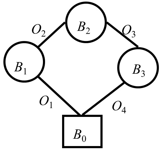
The four-bar mechanism is a type of non-tree structure. The topology of it is as shown in Fig. 1. B_i represents a rigid body, and O_i is the connection between rigid bodies which are assumed to be a revolute pair. In order to build the dynamics model, it is necessary to build the pose and attitude constraint of a closed loop. Usually, any O_i is cut open, which can transform the closed loop into two open loops. The positions of these two loops' end points satisfy the equality relation. Then the velocity and acceleration constraints can be derived based on pose and attitude constraints. Traditionally, the rotation relation between two rigid bodies can be expressed using a triangle function which has a complex expression. The Lie group method is used instead of it. See Fig. 1 for an example. Cutting the joint O₃ open, the system is changed to trees of $B_{\mathrm{0}}-B_{\mathrm{1}}-B_{\mathrm{2}}$ and B₀−B₃ respectively. They cross at point O₃.

Figure 1 Multi-body topology of a parallel mechanism.

The expression of the Lie group is as follows. Firstly, the rotation angle is used to express the rotation condition of two bodies. Suppose the rotation angle of the single freedom joint is θ. The rotation matrix R of the body can be obtained by exponential mapping, as in Eq. (1).

$$\begin{array}{}\text{(1)}& \mathbf{R}={\mathit{e}}^{\mathit{S}\left(\mathit{\theta }\right)}\end{array}$$

In Eq. (1), $\mathit{S}\left(\mathit{\theta }\right)=\left[\begin{array}{cc}\mathrm{0}& -\mathit{\theta }\\ \mathit{\theta }& \mathrm{0}\end{array}\right]$. R is the Lie group expression of rotation, and θ is Lie algebra corresponding to R. Make the differential of Eq. (1), and the result is as in Eq. (2).

$$\begin{array}{}\text{(2)}& \dot{\mathbf{R}}={\mathit{e}}^{\mathit{S}\left(\mathit{\theta }\right)}\mathit{S}\left(\dot{\mathit{\theta }}\right)=\mathit{\omega }\mathbf{R}{\mathit{S}}_{\mathrm{1}}\end{array}$$

Equation (2) shows angular velocity. Besides derivation, variation is the key tool of Lie group calculation. Applying variation to R, the result is as in Eq. (3).

$$\begin{array}{}\text{(3)}& \mathit{\delta }\mathbf{R}={\mathit{e}}^{\mathit{S}\left(\mathit{\theta }\right)}\mathit{S}\left(\mathit{\delta }\mathit{\theta }\right)\end{array}$$

Supposing that η=δθ, Eq. (3) can transform to be Eq. (4).

$$\begin{array}{}\text{(4)}& \mathit{\delta }\mathbf{R}=\mathit{\eta }\mathbf{R}{\mathit{S}}_{\mathrm{1}}\end{array}$$

The structure in Fig. 1 is used as an example to indicate the function of variation in dynamics modelling of a closed-loop mechanism. This structure satisfies the pose and attitude constraint as in Eq. (5).

$$\begin{array}{}\text{(5)}& {\mathbf{R}}_{\mathrm{1}}{\mathit{l}}_{\mathrm{1}}+{\mathbf{R}}_{\mathrm{2}}{\mathit{l}}_{\mathrm{2}}={\mathbf{R}}_{\mathrm{4}}{\mathit{l}}_{\mathrm{4}}\end{array}$$

Apply variation to Eq. (5), as in Eq. (6).

$$\begin{array}{}\text{(6)}& \mathit{\delta }{\mathbf{R}}_{\mathrm{1}}{\mathit{l}}_{\mathrm{1}}+\mathit{\delta }{\mathbf{R}}_{\mathrm{2}}{\mathit{l}}_{\mathrm{2}}=\mathit{\delta }{\mathbf{R}}_{\mathrm{4}}{\mathit{l}}_{\mathrm{4}}\end{array}$$

Substitute Eq. (4) into Eq. (6), and the result is as in Eq. (7).

$$\begin{array}{}\text{(7)}& {\mathit{\eta }}_{\mathrm{1}}{\mathbf{R}}_{\mathrm{1}}{\mathit{S}}_{\mathrm{1}}{\mathit{l}}_{\mathrm{1}}+{\mathit{\eta }}_{\mathrm{2}}{\mathbf{R}}_{\mathrm{2}}{\mathit{S}}_{\mathrm{1}}{\mathit{l}}_{\mathrm{2}}={\mathit{\eta }}_{\mathrm{4}}{\mathbf{R}}_{\mathrm{4}}{\mathit{S}}_{\mathrm{1}}{\mathit{l}}_{\mathrm{4}}\end{array}$$

Change Eq. (7) to be the matrix type as in Eq. (8).

$$\begin{array}{}\text{(8)}& \left[\begin{array}{l}{\mathit{\eta }}_{\mathrm{2}}\\ {\mathit{\eta }}_{\mathrm{4}}\end{array}\right]=-{\mathit{\eta }}_{\mathrm{1}}{\left[\begin{array}{cc}{\mathbf{R}}_{\mathrm{2}}{\mathit{S}}_{\mathrm{1}}{\mathit{l}}_{\mathrm{2}}& -{\mathbf{R}}_{\mathrm{4}}{\mathit{S}}_{\mathrm{1}}{\mathit{l}}_{\mathrm{4}}\end{array}\right]}^{-\mathrm{1}}{\mathbf{R}}_{\mathrm{1}}{\mathit{S}}_{\mathrm{1}}{\mathit{l}}_{\mathrm{1}}\end{array}$$

The constraint relation of a closed-loop system is obtained by variation, which is important in dynamics derivation. In the following, the dynamics modelling process is discussed as follows. The Lagrange function is built first, which is the function of angular velocity and the rotation matrix: $L=L\left(\mathbf{R},\mathit{\omega }\right)$. Apply variation to it with respect to angular velocity, as in Eq. (9).

$$\begin{array}{}\text{(9)}& {\mathit{\delta }}_{\mathit{\omega }}L={\mathbf{D}}_{\mathit{\omega }}L\left(\mathbf{R},\mathit{\omega }\right)\cdot \mathit{\delta }\mathit{\omega }\end{array}$$

According to Hamilton theory, the variation in the Lagrange function with respect to angular velocity is equal to momentum, as in Eq. (10).

$$\begin{array}{}\text{(10)}& \mathbf{\Pi }={\mathbf{D}}_{\mathit{\omega }}L\left(\mathbf{R},\mathit{\omega }\right)\end{array}$$

Applying derivation to Eq. (10), the inertia moment with respect to the momentum in Eq. (10) can be obtained. Except for the inertia moment, the moment of motion also includes coupling of angular velocity and momentum, as in Eq. (11).

$$\begin{array}{}\text{(11)}& {\mathrm{ad}}_{\mathit{\omega }}^{\ast }\cdot {\mathbf{D}}_{\mathit{\omega }}L\left(\mathbf{R},\mathit{\omega }\right)=\mathit{S}\left(\mathit{\omega }\right)\cdot {\mathbf{D}}_{\mathit{\omega }}L\left(\mathbf{R},\mathit{\omega }\right)\end{array}$$

For the single freedom joint, the coupling part is 0, as in Eq. (12).

$$\begin{array}{}\text{(12)}& {\mathrm{ad}}_{\mathit{\omega }}^{\ast }\cdot {\mathbf{D}}_{\mathit{\omega }}L\left(\mathbf{R},\mathit{\omega }\right)=\mathrm{0}\end{array}$$

The inertia moment, which is deduced by potential, is as follows. Applying variation to Lagrange function with respect to attitude matrix R, the result is as in Eq. (13).

$$\begin{array}{}\text{(13)}& {\mathit{\delta }}_{R}L={\mathbf{D}}_{R}L\left(\mathbf{R},\mathit{\omega }\right)\cdot \mathit{\eta }\end{array}$$

In Eq. (13), D_RL(R,ω) is a row vector; apply transposition to it, and the tangent of Eq. (13) is as in Eq. (14).

$$\begin{array}{}\text{(14)}& {\mathbf{T}}_e^{\ast }{\mathbf{L}}_R\cdot {\mathbf{D}}_{R}L\left(\mathbf{R},\mathit{\omega }\right)={\left({\mathbf{D}}_{R}L\left(\mathbf{R},\mathit{\omega }\right)\right)}^T\end{array}$$

The dynamics equation is as in Eq. (15).

$$\begin{array}{}\text{(15)}& \begin{array}{rl}{\displaystyle \frac{\mathrm{d}}{\mathrm{d}t}}& {\mathbf{D}}_{\mathit{\omega }}L\left(\mathbf{R},\mathit{\omega }\right)-{\mathbf{ad}}_{\mathit{\omega }}^{\ast }\cdot {\mathbf{D}}_{\mathit{\omega }}L\left(\mathbf{R},\mathit{\omega }\right)-{\mathbf{T}}_e^{\ast }{L}_R\\ & \cdot {\mathbf{D}}_{R}L\left(\mathbf{R},\mathit{\omega }\right)=\mathrm{0}\end{array}\end{array}$$

If the system is in a plane, the simplified dynamics equation is as in Eq. (16).

$$\begin{array}{}\text{(16)}& {\displaystyle \frac{\mathrm{d}}{\mathrm{d}t}}{\mathbf{D}}_{\mathit{\omega }}L\left(\mathbf{R},\mathit{\omega }\right)-{\mathbf{T}}_e^{\ast }{L}_R\cdot {\mathbf{D}}_{R}L\left(\mathbf{R},\mathit{\omega }\right)=\mathrm{0}\end{array}$$

According to Eq. (10), Eq. (16) can be transformed to the Hamilton dynamics equation using Legendre transformation as in Eq. (17).

$$\begin{array}{}\text{(17)}& \dot{\mathbf{\Pi }}-{\mathrm{ad}}_{\mathit{\omega }}^{\ast }\mathbf{\Pi }-{\mathbf{T}}_e^{\ast }{L}_{\mathbf{g}}\cdot {\mathbf{D}}_{R}L\left(\mathbf{R},\mathit{\omega }\right)=\mathrm{0}\end{array}$$

In addition to the rotation matrix, the attitude vector can express the rotation between rigid bodies too. The relation between the attitude matrix and vector is as in Eq. (18).

$$\begin{array}{}\text{(18)}& \mathit{q}=\mathit{R}{\mathit{e}}_{\mathrm{1}}\end{array}$$

Apply derivation to Eq. 18), as in Eq. (19).

$$\begin{array}{}\text{(19)}& \dot{\mathbf{q}}=\dot{\mathbf{R}}{\mathbf{e}}_{\mathrm{1}}=\mathit{\omega }{\mathbf{RS}}_{\mathrm{1}}{\mathit{e}}_{\mathrm{1}}=\mathit{\omega }\mathit{R}{\mathit{e}}_{\mathrm{2}}=\mathit{\omega }{\mathit{S}}_{\mathrm{1}}\mathit{q}\end{array}$$

The variation calculation also satisfies a similar process to the one in Eq. (20).

$$\begin{array}{}\text{(20)}& \mathit{\delta }\mathit{q}=\mathit{\eta }{\mathit{S}}_{\mathrm{1}}\mathit{q}\end{array}$$

3 Kinematic analysis of four-bar mechanism

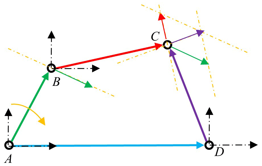
Figure 2 is the sketch map of a four-bar mechanism. Suppose that the lengths of bar AB, BC, CD and AD are l₁, l₂, l₃ and l₄ respectively. The rotation angles of bar AB, BC and CD are θ_A, θ_B and θ_D respectively. Define the initial position of each rod coinciding with the horizontal axis, and the direction of rotation is anti-clockwise. The closed-loop mechanism has three constraints on pose and attitude, velocity, and acceleration respectively. They are built using differential calculations, which means that the velocity constraint is obtained by applying derivation to the pose–attitude constraint, and the acceleration constraint is obtained by derivation from velocity. Suppose the rotation matrixes of AB, BC and CD are R_A, R_B and R_D respectively. The pose–attitude constraint is as in Eq. (21).

$$\begin{array}{}\text{(21)}& l_{\mathrm{2}}{\mathbf{R}}_B{\mathit{e}}_{\mathrm{1}}-l_{\mathrm{3}}{\mathbf{R}}_D{\mathit{e}}_{\mathrm{1}}=-l_{\mathrm{1}}{\mathbf{R}}_A{\mathit{e}}_{\mathrm{1}}+l_{\mathrm{4}}{\mathit{e}}_{\mathrm{1}}\end{array}$$

Figure 2 The four-bar mechanism.

In Eq. (21), e₁ is unit vector: ${\mathit{e}}_{\mathrm{1}}=\left[\mathrm{1};\mathrm{0}\right]$. Applying derivation to Eq. (21), the velocity constraint is as in Eq. (22).

$$\begin{array}{}\text{(22)}& {\mathit{\omega }}_B{l}_{\mathrm{2}}{\mathbf{R}}_B{\mathit{e}}_{\mathrm{2}}-{\mathit{\omega }}_D{l}_{\mathrm{3}}{\mathbf{R}}_D{\mathit{e}}_{\mathrm{2}}=-{\mathit{\omega }}_A{l}_{\mathrm{1}}{\mathbf{R}}_A{\mathit{e}}_{\mathrm{2}}\end{array}$$

In Eq. (22), ω_A, ω_B and ω_D are angular velocities of AB, BC and CD respectively. Apply derivation to Eq. (22), and the acceleration constraint is as in Eq. (23).

$$\begin{array}{}\text{(23)}& \begin{array}{rl}{\mathit{\alpha }}_B{l}_{\mathrm{2}}& {\mathbf{R}}_B{\mathit{e}}_{\mathrm{2}}-{\mathit{\alpha }}_D{l}_{\mathrm{3}}{\mathbf{R}}_D{\mathit{e}}_{\mathrm{2}}=-{\mathit{\alpha }}_A{l}_{\mathrm{1}}{\mathbf{R}}_A{\mathit{e}}_{\mathrm{2}}-{\mathit{\omega }}_A^{\mathrm{2}}{l}_{\mathrm{1}}{\mathbf{R}}_A{\mathit{e}}_{\mathrm{1}}\\ & +{\mathit{\omega }}_B^{\mathrm{2}}{l}_{\mathrm{2}}{\mathbf{R}}_B{\mathit{e}}_{\mathrm{1}}-{\mathit{\omega }}_D^{\mathrm{2}}{l}_{\mathrm{3}}{\mathbf{R}}_D{\mathit{e}}_{\mathrm{1}}\end{array}\end{array}$$

In Eq. (23), α_A, α_B and α_D are angular velocities of AB, BC and CD respectively. In Eq. (21) to Eq. (23), the attitudes are expressed by rotation matrixes, and the rotation matrixes can be simplified to be the vectors accord to Eq. (18). Define the relation of the rotation matrix and vector as in Eq. (24).

$$\begin{array}{}\text{(24)}& \left\{\begin{array}{l}{\mathit{q}}_A={\mathbf{R}}_A{\mathit{e}}_{\mathrm{1}}\\ {\mathit{q}}_B={\mathbf{R}}_B{\mathit{e}}_{\mathrm{1}}\\ {\mathit{q}}_D={\mathbf{R}}_D{\mathit{e}}_{\mathrm{1}}\end{array}\right.\end{array}$$

Substitute Eq. (24) into Eq. (21). The pose–attitude constraint based on the direction vector is obtained as in Eq. (25).

$$\begin{array}{}\text{(25)}& l_{\mathrm{2}}{\mathit{q}}_B-l_{\mathrm{3}}{\mathit{q}}_D+l_{\mathrm{1}}{\mathit{q}}_A-l_{\mathrm{4}}{\mathit{e}}_{\mathrm{1}}={\mathbf{0}}_{\mathrm{2}\times \mathrm{1}}\end{array}$$

Applying derivation to Eq. (25), the velocity constraint is as in Eq. (26).

$$\begin{array}{}\text{(26)}& {\mathit{\omega }}_B{l}_{\mathrm{2}}{\mathit{S}}_{\mathrm{1}}{\mathit{q}}_B-{\mathit{\omega }}_D{l}_{\mathrm{3}}{\mathit{S}}_{\mathrm{1}}{\mathit{q}}_D=-{\mathit{\omega }}_A{l}_{\mathrm{1}}{\mathit{S}}_{\mathrm{1}}{\mathit{q}}_A\end{array}$$

Transform the velocity constraint to the matrix type as in Eq. (27).

$$\begin{array}{}\text{(27)}& \left[\begin{array}{l}{\mathit{\omega }}_{\mathrm{2}}\\ {\mathit{\omega }}_D\end{array}\right]=-{\mathit{\omega }}_A{\left[l_{\mathrm{2}}{\mathit{S}}_{\mathrm{1}}{\mathit{q}}_B,-l_{\mathrm{3}}{\mathit{S}}_{\mathrm{1}}{\mathit{q}}_D\right]}^{-\mathrm{1}}{l}_{\mathrm{1}}{\mathit{S}}_{\mathrm{1}}{\mathit{q}}_A\end{array}$$

As in Eq. (26), the left and right parts are multiplied by the skew matrix, S₁. Reduce S₁, and the velocity constraint changes to be as in Eq. (28).

$$\begin{array}{}\text{(28)}& {\mathit{\omega }}_B{l}_{\mathrm{2}}{\mathit{q}}_B-{\mathit{\omega }}_D{l}_{\mathrm{3}}{\mathit{q}}_D=-{\mathit{\omega }}_A{l}_{\mathrm{1}}{\mathit{q}}_A\end{array}$$

The constraint of acceleration is as in Eq. (29) by applying derivation to Eq. (28).

$$\begin{array}{}\text{(29)}& \begin{array}{rl}{\mathit{\alpha }}_B{l}_{\mathrm{2}}& {\mathit{S}}_{\mathrm{1}}{\mathit{q}}_B-{\mathit{\alpha }}_D{l}_{\mathrm{3}}{\mathit{S}}_{\mathrm{1}}{\mathit{q}}_D+{\mathit{\alpha }}_A{l}_{\mathrm{1}}{\mathit{S}}_{\mathrm{1}}{\mathit{q}}_A={\mathit{\omega }}_B^{\mathrm{2}}{l}_{\mathrm{2}}{\mathit{q}}_B\\ & -{\mathit{\omega }}_A^{\mathrm{2}}{l}_{\mathrm{1}}{\mathit{q}}_A-{\mathit{\omega }}_D^{\mathrm{2}}{l}_{\mathrm{3}}{\mathit{q}}_D\end{array}\end{array}$$

4 The variation and dynamics modelling

Based on kinematics model, the dynamics equation of a system can be obtained by variation of the Lagrange function. According to the pose–attitude constraint in Eq. (21), the variation of it is as in Eq. (30).

$$\begin{array}{}\text{(30)}& l_{\mathrm{2}}{\mathit{S}}_{\mathrm{1}}{\mathit{q}}_B{\mathit{\eta }}_B-l_{\mathrm{3}}{\mathit{S}}_{\mathrm{1}}{\mathit{q}}_D{\mathit{\eta }}_D=-l_{\mathrm{1}}{\mathit{S}}_{\mathrm{1}}{\mathit{q}}_A{\mathit{\eta }}_A\end{array}$$

Transform Eq. (30) to be a matrix type as in Eq. (31).

$$\begin{array}{}\text{(31)}& \left[\begin{array}{cc}{l}_{\mathrm{2}}{\mathit{S}}_{\mathrm{1}}{\mathit{q}}_B& -l_{\mathrm{3}}{\mathit{S}}_{\mathrm{1}}{\mathit{q}}_D\end{array}\right]\left[\begin{array}{l}{\mathit{\eta }}_B\\ {\mathit{\eta }}_D\end{array}\right]=-l_{\mathrm{1}}{\mathit{S}}_{\mathrm{1}}{\mathit{q}}_A{\mathit{\eta }}_A\end{array}$$

Apply inversion to the matrix in Eq. (31). The relation between η_B, η_D and η_A is as in Eq. (32).

$$\begin{array}{}\text{(32)}& \left[\begin{array}{l}{\mathit{\eta }}_B\\ {\mathit{\eta }}_D\end{array}\right]=-l_{\mathrm{1}}{\left[\begin{array}{cc}{l}_{\mathrm{2}}{\mathit{S}}_{\mathrm{1}}{\mathit{q}}_B& -l_{\mathrm{3}}{\mathit{S}}_{\mathrm{1}}{\mathit{q}}_D\end{array}\right]}^{-\mathrm{1}}{\mathit{S}}_{\mathrm{1}}{\mathit{q}}_A{\mathit{\eta }}_A\end{array}$$

If the inverse matrix in Eq. (32) is a 2×2 matrix, it can be solved directly. The inverse calculation is expressed by a triangle functions, as in Eq. (33).

$$\begin{array}{}\text{(33)}& \begin{array}{rl}& {\left[l_{\mathrm{2}}{\mathit{S}}_{\mathrm{1}}{\mathit{q}}_B,-l_{\mathrm{3}}{\mathit{S}}_{\mathrm{1}}{\mathit{q}}_D\right]}^{-\mathrm{1}}=\left[\begin{array}{cc}-l_{\mathrm{2}}\sin {\mathit{\theta }}_B& l_{\mathrm{3}}\sin {\mathit{\theta }}_D\\ l_{\mathrm{2}}\cos {\mathit{\theta }}_B& -l_{\mathrm{3}}\cos {\mathit{\theta }}_D\end{array}\right]\\ & ={\displaystyle \frac{\mathrm{1}}{l_{\mathrm{2}}{l}_{\mathrm{3}}\sin \left({\mathit{\theta }}_D-{\mathit{\theta }}_B\right)}}\left[\begin{array}{cc}{l}_{\mathrm{3}}\cos {\mathit{\theta }}_D& l_{\mathrm{3}}\sin {\mathit{\theta }}_D\\ l_{\mathrm{2}}\cos {\mathit{\theta }}_B& l_{\mathrm{2}}\sin {\mathit{\theta }}_B\end{array}\right]\\ & ={\displaystyle \frac{\mathrm{1}}{l_{\mathrm{2}}{l}_{\mathrm{3}}{\mathit{q}}_D^T{\mathit{S}}_{\mathrm{1}}{\mathit{q}}_B}}\left[l_{\mathrm{3}}{\mathit{q}}_D^T;l_{\mathrm{2}}{\mathit{q}}_B^T\right]\end{array}\end{array}$$

Substitute Eq. (33) into Eq. (32), the result is as in Eq. (34).

$$\begin{array}{}\text{(34)}& \left[\begin{array}{l}{\mathit{\eta }}_B\\ {\mathit{\eta }}_D\end{array}\right]={\displaystyle \frac{-l_{\mathrm{1}}}{l_{\mathrm{2}}{l}_{\mathrm{3}}{\mathit{q}}_D^T{\mathit{S}}_{\mathrm{1}}{\mathit{q}}_B}}\left[\begin{array}{l}{l}_{\mathrm{3}}{\mathit{q}}_D^T{\mathit{S}}_{\mathrm{1}}{\mathit{q}}_A\\ l_{\mathrm{2}}{\mathit{q}}_B^T{\mathit{S}}_{\mathrm{1}}{\mathit{q}}_A\end{array}\right]{\mathit{\eta }}_A\end{array}$$

According to the above analysis, the variation relation of the attitude matrix of the rocker and the link can be expressed by the variation in crank under the constraint of pose and attitude. Comparing Eqs. (27) and (32), they have the uniform expressions. We define the same part of Eqs. (27) and (32) as Eq. (35).

$$\begin{array}{}\text{(35)}& \mathit{K}={\displaystyle \frac{-l_{\mathrm{1}}}{l_{\mathrm{2}}{l}_{\mathrm{3}}{\mathit{q}}_D^T{\mathit{S}}_{\mathrm{1}}{\mathit{q}}_B}}\left[\begin{array}{l}{l}_{\mathrm{3}}{\mathit{q}}_D^T{\mathit{S}}_{\mathrm{1}}{\mathit{q}}_A\\ l_{\mathrm{2}}{\mathit{q}}_B^T{\mathit{S}}_{\mathrm{1}}{\mathit{q}}_A\end{array}\right]\end{array}$$

The velocity constraint satisfies the relation as in Eq. (36).

$$\begin{array}{}\text{(36)}& \left[\begin{array}{l}{\mathit{\omega }}_{\mathrm{2}}\\ {\mathit{\omega }}_D\end{array}\right]=\mathit{K}{\mathit{\omega }}_A\end{array}$$

The dynamics model of a system is derived as follows. Supposing the masses of rod AB, BC and CD are m₁, m₂ and m₃ respectively. Their position vectors are ρ₁, ρ₂, ρ₃ respectively. Their rotational inertia is J₁, J₂ and J₃ respectively.

The kinetics of each part in the mechanism consist of the rotation kinetics along the mass centre and the translational kinetics of centre of mass. The displacement of the mass centre of AB is as in Eq. (37).

$$\begin{array}{}\text{(37)}& {\mathit{l}}_{\mathrm{1}}={\mathit{q}}_A{\mathit{\rho }}_{\mathrm{1}x}+{\mathit{S}}_{\mathrm{1}}{\mathit{q}}_A{\mathit{\rho }}_{\mathrm{1}y}=\left({\mathit{\rho }}_{\mathrm{1}x}\mathit{I}+{\mathit{S}}_{\mathrm{1}}{\mathit{\rho }}_{\mathrm{1}y}\right){\mathit{q}}_A={\mathbf{\Gamma }}_{\mathrm{1}}{\mathit{q}}_A\end{array}$$

The velocity of it is as in Eq. (38) according to the derivation to Eq. (37).

$$\begin{array}{}\text{(38)}& {\mathit{v}}_{\mathrm{1}}={\mathit{\omega }}_{\mathrm{1}}{\mathbf{\Gamma }}_{\mathrm{1}}{\mathit{S}}_{\mathrm{1}}{\mathit{q}}_A\end{array}$$

In order to conserve the form of q_A, the position of the mass centre can change to be the matrix type, as in Eq. (39).

$$\begin{array}{}\text{(39)}& {\mathbf{\Gamma }}_{\mathrm{1}}={\mathit{\rho }}_{\mathrm{1}x}\mathit{I}+{\mathit{S}}_{\mathrm{1}}{\mathit{\rho }}_{\mathrm{1}y}=\left[\begin{array}{cc}{\mathit{\rho }}_{\mathrm{1}x}& -{\mathit{\rho }}_{\mathrm{1}y}\\ {\mathit{\rho }}_{\mathrm{1}y}& {\mathit{\rho }}_{\mathrm{1}x}\end{array}\right]\end{array}$$

Similarly, ρ₂, ρ₃ can also be expressed as in Eq. (40).

$$\begin{array}{}\text{(40)}& {\mathbf{\Gamma }}_{\mathrm{2}}=\left[\begin{array}{cc}{\mathit{\rho }}_{\mathrm{2}x}& -{\mathit{\rho }}_{\mathrm{2}y}\\ {\mathit{\rho }}_{\mathrm{2}y}& {\mathit{\rho }}_{\mathrm{2}x}\end{array}\right],{\mathbf{\Gamma }}_{\mathrm{3}}=\left[\begin{array}{cc}{\mathit{\rho }}_{\mathrm{3}x}& -{\mathit{\rho }}_{\mathrm{3}y}\\ {\mathit{\rho }}_{\mathrm{3}y}& {\mathit{\rho }}_{\mathrm{3}x}\end{array}\right]\end{array}$$

The displacement of the mass centre of BC is as in Eq. (41).

$$\begin{array}{}\text{(41)}& {\mathit{l}}_{\mathrm{2}}=l_{\mathrm{1}}{\mathit{q}}_A+{\mathbf{\Gamma }}_{\mathrm{2}}{\mathit{q}}_B\end{array}$$

The velocity of the mass centre is as in Eq. (42).

$$\begin{array}{}\text{(42)}& {\mathit{v}}_{\mathrm{2}}={\mathit{\omega }}_{\mathrm{1}}{l}_{\mathrm{1}}{\mathit{S}}_{\mathrm{1}}{\mathit{q}}_A+{\mathit{\omega }}_{\mathrm{2}}{\mathbf{\Gamma }}_{\mathrm{2}}{\mathit{S}}_{\mathrm{1}}{\mathit{q}}_B\end{array}$$

The angular velocity of CD is ω₃, so the position vector of the mass centre is as in Eq. (43).

$$\begin{array}{}\text{(43)}& {\mathit{l}}_{\mathrm{3}}=l_{\mathrm{4}}{\mathit{e}}_{\mathrm{1}}+{\mathbf{\Gamma }}_{\mathrm{3}}{\mathit{q}}_D\end{array}$$

The velocity of the mass centre is as in Eq. (44).

$$\begin{array}{}\text{(44)}& {\mathit{v}}_{\mathrm{3}}={\mathit{\omega }}_{\mathrm{3}}{\mathbf{\Gamma }}_{\mathrm{3}}{\mathit{S}}_{\mathrm{1}}{\mathit{q}}_D\end{array}$$

In order to make the expressions simple, the above equations are synthesized to be the matrix types. Suppose the angular velocity of a system is $\mathit{\omega }=\left[{\mathit{\omega }}_{\mathrm{1}};{\mathit{\omega }}_{\mathrm{2}};{\mathit{\omega }}_{\mathrm{3}}\right]$, the expression of it is as in Eq. (45).

$$\begin{array}{}\text{(45)}& \mathit{\omega }={\left[\begin{array}{cc}\mathrm{1}& \mathit{K}\end{array}\right]}^T{\mathit{\omega }}_{\mathrm{1}}\end{array}$$

Supposing $\mathit{l}=\left[{\mathit{l}}_{\mathrm{1}};{\mathit{l}}_{\mathrm{2}};{\mathit{l}}_{\mathrm{3}}\right]$, $\mathit{q}=\left[{\mathit{q}}_A;{\mathit{q}}_B;{\mathit{q}}_D\right]$, the displacements of the mass centre of the system can be written as the matrix type, as in Eq. (46).

$$\begin{array}{}\text{(46)}& \mathit{l}={\mathit{Z}}_{\mathrm{1}}\mathit{q}+{\mathbf{z}}_{\mathrm{1}}\end{array}$$

The parameters in Eq. (46) are as follows:

$${\mathit{Z}}_{\mathrm{1}}=\left[\begin{array}{ccc}{\mathbf{\Gamma }}_{\mathrm{1}}& {\mathit{I}}_{\mathrm{2}}& {\mathit{I}}_{\mathrm{2}}\\ l_{\mathrm{1}}{\mathit{I}}_{\mathrm{2}}& {\mathbf{\Gamma }}_{\mathrm{2}}& {\mathit{I}}_{\mathrm{2}}\\ {\mathit{I}}_{\mathrm{2}}& {\mathit{I}}_{\mathrm{2}}& {\mathbf{\Gamma }}_{\mathrm{3}}\end{array}\right],{\mathbf{z}}_{\mathrm{1}}=\left[\begin{array}{l}{\mathbf{0}}_{\mathrm{2}\times \mathrm{1}}\\ {\mathbf{0}}_{\mathrm{2}\times \mathrm{1}}\\ l_{\mathrm{4}}{\mathit{e}}_{\mathrm{1}}\end{array}\right].$$

Suppose $\mathit{v}=\left[{\mathit{v}}_{\mathrm{1}};{\mathit{v}}_{\mathrm{2}};{\mathit{v}}_{\mathrm{3}}\right]$. The velocity of the mass centre of the system is as in Eq. (47).

$$\begin{array}{}\text{(47)}& \mathit{v}=\dot{\mathit{l}}={\mathit{Z}}_{\mathrm{1}}\dot{\mathit{q}}\end{array}$$

The expression of $\dot{\mathbf{q}}$ is as equation Eq. (48).

$$\begin{array}{}\text{(48)}& \dot{\mathit{q}}=\left[\begin{array}{l}{\dot{\mathit{q}}}_A\\ {\dot{\mathit{q}}}_B\\ {\dot{\mathit{q}}}_D\end{array}\right]=\left[\begin{array}{l}{\mathit{\omega }}_A{\mathit{S}}_{\mathrm{1}}{\mathit{q}}_A\\ {\mathit{\omega }}_B{\mathit{S}}_{\mathrm{1}}{\mathit{q}}_B\\ {\mathit{\omega }}_D{\mathit{S}}_{\mathrm{1}}{\mathit{q}}_D\end{array}\right]={\mathit{Z}}_A\mathit{S}\mathit{q}\end{array}$$

The parameters in Eq. (48) are as follows:

$$\begin{array}{rl}& {\mathit{Z}}_A=\left[\begin{array}{ccc}{\mathit{\omega }}_A{\mathit{I}}_{\mathrm{2}\times \mathrm{2}}& {\mathbf{0}}_{\mathrm{2}\times \mathrm{2}}& {\mathbf{0}}_{\mathrm{2}\times \mathrm{2}}\\ {\mathbf{0}}_{\mathrm{2}\times \mathrm{2}}& {\mathit{\omega }}_B{\mathit{I}}_{\mathrm{2}\times \mathrm{2}}& {\mathbf{0}}_{\mathrm{2}\times \mathrm{2}}\\ {\mathbf{0}}_{\mathrm{2}\times \mathrm{2}}& {\mathbf{0}}_{\mathrm{2}\times \mathrm{2}}& {\mathit{\omega }}_D{\mathit{I}}_{\mathrm{2}\times \mathrm{2}}\end{array}\right],\\ & \mathbf{S}=\left[\begin{array}{ccc}{\mathit{S}}_{\mathrm{1}}& {\mathbf{0}}_{\mathrm{2}\times \mathrm{2}}& {\mathbf{0}}_{\mathrm{2}\times \mathrm{2}}\\ {\mathbf{0}}_{\mathrm{2}\times \mathrm{2}}& {\mathit{S}}_{\mathrm{1}}& {\mathbf{0}}_{\mathrm{2}\times \mathrm{2}}\\ {\mathbf{0}}_{\mathrm{2}\times \mathrm{2}}& {\mathbf{0}}_{\mathrm{2}\times \mathrm{2}}& {\mathit{S}}_{\mathrm{1}}\end{array}\right].\end{array}$$

According to Eq. (36), Z_Acan be written as the following type, as in Eq. (49).

$$\begin{array}{}\text{(49)}& {\mathit{Z}}_A={\mathit{\omega }}_A{\mathit{Z}}_{\mathrm{2}}\end{array}$$

The parameter in Eq. (49) is as follows:

$${\mathit{Z}}_{\mathrm{2}}=\left[\begin{array}{ccc}{\mathit{I}}_{\mathrm{2}\times \mathrm{2}}& {\mathbf{0}}_{\mathrm{2}\times \mathrm{2}}& {\mathbf{0}}_{\mathrm{2}\times \mathrm{2}}\\ {\mathbf{0}}_{\mathrm{2}\times \mathrm{2}}& {\mathit{e}}_{\mathrm{1}}^T\mathit{K}{\mathit{I}}_{\mathrm{2}\times \mathrm{2}}& {\mathbf{0}}_{\mathrm{2}\times \mathrm{2}}\\ {\mathbf{0}}_{\mathrm{2}\times \mathrm{2}}& {\mathbf{0}}_{\mathrm{2}\times \mathrm{2}}& {\mathit{e}}_{\mathrm{2}}^T\mathit{K}{\mathit{I}}_{\mathrm{2}\times \mathrm{2}}\end{array}\right].$$

Substitute Eq. (49) into Eq. (48), and the equation is changed to be the following type, as in Eq. (50).

$$\begin{array}{}\text{(50)}& \dot{\mathbf{q}}={\mathit{\omega }}_A{\mathit{Z}}_{\mathrm{2}}\mathit{S}\mathit{q}\end{array}$$

So the velocity of the mass centre is as in Eq. (51).

$$\begin{array}{}\text{(51)}& \mathit{v}=\dot{\mathbf{l}}={\mathit{\omega }}_A{\mathit{Z}}_{\mathrm{1}}{\mathit{Z}}_{\mathrm{2}}\mathit{S}\mathit{q}\end{array}$$

Then the kinetic and potential energy of the system are as in Eqs. (52) and (53) respectively.

$$\begin{array}{}\text{(52)}& \begin{array}{rl}& T={\displaystyle \frac{\mathrm{1}}{\mathrm{2}}}{\mathit{\omega }}^T\mathbf{J}\mathit{\omega }+{\displaystyle \frac{\mathrm{1}}{\mathrm{2}}}{\mathit{v}}^T\mathit{M}\mathit{v}\\ & ={\displaystyle \frac{\mathrm{1}}{\mathrm{2}}}{\left[\begin{array}{l}{\mathit{\omega }}_{\mathrm{1}}\\ {\mathit{\omega }}_{\mathrm{2}}\\ {\mathit{\omega }}_{\mathrm{3}}\end{array}\right]}^T\left[\begin{array}{ccc}{J}_{\mathrm{1}}& \mathrm{0}& \mathrm{0}\\ \mathrm{0}& J_{\mathrm{2}}& \mathrm{0}\\ \mathrm{0}& \mathrm{0}& J_{\mathrm{3}}\end{array}\right]\left[\begin{array}{l}{\mathit{\omega }}_{\mathrm{1}}\\ {\mathit{\omega }}_{\mathrm{2}}\\ {\mathit{\omega }}_{\mathrm{3}}\end{array}\right]\\ & +{\displaystyle \frac{\mathrm{1}}{\mathrm{2}}}{\left[\begin{array}{l}{\mathit{v}}_{\mathrm{1}}\\ {\mathit{v}}_{\mathrm{2}}\\ {\mathit{v}}_{\mathrm{3}}\end{array}\right]}^T\left[\begin{array}{ccc}{m}_{\mathrm{1}}\mathit{I}& {\mathbf{0}}_{\mathrm{2}\times \mathrm{2}}& {\mathbf{0}}_{\mathrm{2}\times \mathrm{2}}\\ {\mathbf{0}}_{\mathrm{2}\times \mathrm{2}}& m_{\mathrm{2}}\mathit{I}& {\mathbf{0}}_{\mathrm{2}\times \mathrm{2}}\\ {\mathbf{0}}_{\mathrm{2}\times \mathrm{2}}& {\mathbf{0}}_{\mathrm{2}\times \mathrm{2}}& m_{\mathrm{3}}\mathit{I}\end{array}\right]\left[\begin{array}{l}{\mathit{v}}_{\mathrm{1}}\\ {\mathit{v}}_{\mathrm{2}}\\ {\mathit{v}}_{\mathrm{3}}\end{array}\right]\end{array}\end{array}$$

$$\begin{array}{}\text{(53)}& \begin{array}{rl}V& =-g{\mathit{e}}_{\mathrm{2}}^T\left(m_{\mathrm{1}}{\mathit{l}}_{\mathrm{1}}+m_{\mathrm{2}}{\mathit{l}}_{\mathrm{2}}+m_{\mathrm{3}}{\mathit{l}}_{\mathrm{3}}\right)\\ & =-g{\left[\begin{array}{l}{\mathit{e}}_{\mathrm{2}}\\ {\mathit{e}}_{\mathrm{2}}\\ {\mathit{e}}_{\mathrm{2}}\end{array}\right]}^T\left[\begin{array}{ccc}{m}_{\mathrm{1}}\mathit{I}& {\mathbf{0}}_{\mathrm{2}\times \mathrm{2}}& {\mathbf{0}}_{\mathrm{2}\times \mathrm{2}}\\ {\mathbf{0}}_{\mathrm{2}\times \mathrm{2}}& m_{\mathrm{2}}\mathit{I}& {\mathbf{0}}_{\mathrm{2}\times \mathrm{2}}\\ {\mathbf{0}}_{\mathrm{2}\times \mathrm{2}}& {\mathbf{0}}_{\mathrm{2}\times \mathrm{2}}& m_{\mathrm{3}}\mathit{I}\end{array}\right]\left[\begin{array}{l}{\mathit{l}}_{\mathrm{1}}\\ {\mathit{l}}_{\mathrm{2}}\\ {\mathit{l}}_{\mathrm{3}}\end{array}\right]\\ & =-g{\mathit{E}}_{\mathrm{6}\times \mathrm{1}}\mathit{M}\mathit{l}\end{array}\end{array}$$

According to Eqs. (52) and (53), the Lagrange function of four-bar system is as in Eq. (54).

$$\begin{array}{}\text{(54)}& L={\displaystyle \frac{\mathrm{1}}{\mathrm{2}}}{\mathit{\omega }}^T\mathit{J}\mathit{\omega }+{\displaystyle \frac{\mathrm{1}}{\mathrm{2}}}{\mathit{v}}^T\mathit{M}\mathit{v}\mathbf{+}g{\mathit{E}}_{\mathrm{6}\times \mathrm{1}}\mathit{M}\mathit{l}\end{array}$$

Applying variation to Eq. (72) aboutω₁, the result is as in Eq. (55).

$$\begin{array}{}\text{(55)}& {\mathit{\delta }}_{{\mathit{\omega }}_{\mathrm{1}}}L={\mathit{\omega }}^T\mathit{J}\left({\mathit{\delta }}_{{\mathit{\omega }}_{\mathrm{1}}}\mathit{\omega }\right)+{\mathit{v}}^T\mathbf{M}\left({\mathit{\delta }}_{{\mathit{\omega }}_{\mathrm{1}}}\mathit{v}\right)\end{array}$$

Applying derivation to Eq. (55), the result is as in Eq. (56).

$$\begin{array}{}\text{(56)}& \begin{array}{rl}{\displaystyle \frac{\mathrm{d}}{\mathrm{d}t}}{\mathit{\delta }}_{{\mathit{\omega }}_{\mathrm{1}}}L& ={\dot{\mathit{\omega }}}^T\mathit{J}\left({\mathit{\delta }}_{{\mathit{\omega }}_{\mathrm{1}}}\mathit{\omega }\right)+{\mathit{\omega }}^T\mathit{J}{\displaystyle \frac{\mathbf{d}}{\mathbf{d}t}}\left({\mathit{\delta }}_{{\mathit{\omega }}_{\mathrm{1}}}\mathit{\omega }\right)\\ & +{\dot{\mathbf{v}}}^T\mathbf{M}\left({\mathit{\delta }}_{{\mathit{\omega }}_{\mathrm{1}}}\mathit{v}\right)+{\mathit{v}}^T\mathbf{M}{\displaystyle \frac{\mathbf{d}}{\mathbf{d}t}}\left({\mathit{\delta }}_{{\mathit{\omega }}_{\mathrm{1}}}\mathit{v}\right)\end{array}\end{array}$$

Applying variation to Eq. (54) to the attitude vector, the result is as in Eq. (57).

$$\begin{array}{}\text{(57)}& {\mathit{\delta }}_{{\mathit{\eta }}_{\mathrm{1}}}L={\mathit{\omega }}^T\mathit{J}\left({\mathit{\delta }}_{{\mathit{\eta }}_{\mathrm{1}}}\mathit{\omega }\right)+{\mathit{v}}^T\mathbf{M}\left({\mathit{\delta }}_{{\mathit{\eta }}_{\mathrm{1}}}\mathit{v}\right)+g{\mathit{E}}_{\mathrm{6}\times \mathrm{1}}\mathbf{M}\left({\mathit{\delta }}_{{\mathit{\eta }}_{\mathrm{1}}}\mathit{l}\right)\end{array}$$

Substitute it into the geometry dynamics equation, and the Lagrange dynamics equation is as in Eq. (58).

$$\begin{array}{}\text{(58)}& \begin{array}{rl}& {\dot{\mathit{\omega }}}^T\mathit{J}\left({\mathit{\delta }}_{{\mathit{\omega }}_{\mathrm{1}}}\mathit{\omega }\right)+{\mathit{\omega }}^T\mathit{J}\left({\displaystyle \frac{\mathrm{d}}{\mathrm{d}t}}\left({\mathit{\delta }}_{{\mathit{\omega }}_{\mathrm{1}}}\mathit{\omega }\right)-\left({\mathit{\delta }}_{{\mathit{\eta }}_{\mathrm{1}}}\mathit{\omega }\right)\right)+{\dot{\mathbf{v}}}^T\mathbf{M}\\ & \left({\mathit{\delta }}_{{\mathit{\omega }}_{\mathrm{1}}}\mathit{v}\right)+{\mathit{v}}^T\mathbf{M}\left({\displaystyle \frac{d}{dt}}\left({\mathit{\delta }}_{{\mathit{\omega }}_{\mathrm{1}}}\mathit{v}\right)-\left({\mathit{\delta }}_{{\mathit{\eta }}_{\mathrm{1}}}\mathit{v}\right)\right)\\ & -g{\mathit{E}}_{\mathrm{6}\times \mathrm{1}}\mathbf{M}\left({\mathit{\delta }}_{{\mathit{\eta }}_{\mathrm{1}}}\mathit{l}\right)=\mathrm{0}\end{array}\end{array}$$

Let ${\mathrm{\Pi }}_{\mathrm{1}}={\mathit{\delta }}_{{\mathit{\omega }}_{\mathrm{1}}}L={\mathit{\omega }}^T\mathit{J}\left({\mathit{\delta }}_{{\mathit{\omega }}_{\mathrm{1}}}\mathit{\omega }\right)+{\mathit{v}}^T\mathbf{M}\left({\mathit{\delta }}_{{\mathit{\omega }}_{\mathrm{1}}}\mathit{v}\right)$; then the geometry dynamics equation of Hamilton types is as in Eq. (59).

$$\begin{array}{}\text{(59)}& {\dot{\mathrm{\Pi }}}_{\mathrm{1}}-{\mathit{\omega }}^T\mathit{J}\left({\mathit{\delta }}_{{\mathit{\eta }}_{\mathrm{1}}}\mathit{\omega }\right)-{\mathit{v}}^T\mathbf{M}\left({\mathit{\delta }}_{{\mathit{\eta }}_{\mathrm{1}}}\mathit{v}\right)-g{\mathit{E}}_{\mathrm{6}\times \mathrm{1}}\mathbf{M}\left({\mathit{\delta }}_{{\mathit{\eta }}_{\mathrm{1}}}\mathit{l}\right)=\mathrm{0}\end{array}$$

The variation of ω,v about ω₁ is as in Eqs. (60) and (61).

$$\begin{array}{}\text{(60)}& {\mathit{\delta }}_{{\mathit{\omega }}_{\mathrm{1}}}\mathit{\omega }=\left[\begin{array}{c}\mathrm{1}\\ \mathit{K}\end{array}\right]\mathit{\delta }{\mathit{\omega }}_{\mathrm{1}}\end{array}$$

$$\begin{array}{}\text{(61)}& {\mathit{\delta }}_{{\mathit{\omega }}_{\mathrm{1}}}\mathit{v}={\mathit{Z}}_{\mathrm{1}}{\mathit{Z}}_{\mathrm{2}}\mathit{S}\mathit{q}\mathit{\delta }{\mathit{\omega }}_{\mathrm{1}}\end{array}$$

The variation in attitude vectors is as follows. Expressions of kinetic and potential energies, angular velocity, velocity and mass centre positions all include the attitude vector. Applying variation to ω for attitude, the result is as in Eq. (62).

$$\begin{array}{}\text{(62)}& {\mathit{\delta }}_{{\mathit{\eta }}_{\mathrm{1}}}\mathit{\omega }=\left[\begin{array}{c}\mathrm{0}\\ {\mathit{\delta }}_{\mathit{\eta }}\mathit{K}\end{array}\right]{\mathit{\omega }}_{\mathrm{1}}\end{array}$$

Then applying variation to velocity, the result is as in Eq. (63).

$$\begin{array}{}\text{(63)}& {\mathit{\delta }}_{{\mathit{\eta }}_{\mathrm{1}}}\mathit{v}={\mathit{\omega }}_{\mathrm{1}}\left({\mathit{Z}}_{\mathrm{1}}\left({\mathit{\delta }}_{{\mathit{\eta }}_{\mathrm{1}}}{\mathit{Z}}_{\mathrm{2}}\right)\mathit{S}\mathit{q}+{\mathit{Z}}_{\mathrm{1}}{\mathit{Z}}_{\mathrm{2}}\mathit{S}\left({\mathit{\delta }}_{{\mathit{\eta }}_{\mathrm{1}}}\mathit{q}\right)\right)\end{array}$$

Applying variation to l, the result is as in Eq. (64).

$$\begin{array}{}\text{(64)}& {\mathit{\delta }}_{{\mathit{\eta }}_{\mathrm{1}}}\mathit{l}={\mathit{Z}}_{\mathrm{1}}{\mathit{\delta }}_{{\mathit{\eta }}_{\mathrm{1}}}\mathit{q}\end{array}$$

The concrete calculations of ${\mathit{\delta }}_{{\mathit{\eta }}_{\mathrm{1}}}\mathit{q}$ and ${\mathit{\delta }}_{{\mathit{\eta }}_{\mathrm{1}}}{\mathit{Z}}_{\mathrm{2}}$ are as follows. Applying variation to q, the expression changes to a new type, for which the variation parameters are in the same vector, as in Eq. (65).

$$\begin{array}{}\text{(65)}& \begin{array}{rl}\mathit{\delta }\mathit{q}& =\left[\begin{array}{l}\mathit{\delta }{\mathit{q}}_A\\ \mathit{\delta }{\mathit{q}}_B\\ \mathit{\delta }{\mathit{q}}_D\end{array}\right]=\left[\begin{array}{l}{\mathit{\eta }}_A{\mathit{S}}_{\mathrm{1}}{\mathit{q}}_A\\ {\mathit{\eta }}_B{\mathit{S}}_{\mathrm{1}}{\mathit{q}}_B\\ {\mathit{\eta }}_D{\mathit{S}}_{\mathrm{1}}{\mathit{q}}_D\end{array}\right]\\ & =\left[\begin{array}{ccc}{\mathit{S}}_{\mathrm{1}}{\mathit{q}}_A& {\mathbf{0}}_{\mathrm{2}\times \mathrm{1}}& {\mathbf{0}}_{\mathrm{2}\times \mathrm{1}}\\ {\mathbf{0}}_{\mathrm{2}\times \mathrm{1}}& {\mathit{S}}_{\mathrm{1}}{\mathit{q}}_B& {\mathbf{0}}_{\mathrm{2}\times \mathrm{1}}\\ {\mathbf{0}}_{\mathrm{2}\times \mathrm{1}}& {\mathbf{0}}_{\mathrm{2}\times \mathrm{1}}& {\mathit{S}}_{\mathrm{1}}{\mathit{q}}_D\end{array}\right]\left[\begin{array}{l}{\mathit{\eta }}_A\\ {\mathit{\eta }}_B\\ {\mathit{\eta }}_D\end{array}\right]\end{array}\end{array}$$

According to Eq. (35), the variation vector is as in Eq. (66).

$$\begin{array}{}\text{(66)}& \left[\begin{array}{l}{\mathit{\eta }}_A\\ {\mathit{\eta }}_B\\ {\mathit{\eta }}_D\end{array}\right]=\left[\begin{array}{l}\mathrm{1}\\ \mathit{K}\end{array}\right]{\mathit{\eta }}_A\end{array}$$

Substitute Eq. (66) into Eq. (65), and the result is as in Eq. (67).

$$\begin{array}{}\text{(67)}& \begin{array}{rl}& \mathit{\delta }\mathit{q}=\left[\begin{array}{l}\mathit{\delta }{\mathit{q}}_A\\ \mathit{\delta }{\mathit{q}}_B\\ \mathit{\delta }{\mathit{q}}_D\end{array}\right]=\left[\begin{array}{l}{\mathit{\eta }}_A{\mathit{S}}_{\mathrm{1}}{\mathit{q}}_A\\ {\mathit{\eta }}_B{\mathit{S}}_{\mathrm{1}}{\mathit{q}}_B\\ {\mathit{\eta }}_D{\mathit{S}}_{\mathrm{1}}{\mathit{q}}_D\end{array}\right]\\ & =\left[\begin{array}{ccc}{\mathit{S}}_{\mathrm{1}}{\mathit{q}}_A& {\mathbf{0}}_{\mathrm{2}\times \mathrm{1}}& {\mathbf{0}}_{\mathrm{2}\times \mathrm{1}}\\ {\mathbf{0}}_{\mathrm{2}\times \mathrm{1}}& {\mathit{S}}_{\mathrm{1}}{\mathit{q}}_B& {\mathbf{0}}_{\mathrm{2}\times \mathrm{1}}\\ {\mathbf{0}}_{\mathrm{2}\times \mathrm{1}}& {\mathbf{0}}_{\mathrm{2}\times \mathrm{1}}& {\mathit{S}}_{\mathrm{1}}{\mathit{q}}_D\end{array}\right]\left[\begin{array}{l}\mathrm{1}\\ \mathit{K}\end{array}\right]{\mathit{\eta }}_A={\mathit{S}}_{\mathit{q}}{\mathit{K}}_N{\mathit{\eta }}_A\end{array}\end{array}$$

The expression of ${\mathit{\delta }}_{{\mathit{\eta }}_{\mathrm{1}}}{\mathit{Z}}_{\mathrm{2}}$is as in Eq. (68).

$$\begin{array}{}\text{(68)}& {\mathit{\delta }}_{{\mathit{\eta }}_{\mathrm{1}}}{\mathit{Z}}_{\mathrm{2}}=\left[\begin{array}{ccc}{\mathbf{0}}_{\mathrm{2}\times \mathrm{2}}& {\mathbf{0}}_{\mathrm{2}\times \mathrm{2}}& {\mathbf{0}}_{\mathrm{2}\times \mathrm{2}}\\ {\mathbf{0}}_{\mathrm{2}\times \mathrm{2}}& {\mathit{e}}_{\mathrm{1}}^T\left({\mathit{\delta }}_{{\mathit{\eta }}_{\mathrm{1}}}\mathit{K}\right){\mathit{I}}_{\mathrm{2}\times \mathrm{2}}& {\mathbf{0}}_{\mathrm{2}\times \mathrm{2}}\\ {\mathbf{0}}_{\mathrm{2}\times \mathrm{2}}& {\mathbf{0}}_{\mathrm{2}\times \mathrm{2}}& {\mathit{e}}_{\mathrm{2}}^T\left({\mathit{\delta }}_{{\mathit{\eta }}_{\mathrm{1}}}\mathit{K}\right){\mathit{I}}_{\mathrm{2}\times \mathrm{2}}\end{array}\right]\end{array}$$

According to the above analysis, the core of geometry dynamics modelling of four-rod mechanisms is a solution for the constraint K. The constraint analysis is given in the following section.

5 Solution and reduction for constraint

The constraint condition Kcan be written as two parts: K=K_AK_B. They are expressed as in Eq. (69).

$$\begin{array}{}\text{(69)}& \left\{\begin{array}{l}{K}_A=\frac{-l_{\mathrm{1}}}{l_{\mathrm{2}}{l}_{\mathrm{3}}{\mathit{q}}_D^T{\mathit{S}}_{\mathrm{1}}{\mathit{q}}_B}\\ {\mathit{K}}_B=\left[\begin{array}{l}{l}_{\mathrm{3}}{\mathit{q}}_D^T{\mathit{S}}_{\mathrm{1}}{\mathit{q}}_A\\ l_{\mathrm{2}}{\mathit{q}}_B^T{\mathit{S}}_{\mathrm{1}}{\mathit{q}}_A\end{array}\right]\end{array}\right.\end{array}$$

Apply variation to K, as in Eq. (70).

$$\begin{array}{}\text{(70)}& {\mathit{\delta }}_{\mathit{\eta }}\mathit{K}={\mathit{\delta }}_{\mathit{\eta }}{K}_A{\mathit{K}}_B+K_A{\mathit{\delta }}_{\mathit{\eta }}{\mathit{K}}_B\end{array}$$

The parameters in Eq. (70) are as follows:

$$\begin{array}{}\text{(71)}& \begin{array}{l}{\mathit{\delta }}_{\mathit{\eta }}{K}_A=-\frac{l_{\mathrm{2}}{l}_{\mathrm{3}}}{l_{\mathrm{1}}}{\mathit{q}}_D^T{\mathit{q}}_B{K}_A^{\mathrm{2}}\left[\begin{array}{cc}\mathrm{1}& -\mathrm{1}\end{array}\right]\mathit{K}{\mathit{\eta }}_A,\\ {\mathit{\delta }}_{\mathit{\eta }}{\mathit{K}}_B=\left(\left[\begin{array}{c}{l}_{\mathrm{3}}{\mathit{q}}_D^T{\mathit{q}}_A\\ l_{\mathrm{2}}{\mathit{q}}_B^T{\mathit{q}}_A\end{array}\right]-\left[\begin{array}{cc}\mathrm{0}& l_{\mathrm{3}}{\mathit{q}}_D^T{\mathit{q}}_A\\ l_{\mathrm{2}}{\mathit{q}}_B^T{\mathit{q}}_A& \mathrm{0}\end{array}\right]\mathit{K}\right){\mathit{\eta }}_A\end{array}.\end{array}$$

The deductions of the above two parameters are as in Eqs. (72) and (73).

$$\begin{array}{}\text{(72)}& \begin{array}{ll}& {\mathit{\delta }}_{\mathit{\eta }}{K}_A=\mathit{\delta }\frac{-l_{\mathrm{1}}}{l_{\mathrm{2}}{l}_{\mathrm{3}}{\mathit{q}}_D^T{\mathit{S}}_{\mathrm{1}}{\mathit{q}}_B}=\frac{l_{\mathrm{1}}{l}_{\mathrm{2}}{l}_{\mathrm{3}}\left(\mathit{\delta }{\mathit{q}}_D^T{\mathit{S}}_{\mathrm{1}}{\mathit{q}}_B+{\mathit{q}}_D^T{\mathit{S}}_{\mathrm{1}}\mathit{\delta }{\mathit{q}}_B\right)}{{\left(l_{\mathrm{2}}{l}_{\mathrm{3}}{\mathit{q}}_D^T{\mathit{S}}_{\mathrm{1}}{\mathit{q}}_B\right)}^{\mathrm{2}}}\\ & =\frac{l_{\mathrm{1}}{l}_{\mathrm{2}}{l}_{\mathrm{3}}\left({\mathit{q}}_D^T{\mathit{S}}_{\mathrm{1}}{\mathit{S}}_{\mathrm{1}}{\mathit{q}}_B{\mathit{\eta }}_B-{\mathit{q}}_D^T{\mathit{S}}_{\mathrm{1}}{\mathit{S}}_{\mathrm{1}}{\mathit{q}}_B{\mathit{\eta }}_D\right)}{{\left(l_{\mathrm{2}}{l}_{\mathrm{3}}{\mathit{q}}_D^T{\mathit{S}}_{\mathrm{1}}{\mathit{q}}_B\right)}^{\mathrm{2}}}\\ & =\frac{-l_{\mathrm{1}}{l}_{\mathrm{2}}{l}_{\mathrm{3}}{\mathit{q}}_D^T{\mathit{q}}_B\left({\mathit{\eta }}_B-{\mathit{\eta }}_D\right)}{{\left(l_{\mathrm{2}}{l}_{\mathrm{3}}{\mathit{q}}_D^T{\mathit{S}}_{\mathrm{1}}{\mathit{q}}_B\right)}^{\mathrm{2}}}=\frac{-l_{\mathrm{1}}{l}_{\mathrm{2}}{l}_{\mathrm{3}}{\mathit{q}}_D^T{\mathit{q}}_B}{{\left(l_{\mathrm{2}}{l}_{\mathrm{3}}{\mathit{q}}_D^T{\mathit{S}}_{\mathrm{1}}{\mathit{q}}_B\right)}^{\mathrm{2}}}\left[\begin{array}{cc}\mathrm{1}& -\mathrm{1}\end{array}\right]\\ & \left[\begin{array}{l}{\mathit{\eta }}_B\\ {\mathit{\eta }}_D\end{array}\right]=-\frac{l_{\mathrm{2}}{l}_{\mathrm{3}}}{l_{\mathrm{1}}}{\mathit{q}}_D^T{\mathit{q}}_B{K}_A^{\mathrm{2}}\left[\begin{array}{cc}\mathrm{1}& -\mathrm{1}\end{array}\right]\mathit{K}{\mathit{\eta }}_A\end{array}\end{array}$$

$$\begin{array}{}\text{(73)}& \begin{array}{ll}& {\mathit{\delta }}_{\mathit{\eta }}{\mathit{K}}_B=\left[\begin{array}{c}\mathit{\delta }\left(l_{\mathrm{3}}{\mathit{q}}_D^T{\mathit{S}}_{\mathrm{1}}{\mathit{q}}_A\right)\\ \mathit{\delta }\left(l_{\mathrm{2}}{\mathit{q}}_B^T{\mathit{S}}_{\mathrm{1}}{\mathit{q}}_A\right)\end{array}\right]\\ & =\left[\begin{array}{c}{l}_{\mathrm{3}}\mathit{\delta }{\mathit{q}}_D^T{\mathit{S}}_{\mathrm{1}}{\mathit{q}}_A+\mathit{\delta }{l}_{\mathrm{3}}{\mathit{q}}_D^T{\mathit{S}}_{\mathrm{1}}\mathit{\delta }{\mathit{q}}_A\\ l_{\mathrm{2}}\mathit{\delta }{\mathit{q}}_B^T{\mathit{S}}_{\mathrm{1}}{\mathit{q}}_A+\mathit{\delta }{l}_{\mathrm{2}}{\mathit{q}}_B^T{\mathit{S}}_{\mathrm{1}}\mathit{\delta }{\mathit{q}}_A\end{array}\right]\\ & =\left[\begin{array}{l}-l_{\mathrm{3}}{\mathit{q}}_D^T{\mathit{S}}_{\mathrm{1}}{\mathit{S}}_{\mathrm{1}}{\mathit{q}}_A{\mathit{\eta }}_D+l_{\mathrm{3}}{\mathit{q}}_D^T{\mathit{S}}_{\mathrm{1}}{\mathit{S}}_{\mathrm{1}}{\mathit{q}}_A{\mathit{\eta }}_A\\ -l_{\mathrm{2}}{\mathit{q}}_B^T{\mathit{S}}_{\mathrm{1}}{\mathit{S}}_{\mathrm{1}}{\mathit{q}}_A{\mathit{\eta }}_B+l_{\mathrm{2}}{\mathit{q}}_B^T{\mathit{S}}_{\mathrm{1}}{\mathit{S}}_{\mathrm{1}}{\mathit{q}}_A{\mathit{\eta }}_A\end{array}\right]\\ & =-\left[\begin{array}{cc}\mathrm{0}& l_{\mathrm{3}}{\mathit{q}}_D^T{\mathit{q}}_A\\ l_{\mathrm{2}}{\mathit{q}}_B^T{\mathit{q}}_A& \mathrm{0}\end{array}\right]\left[\begin{array}{l}{\mathit{\eta }}_B\\ {\mathit{\eta }}_D\end{array}\right]\\ & +\left[\begin{array}{c}{l}_{\mathrm{3}}{\mathit{q}}_D^T{\mathit{q}}_A\\ l_{\mathrm{2}}{\mathit{q}}_B^T{\mathit{q}}_A\end{array}\right]{\mathit{\eta }}_A=\left(\left[\begin{array}{c}{l}_{\mathrm{3}}{\mathit{q}}_D^T{\mathit{q}}_A\\ l_{\mathrm{2}}{\mathit{q}}_B^T{\mathit{q}}_A\end{array}\right]\right.\\ & \left.-\left[\begin{array}{cc}\mathrm{0}& l_{\mathrm{3}}{\mathit{q}}_D^T{\mathit{q}}_A\\ l_{\mathrm{2}}{\mathit{q}}_B^T{\mathit{q}}_A& \mathrm{0}\end{array}\right]\mathit{K}\right){\mathit{\eta }}_A\end{array}\end{array}$$

According to the above two equations, the composition parts, which include direction vectors, are ${\mathit{q}}_D^T{\mathit{q}}_A$, ${\mathit{q}}_B^T{\mathit{q}}_A$, ${\mathit{q}}_D^T{\mathit{q}}_B$ ${\mathit{q}}_D^T$ S₁ q_B $,{\mathbf{q}}_D^T{\mathit{S}}_{\mathrm{1}}$ q_A and ${\mathit{q}}_B^T$ S₁q_A. In order to make the calculation simpler, the reduction is as follows: multiplying ${\mathit{q}}_A^T$, ${\mathit{q}}_B^T$ and ${\mathit{q}}_D^T$ with the constraint relation respectively, the result is as in Eq. (74).

$$\begin{array}{}\text{(74)}& \left\{\begin{array}{l}-l_{\mathrm{3}}{\mathit{q}}_B^T{\mathit{q}}_D+l_{\mathrm{1}}{\mathit{q}}_B^T{\mathit{q}}_A=l_{\mathrm{4}}{\mathit{q}}_B^T{\mathit{e}}_{\mathrm{1}}-l_{\mathrm{2}}\\ l_{\mathrm{1}}{\mathit{q}}_D^T{\mathit{q}}_A+l_{\mathrm{2}}{\mathit{q}}_D^T{\mathit{q}}_B=l_{\mathrm{4}}{\mathit{q}}_D^T{\mathit{e}}_{\mathrm{1}}-l_{\mathrm{3}}\\ l_{\mathrm{2}}{\mathit{q}}_A^T{\mathit{q}}_B-l_{\mathrm{3}}{\mathit{q}}_A^T{\mathit{q}}_D=l_{\mathrm{4}}{\mathit{q}}_A^T{\mathit{e}}_{\mathrm{1}}-l_{\mathrm{1}}\end{array}\right.\end{array}$$

Change Eq. (74) to a linear equation type, as in Eq. (75).

$$\begin{array}{}\text{(75)}& \left[\begin{array}{ccc}{l}_{\mathrm{1}}& \mathrm{0}& -l_{\mathrm{3}}\\ \mathrm{0}& l_{\mathrm{1}}& l_{\mathrm{2}}\\ l_{\mathrm{2}}& -l_{\mathrm{3}}& \mathrm{0}\end{array}\right]\left[\begin{array}{l}{\mathit{q}}_B^T{\mathit{q}}_A\\ {\mathit{q}}_D^T{\mathit{q}}_A\\ {\mathit{q}}_D^T{\mathit{q}}_B\end{array}\right]=\left[\begin{array}{l}{l}_{\mathrm{4}}{\mathit{q}}_B^T{\mathit{e}}_{\mathrm{1}}-l_{\mathrm{2}}\\ l_{\mathrm{4}}{\mathit{q}}_D^T{\mathit{e}}_{\mathrm{1}}-l_{\mathrm{3}}\\ l_{\mathrm{4}}{\mathit{q}}_A^T{\mathit{e}}_{\mathrm{1}}-l_{\mathrm{1}}\end{array}\right]\end{array}$$

Figure 3 Attitude variation in the link.

Change Eq. (75) to a simpler type, as in Eq. (76).

$$\begin{array}{}\text{(76)}& {\mathit{Q}}_{\mathrm{1}}={\mathit{B}}_{\mathrm{1}a}^{-\mathrm{1}}\left(l_{\mathrm{4}}{\mathit{B}}_{\mathrm{1}b}\mathit{q}-{\mathbf{b}}_{\mathrm{1}a}\right)\end{array}$$

The parameters are as follows:

$$\begin{array}{ll}& \left[\begin{array}{ccc}{l}_{\mathrm{1}}& \mathrm{0}& -l_{\mathrm{3}}\\ \mathrm{0}& l_{\mathrm{1}}& l_{\mathrm{2}}\\ l_{\mathrm{2}}& -l_{\mathrm{3}}& \mathrm{0}\end{array}\right]={\mathit{B}}_{\mathrm{1}a},\\ & \left[\begin{array}{ccc}{\mathbf{0}}_{\mathrm{1}\times \mathrm{2}}& {\mathit{e}}_{\mathrm{1}}^T& {\mathbf{0}}_{\mathrm{1}\times \mathrm{2}}\\ {\mathbf{0}}_{\mathrm{1}\times \mathrm{2}}& {\mathbf{0}}_{\mathrm{1}\times \mathrm{2}}& {\mathit{e}}_{\mathrm{1}}^T\\ {\mathit{e}}_{\mathrm{1}}^T& {\mathbf{0}}_{\mathrm{1}\times \mathrm{2}}& {\mathbf{0}}_{\mathrm{1}\times \mathrm{2}}\end{array}\right]={\mathit{B}}_{\mathrm{1}b},\\ & \left[{\mathit{q}}_B^T{\mathit{q}}_A;{\mathit{q}}_D^T{\mathit{q}}_A;{\mathit{q}}_D^T{\mathit{q}}_B\right]={\mathit{Q}}_{\mathrm{1}},{\mathbf{b}}_{\mathrm{1}a}=\left[l_{\mathrm{2}};l_{\mathrm{3}};l_{\mathrm{1}}\right].\end{array}$$

According to the above equation, the composition parts are decoupled to be expressions with single attitude vectors. Similarly, multiply S₁ ${\mathit{q}}_A^T$, S₁ ${\mathit{q}}_B^T$ and S₁ ${\mathit{q}}_D^T$ with the constraint condition, and the result is as in Eq. (77).

$$\begin{array}{}\text{(77)}& \left\{\begin{array}{l}{l}_{\mathrm{1}}{\mathit{q}}_A^T{\mathit{S}}_{\mathrm{1}}{\mathit{q}}_A+l_{\mathrm{2}}{\mathit{q}}_A^T{\mathit{S}}_{\mathrm{1}}{\mathit{q}}_B=l_{\mathrm{4}}{\mathit{q}}_A^T{\mathit{S}}_{\mathrm{1}}{\mathit{e}}_{\mathrm{1}}+l_{\mathrm{3}}{\mathit{q}}_A^T{\mathit{S}}_{\mathrm{1}}{\mathit{q}}_D\\ l_{\mathrm{1}}{\mathit{q}}_B^T{\mathit{S}}_{\mathrm{1}}{\mathit{q}}_A+l_{\mathrm{2}}{\mathit{q}}_B^T{\mathit{S}}_{\mathrm{1}}{\mathit{q}}_B=l_{\mathrm{4}}{\mathit{q}}_B^T{\mathit{S}}_{\mathrm{1}}{\mathit{e}}_{\mathrm{1}}+l_{\mathrm{3}}{\mathit{q}}_B^T{\mathit{S}}_{\mathrm{1}}{\mathit{q}}_D\\ l_{\mathrm{1}}{\mathit{q}}_D^T{\mathit{S}}_{\mathrm{1}}{\mathit{q}}_A+l_{\mathrm{2}}{\mathit{q}}_D^T{\mathit{S}}_{\mathrm{1}}{\mathit{q}}_B=l_{\mathrm{4}}{\mathit{q}}_D^T{\mathit{S}}_{\mathrm{1}}{\mathit{e}}_{\mathrm{1}}+l_{\mathrm{3}}{\mathit{q}}_D^T{\mathit{S}}_{\mathrm{1}}{\mathit{q}}_D\end{array}\right.\end{array}$$

According to ${\mathit{q}}_i^T$ S₁ q_i=0 and ${\mathit{q}}_i^T$ S₁ q_i=0, Eq. (77) can be simplified to be a linear type, as in Eq. (78).

$$\begin{array}{}\text{(78)}& \left[\begin{array}{ccc}{l}_{\mathrm{2}}& -l_{\mathrm{3}}& \mathrm{0}\\ -l_{\mathrm{1}}& \mathrm{0}& -l_{\mathrm{3}}\\ \mathrm{0}& -l_{\mathrm{1}}& -l_{\mathrm{2}}\end{array}\right]\left[\begin{array}{l}{\mathit{q}}_A^T{\mathit{S}}_{\mathrm{1}}{\mathit{q}}_B\\ {\mathit{q}}_A^T{\mathit{S}}_{\mathrm{1}}{\mathit{q}}_D\\ {\mathit{q}}_B^T{\mathit{S}}_{\mathrm{1}}{\mathit{q}}_D\end{array}\right]=l_{\mathrm{4}}\left[\begin{array}{l}{\mathit{q}}_A^T{\mathit{e}}_{\mathrm{2}}\\ {\mathit{q}}_B^T{\mathit{e}}_{\mathrm{2}}\\ {\mathit{q}}_D^T{\mathit{e}}_{\mathrm{2}}\end{array}\right]\end{array}$$

Write Eq. (78) to be a symbol type as in Eq. (79).

$$\begin{array}{}\text{(79)}& {\mathit{Q}}_{\mathrm{2}}=l_{\mathrm{4}}{\mathit{B}}_{\mathrm{2}a}^{-\mathrm{1}}{\mathit{B}}_{\mathrm{2}b}\mathit{q}\end{array}$$

The parameters are as follows:

$$\begin{array}{rl}& {\mathit{B}}_{\mathrm{2}a}=\left[\begin{array}{ccc}{l}_{\mathrm{2}}& -l_{\mathrm{3}}& \mathrm{0}\\ -l_{\mathrm{1}}& \mathrm{0}& -l_{\mathrm{3}}\\ \mathrm{0}& -l_{\mathrm{1}}& -l_{\mathrm{2}}\end{array}\right],{\mathit{Q}}_{\mathrm{2}}=\left[\begin{array}{l}{\mathit{q}}_A^T{\mathit{S}}_{\mathrm{1}}{\mathit{q}}_B\\ {\mathit{q}}_A^T{\mathit{S}}_{\mathrm{1}}{\mathit{q}}_D\\ {\mathit{q}}_B^T{\mathit{S}}_{\mathrm{1}}{\mathit{q}}_D\end{array}\right],\\ & {\mathbf{b}}_{\mathrm{2}a}={\mathit{B}}_{\mathrm{2}b}\mathit{q}=\left[\begin{array}{ccc}{\mathit{e}}_{\mathrm{2}}^T& {\mathbf{0}}_{\mathrm{1}\times \mathrm{2}}& {\mathbf{0}}_{\mathrm{1}\times \mathrm{2}}\\ {\mathbf{0}}_{\mathrm{1}\times \mathrm{2}}& {\mathit{e}}_{\mathrm{2}}^T& {\mathbf{0}}_{\mathrm{1}\times \mathrm{2}}\\ {\mathbf{0}}_{\mathrm{1}\times \mathrm{2}}& {\mathbf{0}}_{\mathrm{1}\times \mathrm{2}}& {\mathit{e}}_{\mathrm{2}}^T\end{array}\right]\left[\begin{array}{l}{\mathit{q}}_A\\ {\mathit{q}}_B\\ {\mathit{q}}_D\end{array}\right].\end{array}$$

The expression of constraint and its variations are changed to be a simplified type as in Eqs. (80) and (81).

$$\begin{array}{}\text{(80)}& \left\{\begin{array}{l}{K}_A=\frac{l_{\mathrm{1}}}{l_{\mathrm{2}}{l}_{\mathrm{3}}{\mathit{e}}_{\mathrm{3}}^T{\mathit{Q}}_{\mathrm{2}}}\\ {\mathit{K}}_B=-\left[\begin{array}{l}{l}_{\mathrm{3}}{\mathit{e}}_{\mathrm{2}}^T\\ l_{\mathrm{2}}{\mathit{e}}_{\mathrm{1}}^T\end{array}\right]{\mathit{Q}}_{\mathrm{2}}\end{array}\right.\end{array}$$

$$\begin{array}{}\text{(81)}& \begin{array}{l}{\mathit{\delta }}_{\mathit{\eta }}{K}_A=-\frac{l_{\mathrm{2}}{l}_{\mathrm{3}}}{l_{\mathrm{1}}}{\mathit{e}}_{\mathrm{3}}^T{\mathit{Q}}_{\mathrm{1}}{K}_A^{\mathrm{2}}\left[\begin{array}{cc}\mathrm{1}& -\mathrm{1}\end{array}\right]\mathit{K}{\mathit{\eta }}_A\\ {\mathit{\delta }}_{\mathit{\eta }}{\mathit{K}}_B=\left(\left[\begin{array}{c}{l}_{\mathrm{3}}{\mathit{e}}_{\mathrm{2}}^T\\ l_{\mathrm{2}}{\mathit{e}}_{\mathrm{1}}^T\end{array}\right]{\mathit{Q}}_{\mathrm{1}}-\left[\begin{array}{cc}\mathrm{0}& l_{\mathrm{3}}{\mathit{e}}_{\mathrm{2}}^T{\mathit{Q}}_{\mathrm{1}}\\ l_{\mathrm{2}}{\mathit{e}}_{\mathrm{1}}^T{\mathit{Q}}_{\mathrm{1}}& \mathrm{0}\end{array}\right]\mathit{K}\right){\mathit{\eta }}_A\end{array}\end{array}$$

According to above reduction process, nonlinear parts in constraints are changed to linear types, which reduces the difficulty in the numerical solution.

Figure 4 Attitude variation in the rocker.

6 Numerical solution

The dynamics solution of the system needs a combination of dynamics and kinematics equations. The Hamilton equation as in Eq. (59) is much simpler than the Lagrange type and is easier to solve. In Eq. (59), the unknown quantities include Π₁ and q. Π₁ is the momentum about the crank, which is a scalar. qis the attitudes of three rods. In order to diminish the middle parameter ω₁, the dynamics equation Eq. (59) needs a new transformation.

Define ${\mathit{K}}_N=\left[\mathrm{1};\mathit{K}\right]$, with Eqs. (45), (51), (60) and (61); $\mathit{\omega }={\mathit{K}}_N{\mathit{\omega }}_{\mathrm{1}},\mathit{v}={\mathit{\omega }}_A{\mathit{Z}}_{\mathrm{1}}{\mathit{Z}}_{\mathrm{2}}\mathit{S}\mathit{q},{\mathit{\delta }}_{{\mathit{\omega }}_{\mathrm{1}}}\mathit{\omega }={\mathit{K}}_N$ and ${\mathit{\delta }}_{{\mathit{\omega }}_{\mathrm{1}}}\mathit{v}={\mathit{Z}}_{\mathrm{1}}{\mathit{Z}}_{\mathrm{2}}\mathit{S}\mathit{q}$. Substitute these into Eq. (55). The relation between the angular velocityω₁and the angular momentum Π₁ is as in Eq. (82).

$$\begin{array}{}\text{(82)}& {\mathrm{\Pi }}_{\mathrm{1}}=\mathrm{\Sigma }{\mathit{\omega }}_{\mathrm{1}}\end{array}$$

In Eq. (82), Σ is a parameter about the attitude vector q as in Eq. (83).

$$\begin{array}{}\text{(83)}& \mathrm{\Sigma }={\mathit{K}}_N^T{\mathbf{JK}}_N-{\mathit{q}}^T{\mathbf{SZ}}_{\mathrm{2}}^T{\mathit{Z}}_{\mathrm{1}}^T{\mathbf{MZ}}_{\mathrm{1}}{\mathit{Z}}_{\mathrm{2}}\mathit{S}\mathit{q}\end{array}$$

According to Eqs. (62), (63) and (64), ${\mathit{\delta }}_{{\mathit{\eta }}_{\mathrm{1}}}\mathit{\omega }={\mathit{\delta }}_{\mathit{\eta }}{\mathit{K}}_n{\mathit{\omega }}_{\mathrm{1}}$, ${\mathit{\delta }}_{{\mathit{\eta }}_{\mathrm{1}}}\mathit{v}={\mathit{\omega }}_{\mathrm{1}}\left({\mathit{Z}}_{\mathrm{1}}\left({\mathit{\delta }}_{{\mathit{\eta }}_{\mathrm{1}}}{\mathit{Z}}_{\mathrm{2}}\right)\mathit{S}\mathit{q}+{\mathit{Z}}_{\mathrm{1}}{\mathit{Z}}_{\mathrm{2}}{\mathbf{SS}}_{\mathit{q}}{\mathit{K}}_N\right)$ and ${\mathit{\delta }}_{{\mathit{\eta }}_{\mathrm{1}}}\mathit{l}={\mathit{Z}}_{\mathrm{1}}{\mathit{S}}_{\mathit{q}}{\mathit{K}}_N$. Substitute these into dynamics Eq. (59), and the dynamics equation is as follows:

$$\begin{array}{}\text{(84)}& \begin{array}{rl}& {\mathrm{\Sigma }}^{\mathrm{2}}{\dot{\mathrm{\Pi }}}_{\mathrm{1}}-g{\mathrm{\Sigma }}^{\mathrm{2}}{\mathit{E}}_{\mathrm{6}\times \mathrm{1}}{\mathbf{MZ}}_{\mathrm{1}}{\mathit{S}}_{\mathit{q}}{\mathit{K}}_N-{\mathrm{\Pi }}_{\mathrm{1}}^{\mathrm{2}}{\mathit{K}}_N^T\mathit{J}\left({\mathit{\delta }}_{\mathit{\eta }}{\mathit{K}}_N\right)\\ & +{\mathrm{\Pi }}_{\mathrm{1}}^{\mathrm{2}}{\mathit{q}}^T{\mathbf{SZ}}_{\mathrm{2}}^T{\mathit{Z}}_{\mathrm{1}}^T{\mathbf{MZ}}_{\mathrm{1}}\left(\left({\mathit{\delta }}_{{\mathit{\eta }}_{\mathrm{1}}}{\mathit{Z}}_{\mathrm{2}}\right)\mathit{S}\mathit{q}+{\mathit{Z}}_{\mathrm{2}}{\mathbf{SS}}_{\mathit{q}}{\mathit{K}}_N\right)=\mathrm{0}.\end{array}\end{array}$$

With Eq. (50), the kinematic equation is the following type, as in Eq. (85), which uses momentum as a parameter.

$$\begin{array}{}\text{(85)}& \dot{\mathbf{q}}={\displaystyle \frac{{\mathrm{\Pi }}_{\mathrm{1}}}{\mathrm{\Sigma }}}{\mathit{Z}}_{\mathrm{2}}\mathit{S}\mathit{q}\end{array}$$

Aiming at solving the problem of the Hamilton dynamics equation, the generalized velocity is changed to be momentum. The number of generalized displacements is equal to the Lagrange dynamics equation, so the Hamilton and Lagrange equations have the same unknown parameters. The constraint is included in the geometry kinematics equation, which conserve the geometry structure of the closed-loop system.

Equations (84) and (85) form nonlinear ordinary differential equations with the dimension of seven. These equations can be directly solved using the Runge–Kutta method.

The four-rod mechanism has a series motion characters which are decided by the length of four bars. They are the crank–rocker mechanism, the double-crank mechanism and the double-rocker mechanism. If two couples of the four bars have the same length, the mechanism changes to a parallelogram, which is convenient, as it testifies to the geometry conservation character of the model.

Before simulation, the initial values of the angular velocity and attitudes of bars should be given. The attitudes of the other two rods except for the active rod are calculated by the pose–attitude constraint. Basing on Eq. (25) and the geometry character of q_B,q_D, the pose–attitude constraint equation is as in Eq. (86).

$$\begin{array}{}\text{(86)}& \begin{array}{l}{l}_{\mathrm{2}}{\mathit{q}}_B-l_{\mathrm{3}}{\mathit{q}}_D-l_{\mathrm{4}}{\mathit{e}}_{\mathrm{1}}+l_{\mathrm{1}}{\mathit{q}}_A={\mathbf{0}}_{\mathrm{2}\times \mathrm{1}}\\ {\mathit{q}}_B^T{\mathit{q}}_B-\mathrm{1}=\mathrm{0}\\ {\mathit{q}}_D^T{\mathit{q}}_D-\mathrm{1}=\mathrm{0}\end{array}\end{array}$$

It is a nonlinear equation which can be solved using the Newton iterative method.

Figure 5 The momentum and attitude variation in the whole system.

Figure 6 The track of the crank–rocker mechanism.

7 Simulation

In this part, the kinematics and dynamics simulations are made for the four-bar mechanism to testify to the correctness of the derived model. As a special type of four-bar mechanism, the parallelogram mechanism is also simulated to verify the computational stability of the geometric model.

Suppose that the length of the bars is l₁= 0.12 m, l₂= 0.25 m, l₃= 0.26 m and l₄= 0.3 m, which satisfies the condition of a crank and rocker mechanism. The inertial parameters are J₁= 0.001 kg m², J₂= 0.016 kg m² and J₃= 0.006 kg m² respectively. The masses of each rod are as m₁= 0.1 kg, m₂= 0.25 kg and m₃= 0.18 kg respectively.

7.1 Kinematic solution

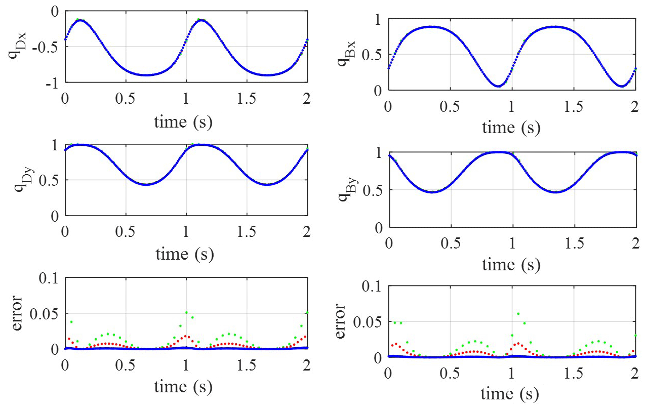
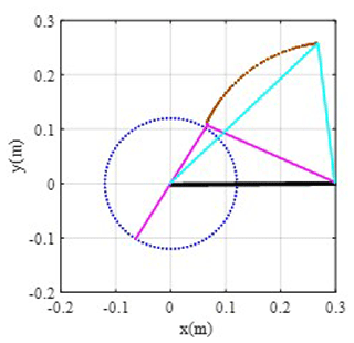
In the kinematics relation, the closed-loop pose–attitude relation is a nonlinear equation. Supposing that the initial rotation angle of the crank is 0 rad, give the initial attitudes of linkage and rocker arbitrarily, and the nonlinear equation is solved using Newton iteration. Supposing that the time steps are h=0.01 s, h=0.03 s and h=0.05 s, the simulation results are expressed by blue, red and green points in Fig. 3 respectively. The rotation speed of the crank is 2π rad s⁻¹. For q_B and q_D, which are direction vectors, their modulus is 1, so the error can be defined as error $=∥\mathit{q}∥-\mathrm{1}$, and the simulation results of the link and rocker's attitudes and the computation errors are as in Fig. 3; the track of the whole system is as in Fig. 4.

Figure 7 Variation in angular momentum and attitudes of the parallelogram mechanism.

Figure 8 The track of the parallelogram mechanism.

From Fig. 3, the simulation results indicate that the attitudes vary in the link and rocker continuously and periodically, and the range of variation is from −1 to 1, which verifies the correctness of the model. Under three different time steps, the simulation results of q coincide, although the errors of q_D and q_B under different time steps have obvious distinctions. From the error variation in Fig. 3, the errors obviously jump under the time step of 0.05s. It means that the bigger time step will lead to a bigger error, although it has a small influence on the attitude results. The biggest errors are generated at 0 rad of the crank, which means that the kinematic equation is difficult to converge at this attitude. As in Fig. 4, the track of the whole system accords with the regular one for a crank and rocker mechanism; the crank makes the whole circle rotation and the rocker swings with a fixed angle.

7.2 Dynamics solution

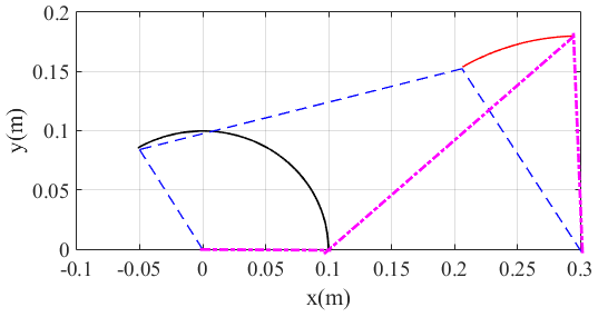
Supposing that the initial angular momentum of the crank is 0 and the initial attitudes of the crank, link and rocker are q₀= [1;0;0.3044;0.9534;-0.3996;0.9167], the simulation time is 5 s, and the dynamics model is solved using ode45 in MATLAB, which is a commonly used Runge–Kutta method. The variation in parameters is as in Fig. 5. According to Fig. 5, the parameters appear to have periodic variation under the action of gravity; the attitudes of the crank, link and rocker also appear to have a periodic character. The maximum value of the attitudes is 1, which verifies the correctness of the results. Figure 6 is the track of the crank–rocker mechanism under free conditions. The simulation results indicate that the closed-loop constraints of the system are conserved in the dynamics simulation.

7.3 Dynamics simulation of parallelogram mechanism

The parallelogram mechanism is a special four-bar mechanism for which the length of the rods on opposite sides is equal. The motion character of the mechanism is that the rods, which are connected to the rack have the same motion, and the link always stays parallel to the rack. For the two sides links can make the whole cycle motion; it also can be seen as a special double-crank mechanism. In the actual computation, the calculation error may lead to tiny variation in the structure of the system, like the length of the rod. The parallelogram mechanism may change to be the crank and rocker mechanism. So the simulation result of the parallelogram mechanism will incur some errors that will create an obvious distinction between the motion of the two side links, and the motion of the link will not be parallel to the rack.

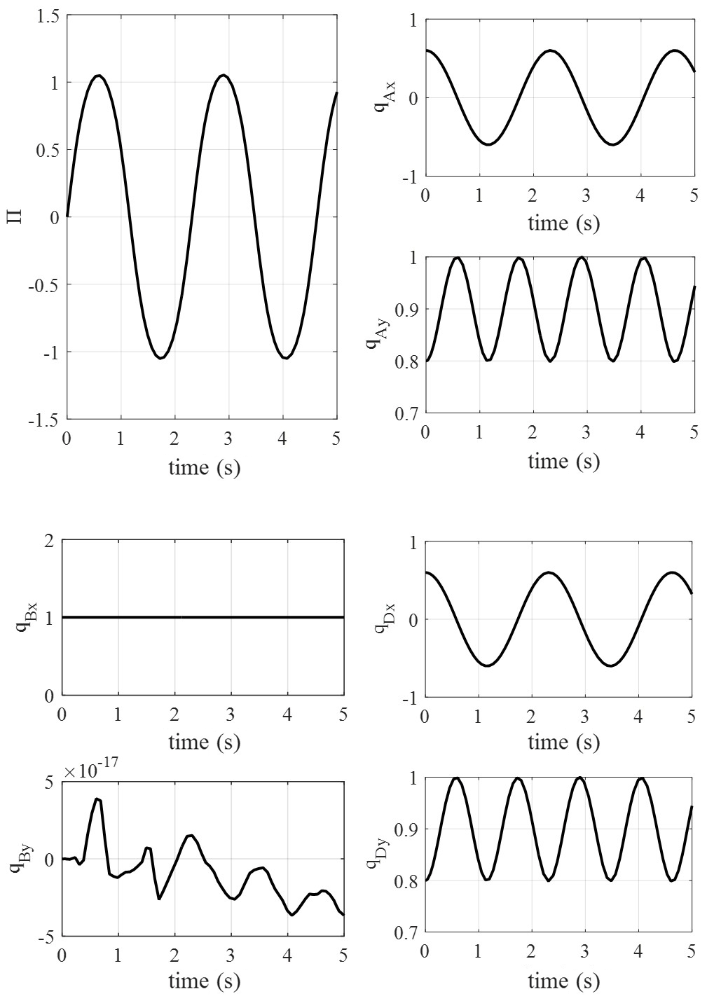
In order to testify the geometry conservation character of the dynamics model, the simulation for the parallelogram mechanism is performed as follows. Supposing that the length of rods is $l_{\mathrm{1}}=l_{\mathrm{3}}=$0.1 m and $l_{\mathrm{2}}=l_{\mathrm{4}}=$0.25 m, the mass and moment inertia are the same with the former simulation. The initial attitude of the system is q₀= [0.6;0.8;1;0;0.6;0.8], the initial momentum is 0, and simulation results are as in Fig. 7.

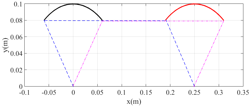
According to Fig. 7, the momentum varies the cyclical movement, which is similar to the single pendulum. It means that the parallelogram mechanism has a similar dynamics character to the single pendulum. The attitudes of the two side links have the same regular motion, which satisfies the motion character of a parallelogram mechanism. The attitude of the link stays parallel to the rack in the whole motion process, which also satisfies the character of a parallelogram mechanism. According to Fig. 8, the track of the system follows the regular parallelogram mechanism; the opposite pair of bars stays parallel during the whole simulation process.

From the above analysis, the derived dynamics model of the four-bar mechanism in this paper can conserve the geometry structure of the system during computation. The lengths of the rods are maintained, which avoids erroneous results.

8 Conclusions

In this research, the dynamics model of the four-bar mechanism is built using the symbol derivation of the differential geometry method. The Lagrange and Hamilton geometry dynamics models are all built, and the numerical computation method is explored. The conclusions are as follows.

1. In the many geometry expression methods, the attitude vector expression for the rod can decrease the difficulty of derivation and expression of the dynamics model.

2. Under the attitude vector expression, the dynamics model can be derived by variation theory, which can package the closed-loop pose–attitude constraint in the dynamics model, so the constraint does not need to be considered.

3. Using the geometry modelling method to build the dynamics model of a four-bar mechanism can avoid the repetitive operation of the closed-loop constraint. All the calculations, which include the variation and derivation, are all aimed at the closed-loop constraint. Also, the results of variation and derivation have a similar structures.

4. With the Legendre transformation, the dynamics model is changed to be the Hamilton type, which uses momentum as a parameter. The model is simplified. The model is reduced by the closed-loop constraint before computation, which makes the programming process simpler.

In this research, a geometry dynamics model for a four-bar mechanism in the plane is built. Based on Lie group theory, the variation in the closed-loop vector space is continuous, which means that this method has a good adaption to the mechanism in space. This work offers a concrete reference for the geometry dynamics modelling of a parallel mechanism in space. The high modularization of the dynamics model without a special numerical algorithm is convenient for software programming, which has a spread prospect in online dynamics simulations and multi-body dynamics for a digital twin in the future.