Modified control variates method based on second-order saddle-point approximation for practical reliability analysis

A novel method is presented for efficiently analyzing the reliability of engineering components and systems with highly nonlinear complex limit state functions. The proposed method begins by transforming the integral of the limit state function into an integral of a highly correlated limit state function using the control variates method. The second-order reliability method is then employed within the control variates framework to approximate the highly correlated limit state function as a quadratic polynomial. Subsequently, the probability of failure is obtained through the estimation of the saddle-point approximation and a small number of samples generated by Latin hypercube sampling. To demonstrate the effectiveness of the proposed method, four examples involving mathematical functions and mechanical problems are solved. The results are compared with those obtained using the second-order reliability method (SORM), control variates based on Monte Carlo simulation (CVMCS) with second-order saddle-point approximation (SOSPA), importance sampling (IS) and Monte Carlo simulation (MCS). The findings demonstrate that, while maintaining high-precision reliability results, the proposed method significantly reduces the number of evaluations of the limit state function through a small number of initial samples. The method is capable of efficiently and accurately solving complex practical engineering reliability problems.

1 Introduction

Safety evaluation of engineering components and systems is crucial for ensuring the economic and efficient operation of industrial equipment. Uncertainties in geometric and material properties of engineering structures arise due to environmental factors and operational influences. In light of these uncertainties, reliability analysis provides a valuable approach to quantifying the ability to fulfill specified system functions within specified conditions and time (Helton et al., 2006; Zhang et al., 2015; Zhao et al., 2017). The probability of failure (PF), based on the limit state function (LSF), is typically expressed as a multidimensional integral of the joint probability density function (PDF) over the random variables. However, directly calculating this multidimensional integral for engineering reliability is challenging. Consequently, various methods for reliability analysis have been developed in recent years. These methods can be broadly categorized into three categories: approximate analytical methods (Hasofer and Lind, 1974; Zhao and Ono, 1999; Meng et al., 2018a), simulation methods (Du, 2008a; Zhang et al., 2018; Meng et al., 2018b) and surrogate model methods (Zhang et al., 2017; Echard et al., 2011; Dai et al., 2015).

In practical engineering problems, the presence of a relatively large number of random variables can result in low computational efficiency for certain methods, such as Monte Carlo simulation (MCS). Therefore, it is preferable to use methods that can provide sufficiently accurate results with a minimum number of evaluations of the limit state function (Lemaire, 2013). In this regard, the approximate analytical methods, such as the first-order reliability method (FORM) and the second-order reliability method (SORM), are advantageous as they can approximate the limit state function with relatively low computational costs. The FORM is widely recognized as one of the most mainstream approximate analytical reliability methods. In recent years, significant improvements have been developed, as evidenced by studies conducted by Chiralaksanakul and Mahadevan (2005), Shayanfar et al. (2017) and Keshtegar and Chakraborty (2018). However, in highly nonlinear complex problems, SORM offers a more accurate approximation of the LSF by using a quadratic polynomial surface. Recent studies have focused on improving SORM, with notable contributions from researchers such as Breitung (1984), Tvedt (1990), Der Kiureghian et al. (1987) and Zhang and Du (2010). Although they have advantages in terms of computation, their accuracy decreases when dealing with reliability problems that involve non-normal random variables and nonlinear limit state functions. Therefore, applying these methods may not be reasonable in such cases. To improve accuracy, some methods based on FORM and SORM have been developed.

Among these methods, saddle-point approximation (SPA) stands out with its advantages of simple calculation, operational feasibility and estimation of the PF without the need to approximate the LSF. Due to the efficiency and accuracy of SPA, scholars have further explored its application in reliability engineering (Xiao et al., 2012; Du, 2008b; Guo, 2014) and integrated it into approximate analytical methods (Du and Sudjianto, 2004; Huang and Du, 2008; Huang et al., 2018). Du and Sudjianto (2004) proposed the first-order saddle-point approximation (FOSA) method, which involves expanding the cumulant-generating function of the LSF using a first-order Taylor series expansion around the most probable point (MPP) and estimating the PF using saddle-point approximation. Huang and Du (2008) introduced the modified variance function-based saddle-point approximation method (MVFOSA), which transforms highly nonlinear LSFs into approximate linear functions at the mean point of each random variable, resulting in a more efficient approach. Huang et al. (2018) developed a new second-order reliability method based on saddle-point approximation, which obtains a second-order approximation of the LSF by performing a second-order Taylor series expansion around the MPP. However, it is important to acknowledge the existence of approximation errors and the potential accuracy disparity between approximate analytical methods and MCS in engineering applications.

Since approximate analytical methods do not introduce any errors into probability estimation, they cannot quantify the inherent approximation errors of these methods. Therefore, there exists a difference in accuracy between approximate analytical methods and simulation methods. MCS (Metropolis and Ulam, 1949; Zio, 2013) and its variants, such as importance sampling (IS) (Papaioannou et al., 2019) and subset simulation (SS) (Au and Beck, 2001), are more robust for complex limit state functions. MCS is most accurate as a standard for testing other theoretical methods. Despite these advantages, in order to achieve an acceptable level of accuracy, the number of random samples required by MCS grows exponentially for practical engineering problems with small failure probabilities. If the failure probability is on the order of 10^−k, MCS requires 10^k+2–10^k+3 samples to achieve the corresponding accuracy (Binder, 1987). Because the variance of MCS estimates is inversely proportional to the failure probability, some studies (Melchers, 1989; Au and Beck, 2001; Rubinstein and Kroese, 2016; Oates et al., 2016) have explored the use of variance reduction techniques in simulation methods to reduce the variance of MCS.

Among these variance reduction techniques, the control variable (CV) method (Law et al., 2000) stands out for its relatively simple operation and broad applicability, as it has almost no restrictions on its range of application. The CV method has been employed recently in reliability analysis. For instance, Kawai (2020) utilized both importance sampling and control variates to construct and investigate an adaptive variance reduction framework. Portier and Segers (2019) successfully reduced the variance of Monte Carlo integration using control variates in a multiple linear regression model. Dimarco and Pareschi (2020) introduced a multiscale control variates strategy to enhance the efficiency of numerical calculations for kinetic equations with stochastic parameters, particularly in high-dimensional problems. Additionally, in engineering practice, where reliability problems often involve high dimensionality and small failure probabilities, the CV method is frequently combined with other techniques. Rashki (2018) introduced a new formulation for approximating small failure probabilities, leveraging the adaptive cooperation of SS and the CV method. To minimize the number of evaluations of the LSF, Ameryan et al. (2022) proposed a novel approach that integrates an active learning kriging metamodel (AK-MCS) and the sequential space conversion method (SESC), where the SESC formulation is derived using the control variates method. Moreover, to enhance the efficiency of addressing high-dimensional problems, Mehni and Mehni (2023) presented a method for improving the performance of cross-entropy-based Gaussian mixture importance sampling, incorporating a control variates scheme to further enhance its effectiveness.

In this study, the control variates method is combined with variance reduction sampling techniques to enhance the efficiency of probability estimation. These techniques, with significantly smaller sample sizes compared to MCS-based CVs, often result in a substantial reduction in the number of evaluations of the LSF. Among these techniques, Latin hypercube sampling (LHS), initially proposed by Mckay et al. (1979), is a widely used multidimensional stratified sampling method in engineering practice. Zou et al. (2008) employed an optimal symmetric LHS technique to construct the response surface of the indicator function for multiple limit state and multiple design point problems. Yang et al. (2005) utilized the optimal LHS method to uniformly distribute sampling points across the entire design space, thereby improving the accuracy of a real-world frontal impact metamodel. Christensen et al. (2017) employed a novel constrained nested orthogonal-maximin Latin hypercube approach for sampling to determine variable-shape mold configurations used in the training and test sets. LHS exhibits characteristics such as quick convergence and uniformly distributed samples. Therefore, using LHS to generate samples for the control variates method can significantly improve computational efficiency.

To address the reliability issues of engineering components and systems characterized by high nonlinearity and complexity with limited samples, this study proposes a method that combines second-order saddle-point approximation (SOSPA) with control variable Latin hypercube sampling (CVLHS). The proposed method leverages the benefits of both variance reduction techniques and approximate analytical methods. By doing so, it achieves high-precision reliability results while significantly reducing the number of evaluations of the limit state function. The remainder of the paper is organized as follows. Section 2 discusses the method combining CVLHS and SOSPA. Section 3 outlines the implementation procedure of the proposed method in real-world applications. Section 4 presents two numerical examples and two engineering cases to demonstrate the efficiency and accuracy of the proposed method. Finally, Sect. 5 provides conclusions.

2 CVLHS with SOSPA

To increase the efficiency of the MCS, based on the theory of the CV method, the index function of the highly correlated limit state function (LSF) as the CV is used to convert the original index function in the PF multidimensional integral. By incorporating LHS into the CV method, only a small number of samples need to be generated to remove the errors raised from the highly correlated LSF. Combining the expectation of the CV estimated by SOSPA, PF is estimated accurately without any simplification and assumptions.

2.1 CV for the failure probability function

The PF is expressed as the integral of the joint PDF f_X(x) over the n-dimensional random variable vector $\mathit{x}=\left[x_{\mathrm{1}},x_{\mathrm{2}},\mathrm{\dots },x_n\right]$:

$$\begin{array}{}\text{(1)}& P_f=\underset{F}{\int }{f}_X\left(\mathit{x}\right)\mathrm{d}\mathit{x}={\int }_X{I}_F\left(\mathit{x}\right)f_X\left(\mathit{x}\right)\mathrm{d}x,\end{array}$$

where F is the failure domain, $F=\left\{\mathit{x}:g\left(\mathit{x}\right)\le \mathrm{0}\right\}$, g(x) is the LSF and I_F is the index function:

$$\begin{array}{}\text{(2)}& I_F\left(\mathit{x}\right)=\left\{\begin{array}{ll}\mathrm{1},& \mathit{x}\in F,\\ \mathrm{0},& \mathit{x}\notin F.\end{array}\right.\end{array}$$

This integral can be described as an expectation of I_F(x), and with the N randomly sampled variable vector x, it is approximated as follows:

$$\begin{array}{}\text{(3)}& P_f={\int }_X{I}_F\left(\mathit{x}\right)f_X\left(\mathit{x}\right)\mathrm{d}\mathit{x}=E\left[I_F\left(\mathit{x}\right)\right]\approx {\displaystyle \frac{\mathrm{1}}{N}}\sum _{i=\mathrm{1}}^N{I}_F\left({\mathit{x}}_i\right).\end{array}$$

If g_c(x) is the highly correlated LSF of g(x), the corresponding failure domain can be denoted as $F_{\mathrm{c}}=\left\{\mathit{x}:g_{\mathrm{c}}\left(\mathit{x}\right)\le \mathrm{0}\right\}$. Moreover, $I_{F_{\mathrm{c}}}$ is the index function as a CV which is the high correlation of I_F, and similarly to Eq. (2), $I_{F_{\mathrm{c}}}\left(\mathit{x}\right)=\left\{\begin{array}{ll}\mathrm{1},& \mathit{x}\in F_{\mathrm{c}}\\ \mathrm{0},& \mathit{x}\notin F_{\mathrm{c}}\end{array}\right.$. According to the CV-reduction technique (Rubinstein and Kroese, 2016), the new index function is defined by

$$\begin{array}{}\text{(4)}& I_{F_{\mathrm{CV}}}\left(\mathit{x}\right)=I_F\left(\mathit{x}\right)-\mathit{\rho }\left[I_{F_{\mathrm{c}}}\left(\mathit{x}\right)-E\left[I_{F_{\mathrm{c}}}\left(\mathit{x}\right)\right]\right],\end{array}$$

where ρ is the correction coefficient.

Therefore, by substituting Eq. (4) into Eq. (2), the failure probability integral by CV is rewritten as

$$\begin{array}{}\text{(5)}& \begin{array}{rl}{P}_{f_{\mathrm{CV}}}& ={\int }_X{I}_{F_{\mathrm{CV}}}\left(\mathit{x}\right)f_X\left(\mathit{x}\right)\mathrm{d}x={\int }_X{I}_F\left(\mathit{x}\right)f_X\left(\mathit{x}\right)\mathrm{d}x\\ & -\mathit{\rho }{\int }_X{I}_{F_{\mathrm{c}}}\left(\mathit{x}\right)f_X\left(\mathit{x}\right)\mathrm{d}x+\mathit{\rho }E\left[I_{F_{\mathrm{c}}}\left(\mathit{x}\right)\right]\\ & \approx \mathit{\rho }\cdot P_{f_{\mathrm{c}}}+{\displaystyle \frac{\mathrm{1}}{N}}\sum _{i=\mathrm{1}}^N\left(I_F\left({\mathit{x}}_i\right)-\mathit{\rho }\cdot I_{F_{\mathrm{c}}}\left({\mathit{x}}_i\right)\right),\end{array}\end{array}$$

where $P_{f_{\mathrm{c}}}$ is the PF of the highly correlated LSF g_c(x). To simplify the failure probability function, the posterior portion of Eq. (5) will be zero, i.e., $\frac{\mathrm{1}}{N}\sum _{i=\mathrm{1}}^N\left(I_F\left({\mathit{x}}_i\right)-\mathit{\rho }\cdot I_{F_{\mathrm{c}}}\left({\mathit{x}}_i\right)\right)=\mathrm{0}$. In the light of Eq. (3), the correction coefficient ρ is estimated by the ratio of the expectation of the index functions:

$$\begin{array}{}\text{(6)}& \mathit{\rho }=\sum _{i=\mathrm{1}}^N{I}_F\left({\mathit{x}}_i\right)/\sum _{i=\mathrm{1}}^N{I}_{F_{\mathrm{c}}}\left({\mathit{x}}_i\right).\end{array}$$

Then, Eq. (5) can be simplified to

$$\begin{array}{}\text{(7)}& P_{f_{\mathrm{CV}}}=\mathit{\rho }\cdot P_{f_{\mathrm{c}}}.\end{array}$$

2.2 Quadratic polynomial surface approximation of the LSF

In this study, to ensure the accuracy of reliability analysis for the high-nonlinearity reliability problems, the quadratic polynomial is selected as the highly correlated LSF g_c(x). By calculating the second derivative, the quadratic polynomial approximation of g(x) can consider the concave direction and curvature of the limit state surface near the MPP. The highly correlated LSF is expanded into a quadratic term of Taylor series at the MPP x^∗ as follows:

$$\begin{array}{}\text{(8)}& \begin{array}{rl}{g}_{\mathrm{c}}\left(\mathit{x}\right)& =g\left({\mathit{x}}^{\ast }\right)+\mathrm{\nabla }g\left({\mathit{x}}^{\ast }{)}^{\mathrm{T}}\right(\mathit{x}-{\mathit{x}}^{\ast })\\ & +{\displaystyle \frac{\mathrm{1}}{\mathrm{2}}}(\mathit{x}-{\mathit{x}}^{\ast }{)}^{\mathrm{T}}{\mathrm{\nabla }}^{\mathrm{2}}g({\mathit{x}}^{\ast }\left)\right(\mathit{x}-{\mathit{x}}^{\ast }),\end{array}\end{array}$$

where ∇g(x^∗) is the vector of partial derivatives at the MPP; ∇²g(x^∗) is the Hessian matrix of g(x) at the MPP; and x^∗ is the MPP, which is solved by iterative optimization using the mean of x as the initial search point:

$$\begin{array}{}\text{(9)}& \left\{\begin{array}{l}min\mathrm{|}\mathrm{|}\mathit{x}\mathrm{|}\mathrm{|},\\ \text{subject}\text{to}g\left(\mathit{x}\right)=\mathrm{0}.\end{array}\right.\end{array}$$

where ||x|| is the distance from the origin to the x on the limit state surface.

2.3 Latin hypercube sampling

The correction coefficient ρ in Eq. (6) is obtained based on MCS generally. Nevertheless, for complicated high-dimensional problems, MCS requires huge amounts of computation for accurate estimation. To further reduce the computational cost, LHS is employed to generate the initial samples based on the original LSF g(x) and the highly correlated LSF g_c(x) denoted by the Taylor expanded quadratic polynomial, respectively.

To sample N initial points of x, the independent U(0,l) (uniformly distributed on [0,1]) random variables are represented as U(i,j) ($i=\mathrm{1},\mathrm{\dots },N,j=\mathrm{1},\mathrm{\dots },n)$. The corresponding scaling probability for each random number U(i,j) can be given by

$$\begin{array}{}\text{(10)}& P(i,j)={\displaystyle \frac{U(i,j)+(j-\mathrm{1})}{N}}\left(i=\mathrm{1},\mathrm{\dots },n,j=\mathrm{1},\mathrm{\dots },N\right).\end{array}$$

Then the corresponding components $x_{i,j}(i=\mathrm{1},\mathrm{\dots },N,j=\mathrm{1},\mathrm{\dots },n)$ can be generated by inverse distribution functions. LHS considers the total sampling range of random variables with a small number of samples. Under the premise of ensuring accuracy, the efficiency of the sampling is improved. The initial correction coefficient ρ₀ is obtained by the N initial samples x, and the result of ρ is optimized by N_add by adding samples until more than 20 failure points are reached. The process of LHS is shown in Fig. 1.

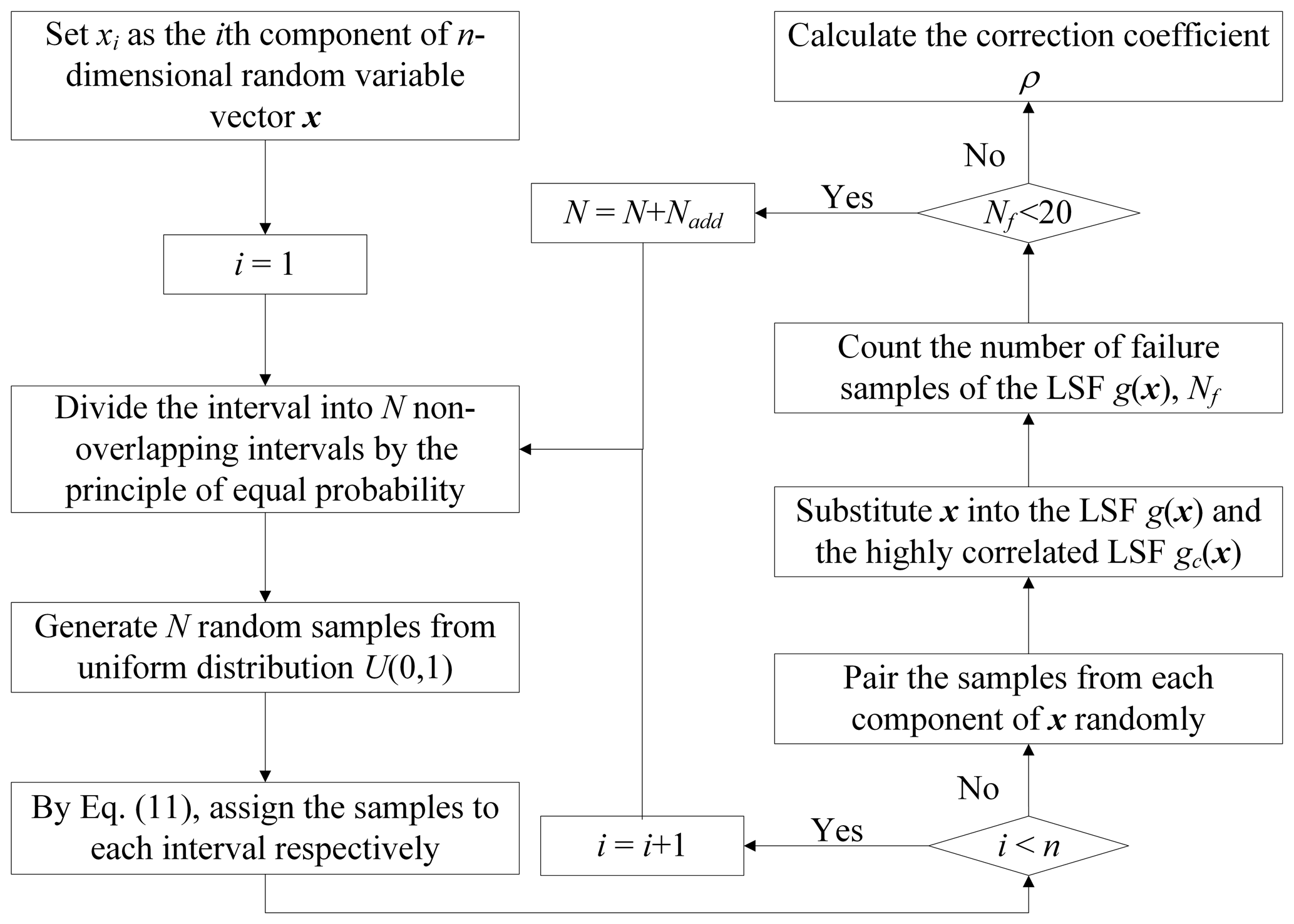
Figure 1 The procedure to generate the initial samples and optimize the correction coefficient by LHS.

2.4 SOSPA for the PF of the highly correlated LSF

For the computational advantage of SPA on a quadratic polynomial, SOSPA is more accurate than the other common SORM (Huang et al., 2018). Therefore, it is utilized to approximate the PF of the highly correlated LSF in this study. It employs an inverse Fourier transform to obtain the cumulative distribution function (CDF) of an exponential power series expression based on a saddle point by the moment-generating function (MGF) and the cumulant-generating function (CGF).

The MGF (Broda and Paolella, 2011) of the highly correlated LSF g_c(x), where $\mathit{x}\sim N(\mathit{\mu },\mathit{\sigma })$, is given by

$$\begin{array}{}\text{(11)}& \begin{array}{rl}& M_{g_{\mathrm{c}}}\left(t\right)=E\left[e^{t{g}_{\mathrm{c}}}\right]={\int }_{-\mathrm{\infty }}^{\mathrm{\infty }}{e}^{t{g}_{\mathrm{c}}}{f}_X\left(\mathit{x}\right)\mathrm{d}\mathit{x}\\ & =\exp \left\{t\left(a+{\mathit{b}}^{\mathrm{T}}\mathit{\mu }+{\mathit{\mu }}^{\mathrm{T}}\mathit{c}\mathit{\mu }\right)+{\displaystyle \frac{t^{\mathrm{2}}}{\mathrm{2}}}\sum _{i=\mathrm{1}}^n{\displaystyle \frac{d_i^{\mathrm{2}}}{\mathrm{1}-\mathrm{2}t{\mathit{\lambda }}_i}}\right\}\\ & \prod _{i=\mathrm{1}}^n{\left(\mathrm{1}-\mathrm{2}t{\mathit{\lambda }}_i\right)}^{-\mathrm{0.5}},\end{array}\end{array}$$

where ${\mathit{\lambda }}_{\mathrm{1}},\mathrm{\dots },{\mathit{\lambda }}_n$ and P are the eigenvalues and eigenvectors of c and $\mathit{P}\mathit{c}{\mathit{P}}^{\mathrm{T}}=\text{diag}({\mathit{\lambda }}_{\mathrm{1}},\mathrm{\dots },{\mathit{\lambda }}_n)$ with P orthogonal, $\mathit{d}={\left[d_{\mathrm{1}},d_{\mathrm{2}},\mathrm{\dots },d_n\right]}^{\mathrm{T}}={\mathit{P}}^{\mathrm{T}}\left({\mathit{\sigma }}^{\mathrm{0.5}}\mathit{b}+\mathrm{2}{\mathit{\sigma }}^{\mathrm{0.5}}\mathit{c}\mathit{\mu }\right)$, $a=\mathrm{0.5}{\mathit{x}}^{\ast T}{\mathrm{\nabla }}^{\mathrm{2}}{g}_{\mathrm{c}}\left({\mathit{x}}^{\ast }\right){\mathit{x}}^{\ast }-\mathrm{\nabla }{g}_{\mathrm{c}}({\mathit{x}}^{\ast }{)}^{\mathrm{T}}{\mathit{x}}^{\ast }$, $\mathit{b}=\mathrm{\nabla }{g}_{\mathrm{c}}\left({\mathit{x}}^{\ast }\right)-{\mathrm{\nabla }}^{\mathrm{2}}{g}_{\mathrm{c}}\left({\mathit{x}}^{\ast }\right){\mathit{x}}^{\ast }$ and $\mathit{c}=\mathrm{0.5}{\mathrm{\nabla }}^{\mathrm{2}}{g}_{\mathrm{c}}\left({\mathit{x}}^{\ast }\right)$.

Moreover, the CGF of g_c is given by

$$\begin{array}{}\text{(12)}& \begin{array}{rl}{K}_{g_{\mathrm{c}}}\left(t\right)& =\ln \left(M_{g_{\mathrm{c}}}\left(t\right)\right)=t\left(a+{\mathit{b}}^{\mathrm{T}}\mathit{\mu }+{\mathit{\mu }}^{\mathrm{T}}\mathit{c}\mathit{\mu }\right)\\ & +{\displaystyle \frac{t^{\mathrm{2}}}{\mathrm{2}}}\sum _{i=\mathrm{1}}^n{d}_i^{\mathrm{2}}{\mathit{\vartheta }}_i+{\displaystyle \frac{\mathrm{1}}{\mathrm{2}}}\sum _{i=\mathrm{1}}^n\ln {\mathit{\vartheta }}_i,\end{array}\end{array}$$

where ${\mathit{\vartheta }}_i=(\mathrm{1}-\mathrm{2}t{\mathit{\lambda }}_i{)}^{-\mathrm{1}}$.

Then the derivatives of $K_{g_{\mathrm{c}}}\left(t\right)$ can be determined as follows.

$$\begin{array}{}\text{(13)}& \begin{array}{rl}{K}_{g_{\mathrm{c}}}^{\left(\mathrm{1}\right)}\left(t\right)& =a+{\mathit{b}}^{\mathrm{T}}\mathit{\mu }+{\mathit{\mu }}^{\mathrm{T}}\mathit{c}\mathit{\mu }\\ & +\sum _{i=\mathrm{1}}^n\left(t{d}_i^{\mathrm{2}}{\mathit{\vartheta }}_i+t^{\mathrm{2}}{d}_i^{\mathrm{2}}{\mathit{\vartheta }}_i^{\mathrm{2}}{\mathit{\lambda }}_i+{\mathit{\vartheta }}_i{\mathit{\lambda }}_i\right)\end{array}\end{array}$$

$$\begin{array}{}\text{(14)}& K_{g_{\mathrm{c}}}^{\left(\mathrm{2}\right)}\left(t\right)=\sum _{i=\mathrm{1}}^n\left(d_i^{\mathrm{2}}{\mathit{\vartheta }}_i+\mathrm{4}t{d}_i^{\mathrm{2}}{\mathit{\vartheta }}_i^{\mathrm{2}}{\mathit{\lambda }}_i+\mathrm{4}{t}^{\mathrm{2}}{d}_i^{\mathrm{2}}{\mathit{\vartheta }}_i^{\mathrm{3}}{\mathit{\lambda }}_i^{\mathrm{2}}+\mathrm{2}{\mathit{\vartheta }}_i^{\mathrm{2}}{\mathit{\lambda }}_i^{\mathrm{2}}\right)\end{array}$$

$$\begin{array}{}\text{(15)}& \begin{array}{rl}& K_{g_{\mathrm{c}}}^{\left(\mathrm{3}\right)}\left(t\right)\\ & =\sum _{i=\mathrm{1}}^n(\mathrm{6}{d}_i^{\mathrm{2}}{\mathit{\vartheta }}_i^{\mathrm{2}}{\mathit{\lambda }}_i+\mathrm{24}t{d}_i^{\mathrm{2}}{\mathit{\vartheta }}_i^{\mathrm{3}}{\mathit{\lambda }}_i^{\mathrm{2}}+\mathrm{24}{t}^{\mathrm{2}}{d}_i^{\mathrm{2}}{\mathit{\vartheta }}_i^{\mathrm{4}}{\mathit{\lambda }}_i^{\mathrm{3}}+\mathrm{8}{\mathit{\vartheta }}_i^{\mathrm{3}}{\mathit{\lambda }}_i^{\mathrm{3}})\end{array}\end{array}$$

$$\begin{array}{}\text{(16)}& \begin{array}{rl}{K}_{g_{\mathrm{c}}}^{\left(\mathrm{4}\right)}\left(t\right)=\sum _{i=\mathrm{1}}^n(& \mathrm{48}{d}_i^{\mathrm{2}}{\mathit{\vartheta }}_i^{\mathrm{3}}{\mathit{\lambda }}_i^{\mathrm{2}}+\mathrm{192}t{d}_i^{\mathrm{2}}{\mathit{\vartheta }}_i^{\mathrm{4}}{\mathit{\lambda }}_i^{\mathrm{3}}\\ & +\mathrm{192}{t}^{\mathrm{2}}{d}_i^{\mathrm{2}}{\mathit{\vartheta }}_i^{\mathrm{5}}{\mathit{\lambda }}_i^{\mathrm{4}}+\mathrm{48}{\mathit{\vartheta }}_i^{\mathrm{4}}{\mathit{\lambda }}_i^{\mathrm{4}})\end{array}\end{array}$$

By numerically integrating the PDF of SPA (Lugannani and Rice, 1980), the CDF of g_c can be approximated as

$$\begin{array}{}\text{(17)}& F_{g_{\mathrm{c}}}\left(g_{\mathrm{c}\mathrm{0}}\right)=P\left\{g_{\mathrm{c}}\le g_{\mathrm{c}\mathrm{0}}\right\}\approx \mathrm{\Phi }\left(w\right)+\mathit{\varphi }\left(w\right)\left({\displaystyle \frac{\mathrm{1}}{w}}-{\displaystyle \frac{\mathrm{1}}{v}}\right),\end{array}$$

where Φ(⋅) and φ(⋅) are the CDF and PDF of the standard normal distribution, respectively, and w and v are parameters expressed as

$$\begin{array}{}\text{(18)}& w=\text{sgn}\left(t_{\mathrm{s}}\right){\left\{\mathrm{2}\left[t_{\mathrm{s}}{g}_{\mathrm{c}\mathrm{0}}-K_{g_{\mathrm{c}}}\left(t_{\mathrm{s}}\right)\right]\right\}}^{\mathrm{0.5}},\end{array}$$

$$\begin{array}{}\text{(19)}& v=t_{\mathrm{s}}{\left[K_{g_{\mathrm{c}}}^{\left(\mathrm{2}\right)}\left(t_{\mathrm{s}}\right)\right]}^{\mathrm{0.5}},\end{array}$$

where t_s is the saddle point, $K_{g_{\mathrm{c}}}^{\left(\mathrm{2}\right)}(\cdot )$ are the second-order derivatives of $K_{g_{\mathrm{c}}}(\cdot )$, and sgn(t_s) is a symbolic function and can be +1, −1 or 0, corresponding to t_s>0, t_s<0 and t_s=0.

Furthermore, the second-order CDF of g_c is

$$\begin{array}{}\text{(20)}& \begin{array}{rl}{\stackrel{\mathrm{̃}}{F}}_{g_{\mathrm{c}}}\left(g_{\mathrm{c}\mathrm{0}}\right)& =P\left\{g_{\mathrm{c}}\le g_{\mathrm{c}\mathrm{0}}\right\}\\ & \approx F_{g_{\mathrm{c}}}\left(g_{\mathrm{c}\mathrm{0}}\right)-\mathit{\varphi }\left(w\right)\\ & \left(v^{-\mathrm{1}}\left({\displaystyle \frac{{\mathit{\kappa }}_{\mathrm{4}}}{\mathrm{8}}}-{\displaystyle \frac{\mathrm{5}}{\mathrm{24}}}{\mathit{\kappa }}_{\mathrm{3}}^{\mathrm{2}}\right)-v^{-\mathrm{3}}-{\displaystyle \frac{{\mathit{\kappa }}_{\mathrm{3}}}{\mathrm{2}{u}^{\mathrm{2}}}}+w^{-\mathrm{3}}\right),\end{array}\end{array}$$

where ${\mathit{\kappa }}_i=K_{g_{\mathrm{c}}}^{\left(i\right)}\left(t_{\mathrm{s}}\right)/{\left[K_{g_{\mathrm{c}}}^{\left(\mathrm{2}\right)}\left(t_{\mathrm{s}}\right)\right]}^{\mathrm{0.5}i}$.

Then, making g_c0=0, the PF $P_{f_{\mathrm{c}}}$ can be easily calculated from the second-order CDF ${\stackrel{\mathrm{̃}}{F}}_{g_{\mathrm{c}}}\left(\mathrm{0}\right)$ corresponding to the strongly correlated LSF g_c(x)≤0, i.e.,

$$\begin{array}{}\text{(21)}& P_{f_{\mathrm{c}}}={\stackrel{\mathrm{̃}}{F}}_{g_{\mathrm{c}}}\left(\mathrm{0}\right).\end{array}$$

3 Implementation procedure

To ensure the accuracy of the PF, the coefficient of variation of the PF is calculated as the stop condition for loop operation. The new sample vector x_new is sequentially added to the sample set until the coefficient of variation of the PF has to be convergent.

3.1 The estimator statistical property

The expectation of PF in Eq. (7) is estimated as

$$\begin{array}{}\text{(22)}& E\left(P_{f_{\mathrm{CV}}}\right)=E\left(\mathit{\rho }\cdot P_{f_{\mathrm{c}}}\right)=\mathit{\rho }\cdot E\left({\stackrel{\mathrm{̃}}{F}}_{g_{\mathrm{c}}}\left(\mathrm{0}\right)\right).\end{array}$$

Since the estimation PF by LHS is the unbiased estimation (McKay et al., 1979), the expectations of the PF of the original LSF and the highly correlated LSF are

$$\begin{array}{}\text{(23)}& E\left(P_{f_{\mathrm{LHS}}}\right)=E\left(I_F\left(\mathit{x}\right)\right)\approx {\displaystyle \frac{\mathrm{1}}{N}}\sum _{i=\mathrm{1}}^N{I}_F\left({\mathit{x}}_i\right),\end{array}$$

$$\begin{array}{}\text{(24)}& E\left(P_{f_{c_{\mathrm{LHS}}}}\right)=E\left(I_{F_{\mathrm{c}}}\left(\mathit{x}\right)\right)\approx {\displaystyle \frac{\mathrm{1}}{N}}\sum _{i=\mathrm{1}}^N{I}_{F_{\mathrm{c}}}\left({\mathit{x}}_i\right).\end{array}$$

Therefore, the correction coefficient ρ is estimated by LHS:

$$\begin{array}{}\text{(25)}& \begin{array}{rl}\mathit{\rho }& =E\left(P_{f_{\mathrm{LHS}}}\right)/E\left(P_{f_{c_{\mathrm{LHS}}}}\right)\\ & ={\displaystyle \frac{\mathrm{1}}{N}}\sum _{i=\mathrm{1}}^N{I}_F\left({\mathit{x}}_i\right)/{\displaystyle \frac{\mathrm{1}}{N}}\sum _{i=\mathrm{1}}^N{I}_{F_{\mathrm{c}}}\left({\mathit{x}}_i\right)=P_{f_{\mathrm{LHS}}}/P_{f_{c_{\mathrm{LHS}}}}\end{array}\end{array}$$

The expectation of PF is given by

$$\begin{array}{}\text{(26)}& E\left(P_{f_{\mathrm{CV}}}\right)={\displaystyle \frac{E\left(P_{f_{\mathrm{LHS}}}\right)}{E\left(P_{f_{{\mathrm{c}}_{\mathrm{LHS}}}}\right)}}\cdot E\left({\stackrel{\mathrm{̃}}{F}}_{g_{\mathrm{c}}}\left(\mathrm{0}\right)\right).\end{array}$$

According to the theory of control variate estimator property, the variance of PF by the proposed approach may be estimated as

$$\begin{array}{}\text{(27)}& \begin{array}{rl}\text{Var}\left(P_{f_{\mathrm{CV}}}\right)& =\text{Var}\left(P_{f_{\mathrm{LHS}}}\right)+{\mathit{\rho }}^{\mathrm{2}}\text{Var}\left(P_{f_{c_{\mathrm{LHS}}}}\right)\\ & -\mathrm{2}\mathit{\rho }\text{Cov}\left(P_{f_{\mathrm{LHS}}},P_{f_{c_{\mathrm{LHS}}}}\right)\\ & =\text{Var}\left(P_{f_{\mathrm{LHS}}}\right)+{\displaystyle \frac{E^{\mathrm{2}}\left(P_{f_{\mathrm{LHS}}}\right)}{E^{\mathrm{2}}\left(P_{f_{c_{\mathrm{LHS}}}}\right)}}\cdot \text{Var}\left(P_{f_{c_{\mathrm{LHS}}}}\right)\\ & -\mathrm{2}\cdot {\displaystyle \frac{E\left(P_{f_{\mathrm{LHS}}}\right)}{E\left(P_{f_{c_{\mathrm{LHS}}}}\right)}}\cdot \text{Cov}\left(P_{f_{\mathrm{LHS}}},P_{f_{c_{\mathrm{LHS}}}}\right).\end{array}\end{array}$$

Due to the expectation and the variance of $P_{f_{\mathrm{CV}}}$, the coefficient of variation ${\mathit{\delta }}_{P_{f_{\mathrm{CV}}}}$ can be estimated as

$$\begin{array}{}\text{(28)}& \begin{array}{rl}& {\mathit{\delta }}_{P_{f_{\mathrm{CV}}}}={\displaystyle \frac{\sqrt{\text{Var}\left(P_{f_{\mathrm{CV}}}\right)}}{E\left(P_{f_{\mathrm{CV}}}\right)}}\\ & ={\displaystyle \frac{\sqrt{\text{Var}\left(P_{f_{\mathrm{LHS}}}\right)+\frac{E^{\mathrm{2}}\left(P_{f_{\mathrm{LHS}}}\right)}{E^{\mathrm{2}}\left(P_{f_{c_{\mathrm{LHS}}}}\right)}\cdot \text{Var}\left(P_{f_{c_{\mathrm{LHS}}}}\right)-\mathrm{2}\cdot \frac{E\left(P_{f_{\mathrm{LHS}}}\right)}{E\left(P_{f_{c_{\mathrm{LHS}}}}\right)}\cdot \text{Cov}\left(P_{f_{\mathrm{LHS}}},P_{f_{c_{\mathrm{LHS}}}}\right)}}{\frac{E\left(P_{f_{\mathrm{LHS}}}\right)}{E\left(P_{f_{c_{\mathrm{LHS}}}}\right)}\cdot E\left({\stackrel{\mathrm{̃}}{F}}_{g_{\mathrm{c}}}\left(\mathrm{0}\right)\right)}}\\ & =\sqrt{{\displaystyle \frac{E^{\mathrm{2}}\left(P_{f_{c_{\mathrm{LHS}}}}\right)\cdot \text{Var}\left(P_{f_{\mathrm{LHS}}}\right)}{E^{\mathrm{2}}\left(P_{f_{\mathrm{LHS}}}\right)\cdot {\stackrel{\mathrm{̃}}{F}}_{g_{\mathrm{c}}}^{\mathrm{2}}\left(\mathrm{0}\right)}}+{\displaystyle \frac{\text{Var}\left(P_{f_{c_{\mathrm{LHS}}}}\right)}{{\stackrel{\mathrm{̃}}{F}}_{g_{\mathrm{c}}}^{\mathrm{2}}\left(\mathrm{0}\right)}}-{\displaystyle \frac{\mathrm{2}\cdot E\left(P_{f_{c_{\mathrm{LHS}}}}\right)\cdot \text{Cov}\left(P_{f_{\mathrm{LHS}}},P_{f_{c_{\mathrm{LHS}}}}\right)}{E\left(P_{f_{\mathrm{LHS}}}\right)\cdot {\stackrel{\mathrm{̃}}{F}}_{g_{\mathrm{c}}}^{\mathrm{2}}\left(\mathrm{0}\right)}}}.\end{array}\end{array}$$

Hereinto, the variances of the PF by LHS are expressed as

$$\begin{array}{}\text{(29)}& \begin{array}{ll}\left\{\begin{array}{l}\begin{array}{rl}& \text{Var}\left(P_{f_{\mathrm{LHS}}}\right)\\ & =\text{Var}\left({\displaystyle \frac{\mathrm{1}}{N}}\sum _{i=\mathrm{1}}^N{I}_F\left({\mathit{x}}_i\right)\right)\end{array}\\ \begin{array}{rl}& ={\displaystyle \frac{\mathrm{1}}{N}}\text{Var}\left(I_F\left(\mathit{x}\right)\right)+{\displaystyle \frac{\mathrm{1}}{N}}(N-\mathrm{1})\\ & \text{cov}\left(I_F\left({\mathit{x}}_{\mathrm{1},j}\right),I_F\left({\mathit{x}}_{\mathrm{2},j}\right)\right)\end{array}\end{array}\right.& ,j=\mathrm{1},\mathrm{2},\mathrm{\dots },n.\end{array}\end{array}$$

$$\begin{array}{}\text{(30)}& \begin{array}{ll}\left\{\begin{array}{l}\begin{array}{rl}& \text{Var}\left(P_{f_{c_{\mathrm{LHS}}}}\right)\\ & =\text{Var}\left({\displaystyle \frac{\mathrm{1}}{N}}\sum _{i=\mathrm{1}}^N{I}_{F_{\mathrm{c}}}\left({\mathit{x}}_i\right)\right)\end{array}\\ \begin{array}{rl}& ={\displaystyle \frac{\mathrm{1}}{N}}\text{Var}\left(I_{F_{\mathrm{c}}}\left(\mathit{x}\right)\right)+{\displaystyle \frac{\mathrm{1}}{N}}(N-\mathrm{1})\\ & \text{cov}\left(I_{F_{\mathrm{c}}}\left({\mathit{x}}_{\mathrm{1},j}\right),I_{F_{\mathrm{c}}}\left({\mathit{x}}_{\mathrm{2},j}\right)\right)\end{array}\end{array}\right.& ,j=\mathrm{1},\mathrm{2},\mathrm{\dots },n\end{array}\end{array}$$

Stein (1987) proved that $\frac{\mathrm{1}}{N}(N-\mathrm{1})\text{cov}\left(I_{F_{\mathrm{c}}}\left({\mathit{x}}_{\mathrm{1},j}\right),I_{F_{\mathrm{c}}}\left({\mathit{x}}_{\mathrm{2},j}\right)\right)$ is a non-positive value. Therefore, LHS has a smaller variance than MCS and is easier to converge.

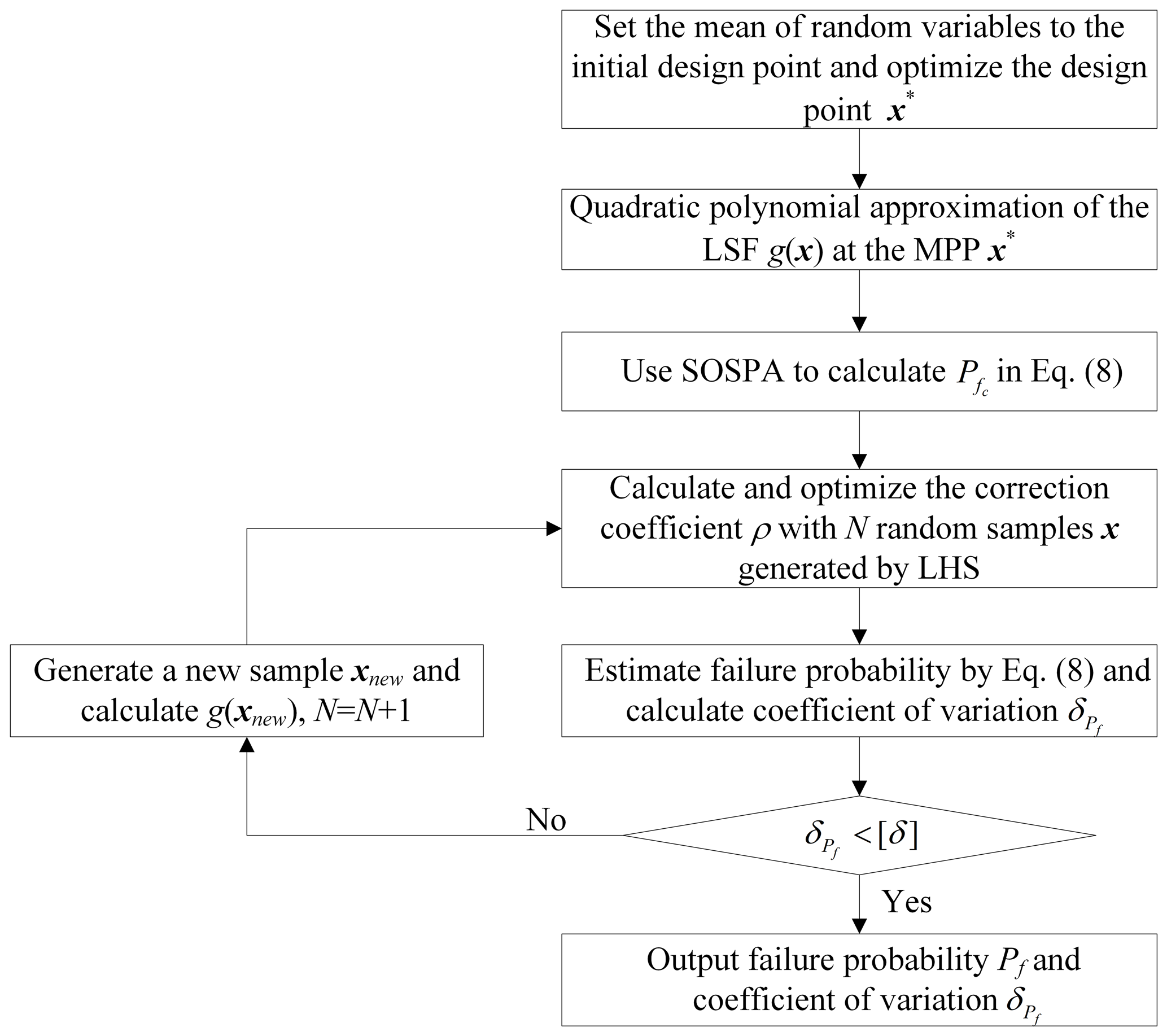
3.2 Procedure of CVLHS with SOSPA

To solve the reliability problem, the procedure to perform the CVLHS with the SOSPA method is shown in Fig. 2. According to the convergence criteria, the threshold value of the coefficient of variation ${\mathit{\delta }}_{P_{f_{\mathrm{CV}}}}$ is set to 0.15–0.25 for different cases in this paper.

Figure 2 The flowchart of the proposed method.

4 Illustrative examples

In this section, four representative examples are provided to demonstrate the accuracy and efficiency of the proposed method in addressing the characteristics of high nonlinearity and complexity in practical engineering problems. These examples include a highly nonlinear numerical problem, a small failure probability problem, and two continuous-system engineering cases. The results obtained from the proposed method, i.e., CVLHS with SOSPA, are compared with those acquired from other methods, including SORM, CVMCS with SOSPA, IS, and MCS. For the IS, the importance sampling density function k_X(x) is selected to have the same form as the PDF f_X(x), with equal means and n times the standard deviation, i.e., μ_k=μ_f and σ_k=nσ_f (where n is set to 2). In four cases, the initial sample size for both CVLHS with SOSPA and CVMCS with the SOSPA methods is set to 10², while, for the MCS method, the initial sample size is 10⁶. To eliminate computational errors, the average of five calculations is taken.

4.1 Highly nonlinear numerical problem

To examine the applicability of the proposed method for the highly nonlinear reliability problem, the LSF with several independent normal random variables is analyzed as follows:

$$\begin{array}{}\text{(31)}& G\left(\mathit{x}\right)=\sum _{i=\mathrm{1}}^{\mathrm{10}}{x}_i^i-{\mathrm{10}}^{\mathrm{8}}.\end{array}$$

The means and standard deviations of the random variables X_i ($i=\mathrm{1},\mathrm{2},\mathrm{\dots },\mathrm{10}$) are all μ_i=10, σ_i=5.

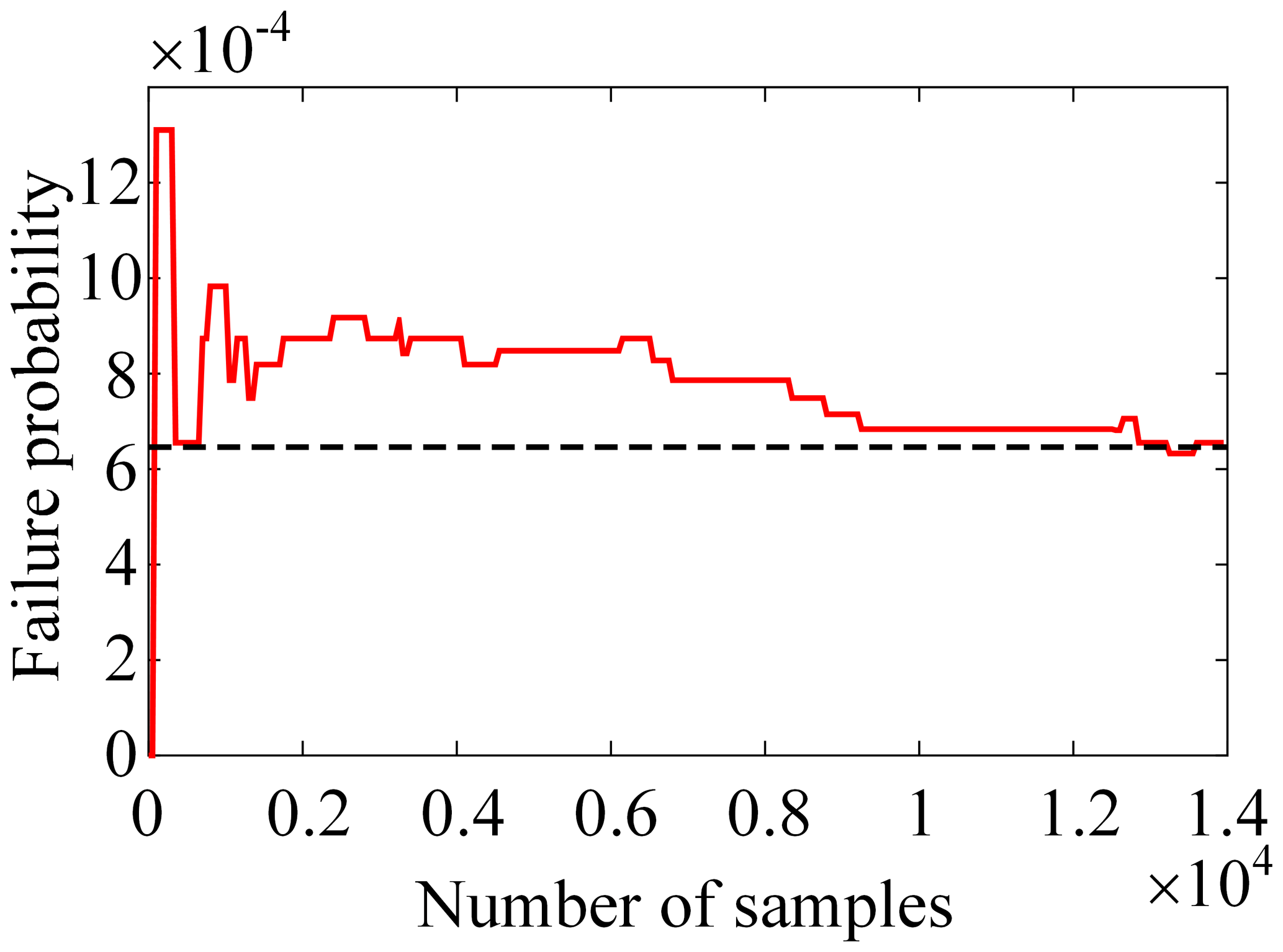
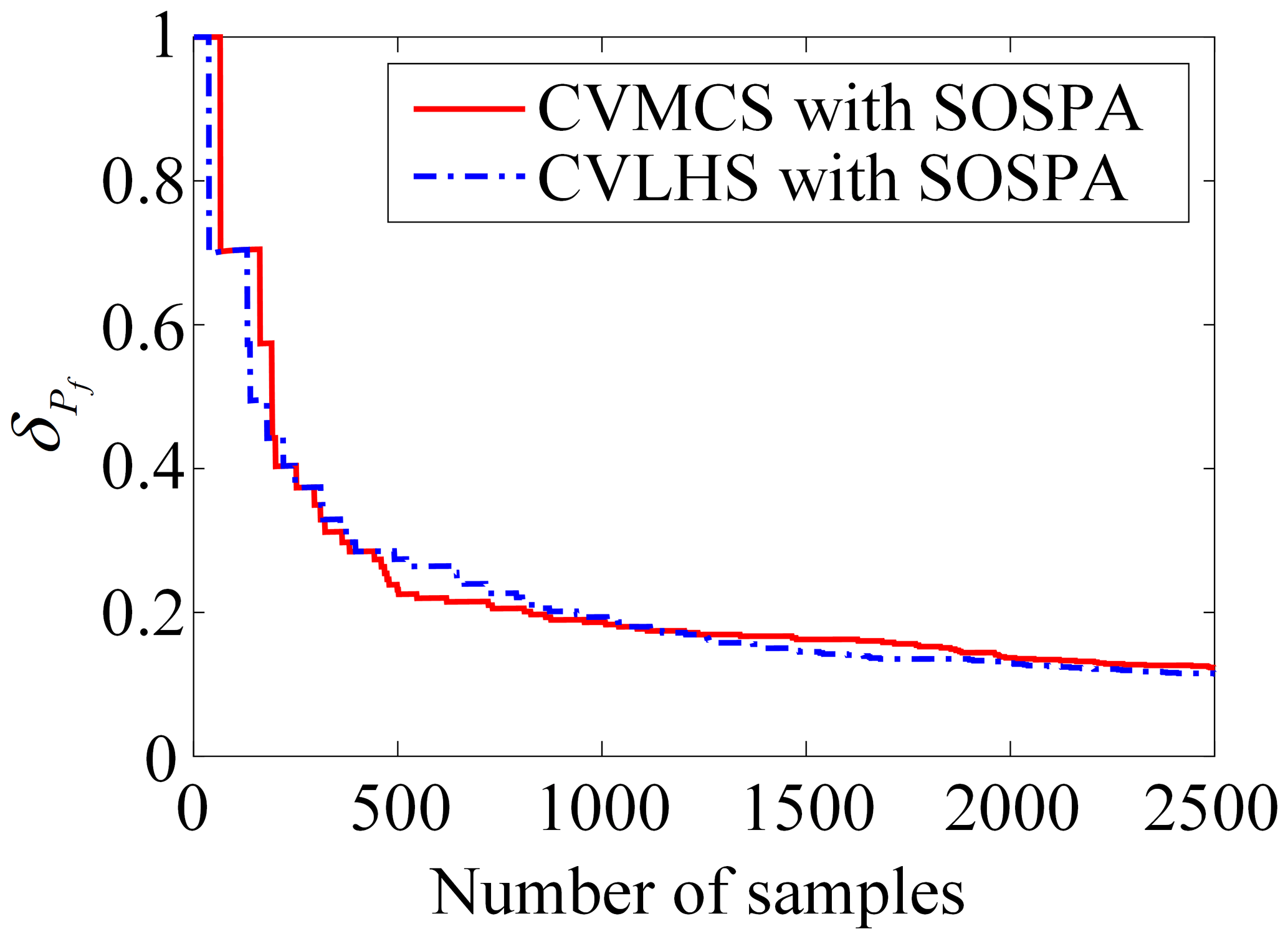
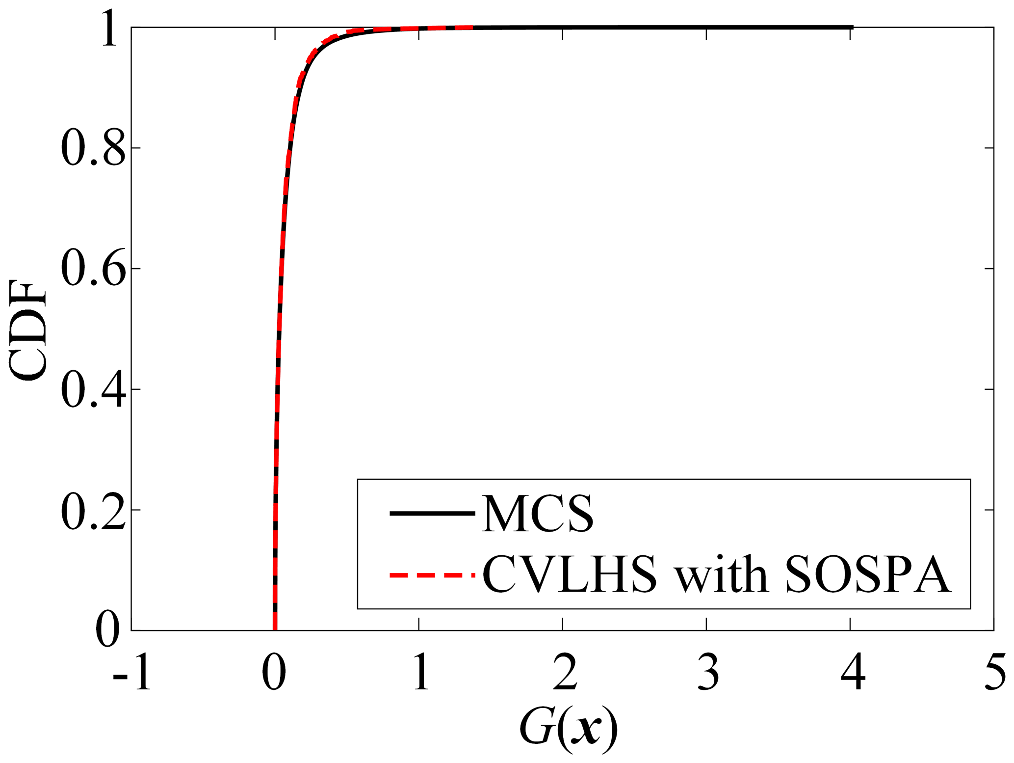
The results of reliability analysis are listed in Table 1. Figure 3 presents the variation curve of the PF by the proposed CVLHS with the SOSPA method with the sample size. Figure 4 compares the convergence procedure of the proposed method and CVMCS with the SOSPA method, and Fig. 5 shows the CDF curves of the LSF by the proposed method and MCS.

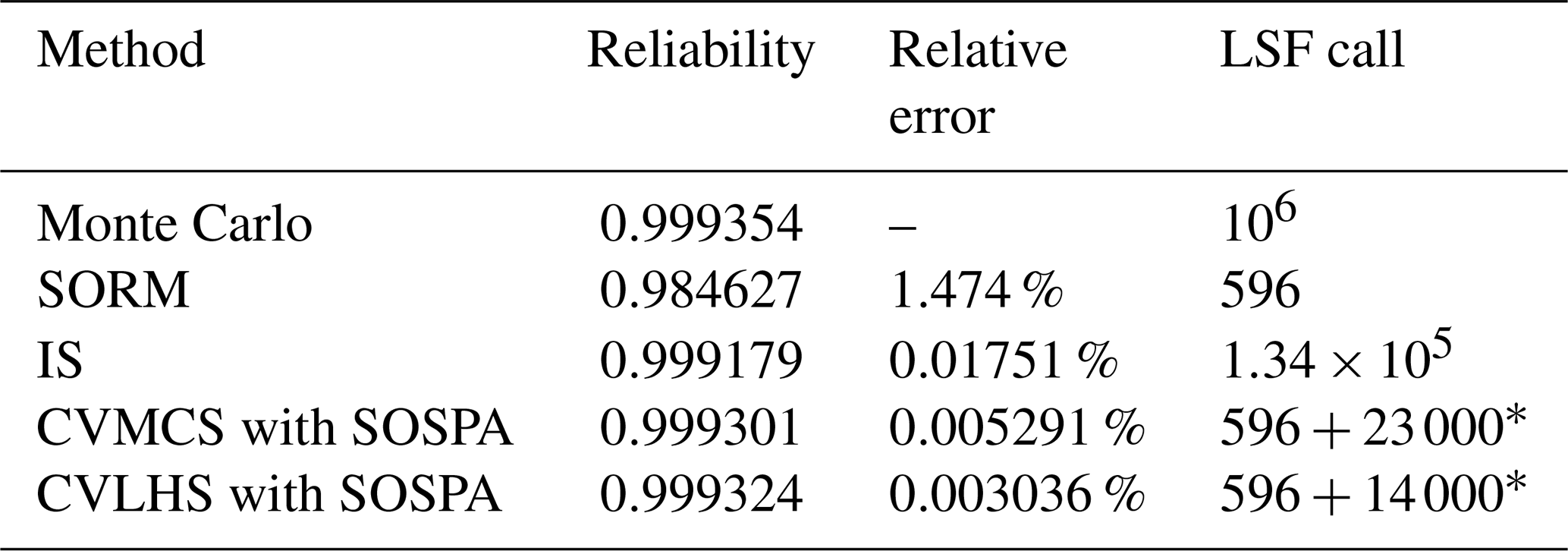
Table 1 Comparison of the results of Example 4.1.

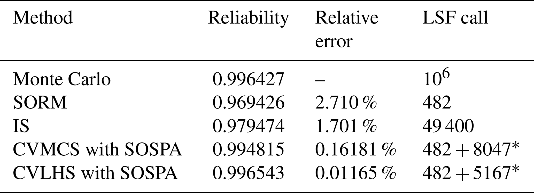
^* LSF call = LSF call(optimize MPP) + LSF call(sampling).

Figure 3 The PF curve by CVLHS with the SOSPA method in Example 4.1.

Figure 4 The curve of the variation coefficient with sample size in Example 4.1.

Figure 5 The CDF of the LSF in Example 4.1.

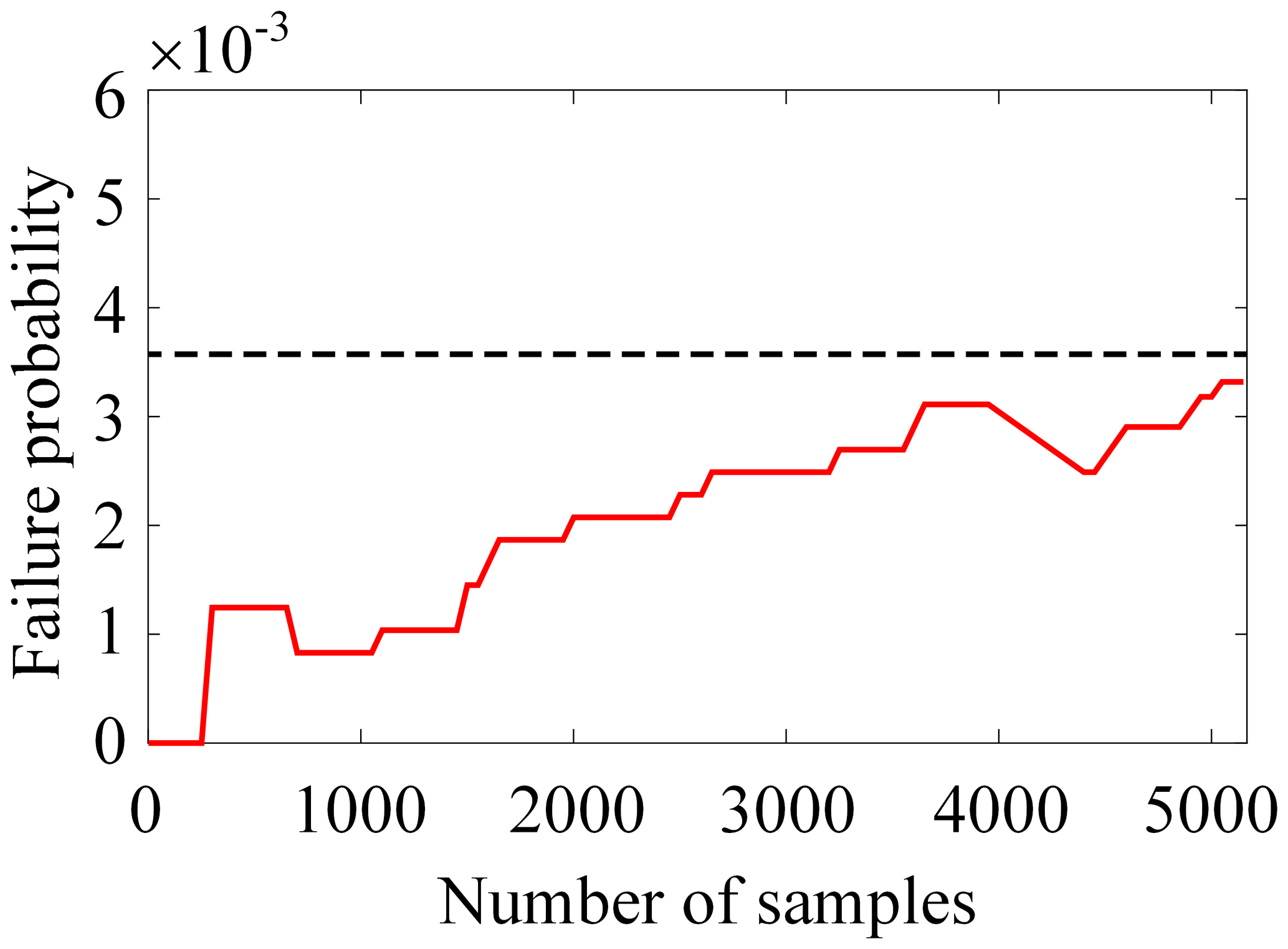
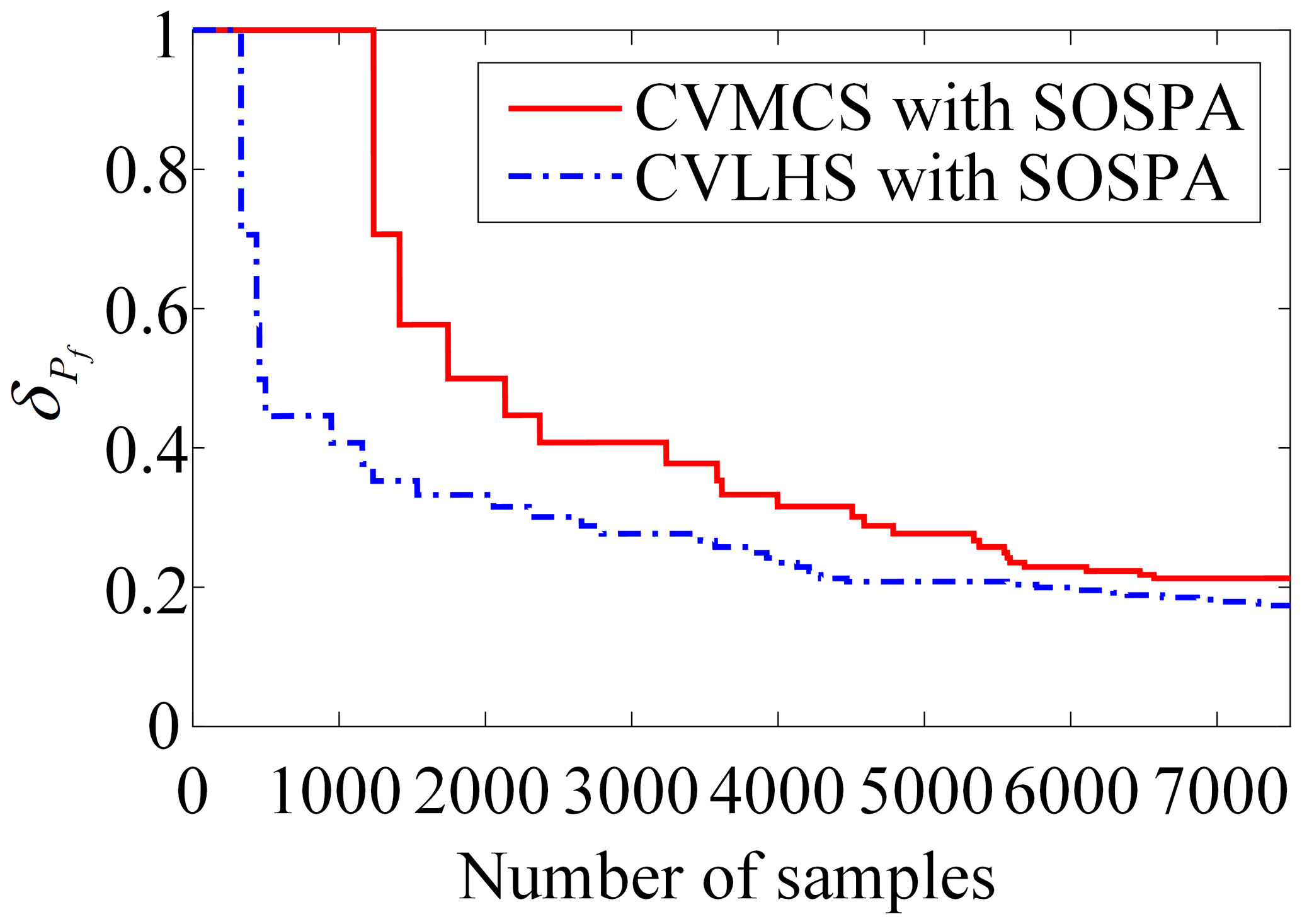
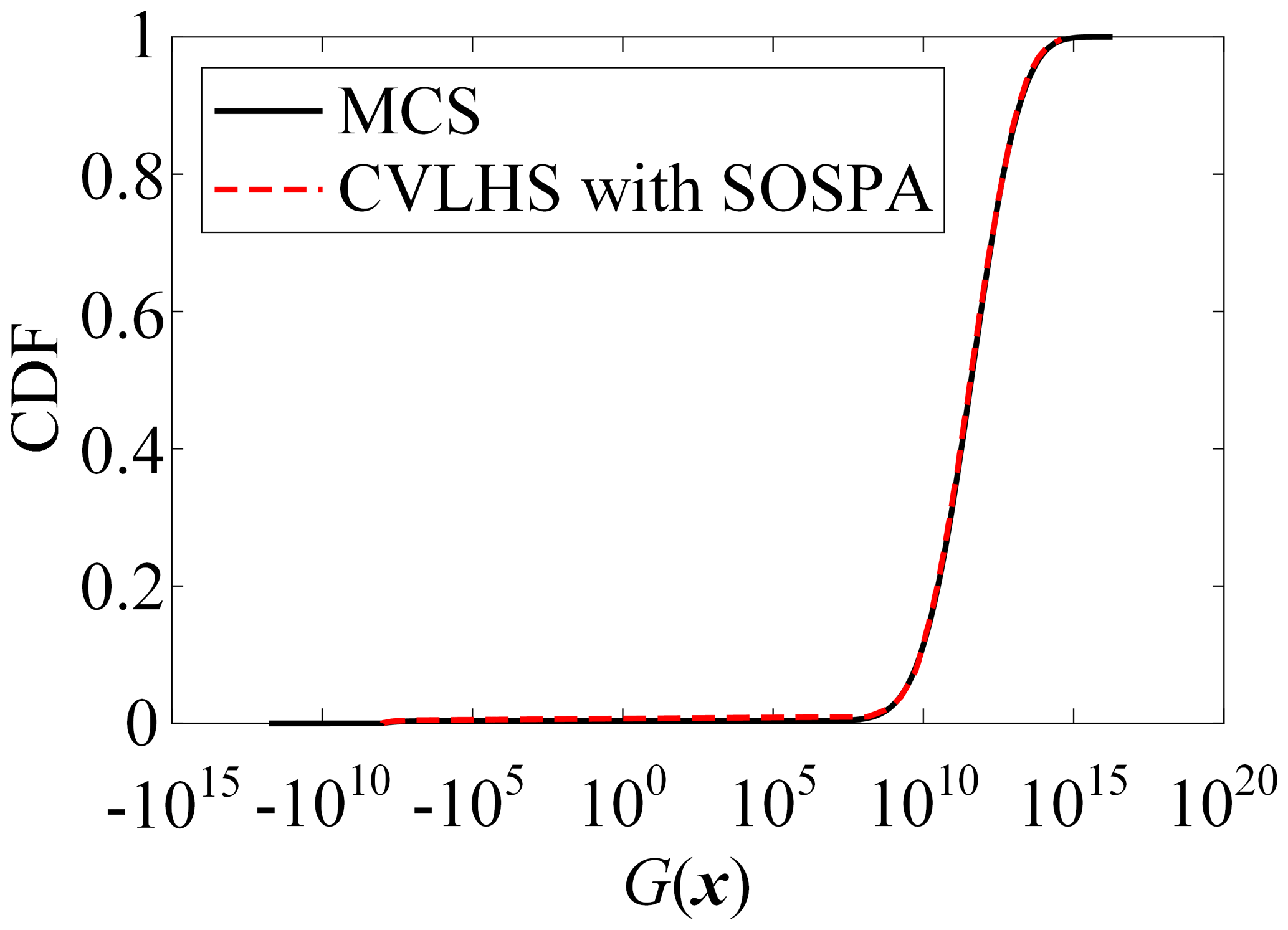
From Table 1, it can be observed that the number of LSF calls is the lowest in SORM among these methods. However, there is a relatively large relative error in the reliability results compared to MCS. IS yields satisfactory results, but it requires a relatively high number of LSF calls. On the other hand, the proposed CVLHS with SOSPA, compared to the CVMCS with SOSPA, further reduces the number of LSF calls while providing more accurate reliability results. In Figs. 3 and 4, both the proposed CVLHS with the SOSPA method and CVMCS with the SOSPA method demonstrate convergence with a small number of samples, with the proposed method converging more quickly and being more efficient. Furthermore, as depicted in Fig. 5, the results obtained from the proposed method closely align with those obtained from MCS. However, the number of LSF calls for the proposed method is merely 0.85 % of that required by MCS. Hence, the proposed CVLHS with the SOSPA method effectively and accurately solves highly nonlinear reliability problems.

4.2 Small failure probability problem

This example illustrates the efficiency and accuracy of the proposed method for the small failure reliability analysis with a high-dimensional LSF. In this example, the LSF, consisting of 40 independent and normally distributed random variables x_i ($i=\mathrm{1},\mathrm{2},\mathrm{\dots },\mathrm{40})\sim N(\mathrm{1.5},\mathrm{1})$, is defined as (Bichon et al., 2008)

$$\begin{array}{}\text{(32)}& G\left(\mathit{x}\right)={\displaystyle \frac{\left(x_{\mathrm{1}}^{\mathrm{2}}+\mathrm{4}\right)\left(x_{\mathrm{2}}-\mathrm{1}\right)}{\mathrm{20}}}-\cos \left({\displaystyle \frac{\mathrm{5}{x}_{\mathrm{1}}}{\mathrm{2}}}\right)+\sum _{i=\mathrm{1}}^{\mathrm{40}}{x}_i^{\mathrm{2}}-\mathrm{71.5}.\end{array}$$

For the small failure probability problem, the results in Table 2 show that the proposed CVLHS with SOSPA, CVMCS with SOSPA, and IS are more accurate than the SORM method. However, in order to achieve the corresponding accuracy, the number of calls to the LSF in IS exceeds 10⁵. Figure 6 demonstrates that the proposed CVLHS with the SOSPA method converges when the sample size reaches 10 000. Additionally, Fig. 7 illustrates the convergence curves of the proposed method and the CVMCS with the SOSPA method, indicating that the proposed method converges at a faster rate. Consequently, the proposed method significantly reduces computational consumption for high-dimensional small failure probability reliability problems. Furthermore, Fig. 8 exhibits strong agreement between the results of the proposed CVLHS with the SOSPA method and those of MCS. However, the number of calls to the LSF for the proposed method is only 1.46 % of that required by MCS. Therefore, it can be verified that the proposed method in this paper significantly reduces the number of calls to the LSF while maintaining accuracy, making it suitable for reliability estimation of problems with small failure probabilities.

Table 2 Comparison of the results of Example 4.2.

^* LSF call = LSF call(optimize MPP) + LSF call(sampling).

Figure 6 The PF curve by CVLHS with the SOSPA method in Example 4.2.

Figure 7 The curve of the variation coefficient with a sample size in Example 4.2.

Figure 8 The CDF of the LSF in Example 4.2.

4.3 Dynamic reliability analysis of a cantilever beam

This example is to verify the accuracy of the proposed CVLHS with the SOSPA method in an engineering structure. The cantilever beam under a dynamic loading F(t) (Bucher, 2009) is shown in Fig. 9. The dynamic motion equation of the cantilever beam is

$$\begin{array}{}\text{(33)}& \mathit{\rho }A{\displaystyle \frac{{\partial }^{\mathrm{2}}\mathit{\omega }}{\partial t^{\mathrm{2}}}}+\text{EI}{\displaystyle \frac{{\partial }^{\mathrm{4}}\mathit{\omega }}{\partial x^{\mathrm{4}}}}=p(x,t),\end{array}$$

where ρ is the constant density, A is the cross-sectional area, and EI is the bending stiffness.

Figure 9 Cantilever beam under dynamic load.

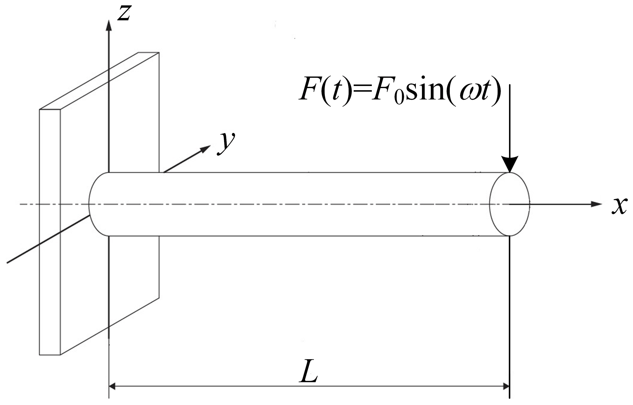
According to the appropriate initial and boundary conditions, the fundamental natural circular frequency ω₁ is given by

$$\begin{array}{}\text{(34)}& {\mathit{\omega }}_{\mathrm{1}}^{\mathrm{2}}={\displaystyle \frac{{\mathit{\lambda }}_{\mathrm{1}}^{\mathrm{4}}\text{EI}}{\mathit{\rho }A}}={\displaystyle \frac{\mathrm{12.362}\text{EI}}{\mathit{\rho }A{L}^{\mathrm{4}}}}.\end{array}$$

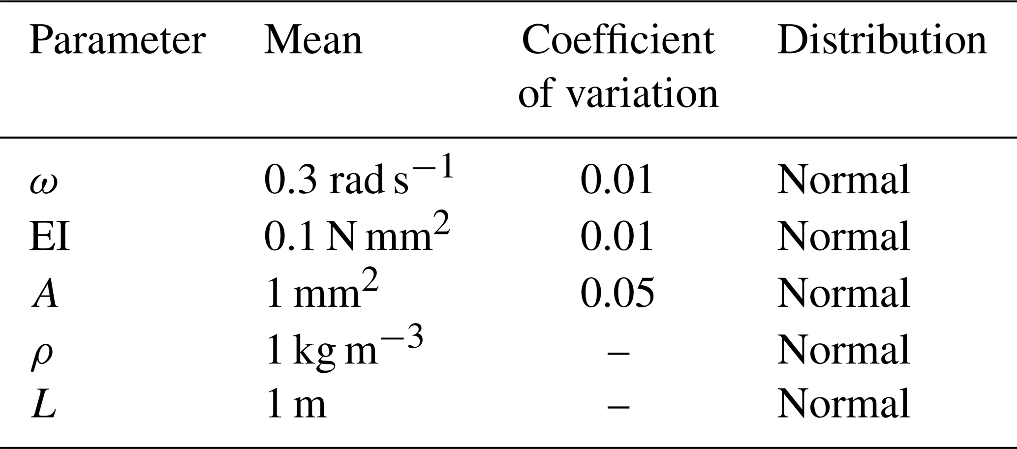
The density and the length are deterministic; i.e., ρ=1 and L=1. The distribution characteristics are shown in Table 3. To avoid resonance failure of the cantilever beam, the ratio is $\mathit{\omega }/{\mathit{\omega }}_{\mathrm{1}}<\mathrm{0.99}$ or $\mathit{\omega }/{\mathit{\omega }}_{\mathrm{1}}>\mathrm{1.01}$.

Table 3 Distribution information of the cantilever beam parameters.

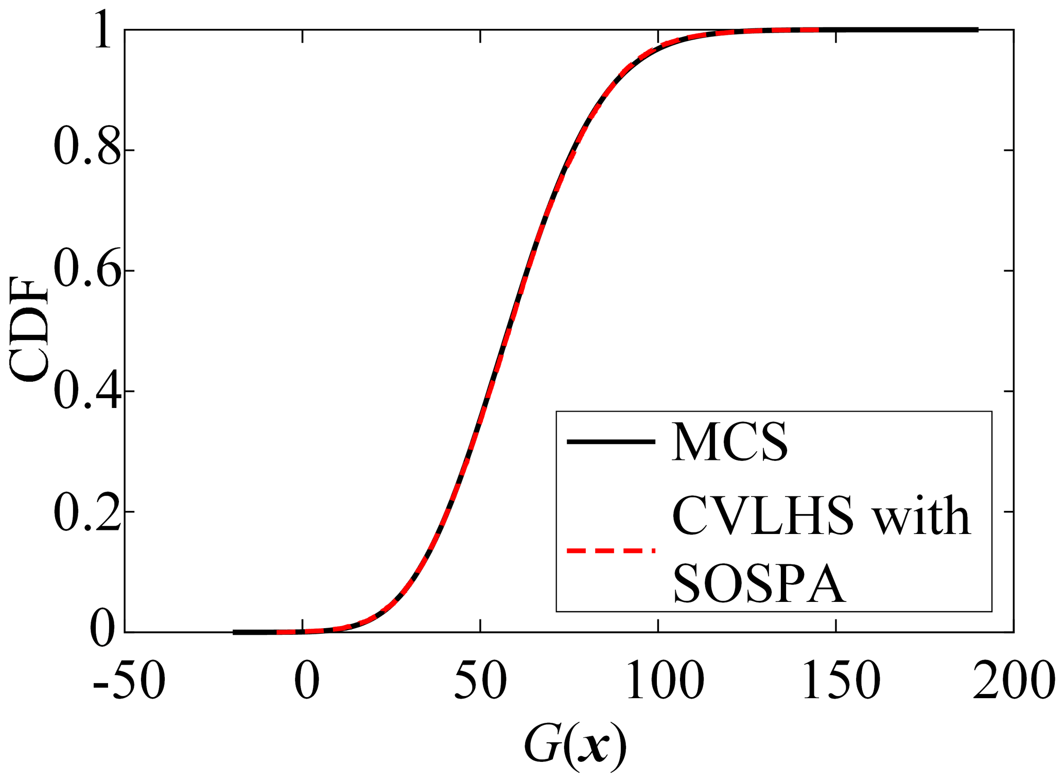
For an engineering structure, as shown in Table 4 and Figs. 10–12, the reliability results of the proposed CVLHS with the SOSPA method fit well with the MCS results, and the relative error is minimal. When the sample size reaches around 1000, the method starts to converge. Compared to the SORM method, the number of calls to the LSF only increased by less than 1300, but the accuracy significantly improved. Compared to the IS method, in order to achieve the corresponding accuracy, the IS requires more than 21 times the number of LSF calls compared to CVLHS with SOSPA.

Table 4 Comparison of the reliability results for the cantilever beam dynamic system.

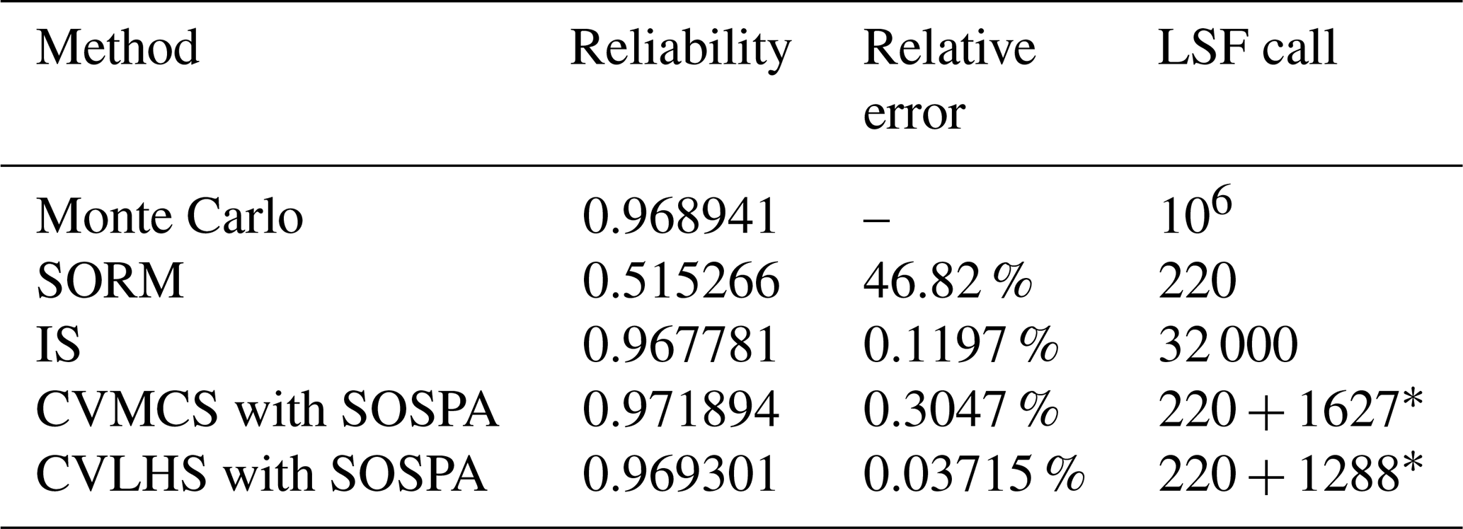
^* LSF call = LSF call(optimize MPP) + LSF call(sampling).

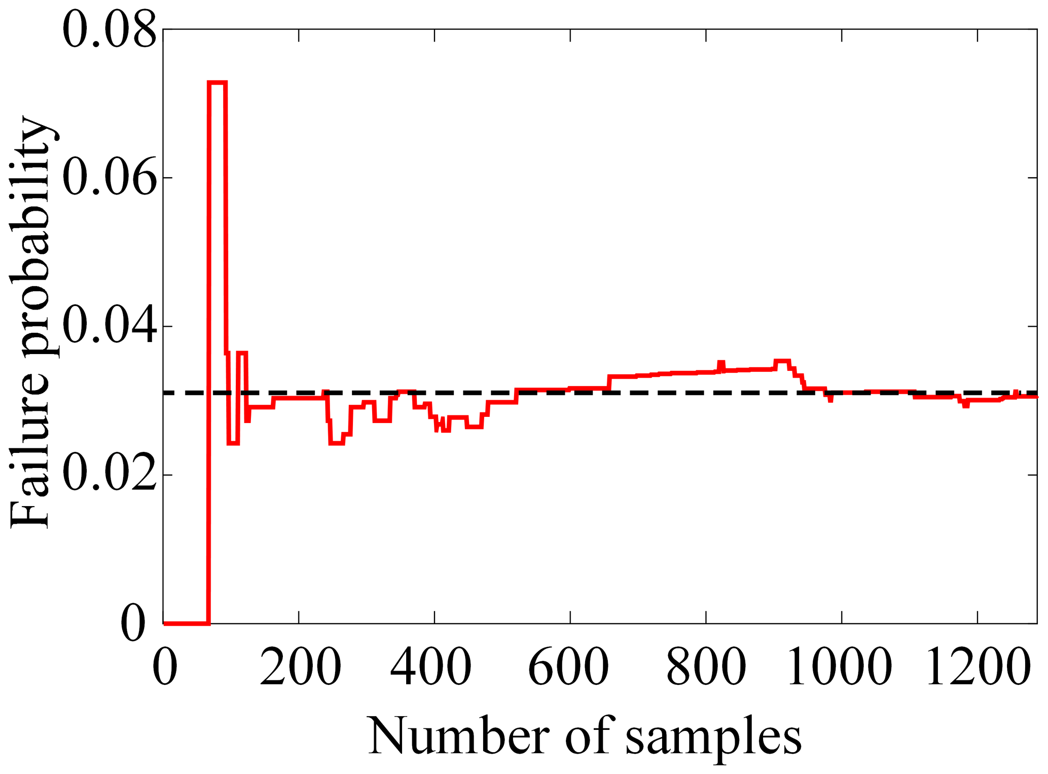
Figure 10 The PF curve by CVLHS with the SOSPA method for the cantilever beam dynamic system.

Figure 11 The curve of the variation coefficient for the cantilever beam dynamic system.

Figure 12 The CDF of the LSF for the cantilever beam dynamic system.

4.4 Reliability of chatter stability in turning

A simplified diagram of a single-degree-of-freedom regenerative chatter dynamics model of the turning process system is shown in Fig. 13.

Figure 13 Dynamic model of cutting regenerative chatter in turning.

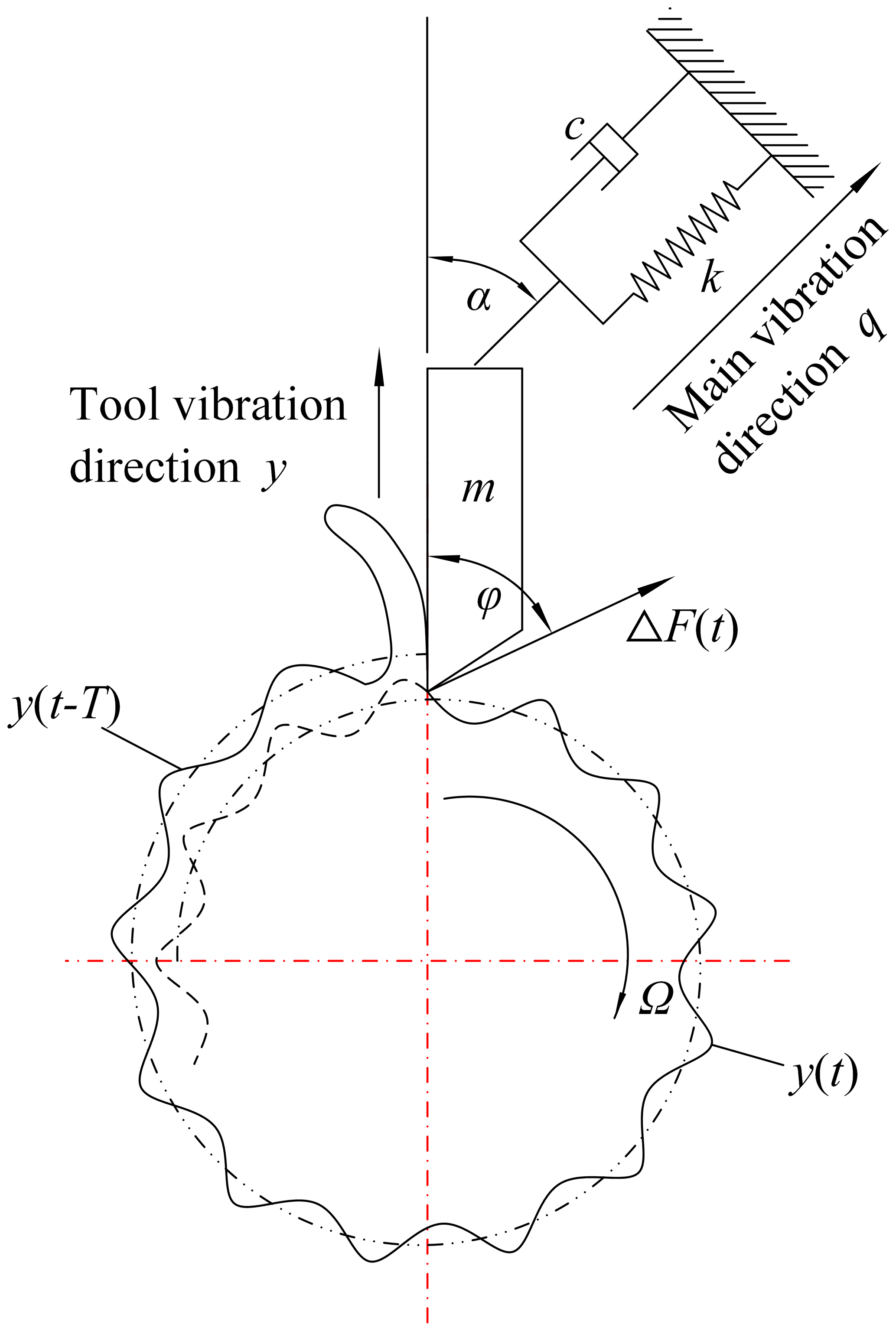
According to the dynamics analysis of the turning process system (Schmitz and Smith, 2009), the limit cutting width is expressed as

$$\begin{array}{}\text{(35)}& \begin{array}{rl}& a_{\mathrm{plim}}={\displaystyle \frac{k\left[{\left(\mathrm{1}-{\mathit{\lambda }}^{\mathrm{2}}\right)}^{\mathrm{2}}+{\left(\mathrm{2}\mathit{\xi }\mathit{\lambda }\right)}^{\mathrm{2}}\right]}{K_{\mathrm{c}}u\left({\mathit{\lambda }}^{\mathrm{2}}-\mathrm{1}\right)}}\\ & \cdot {\displaystyle \frac{\mathrm{1}-\mathit{\eta }\cos \left[\mathrm{2}j\mathit{\pi }+\arcsin \frac{\mathrm{2}\mathit{\xi }\mathit{\lambda }}{\mathit{\eta }\sqrt{{\left(\mathrm{2}\mathit{\xi }\mathit{\lambda }\right)}^{\mathrm{2}}+{\left(\mathrm{1}-{\mathit{\lambda }}^{\mathrm{2}}\right)}^{\mathrm{2}}}}-\arctan \left(\frac{\mathrm{2}\mathit{\xi }\mathit{\lambda }}{\mathrm{1}-{\mathit{\lambda }}^{\mathrm{2}}}\right)\right]}{\mathrm{1}+{\mathit{\eta }}^{\mathrm{2}}-\mathrm{2}\mathit{\eta }\cos \left[\mathrm{2}j\mathit{\pi }+\arcsin \frac{\mathrm{2}\mathit{\xi }\mathit{\lambda }}{\mathit{\eta }\sqrt{{\left(\mathrm{2}\mathit{\xi }\mathit{\lambda }\right)}^{\mathrm{2}}+{\left(\mathrm{1}-{\mathit{\lambda }}^{\mathrm{2}}\right)}^{\mathrm{2}}}}-\arctan \left(\frac{\mathrm{2}\mathit{\xi }\mathit{\lambda }}{\mathrm{1}-{\mathit{\lambda }}^{\mathrm{2}}}\right)\right]}},\end{array}\end{array}$$

and the corresponding spindle speed can be expressed as

$$\begin{array}{}\text{(36)}& \mathrm{\Omega }={\displaystyle \frac{\mathrm{60}\mathit{\lambda }{\mathit{\omega }}_n}{\mathrm{2}j\mathit{\pi }+\arcsin \frac{\mathrm{2}\mathit{\xi }\mathit{\lambda }}{\mathit{\eta }\sqrt{{\left(\mathrm{2}\mathit{\xi }\mathit{\lambda }\right)}^{\mathrm{2}}+{\left(\mathrm{1}-{\mathit{\lambda }}^{\mathrm{2}}\right)}^{\mathrm{2}}}}-\arctan \left(\frac{\mathrm{2}\mathit{\xi }\mathit{\lambda }}{\mathrm{1}-{\mathit{\lambda }}^{\mathrm{2}}}\right)}},\end{array}$$

where ω_n is the natural frequency of the vibration system in turning, ${\mathit{\omega }}_n^{\mathrm{2}}=k/m$, ξ is the damping ratio of the turning system defined as $\mathit{\xi }=c/\mathrm{2}m{\mathit{\omega }}_n$, u is the direction coefficient defined as $u=\cos (\mathit{\phi }-\mathit{\alpha })\cos \mathit{\alpha }$, η is the turning processing overlap coefficient $(\mathrm{0}\le \mathit{\eta }\le \mathrm{1})$, $\mathit{\lambda }=\mathit{\omega }/{\mathit{\omega }}_n$ (vibration frequency ω is slightly larger than the natural frequency ω_n), i.e., λ>1, and $j=\mathrm{0},\mathrm{1},\mathrm{2},\mathrm{\dots }$ is the number of lobes. The cutting force coefficient K_c consists of the tangential cutting force coefficient K_t and the radial cutting force coefficient K_r, and its expression is

$$\begin{array}{}\text{(37)}& K_{\mathrm{c}}=\sqrt{K_{\mathrm{t}}^{\mathrm{2}}+K_{\mathrm{r}}^{\mathrm{2}}}.\end{array}$$

The minimum a_plim appears when chatter is strongest, i.e., η=1, and the first partial derivative of λ in Eq. (35) is taken to obtain the minimum a_plim as

$$\begin{array}{}\text{(38)}& a_{{\mathrm{plim}}_{min}}={\displaystyle \frac{\mathrm{2}k\mathit{\xi }\left(\mathrm{1}+\mathit{\xi }\right)}{K_{\mathrm{c}}u}}.\end{array}$$

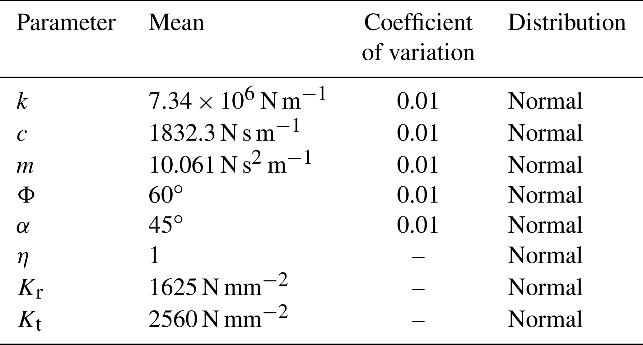
The turning process system would be unstable when the limit cutting width a_plim is not more than the minimum limit cutting width. The distribution characteristics of the turning process parameters are listed in Table 5.

Table 5 Distribution information of the turning process parameters.

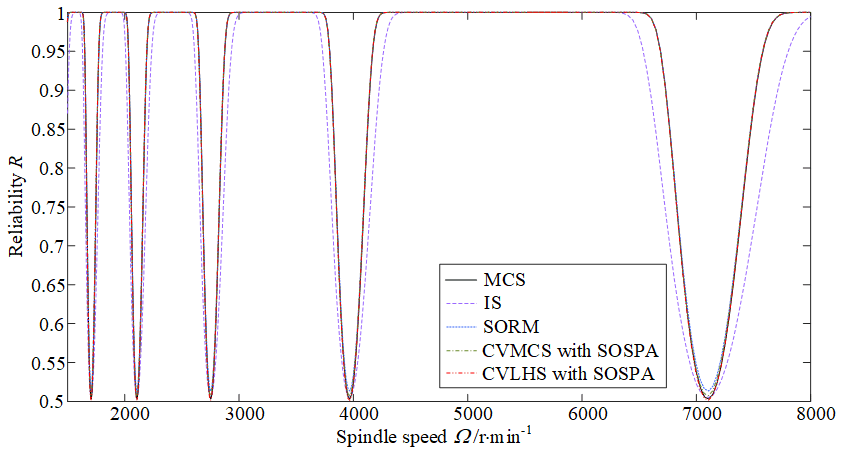
In Fig. 14, the reliability curve of the turning process at different spindle speeds generated by the proposed CVLHS with the SOSPA method is compared with that by SORM, CVMCS with SOSPA, IS and MCS. The results demonstrate that the proposed method achieves the highest consistency with the results obtained by MCS. Therefore, the method has been proven to be feasible for accurately addressing complex practical mechanical engineering reliability problems.

Figure 14 The reliability curve of the chatter stability in turning.

5 Conclusion

To improve the efficiency and accuracy of reliability analysis for engineering systems with high nonlinearity and complexity in practical applications, a novel method is proposed. The method, CVLHS with SOSPA, utilizes CV to transform the original LSF into a highly correlated LSF that can be approximated using SORM. Sample points are generated using LHS, and the probability of failure for the highly correlated LSF is estimated using SPA. The proposed method aims to reduce the number of function calls required by simulation method that employ variance reduction technique, by integrating approximate analytical method.

Through the reliability analysis of the examples, it is evident that the proposed method achieves accurate approximation of the failure probability with a reasonable number of samples, whereas MCS and IS require a large number of samples to achieve the desired level of accuracy. Additionally, when the relative error of the reliability calculation results obtained by SORM is relatively high, the proposed method still provides accurate estimation with a reasonable sample size. The results demonstrate that, for complex nonlinear problems, the proposed method requires less than 1.5 % of the LSF calls compared to MCS while maintaining a high level of accuracy. Moreover, the comparison between CVLHS with SOSPA and CVMCS with SOSPA results reveals that, even in situations where a large number of samples cannot be utilized in the modeling process, which is often a concern in practical engineering, CVLHS with SOSPA can accurately predict the failure probability using a small number of initial samples generated by LHS, thus further reducing the required number of LSF calls. Hence, the proposed method significantly reduces the number of LSF calls while ensuring high-precision reliability results.

While the proposed method in this study combines the advantages of an approximate analytical method and a simulation method, it is suitable for engineering problems where an explicit limit state function can be established. To further investigate and expand this method, the integration of surrogate model methods can be considered, and the reliability analysis results can be compared to identify the optimal integration approach.