Optimal resource allocation method and fault-tolerant control for redundant robots

Resource coordination and allocation strategies are proposed to reduce the probability of failure by aiming at the problem that the robot cannot continue to work after joint failure. Firstly, the principal component analysis method under unsupervised branches in machine learning is used to analyze the reliability function and various indexes of the robot to obtain the comprehensive evaluation function. Then, based on the fault-tolerant-control inverse-kinematics optimal algorithm, each joint can be scheduled by weighted processing. Finally, the comprehensive evaluation function is used as an index to evaluate the probability of fault occurrence, and the weight is defined to realize the coordinated resource allocation of redundant robots. Taking the planar four revolute joints (4R) redundant robot as an example, the algorithm control is compared. Based on reasonable modeling and physical verification, the results show that the method of optimal resource coordination and allocation is effective.

1 Introduction

As the cross-discipline of robotics has flourished, it has become a major player in the agricultural sector. However, robot components can age over time or have sudden changes in load, leading to robot failure, and according to robot maintenance staff, when robots fail, they are shut down for repair, which undoubtedly increases time costs. In actual agricultural production, some fruits have a very short picking cycle, for example, cherries, which are picked in half a month, and if they are not picked in time, they will cause economic losses. It is common for crops with a short picking cycle to be picked a little early and then ripened, but this method requires good ventilation to avoid accumulating too much moisture and mold, and the ripened fruit is not as good in taste and flavor as tree-ripened fruit. In order to ensure that the robot picks the fruit at the optimum time, it needs to be able to operate even if it experiences a joint malfunction, avoiding financial losses due to maintenance and missing the optimum picking time. To meet these requirements, the robot must be highly reliable and fault tolerant. Fault-tolerant operation reduces its downtime and can also be used to extend its service life or to detect subsystem failures early and speed up the repair process. Fault tolerance in redundant robots has therefore become a major focus of attention.

The most systematic and in-depth research on fault-tolerant control of redundant robotic arms is conducted by the group of Ahmad A. Almarkhi and Khaled M. Ben-Gharbia and Anthony A. Maciejewski, whose research ranges from fault-tolerant control of planar three-joint redundant machines to fault-tolerant control of spatially redundant robotic arms, proposing the design of optimal fault-tolerant Jacobi matrices and maximizing the size of a self-moving human face to improve the fault tolerance of the robot and for optimal fault tolerance for different joint failure probabilities. Many original contributions to the design of robot kinematics have been made (Ben-Gharbia et al., 2014; Xie and Maciejewski, 2017, 2018; Almarkhi and MacIejewski, 2019; Almarkhi et al., 2020). Abdi and Nahavandi (2012) proposed the theory of optimal fault-tolerant configurations using condition numbers as optimization terms. Many domestic scholars have also researched fault-tolerant control of redundant manipulators. Jing Zhao's Beijing University of Technology team has conducted in-depth research on this aspect. They have proposed a series of control algorithms for redundant robotic arms, flexible redundant robotic arms, and robot coordination and verified the effectiveness of these algorithms through experiments (Xie and Zhao, 2010a; Zhao et al., 2014, 2012; Xie and Zhao, 2010b). Jia Qingxuan's Beijing University of Posts and Telecommunications team has researched multi-joint and multi-type fault-tolerant control, global fault-tolerant trajectory optimization methods, and joint velocity mutation suppression during force and/or position fault tolerance and verified the accuracy of the algorithms through examples. Changchun Liang from the General Design Department of Beijing Space Vehicles studied the space robotic arm using a degenerate Jacobi-matrix-based mutation suppression method and made control simulations for three operating conditions: pre-failure, operation, and post-failure suppression (Liang et al., 2016). Zhaohui Zhu from the Beijing University of Technology analyzed the seven rotating joints (7R) redundant robotic arm, from the working space of fault-tolerant performance to the screening of fault-tolerant dislocations by comprehensive indicators (Zhu, 2016). Yu Cao, Southeast University, conducted a fault tolerance analysis of an anthropomorphic redundant robot arm with joint bias and made a prototype for the algorithm's effectiveness (Cao, 2019). Yanhui Wei, Harbin Engineering University, conducted a study on the fault tolerance of reconfigurable-robot working configurations and verified the effectiveness of the fault tolerance analysis method and the feasibility of the fault tolerance control method through example validation (Wei et al., 2010). Yu She, Harbin Institute of Technology, conducted a study on the kinematics and control of a redundant robot with a single joint. The kinematics and dynamics of a single-joint robot are re-modeled, and the trajectory planning under single-joint failure is investigated (She, 2013), Bo Zhao of Jilin University conducts an active decentralized fault-tolerant control method for reconfigurable robots with multiple concurrent faults and conducts an in-depth study from the field of control (Zhao, 2014). Minghao Li of Southwest University of Science and Technology adopts a deep reinforcement learning approach to fault-tolerant control of robotic arms and does experiments to verify the algorithm's effectiveness (Li, 2019; Li and Zhang, 2020). Nie Fu Jie of Changchun University of Technology conducted a decentralized optimal active fault-tolerant control for reconfigurable robotic arms based on an adaptive dynamic programming approach (Nie, 2021). Bing Ma of Changchun University of Technology obtained a decentralized near-optimal fault-tolerant controller with an observation–compensation–evaluation network structure (Ma, 2021).

From the above, it can be seen that, at present, most of the research in the field of fault-tolerant control is directed toward fault-tolerant control after a fault has occurred, such as suppressing sudden changes in joint speed and suppressing sudden changes in torque. Although the end position and end speed are guaranteed not to change abruptly, the joint speed will change abruptly, which leads to great instantaneous acceleration of the joint and easy damage to the motor. Based on a real-time control method for the optimal total performance of a planar redundant robot (Rong et al., 2022), this paper proposes a control method for optimal coordinated resource allocation of a redundant robot and is structured as follows: this paper introduces the concept of coordinated resource allocation, derives a comprehensive evaluation function based on the robot indicators and reliability functions through principal component analysis, and thus carries out coordinated resource allocation control based on this comprehensive evaluation function. The core of the algorithm is based on the comprehensive evaluation function for all tracking points in the trajectory. The comprehensive evaluation function is used to define the weight of the joint that affects the performance the most, to reduce the degree of impact on the overall performance after the failure of the joint, to reduce the sudden change in the angle of each joint when a failure occurs, and to achieve a smooth transition between the speed of the joint before the failure and the speed of the joint after the failure.

2 Robot reliability curve

The most fundamental analytical methods in reliability studies are probability distributions, of which four are considered to be useful in the study of the reliability and safety of robotic systems, namely (i) exponential distribution, (ii) Rayleigh distribution, (iii) Weibull distribution, and (iii) bathtub hazard rate curve distribution (Dhillon, 2015). It has been shown that the failure rate of most robots is a function of time, with the most commonly used being the bathtub hazard rate curve. The distribution is like the shape of a bathtub.

The bathtub hazard rate curve function equation is

$$\begin{array}{}\text{(1)}& \mathit{\lambda }\left(t\right)=\mathit{\theta }a(\mathit{\theta }t{)}^{a-\mathrm{1}}{e}^{(\mathit{\theta }t{)}^a},\end{array}$$

where t is time, λ(t) is the hazard rate, a is the shape parameter, and θ is the scale parameter.

The hazard rate function can also be expressed as

$$\begin{array}{}\text{(2)}& \mathit{\lambda }\left(t\right)={\displaystyle \frac{f\left(t\right)}{R\left(t\right)}}.\end{array}$$

R(t) is the general reliability function, and f(t) is the fault density function.

The fault density function is related to the hazard rate function as follows:

$$\begin{array}{}\text{(3)}& f\left(t\right)=-{\displaystyle \frac{\mathrm{d}R\left(t\right)}{\mathrm{d}t}}.\end{array}$$

From the above equation, it can be deduced that

$$\begin{array}{}\text{(4)}& -\mathit{\lambda }\left(t\right)\mathrm{d}t=-{\displaystyle \frac{\mathrm{1}}{R\left(t\right)}}\cdot \mathrm{d}R\left(t\right).\end{array}$$

By integrating both sides of the equation, we get the following formula:

$$\begin{array}{}\text{(5)}& -{\int }_{\mathrm{0}}^t\mathit{\lambda }\left(t\right)\mathrm{d}t={\int }_{\mathrm{1}}^{R\left(t\right)}{\displaystyle \frac{\mathrm{1}}{R\left(t\right)}}\cdot \mathrm{d}R\left(t\right),\end{array}$$

where, when t=0, $R\left(t\right)=\mathrm{1}.$

$$\begin{array}{}\text{(6)}& \ln R\left(t\right)=-{\int }_{\mathrm{0}}^t\mathit{\lambda }\left(t\right)\mathrm{d}t\end{array}$$

Thus from the above equation, we have

$$\begin{array}{}\text{(7)}& R\left(t\right)=e^{-{\int }_{\mathrm{0}}^t\mathit{\lambda }\left(t\right)\mathrm{d}t}.\end{array}$$

Therefore, we can obtain the reliability function of the probability distribution of the failure time of the system. By substituting Eq. (2) into Eq. (7) for calculation, the reliability function of the bath curve is

$$\begin{array}{}\text{(8)}& R\left(t\right)=e^{-{\int }_{\mathrm{0}}^t\mathit{\left\{}\mathit{\theta }a\right(\mathit{\theta }t{)}^{a-\mathrm{1}}{e}^{(\mathit{\theta }t{)}^a}\mathit{\}}\mathrm{d}t}=e^{-\mathit{\{}{e}^{(\mathit{\theta }t{)}^a}-\mathrm{1}\mathit{\}}}.\end{array}$$

Equation (8) shows that the reliability of the robot decreases when the robot uses the bathtub curve as a hazard function, which is also in line with the actual production pattern. This reliability function can therefore be used as an indicator to analyze the robot's performance.

3 Principal component analysis

Principal component analysis (PCA) is an important evaluation method for quantitative calculations, which allows instantaneous planar data to be replaced by a small number of integrated variables with minimal loss of information from the original data, making the data structure much simpler. The data structure can be greatly simplified.

These attempts to integrate the reliability function and multiple evaluation indicators of the robot using the PCA method, from which a comprehensive evaluation function is derived, provide the basis for an optimal control method for the coordinated allocation of resources.

The principal component analysis method is divided into two main aspects in this paper: firstly, the establishment of a comprehensive evaluation index consisting of a reliability function and the fusion of several evaluation indicators of the robot, and secondly, the determination of the relevance of every single indicator according to the correlation coefficient matrix. The main steps are outlined below.

• 1.

  The data are standardized for all indicators to resolve the original problem of inconsistencies in the data scale, thus enabling standardized data for further evaluation.

  Let the matrix of indicators be composed of m experimental samples and n indicators.

  $$\begin{array}{}\text{(9)}& \mathbf{X}={\left(\begin{array}{cccc}{x}_{\mathrm{11}}& x_{\mathrm{12}}& \mathrm{⋮}& x_{\mathrm{1}n}\\ x_{\mathrm{21}}& x_{\mathrm{22}}& \mathrm{⋮}& x_{\mathrm{2}n}\\ \mathrm{\cdots }& \mathrm{\cdots }& \mathrm{\ddots }& \mathrm{\cdots }\\ x_{m\mathrm{1}}& x_{m\mathrm{2}}& \mathrm{⋮}& x_{mn}\end{array}\right)}_{m\times n}\end{array}$$

  The Z-score transform was used to normalize X. The normalization equation is

  $$\begin{array}{}\text{(10)}& Z_{ij}=\left(x_{ij}-\stackrel{\mathrm{‾}}{x_j}\right)/S_j,\end{array}$$
  $$\begin{array}{}\text{(11)}& \stackrel{\mathrm{‾}}{x_j}=\sum _{i=\mathrm{1}}^m{x}_{ij}/m{S}_j^{\mathrm{2}}=\sum _{i=\mathrm{1}}^m{\left(x_{ij}-\stackrel{\mathrm{‾}}{x_j}\right)}^{\mathrm{2}}/\left(m-\mathrm{1}\right).\end{array}$$

  The normalization matrix is then obtained as follows:

  $$\begin{array}{}\text{(12)}& \mathbf{Z}=\left(z_{ij}\right)={\left(\begin{array}{cccc}{z}_{\mathrm{11}}& z_{\mathrm{12}}& \mathrm{\cdots }& z_{\mathrm{1}n}\\ z_{\mathrm{21}}& z_{\mathrm{22}}& \mathrm{\cdots }& z_{\mathrm{2}n}\\ \mathrm{⋮}& \mathrm{⋮}& \mathrm{\ddots }& \mathrm{⋮}\\ z_{m\mathrm{1}}& z_{m\mathrm{2}}& \mathrm{\cdots }& z_{mn}\end{array}\right)}_{m\times n}.\end{array}$$
• 2.

  The correlation coefficient R is calculated. Since there may be some correlation between single indicators, making the data have some information overlap, applying the correlation coefficient matrix can fully reflect the correlation between these indicators, which is also the primary condition for dimensionality reduction. The correlation coefficient matrix R is expressed as follows:

  $$\begin{array}{}\text{(13)}& \mathbf{R}={\displaystyle \frac{\mathrm{1}}{n-\mathrm{1}}}{\mathbf{Z}}^T\mathbf{Z},\end{array}$$

  where R is a matrix of order n×n, and Z^T is the transpose matrix of the matrix Z.

• 3.

  The eigen roots and eigenvectors of the correlation coefficient matrix R are calculated. From the equation $\mathrm{|}\mathit{\lambda }\mathbf{E}-\mathbf{R}\mathrm{|}=\mathrm{0}$, n eigenvalues are obtained in ascending order, ${\mathit{\lambda }}_{\mathrm{1}}\ge {\mathit{\lambda }}_{\mathrm{2}}\ge \mathrm{\dots }\ge {\mathit{\lambda }}_n\ge {\mathit{\lambda }}_{\mathrm{0}}$.

  The eigenvector corresponding to the n eigen roots is obtained from the system of equations $\mathrm{|}\mathit{\lambda }\mathbf{E}-\mathbf{R}\mathrm{|}\mathbf{X}=\mathrm{0}$ as

  $$\begin{array}{}\text{(14)}& \mathbf{ZX}=\left(\begin{array}{c}{\mathbf{ZX}}_{\mathrm{1}}\\ {\mathbf{ZX}}_{\mathrm{2}}\\ \mathrm{⋮}\\ {\mathbf{ZX}}_n\end{array}\right),\end{array}$$

  where ZX_i corresponds to the eigenvalue λ_i unit and the eigenvector ${\mathbf{ZX}}_i=\left({\mathbf{ZX}}_{\mathrm{1}i},{\mathbf{ZX}}_{\mathrm{2}i},\mathrm{\cdots },{\mathbf{ZX}}_{ni}\right)$.

• 4.

  The number of principal components is determined. In this paper, the number of principal components of the comprehensive evaluation indexes is determined by the cumulative variance contribution of each index and the reliability function, i.e., according to the proportion of variance in relation to the total variance.

  $$\begin{array}{}\text{(15)}& \mathit{\alpha }=\sum _{i=\mathrm{1}}^p{\mathit{\lambda }}_i/\sum _{i=\mathrm{1}}^n{\mathit{\lambda }}_i\end{array}$$

  For research, a cumulative contribution rate of 50 % is acceptable, and more than 70 % can be used as the standard for practical application. However, in order to be more relevant, α≥ 85 % is usually taken to select the number of p as the main component.

• 5.

  We can get the expression for the principal component $F_i(i=\mathrm{1},\mathrm{2},\mathrm{\dots },p)$ as follows:

  $$\begin{array}{}\text{(16)}& \begin{array}{rl}& F_i=\mathbf{Z}\times \mathbf{Z}{X}_i\\ & =\left(\begin{array}{c}{z}_{\mathrm{11}}\mathbf{Z}{X}_{\mathrm{1}i}+z_{\mathrm{12}}\mathbf{Z}{X}_{\mathrm{2}i}+\mathrm{\cdots }+z_{\mathrm{1}n}\mathbf{Z}{X}_{ni}\\ z_{\mathrm{21}}\mathbf{Z}{X}_{\mathrm{1}i}+z_{\mathrm{22}}\mathbf{Z}{X}_{\mathrm{2}i}+\mathrm{\cdots }+z_{\mathrm{2}n}\mathbf{Z}{X}_{ni}\\ \mathrm{⋮}\\ z_{m\mathrm{1}}\mathbf{Z}{X}_{\mathrm{1}i}+z_{m\mathrm{2}}\mathbf{Z}{X}_{\mathrm{2}i}+\mathrm{\cdots }+z_{mn}\mathbf{Z}{X}_{ni}\end{array}\right).\end{array}\end{array}$$
• 6.

  The comprehensive evaluation function is determined.

  $$\begin{array}{}\text{(17)}& \begin{array}{rl}F& ={\displaystyle \frac{{\mathit{\lambda }}_{\mathrm{1}}}{{\mathit{\lambda }}_{\mathrm{1}}+{\mathit{\lambda }}_{\mathrm{2}}+\mathrm{\dots }{\mathit{\lambda }}_p}}{F}_{\mathrm{1}}\\ & +{\displaystyle \frac{{\mathit{\lambda }}_{\mathrm{1}}}{{\mathit{\lambda }}_{\mathrm{1}}+{\mathit{\lambda }}_{\mathrm{2}}+\mathrm{\dots }{\mathit{\lambda }}_p}}{F}_{\mathrm{2}}\\ & +\mathrm{\dots }+{\displaystyle \frac{{\mathit{\lambda }}_p}{{\mathit{\lambda }}_{\mathrm{1}}+{\mathit{\lambda }}_{\mathrm{2}}+\mathrm{\dots }{\mathit{\lambda }}_p}}{F}_p\end{array}\end{array}$$

4 Robotic-arm indicators

Commonly used single performance indicators for robotic arms consist of kinematic condition number (x₁) (Klein and Blaho, 1987), kinematic maneuverability (x₂) (Yoshikawa, 1985), isotropic indicators (x₃) (Mayorga et al., 2005), other indicators (x₄) (Xie and Zhao, 2010a), and reliability (x₅) (Dhillon, 2015). Specific information on each single performance indicator is given in Table 1.

Table 1 Common performance indicators.

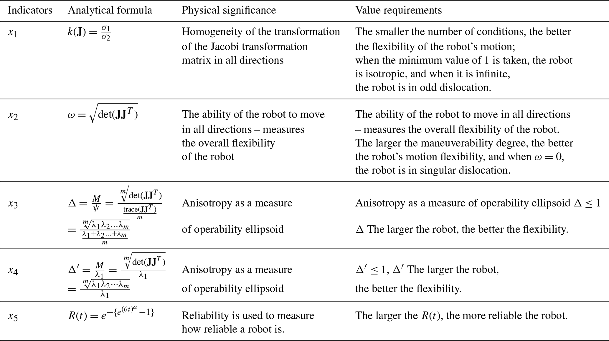
Note: λ_m is the eigenvalue of the matrix JJ^T.

5 Optimal-redundancy inverse-solution algorithm under fault-tolerant control

Let us assume we have a redundant robot with n degrees of freedom and m absolute end motion parameters and a robot redundancy of $r=n-m$. When a joint of the robot fails and locks, the original robot motion will change to that of the degraded robot, and as that joint fails and locks, the structure of the Jacobi matrix will change, and the velocities of the remaining joints will be redistributed. This will result in a difference between the velocity of the original robot arm joint and the velocity of the degraded robot arm joint. Therefore, we define it as the robot joint velocity jump (JVJ), and the mathematical expression is as follows:

$$\begin{array}{}\text{(18)}& {}^i{\mathit{\lambda }}_j=\left|{}^i{\dot{\mathit{\theta }}}_j-{\dot{\mathit{\theta }}}_j\right|,\text{(19)}& {\displaystyle }\text{s.t.}\mathbf{j}\ne \mathbf{i},\text{(20)}& {\displaystyle }\text{If}\mathbf{i}<\mathbf{j},\text{let}{}^i{\dot{\mathit{\theta }}}_j={}^i{\dot{\mathit{\theta }}}_{j-\mathrm{1}},\end{array}$$

where ⁱλ_j is the vector of sudden changes in velocity for each of the remaining joints of the robot after a failure of any one during the entire operation. ${\dot{\mathit{\theta }}}_j$ is the velocity vector of each joint of the original robot. ${}^i{\dot{\mathit{\theta }}}_j$ is the velocity vector for each joint of the degraded robot.

In the above formula, the variable of angular velocity subscript j ranges from 1 to n, and the variable j represents which robot joint it belongs to; the superscript i indicates the faulty joint, and the meaning of Eq. (19) excludes the faulty joint vector from the velocity vector of each joint of the robot after degradation when the i joint fails.

For the jumping of robot joint speed, its essence is that the structure of the Jacobian matrix in the normal working environment is different from that in the fault environment, which leads to the jumping of robot joint speed. Although the end position of the robot does not change, the speed of the robot joint will also jump. Therefore, just avoiding the singularity of the Jacobian matrix after robot failure cannot really reduce the speed jump of robot locking joints.

In this paper, the robot joint failure is defined as the locking-joint failure so the redundant robot will face the following three problems when carrying out the fault-tolerant operation: (1) maintaining the maximum operability of the robot to ensure that, when the robot joint fails, it will try to avoid the singular position; (2) ensuring that the task is as close to the center as possible to ensure that the robot end effector can always carry out work tasks in the fault-tolerant workspace; (3) when the robot joint fails to lock, the joint speed jump should be reduced as much as possible – that is, the speed change before and after the failure should be reduced as much as possible. From the above three problems, we can express motion planning as optimizing the joint speed of the robot and ensuring that the square of the speed jump is minimized; the formula can be expressed as follows:

$$\begin{array}{}\text{(21)}& \begin{array}{l}\text{Min}Z=\frac{\mathrm{1}}{\mathrm{2}}{\left({}^i\dot{\mathit{\theta }}-{\dot{\mathit{\theta }}}^{\prime }\right)}^T\left({}^i\dot{\mathit{\theta }}-{\dot{\mathit{\theta }}}^{\prime }\right)\dot{\mathit{\theta }}<{\dot{\mathit{\theta }}}_{max}\\ \text{Subject}\text{to}\dot{\mathbf{X}}={}^i{\mathbf{J}}^i\dot{\mathit{\theta }}.\end{array}\end{array}$$

We establish a new objective function, which we need to transform constrained optimization into unconstrained optimization; thus, we need to introduce Lagrange multiplier K as follows:

$$\begin{array}{}\text{(22)}& \text{Min}{\mathbf{Z}}^{\prime }={\displaystyle \frac{\mathrm{1}}{\mathrm{2}}}{\left({}^i\dot{\mathit{\theta }}-{\dot{\mathit{\theta }}}^{\prime }\right)}^T\left({}^i\dot{\mathit{\theta }}-{\dot{\mathit{\theta }}}^{\prime }\right)+{\mathit{\lambda }}^T\left(\dot{\mathbf{X}}-{}^i{\mathbf{J}}^i\dot{\mathit{\theta }}\right).\end{array}$$

To minimize Z^′, the following two prerequisites must be met:

$$\begin{array}{}\text{(23)}& \left\{\begin{array}{l}\frac{\partial {\mathbf{Z}}^{\prime }}{{\partial }^i\dot{\mathit{\theta }}}=\left({}^i\dot{\mathit{\theta }}-{\dot{\mathit{\theta }}}^{\prime }\right)-{}^i{\mathbf{J}}^T\mathit{\lambda }=\mathrm{0},\\ {\displaystyle \frac{\partial {\mathbf{Z}}^{\prime }}{\partial \mathit{\lambda }}}=\dot{\mathbf{X}}-{}^i{\mathbf{J}}^i\dot{\mathit{\theta }}=\mathrm{0}.\end{array}\right.\end{array}$$

From the first equation of Eq. (23), it follows that

$$\begin{array}{}\text{(24)}& {}^i\dot{\mathit{\theta }}={\dot{\mathit{\theta }}}^{\prime }+{}^i{\mathbf{J}}^T\mathit{\lambda }.\end{array}$$

Substituting Eq. (24) into the second Eq. (23) leads to derivation.

$$\begin{array}{}\text{(25)}& \mathit{\lambda }={\left({}^i{\mathbf{J}}^i{\mathbf{J}}^T\right)}^{-\mathrm{1}}\left(\dot{\mathbf{X}}-{}^i{\mathbf{J}}^i{\dot{\mathit{\theta }}}^{\prime }\right)\end{array}$$

Substitute λ into Eq. (24).

$$\begin{array}{}\text{(26)}& {}^i\dot{\mathit{\theta }}={}^i{\mathbf{J}}^{+}\dot{\mathbf{X}}+\left(\mathbf{I}-{}^i{\mathbf{J}}^{+i}\mathbf{J}\right){\dot{\mathit{\theta }}}^{\prime }\end{array}$$

This $\dot{\mathbf{X}}\in {\mathbf{R}}^{m\times \mathrm{1}}$ is the terminal velocity vector of the robot, ${}^i\mathbf{J}\in {\mathbf{R}}^{m\times (n-\mathrm{1})}$ is the degenerate Jacobi matrix ${}^i{\mathbf{J}}^{+}={}^i{\mathbf{J}}^T{\left({}^i\mathbf{J}{}^i{\mathbf{J}}^T\right)}^{-\mathrm{1}}\in {\mathbf{R}}^{(n-\mathrm{1})\times m}$, MP is the Moore–Penrose generalized inverse matrix of the degenerate Jacobi matrix formed by adding two conditions to the reflexive generalized inverse matrix, $\mathrm{I}\in {\mathrm{R}}^{(n-\mathrm{1})\times (n-\mathrm{1})}$ is the unit matrix, and ${\dot{\mathit{\theta }}}^{\prime }\in {\mathbf{R}}^{(n-\mathrm{1})\times \mathrm{1}}$ is the velocity vector of other healthy joints except for the faulty joint after the robot fault.

From Eq. (26), we can get that the optimal joint speed of the robot after a joint failure of the robot can also be expressed by the gradient projection method, which includes the general solution and the special solution, that is $(\mathbf{I}-{}^i{\mathbf{J}}^{+i}\mathbf{J}){\dot{\mathit{\theta }}}^{\prime }$ and ${}^i{\mathbf{J}}^{+}\dot{\mathbf{X}}$; from the knowledge of matrix theory, the general solution does not affect the result of the expression so ${}^i{\mathrm{J}}^{+}\dot{\mathbf{X}}$ will not affect the final result of the equation, and ${}^i{\mathrm{J}}^{+}\dot{\mathbf{X}}$ is the zero space of the redundant robot; how to optimize the joint speed of the robot depends on the projection of joint speed on the zero space of the redundant robot after the failure of the robot. In general,

$$\begin{array}{}\text{(27)}& {\dot{\mathit{\theta }}}^{\prime }=\mathbf{W}\dot{\mathit{\theta }},\end{array}$$

where $W=\left[w_{ij}\right]\in R^{(n-\mathrm{1})\times n}$ if i=j or $i=j-\mathrm{1}$, w_ij=0, or else w_ij=1. $\dot{\mathit{\theta }}$ is the original manipulator joint velocity vector. Therefore, we can determine the following formula according to the gradient projection method:

$$\begin{array}{}\text{(28)}& \dot{\mathit{\theta }}={\mathbf{J}}^{+}\dot{\mathbf{X}}+\mathit{\lambda }\cdot \left(\mathbf{I}-{\mathbf{J}}^{+}\mathbf{J}\right)\cdot \mathbf{\nabla }\mathit{H}.\end{array}$$

In Eq. (28), the gradient vector ∇H is the fault tolerance indicator H, and the coefficient λ is a real scalar constant. The larger the coefficient λ, the faster the optimization H, but this can also lead to instability in the overall robotic-arm control system. Here, using the reduced-operability performance as a fault tolerance indicator, we get the following:

$$\begin{array}{}\text{(29)}& H={\left(\text{det}\left({}^i\mathbf{J}{}^i{\mathbf{J}}^T\right)\right)}^{\mathrm{2}}.\end{array}$$

The first term of Eq. (28) is a special case in which the speed of each joint is the optimal solution of instantaneous speed when there is no robot joint failure; thus, the speed vector of each joint can be expressed as

$$\begin{array}{}\text{(30)}& {\dot{\mathit{\theta }}}^{\prime }={}^i{\mathbf{J}}^T{\left({\mathbf{JJ}}^T\right)}^{-\mathrm{1}}\dot{\mathbf{X}}.\end{array}$$

As a result,

$$\begin{array}{}\text{(31)}& \begin{array}{rl}{}^i{\mathbf{J}}^{+}{}^i\mathbf{J}{}^i{\mathbf{J}}^T{\left({\mathbf{JJ}}^T\right)}^{-\mathrm{1}}& ={}^i{\mathbf{J}}^T{\left({}^i{\mathbf{J}}^i{\mathbf{J}}^T\right)}^{-\mathrm{1}}\left({}^i\mathbf{J}{}^i{\mathbf{J}}^T\right){\left({\mathbf{JJ}}^T\right)}^{-\mathrm{1}}\\ & ={}^i{\mathbf{J}}^T{\left({\mathbf{JJ}}^T\right)}^{-\mathrm{1}}.\end{array}\end{array}$$

Substituting Eq. (30) into the second term in Eq. (26) gives

$$\begin{array}{}\text{(32)}& \left(\mathbf{I}-{}^i{\mathbf{J}}^{+}{}^i\mathbf{J}\right){\dot{\mathit{\theta }}}^{\prime }=\mathrm{0}.\end{array}$$

Through this equation, we know that, when a joint of the robot fails, the instantaneous optimal velocity vector of the remaining healthy joints is projected to the zero space of the degenerate robot as a zero vector. Therefore, we can draw a conclusion that, when the robot uses the algorithm of optimal instantaneous speed to move, if you want to reduce the mutation of the robot joint, the optimal joint speed after degradation should be its minimum norm solution. This method does not assume the robot's structure, size, and redundancy; thus, this algorithm has a certain universality.

6 Modeling of indicators based on a comprehensive evaluation function

Most of the current research has focused on fault-tolerant control after a robot joint has failed, and many algorithms have been proposed, such as suppression of velocity surges and post-fault fault tolerance based on neural network methods. However, few studies have investigated a real-time resource coordination allocation strategy for a certain robot executing a certain trajectory. In this paper, based on the extensive literature, we propose a comprehensive evaluation of the robot based on a reliability function derived mathematically from a hazard function combined with the robot's performance metrics using a principal component analysis (PCA) method under the unsupervised-algorithm branch of machine learning algorithms.

The principal component analysis method described above is used here to analyze the indicators corresponding to all state points in this task state, from which the principal components and the total evaluation function are analyzed.

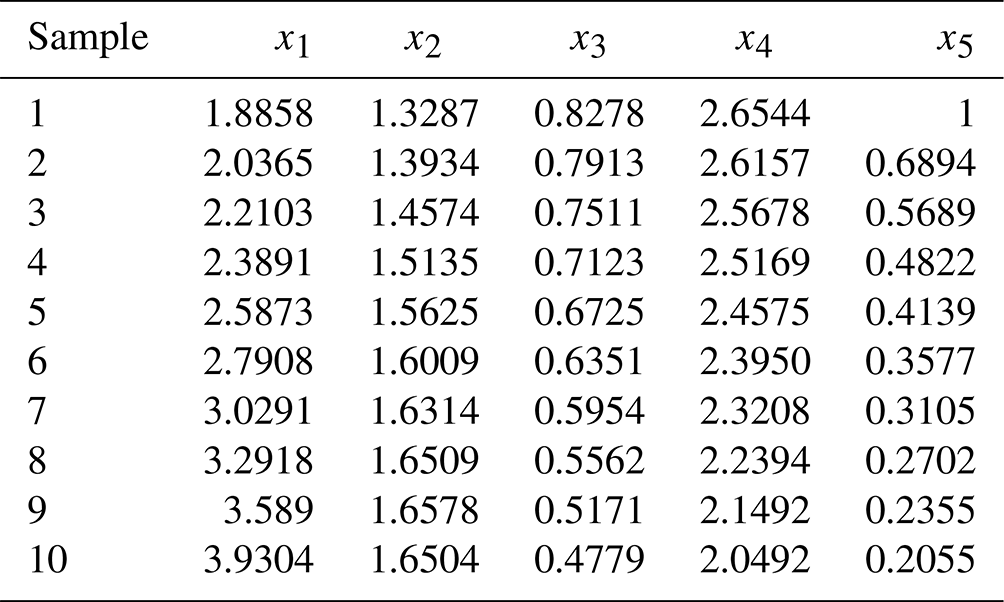
6.1 Interpolation point performance indicator data

As shown in Table 2, the robot arm tracking trajectory is interpolated into 10 interpolation points, each with its corresponding performance index.

Table 2 Performance index data of each interpolation point.

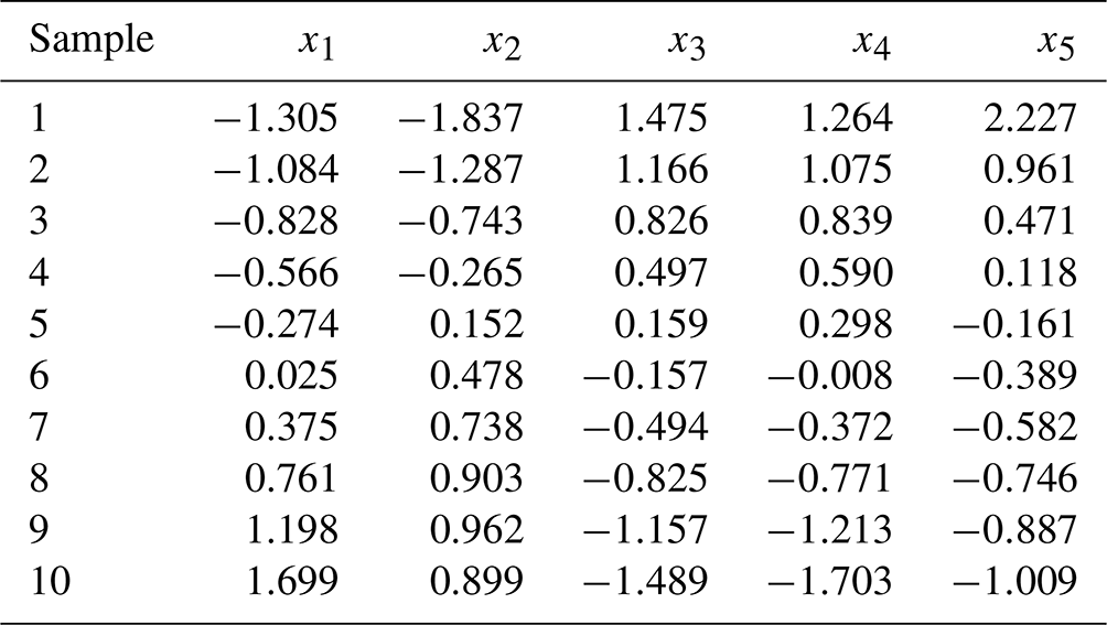
6.2 Data standardization

The four-sport flexibility indicators x₁, x₂, x₃, and x₄ and the reliability function data x₅ were normalized from the equations of the above principal component analysis method for the 10 interpolation points. See Table 3 for normalization results.

Table 3 Standardized performance index data of the manipulator.

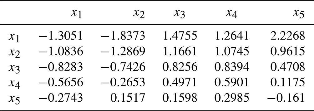
6.3 Calculating the correlation coefficient matrix R

From the above principal component analysis method equations, the correlation coefficient matrix R can be calculated for the four-sport flexibility indicators data (x₁, x₂, x₃, and x₄) and the reliability function data (x₅). See Table 4 for the results.

Table 4 Correlation coefficient matrix R of mechanical-arm performance indicators.

6.4 Determination of principal components

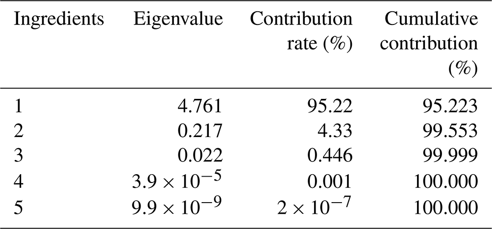
From Table 5, the cumulative variance contribution of the first principal component is 95.223 %, which is greater than 85 %, indicating that the first principal component responds to 95.223 % of the information we get from the original variable and basically reflects the information contained in all indicators. So the principal component is 1.

Table 5 Characteristic values, principal component contribution rate, and cumulative contribution rate.

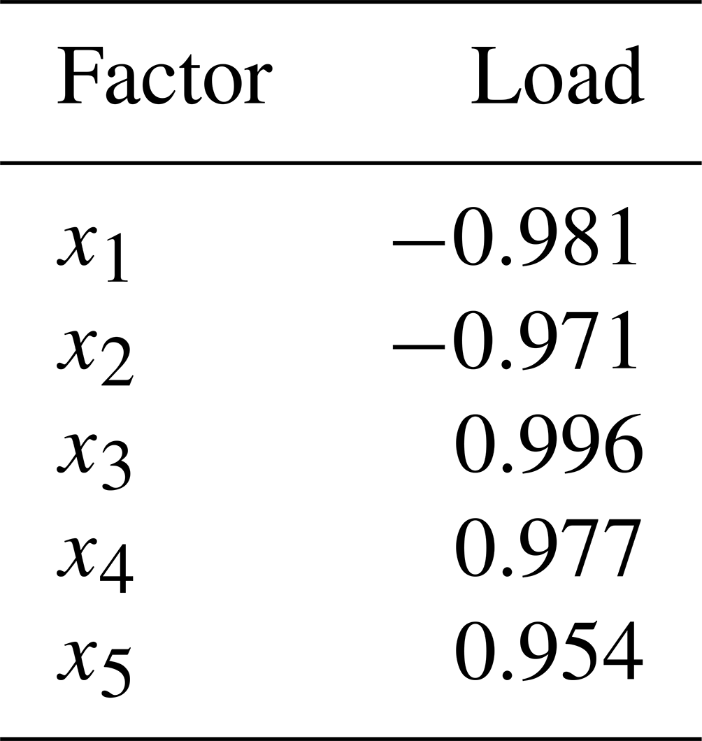
6.5 Determination of the integrated evaluation function

From the loadings of each indicator in Table 6, x₁, x₂, x₃, x₄, and x₅ all have high loadings on the first principal component. This means that the first principal component represents most of the five indicators' information. The original five variables can be replaced by one principal component variable. The first principal component represents a comprehensive evaluation indicator that combines the reliability function derived from the failure rate function of the prediction model and each indicator of the robotic arm.

Table 6 Factor load matrix.

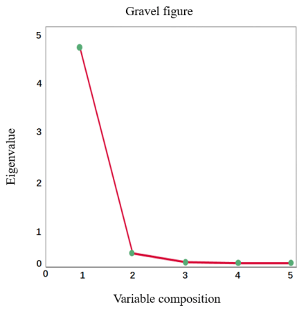
As can be seen from Fig. 1, the first principal component accounts for the largest proportion eigenvectors are obtained by dividing the data of the factor-loading matrix by the square root of its corresponding eigen root. Using the equation for principal component analysis, we multiply the resulting eigenvectors with the normalized data to obtain the principal component expression.

$$\begin{array}{}\text{(33)}& \begin{array}{rl}\mathbf{F}& =-\mathrm{0.4496}{x}_{\mathrm{1}}-\mathrm{0.4450}{x}_{\mathrm{2}}+\mathrm{0.4564}{x}_{\mathrm{3}}+\mathrm{0.4478}{x}_{\mathrm{4}}\\ & +\mathrm{0.4372}{x}_{\mathrm{5}}\end{array}\end{array}$$

This is a comprehensive evaluation function.

Figure 1 Gravel figure.

7 Sudden-speed-change suppression at the moment of failure based on coordinated resource allocation

In order to ensure that the end effector can complete its expected tasks after the mechanical arm fails, this paper uses the value of the integrated evaluation function as a criterion. According to the analysis, the larger the value, the better the performance and the smaller the impact on the overall performance when the fault occurs; conversely, the worse the performance, the greater the impact on the overall performance when the fault occurs.

The derivation is as follows: the Jacobi matrix is a linear transformation of the mapping of the joint space velocity $\dot{\mathbf{q}}$ to the operation space velocity $\dot{\mathbf{x}}$ (end velocity). The relationship between these two variables is

$$\begin{array}{}\text{(34)}& \dot{\mathbf{x}}=\mathbf{J}\dot{\mathbf{q}}.\end{array}$$

Define ${\dot{\mathbf{j}}}_k$ as the kth of the space of the robotic arm in terms of the Jacobi matrix J column.

$$\begin{array}{}\text{(35)}& \mathbf{J}=\left[{\dot{\mathbf{j}}}_{\mathrm{1}},\mathrm{\dots },{\dot{\mathbf{j}}}_{k-\mathrm{1}},{\dot{\mathbf{j}}}_k,{\dot{\mathbf{j}}}_{k+\mathrm{1}},\mathrm{\dots },{\dot{\mathbf{j}}}_n\right]\end{array}$$

Each column in the equation represents the contribution of the joint speed to the end speed.

The results are weighted on the basis of the optimal inverse-solution algorithm under fault-tolerant control in Sect. 4 to facilitate the allocation of individual rod speeds in the context of a coordinated resource allocation strategy. Namely,

$$\begin{array}{}\text{(36)}& {\mathbf{J}}^{+}={\mathbf{W}}^{-\mathrm{1}}{\mathbf{J}}^T{\left({\mathbf{JW}}^{-\mathrm{1}}{\mathbf{J}}^T\right)}^{-\mathrm{1}},\end{array}$$

where W is the diagonal matrix.

$$\begin{array}{}\text{(37)}& \mathrm{\text{diag}}\left(W\right)=\left[\begin{array}{cccccccc}{w}_{\mathrm{1}}& \mathrm{0}& \mathrm{0}& \mathrm{0}& \mathrm{0}& \mathrm{0}& \mathrm{0}& \mathrm{0}\\ \mathrm{0}& w_{\mathrm{2}}& \mathrm{0}& \mathrm{0}& \mathrm{0}& \mathrm{0}& \mathrm{0}& \mathrm{0}\\ \mathrm{0}& \mathrm{0}& \mathrm{\ddots }& \mathrm{0}& \mathrm{0}& \mathrm{0}& \mathrm{0}& \mathrm{0}\\ \mathrm{0}& \mathrm{0}& \mathrm{0}& w_{k-\mathrm{1}}& \mathrm{0}& \mathrm{0}& \mathrm{0}& \mathrm{0}\\ \mathrm{0}& \mathrm{0}& \mathrm{0}& \mathrm{0}& w_k& \mathrm{0}& \mathrm{0}& \mathrm{0}\\ \mathrm{0}& \mathrm{0}& \mathrm{0}& \mathrm{0}& \mathrm{0}& w_{k+\mathrm{1}}& \mathrm{0}& \mathrm{0}\\ \mathrm{0}& \mathrm{0}& \mathrm{0}& \mathrm{0}& \mathrm{0}& \mathrm{0}& \mathrm{\ddots }& \mathrm{0}\\ \mathrm{0}& \mathrm{0}& \mathrm{0}& \mathrm{0}& \mathrm{0}& \mathrm{0}& \mathrm{0}& w_n\end{array}\right]\end{array}$$

The resulting joint speed of the redundant robot can be expressed as follows:

$$\begin{array}{}\text{(38)}& \dot{\mathbf{q}}={\mathbf{J}}^{+}\dot{\mathbf{x}},\end{array}$$

where the full rank case (q)⁺ will satisfy the following condition so that the minimum parametric solution $(\mathbf{q}{)}^{+}\dot{\mathbf{x}}$ can also be obtained, and the solution is orthogonal to the zero space N(J).

$$\begin{array}{}\text{(39)}& \left\{\begin{array}{c}{\mathbf{JJ}}^{+}\mathbf{J}=\mathbf{J}\\ {\mathbf{J}}^{+}{\mathbf{JJ}}^{+}={\mathbf{J}}^{+}\\ {\left({\mathbf{J}}^{+}\mathbf{J}\right)}^T={\mathbf{J}}^{+}\mathbf{J}\\ \left({\mathbf{JJ}}^{+}\right)={\mathbf{JJ}}^{+}\end{array}\right.\end{array}$$

We expanded J⁺ to

$$\begin{array}{}\text{(40)}& {\mathbf{J}}^{+}=\left[\begin{array}{c}{J}_{\mathrm{1}}\cdot {\left(w_{\mathrm{1}}\cdot \mathit{\delta }\right)}^{-\mathrm{1}}\\ J_{\mathrm{2}}\cdot {\left(w_{\mathrm{2}}\cdot \mathit{\delta }\right)}^{-\mathrm{1}}\\ \mathrm{⋮}\\ J_{k-\mathrm{1}}\cdot {\left(w_{k-\mathrm{1}}\cdot \mathit{\delta }\right)}^{-\mathrm{1}}\\ J_k\cdot {\left(w_k\cdot \mathit{\delta }\right)}^{-\mathrm{1}}\\ J_{k+\mathrm{1}}\cdot {\left(w_{k+\mathrm{1}}\cdot \mathit{\delta }\right)}^{-\mathrm{1}}\\ \mathrm{⋮}\\ J_n\cdot {\left(w_n\cdot \mathit{\delta }\right)}^{-\mathrm{1}}\end{array},\right]\end{array}$$

where δ is

$$\begin{array}{}\text{(41)}& \mathit{\delta }=\sum _{i=\mathrm{1}}^n\left(J_i^{\mathrm{2}}\cdot w_i^{-\mathrm{1}}\right).\end{array}$$

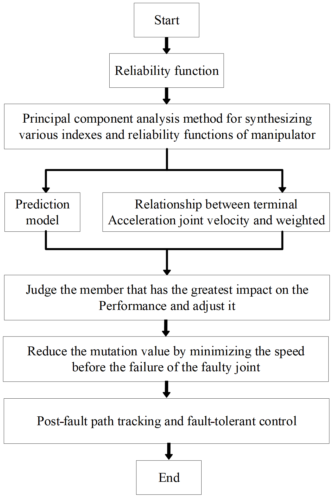
From the above equation, we can see that the elements J⁺ are closely related to the elements diag(W). If we want to reduce the speed of this joint, we need to increase the corresponding w_k to find the joint that has the greatest impact on the performance of the robot system after the failure and then adjust the joint. The larger the F value, the more reliable the w_k and the lower the speed suppression of the joint with the greatest impact on the performance of the robot system, and conversely, the larger w_k is, the higher the speed suppression of the joint with the greatest impact on the performance of the robot system. This principle is applied in combination with a comprehensive evaluation function to control the arm in order to reduce the probability of failure and to reduce the overall performance impact if a failure occurs. The algorithm has a certain universality.

The analysis process is shown in Fig. 2.

Figure 2 Flow chart of suppression algorithm based on fault prediction model.

8 Experimental validation

Joint performance in the event of failure without a coordinated resource allocation strategy

This paper validates the resource coordination allocation algorithm on a previously studied redundancy-degree robot object based on the concept of centralized drive arrangement. The model is shown in Fig. 3.

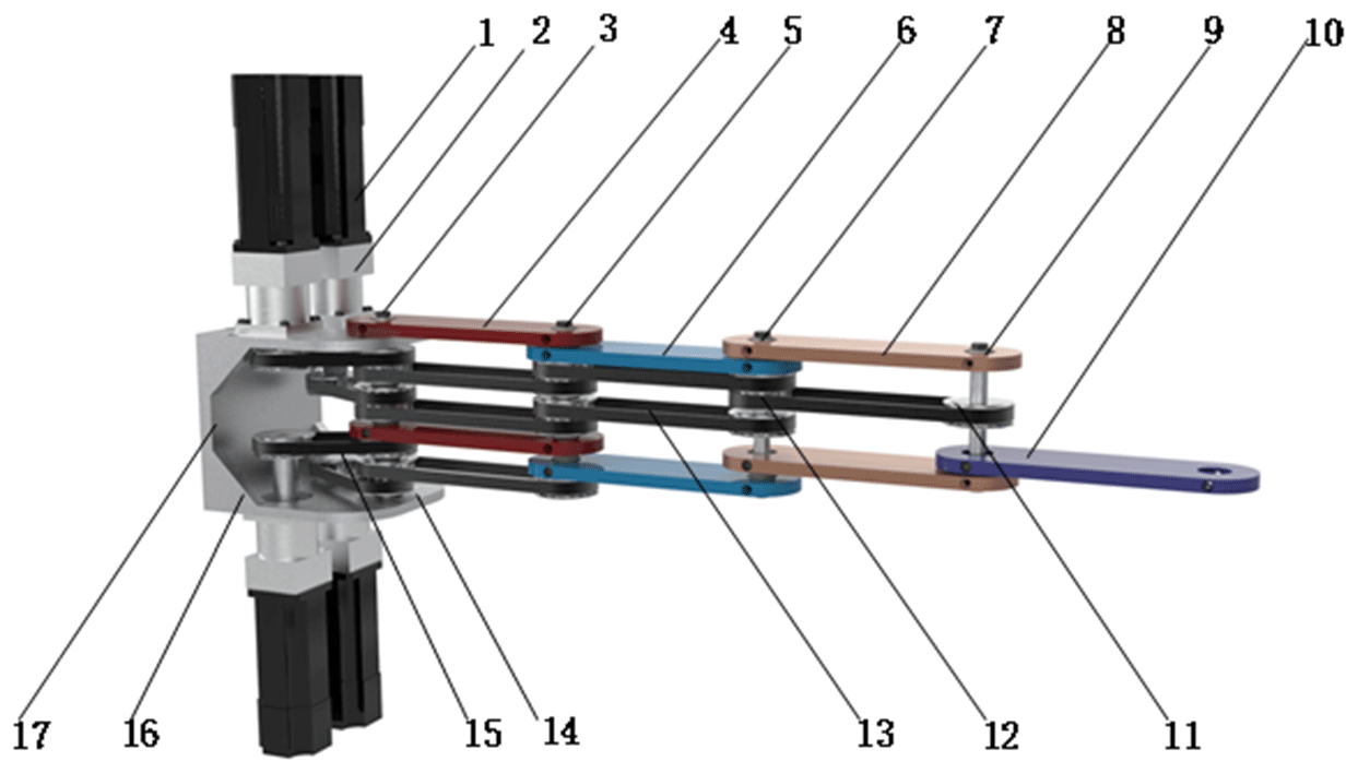
Figure 3 Three-dimensional diagram of 4R redundant robot: 1. servo motor, 2. planetary reducer, 3. axis I, 4. rod I, 5. axis II, 6. rod II, 7. axis III, 8. rod III, 9. axis IV, 10. rod IV, 11. small pulley, 12. large pulley, 13. long timing belt, 14. motor-connecting plate, 15. short timing belt, 16. stiffener, 17. wallboard.

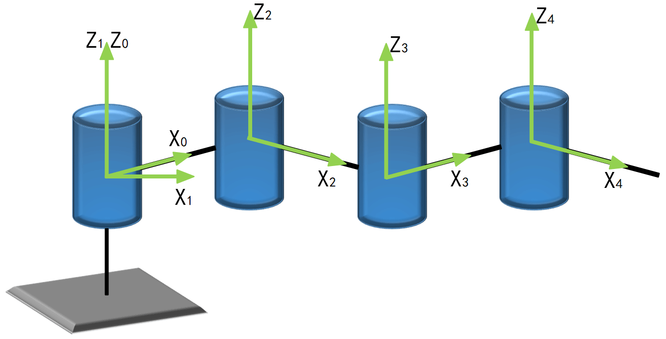
In the Cartesian coordinate system, each linkage is defined according to the D–H parameter method for the robot shown in Fig. 3, and the parameters of each linkage are set. The definition of each joint of the robot arm, as shown in Fig. 4, shows how the four links are connected in series and the rules for defining the coordinate system.

Figure 4 D–H coordinate system for planar 4R redundant robot.

The D–H parameters for the planar 4R redundant robot are shown in Table 7.

Table 7 D–H link parameters of 4R redundant robot.

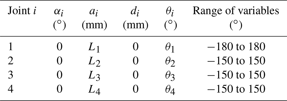
α_i: connecting-rod turning angles; a_i: connecting-rod length; d_i: connecting-rod deflection distance; θ_i: joint angle.

In this paper, the main research of joint failure after the stuck fault forms. The optimal algorithm in Sect. 7 is used to control the arm, tracking a straight line, assuming that the fault is accurately detected and that the fault occurs in 5 s. The simulation results are shown below.

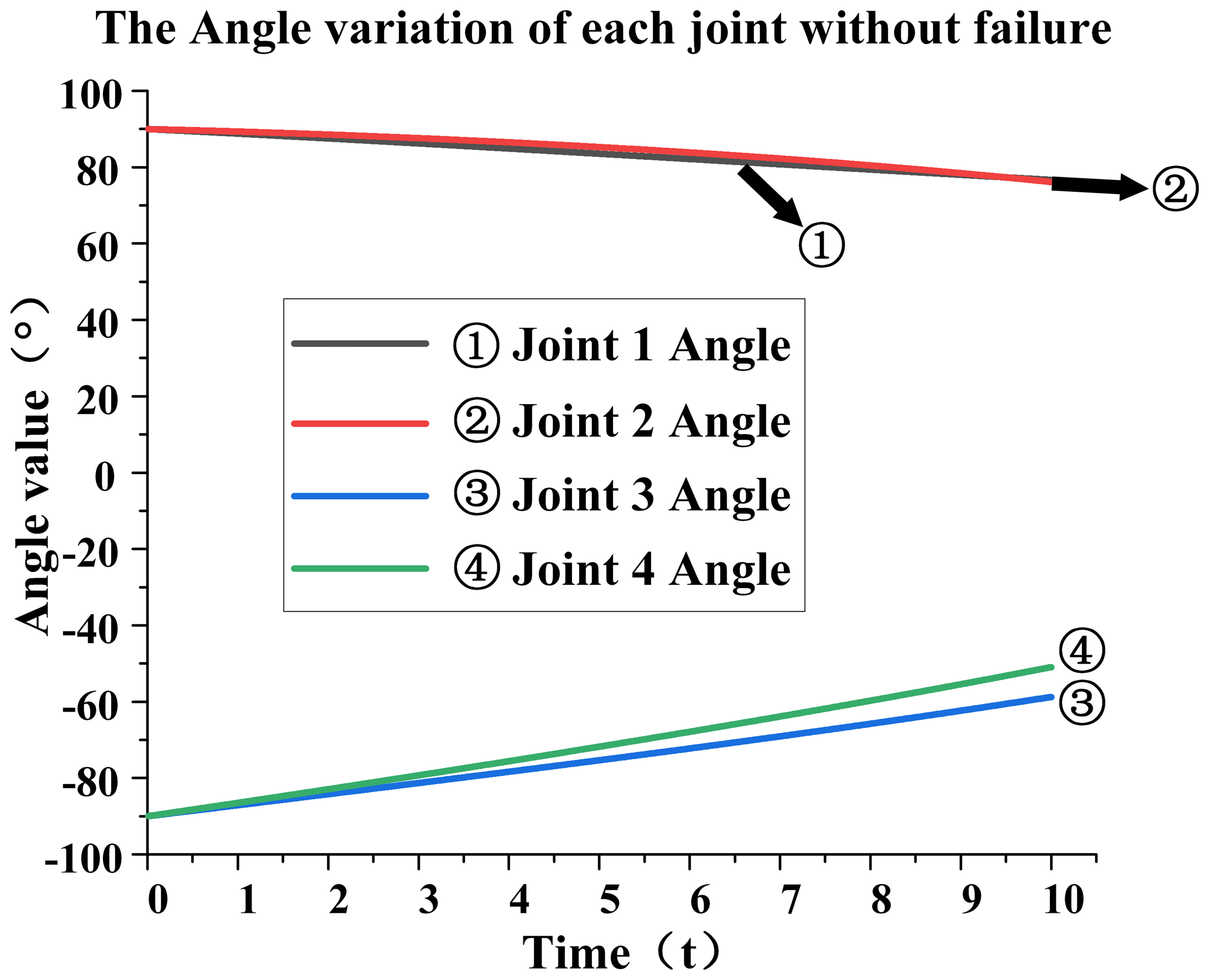
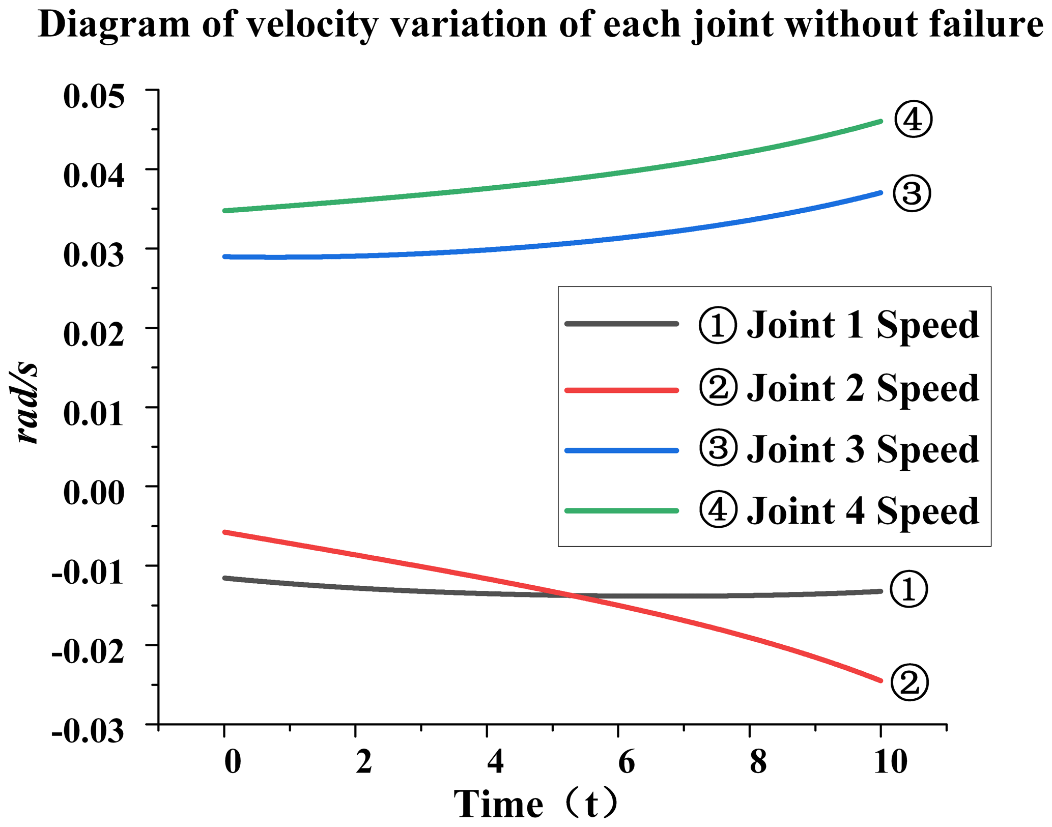
No failures. It can be seen from Figs. 5 and 6 that, when the joint is in a healthy state, the angle change and velocity of each joint are relatively stable without mutation, and these data can be used as the control data.

Figure 5 Diagram of joint angle changes without failure.

Figure 6 Diagram of joint velocity variation without failure.

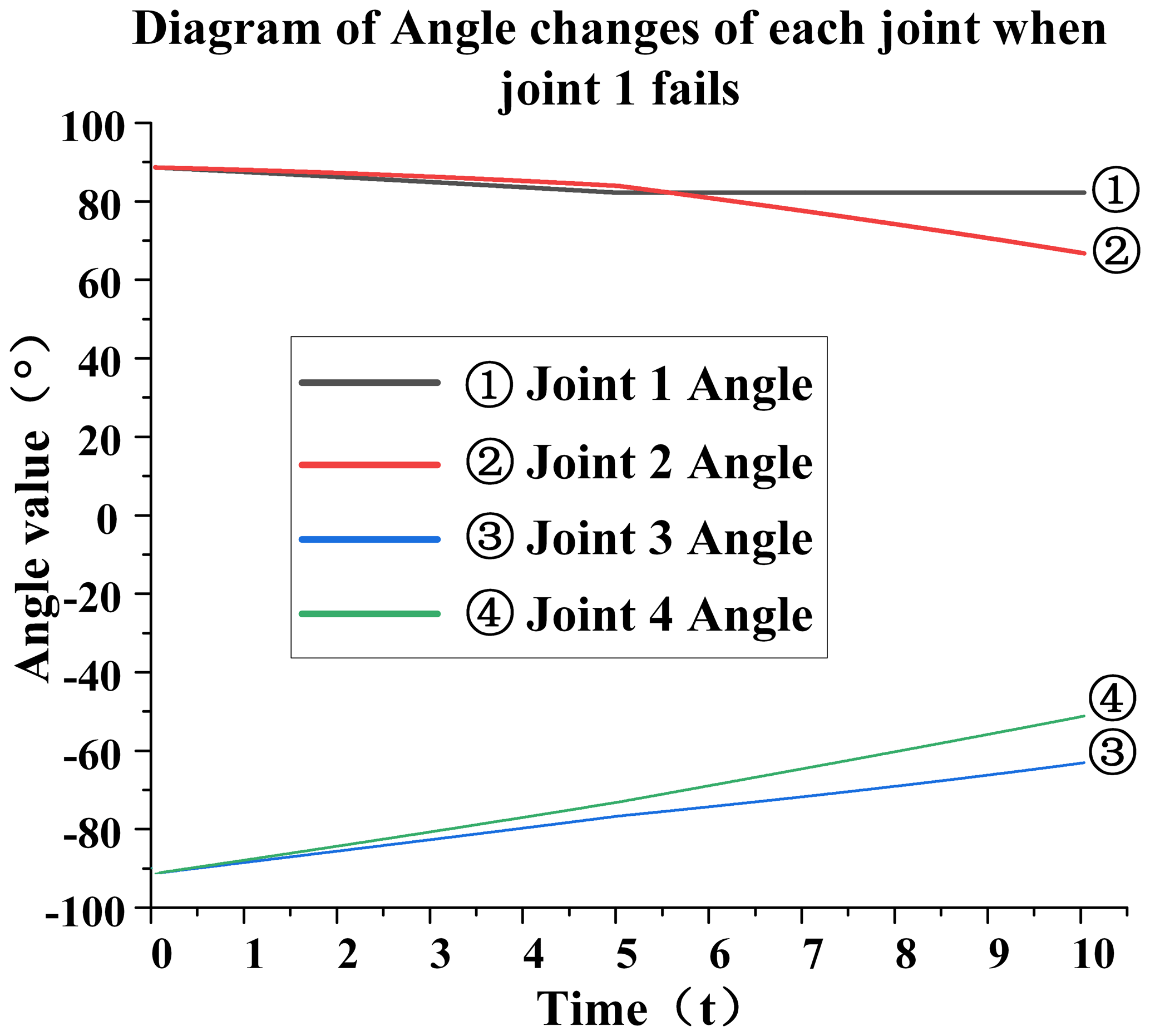
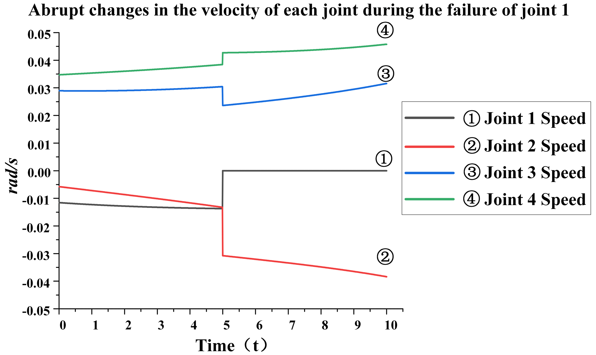
Failure of joint 1. When joint 1 fails, the specific analysis is as follows: from Fig. 7, it can be seen that, at the fifth second, joint 1 will remain at 83^∘ and will not change. This is because the joint is stuck after the failure at this moment, resulting in the angle of joint 1 not changing. It can be seen from Fig. 8 that, at the fifth second, the speed of each joint has a sudden-change value. The speed of joint 1 directly changes from −0.012 to 0 rad s⁻¹, and the sudden-change value is 0.012; the speed of joint 2 changes from −0.011 to −0.03 rad s⁻¹, and the sudden-change value is 0.019; the speed of joint 3 changes from 0.031 to 0.024 rad s⁻¹.

Figure 7 Diagram of angle changes of each joint when joint 1 fails.

Figure 8 Abrupt changes in the velocity of each joint during the failure of joint 1.

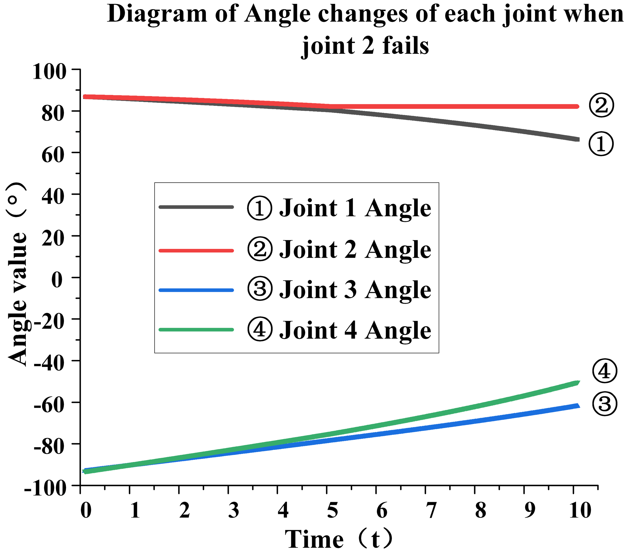
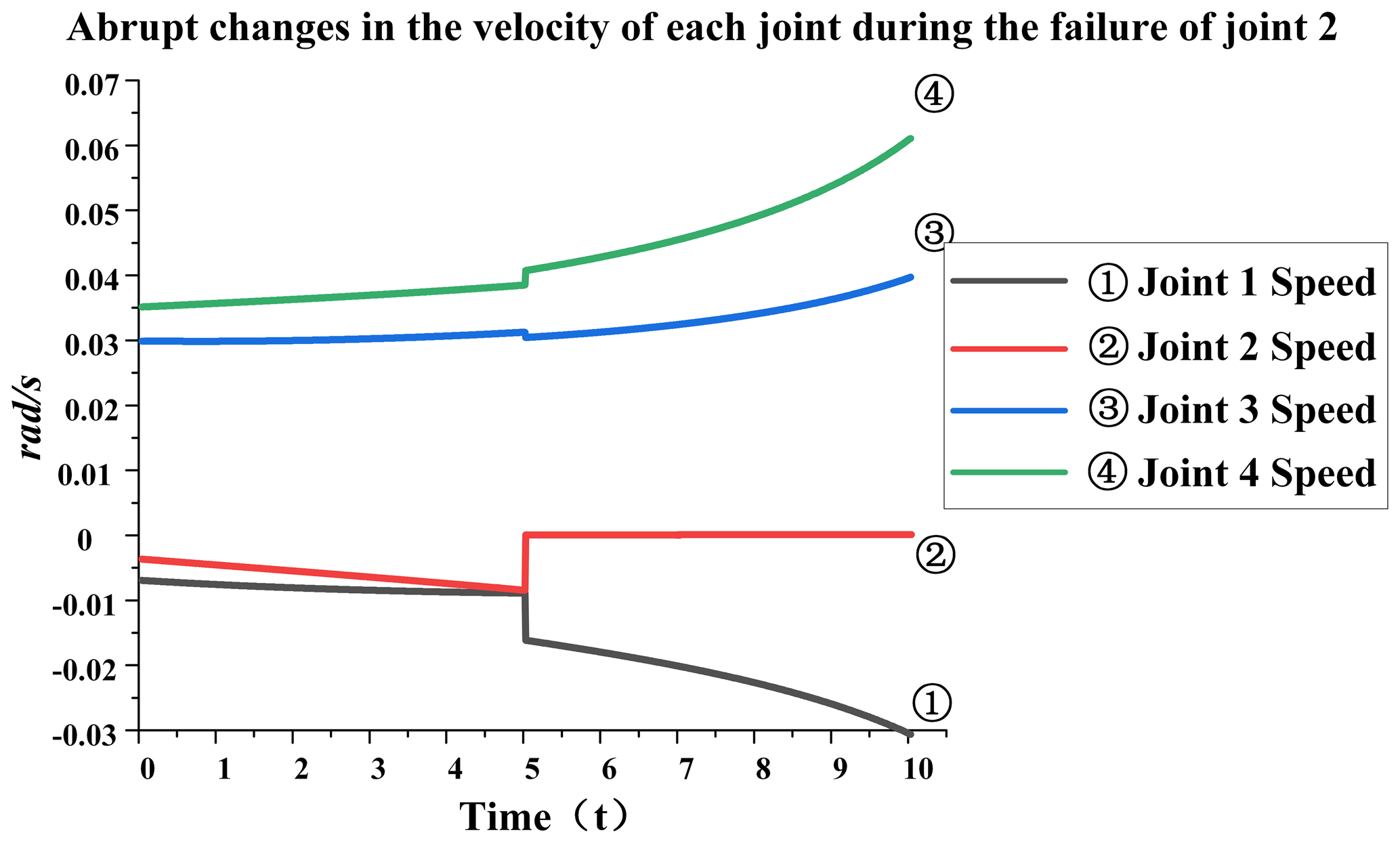
Failure of joint 2. When joint 2 fails, the specific analysis is as follows: from Fig. 9, it can be seen that, at the fifth second, joint 2 will remain at 82^∘ and will not change because the joint is stuck after the failure at this moment, resulting in the angle of joint 2 not changing. It can be seen from Fig. 10 that, at the fifth second, the speed of each joint has a sudden-change value. The speed of joint 1 has changed from −0.008 to −0.016 rad s⁻¹, and the sudden-change value is 0.008; the speed of joint 2 has changed from −0.007 to 0 rad s⁻¹, and the sudden-change value is 0.007; the speed of joint 3 has changed from 0.032 to 0.031 rad s⁻¹, and the sudden-change value is 0.001; the speed of joint 4 has changed from 0.039 to 0.041 rad s⁻¹, and the sudden-change value is 0.002. The total sudden-change variable is 0.018, which can be seen from the data. When joint 2 fails, the overall sudden change is not very large, but relatively speaking, it has a greater impact on joint 1 than on other joints.

Figure 9 Diagram of angle changes of each joint when joint 2 fails.

Figure 10 Abrupt changes in the velocity of each joint during the failure of joint 2.

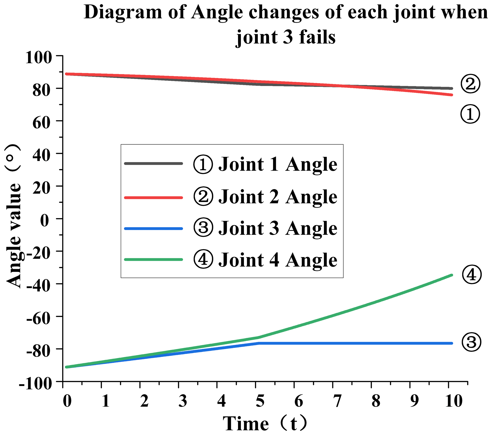
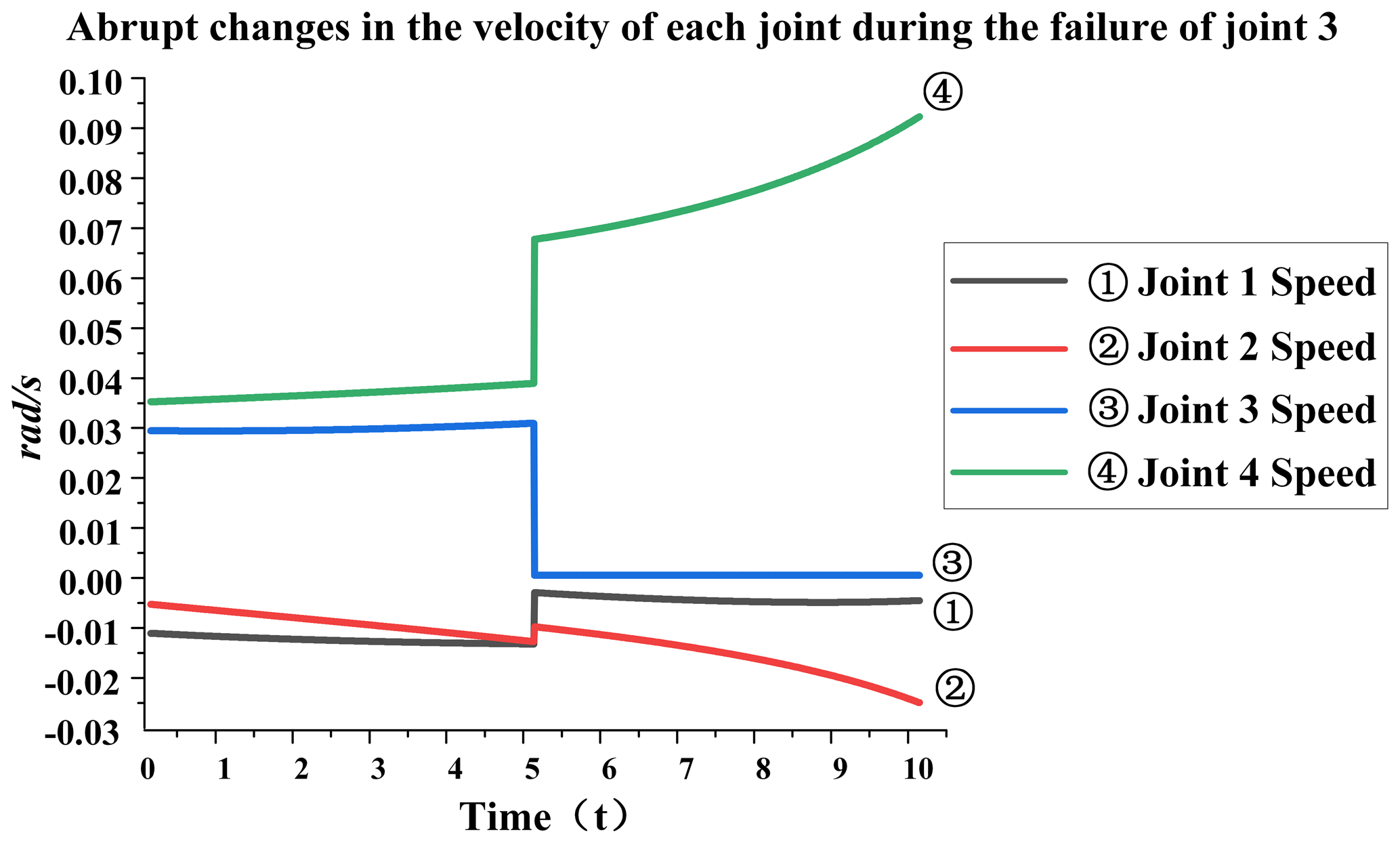
Failure of joint 3. When joint 3 fails, the specific analysis is as follows: from Fig. 11, it can be seen that, at the fifth second, joint 3 will remain at −79^∘ and will not change. This is because the joint is stuck after the failure at this moment, resulting in the angle of joint 3 not changing. Joint 4's final angle changes greatly. When no failure occurs, the angle is −52^∘, and the current angle is −38^∘. It can be seen from Fig. 12 that, at the fifth second, the speed of each joint has a sudden-change value. The speed of joint 1 has changed from −0.011 to −0.001 rad s⁻¹, and the sudden-change value is 0.01; the speed of joint 2 has changed from −0.011 to −0.008 rad s⁻¹, and the sudden-change value is 0.003; the speed of joint 3 has changed from 0.031 to 0 rad s⁻¹, and the sudden-change value is 0.031; the speed of joint 4 has changed from 0.039 to 0.068 rad s⁻¹, and the sudden change value is 0.029. The total sudden-change value is 0.073, which can be seen from the data. When joint 3 fails, the overall sudden variable is relatively large, and the impact on joint 4 is greater than that on other joints.

Figure 11 Diagram of angle changes of joints when joint 3 fails.

Figure 12 Abrupt changes in the velocity of each joint during the failure of joint 3.

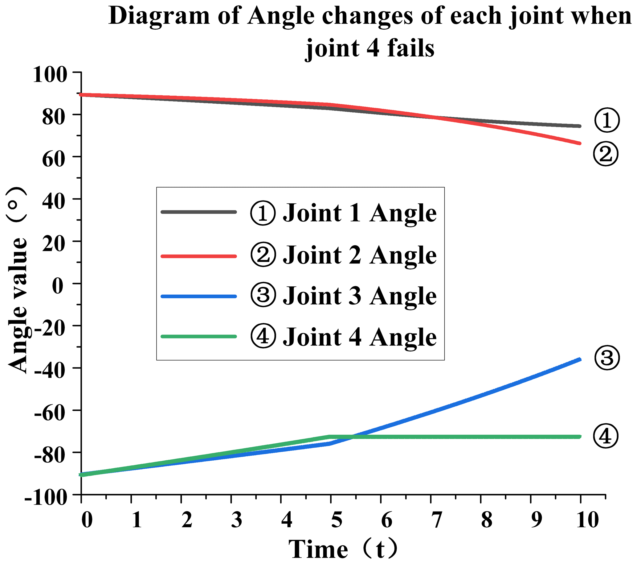
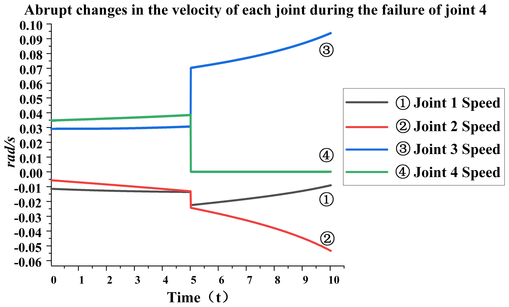
Failure of joint 4. When joint 4 fails, the specific analysis is as follows: from Fig. 13, it can be seen that, at the fifth second, joint 4 will remain at −76^∘ and will not change. This is because the joint is stuck after the failure at this moment, resulting in the angle of joint 4 not changing anymore. The rearmost angle of joints 2 and 3 will change, but joint 3 will change a little more. It can be seen from Fig. 14 that, at the fifth second, the speed of each joint has a sudden-change value. The speed of joint 1 changes from −0.011 to −0.023 rad s⁻¹, and the sudden-change value is 0.012; the speed of joint 2 changes from −0.011 to −0.023 rad s⁻¹, and the sudden-change value is 0.012; the speed of joint 3 changes from 0.032 to 0.072 rad s⁻¹, and the sudden-change value is 0.06; joint 4 changes from 0.039 to 0 rad s⁻¹, and the sudden change value is 0.029. The total sudden-change value is 0.113, which can be seen from the data. When joint 4 fails, the overall sudden variable is relatively large, and the impact on joint 3 is greater than that on other joints.

Figure 13 Diagram of angle changes of joints when joint 4 fails.

Figure 14 Abrupt changes in the velocity of each joint during the failure of joint 4.

The data from the moment before and the moment after the moment of failure were calculated to collate the data in Table 8.

Table 8 Index data affecting the performance of different joint failures.

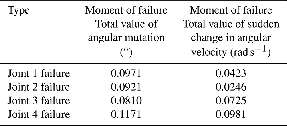
The analysis in Table 8 shows that the overall performance is most affected by a failure in joint 4; thus, the resource coordination allocation algorithm is controlled for joint 4.

9 Adopting a coordinated resource allocation strategy for joint performance in case of failure

From Sect. 8.1, it is clear that a failure of joint 4 has the greatest impact on overall performance; thus, the method in Sect. 6 is used to control joint 4. The graph below shows the change in speed and angle of each joint following a failure of joint four after control using the coordinated resource allocation strategy.

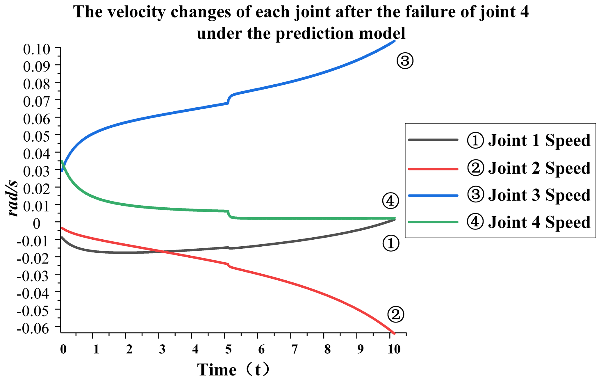
Figure 15 The velocity changes of each joint after the failure of joint 4 under the prediction model.

Figure 16 The angle changes of each joint when joint 4 fails under the prediction model.

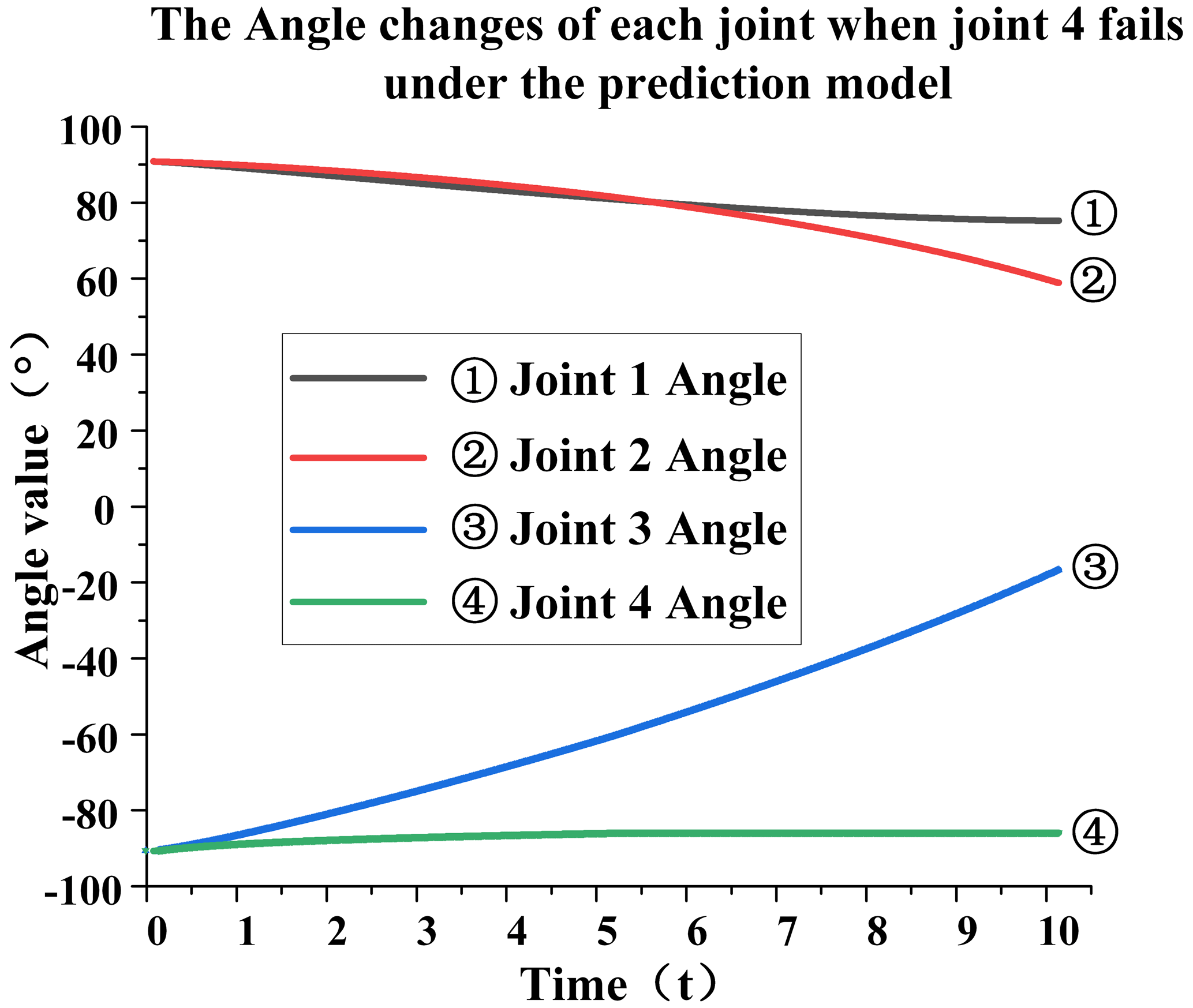
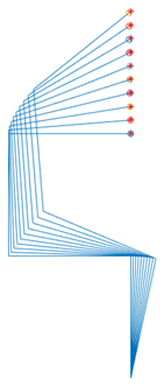
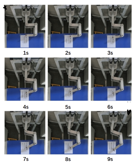
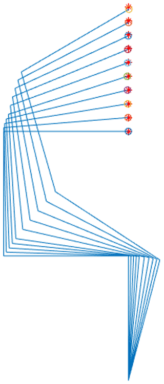
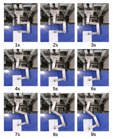
According to Fig. 15, it can be seen that the velocity of joint 4 had reduced to approximately near zero before the 5 s failure moment occurred. As can be seen from Fig 16, the angular fluctuation is negligible; thus, the sudden change in joint velocity after the failure occurred was minimal and had very little effect on the robot trajectory tracking. It can be seen that there is almost no mutation in joint 1 at the time of failure. The mutation value of joint 2 is 0.003, that of joint 3 is 0.005, that of joint 4 is 0.004, and the total mutation value is 0.012, which greatly reduces the impact of joint failure on the overall performance. Figures 18 and 20 show the physical verification images of the tracking-line trajectory. The morphology diagram shows that the attitude of the fourth joint was mediated before the failure occurred, as can be seen in the completely different attitude of the tracking-line simulation diagrams in Figs. 17 and 19.

Figure 17 End tracking-status diagram without failure.

Figure 18 State diagram of redundant robot after 1–9 s each time a fault occurs.

Figure 19 Terminal tracking-trajectory-state diagram when joint 4 fails.

Figure 20 State diagram of redundant robot after 1–9 s each time joint 4 fails.

Since our main concern is the fault-tolerant control strategy after the fault occurs, which is to ensure the minimum instantaneous impact of the equipment failure and to ensure the stability of the job processing, we assume that the mode failure will occur at a certain time so we did not predict the fault in advance in the study. We will study robot failure prediction in future research work.

10 Conclusions

The main innovation of this paper is to integrate the bathtub hazard rate curve with various performance indicators of the robot; to propose the obtainment of the comprehensive evaluation function through the principal component analysis method; and to take the function as the mathematical model of resource coordination allocation strategy, to take the planar redundant robot as the research object based on the inverse kinematics of the fault-tolerant control of the optimal redundancy, and to realize the adjustment of the rod that has the greatest impact on the performance after failure. This reduces the probability of failure and the impact on the overall performance after a fault occurs. Through the above theoretical derivation and verification of simulation results and experimental results, the following conclusions can be drawn:

• 1.

  The sudden change in angle after the failure of each joint shows that the sudden change in the speed of the joints close to the failed joint is greater than that of the joints far from the failed joint; i.e., the performance of the joints close to the failed joint is more affected after a failure.

• 2.

  It can be seen from the simulation verification in Figs. 17 and 19 and the physical verification in Figs. 18 and 20 that the fault-tolerant control method based on coordinated resource allocation can ensure that the end trajectory coincides with the target trajectory after a failure.

• 3.

  A comparison of Figs. 14 and 15 shows that the fault-tolerant control method based on coordinated resource allocation can effectively reduce the impact on the overall performance after a failure.

• 4.

  A synthesis of the figures in the text shows that the fault-tolerant control method based on the coordinated allocation of resources can ensure that the sudden change in joint speed is greatly reduced without a sudden change in end speed at the moment of failure.

This method can reduce the impact on the overall performance of the robot after joint failure to a certain extent, but there are still a few mutations in the final result. Therefore, more appropriate fault prediction functions and more feedback data are needed to further optimize the coordinated allocation of resources among the robot joints.