the Creative Commons Attribution 4.0 License.
the Creative Commons Attribution 4.0 License.
 | 25 Jul 2023
Robust trajectory tracking control for collaborative robots based on learning feedback gain self-adjustment
Xiaoxiao Liu
Mengyuan Chen
A robust position control algorithm with learning feedback gain automatic adjustment for collaborative robots under uncertainty is proposed, aiming to compensate for the disturbance effects of the system. First, inside the proportional-derivative (PD) control framework, the robust controller is designed based on model and error. All of the model's uncertainties are represented by functions with upper bounds in order to surmount the uncertainties induced by parameter changes and unmodeled dynamics. Secondly, the feedback gain is automatically adjusted by learning, so that the control feedback gain is automatically adjusted iteratively to optimize the desired performance of the system. Thirdly, the Lyapunov minimax method is used to demonstrate that the proposed controller is both uniformly bounded and uniformly ultimately bounded. The simulations and experimental results of the robot experimental platform demonstrate that the proposed control achieves outstanding performance in both transient and steady-state tracking. Also, the proposed control has a simple structure with few parameters requiring adjustment, and no manual setting is required during parameter setting. Moreover, the robustness and efficacy of the robot's trajectory tracking with uncertainty are significantly enhanced.
- Article
(8661 KB) - Full-text XML
- BibTeX
- EndNote


Collaborative robot (CoBot) is a kind of robot with high flexibility, security, and cooperation, which can work in the same workspace as human beings and complete tasks together (Lytridis et al., 2021; Fan et al., 2023; Zhai et al., 2022). Compared with traditional industrial robots, collaborative robots are adaptive and customizable, which can quickly adapt to diverse production and service needs, and well meet the requirements of flexible customization in intelligent manufacturing. Collaborative robots have higher safety, enabling robots to completely eliminate the constraints of fences or cages while eliminating barriers to human–robot collaboration. Its pioneering product performance and wide range of application areas have opened up a new era for the development of robots. With aging and the increase of labor costs, reducing labor and reducing human labor intensity has become a major consideration for all walks of life and even families, and it provides a great application space for collaborative robots. For example, in the modern logistics industry, the use of collaborative robots has become a trend due to the significant increase in the type, quantity, and sorting speed of goods. In the medical industry, surgical robots have become a successful model of collaborative robots. Collaborative robots will play an important role in the fields of housekeeping and elderly care services; in nuclear power, aerospace, and other special environmental fields, collaborative robots have also shown good application prospects, and more applications are also being planned.
With the increasing demand for high speed, high precision, and high compliance of collaborative robots, their dynamic modeling and control must be paid attention to. Nevertheless, the collaborative robot system is a complex nonlinear system with time-varying, multiple-input, and multiple-output coupling. When the robot is in a state of continuous motion, its nonlinear dynamic control is of the utmost importance, and it is essential to optimize the design of trajectory tracking controllers so that the robot arm can perform trajectory tracking tasks more effectively. Academic researchers have made considerable efforts to enhance the performance of collaborative robots' trajectory tracking, such as computing torque control (Ghediri et al., 2022; Ramuzat et al., 2022), disturbance observer (Jie et al., 2020; Regmi et al., 2022; Salman et al., 2023), adaptive immunity control (ADRC; Khaled et al., 2020; Ma et al., 2021; Guo et al., 2016; Gaidhane et al., 2023), fuzzy control (Xian et al., 2023; Jiang et al., 2020), and sliding mode control (SMC; Lv, 2020; Duan et al., 2022; Zhao et al., 2022). These control algorithms can greatly improve the trajectory tracking performance of the robot to some extent, but they also have some shortcomings, for example, computational torque control and optimal control cannot handle uncertainties such as parameters, external disturbances, and variable loads well. The disturbance observer-based compensation control can impose more precise control, but this method is extremely demanding on the model and typically requires a great deal of time for identification. Adaptive control realizes the adaptive update of controller parameters through the online identification of parameters, but the control performance depends on the parameter identification accuracy, and the transient response performance is not good (Guo et al., 2017). Sliding mode variable structure control has good anti-interference performance after the system reaches the sliding mode surface, but it has a shortage of chattering.
Due to the complex characteristics of the robot system, there are always parameter uncertainties and external disturbances in practical applications. Because it does not require an excessive amount of model information, proportional-integral-derivative (PID) control has become the most common and standard technique. For application occasions with general trajectory accuracy requirements, small load, and low speed, PID control may meet the requirements, but for occasions with complex trajectories, high speed, and high accuracy requirements, it is difficult for traditional PID control to meet the requirements. Therefore, by combining the PID algorithm with other algorithms, some new algorithms have also emerged, such as the fuzzy control algorithm (Li et al., 2022), synovial control algorithm (Zhang, 2016), and neural network control algorithm (Xu and Wang, 2023). For instance, in Muñoz-Vázquez et al. (2019), a control scheme based on fuzzy control was proposed to synthesize PID error manifolds to improve the tracking ability of closed-loop systems. In Zhong et al. (2021), a fuzzy adaptive PID fast terminal sliding mode controller for redundant manipulator systems with variable loads is proposed. This controller can accomplish accurate monitoring of the manipulator's end effector trajectory. In Xiao et al. (2022), for instance, an adaptive proportional-integral-derivative (PID) controller based on a radial basis function (RBF) neural network is utilized to enhance the manipulator's tracking performance. The RBF neural network modifies its parameters based on the difference between the network output and the system output. The PID parameters are modified using the Jacobian matrix and motion error. But these algorithms are essentially PID algorithms, increasing the algorithm's complexity. In order to improve the overall performance of collaborative robots, we have also built more advanced control methods based on PID, such as dynamic feedforward control (Niu et al., 2019; Zaiwu et al., 2021) and adaptive robust control (ARC; Yin and Pan, 2018; Kong et al., 2020). These control methods are established for complete dynamic models and have shown good results. For example, Zhang et al. (2022) closed a study gap by suggesting feedforward recoil and static friction correction and by focusing on reducing mistakes during joint inversion. The results of the experiments show that the feedforward compensation makes the robot much more accurate when the joints are inverted, cutting the error by more than 70 %. In Ryu et al. (2000) a new method for making a robust controller was suggested to obtain a less conservative feedback controller. This method was used to make a single-link flexible manipulator. The goal is to obtain the best control performance when there are big weights that change over time. This will make sure that the flexible manipulator is stable when the tip position is changed. A robust control was proposed by Zhen et al. (2000). Using the upper limit of parameter uncertainty to improve the robot's dynamic performance can give good control performance to deal with system problems caused by parameter changes. There are many methods that are similar, but setting and adjusting the settings in these methods is hard and complicated. Also, these controllers do not take into account the dynamic properties, coupling relationships, and control needs of complex nonlinear robot systems. They cannot handle changes and doubts in the system well. Robots work in complicated environments with many unknowns, especially when they are used in real engineering. Our new goal is to make a controller that makes sure the output tracking error of the uncertainty model is always within a certain range and also lets key parameters be changed automatically online.
Therefore, combined with the problems existing in practical engineering, a simple and feasible robust trajectory tracking control algorithm for collaborative robots based on learning feedback gain self-adjustment is proposed in this paper. Firstly, the control of the collaborative robot is first divided into a nominal part and an uncertainty part. The parameters of the nominal parts are measured according to the robot manufacturer or the CAD software. However, all uncertainties of dynamic models are represented by corresponding functions, and the upper bound is assumed to be expressed in scalar form, which overcomes the uncertainties caused by parameter variations and unmodeled dynamics. Then, in the proportional-derivative (PD) control framework, a powerful controller is created based on the model and errors, and the feedback gain is automatically adjusted by learning. This allows the control feedback gain to be altered automatically repeatedly to achieve the highest possible level of system performance. Finally, the Lyapunov minimax approach is used to demonstrate that the recommended controller satisfies both uniform boundedness and uniform ultimate boundedness. This conclusion was reached by demonstrating that the suggested controller satisfies both of these conditions. This shows that the system is stable. Compared with existing robust control methods such as model predictive control (MPC), SMC, and ADRC, the proposed control method has a simple structure, and fewer parameters to be adjusted, and the parameter tuning process does not need to be manually set, which can be completed by learning, and the robustness is also good.
In particular, this paper's main contributions can be described as follows.
- 1.
Taking into account real-world engineering applications, a PD-based stable controller is created and applied to a nonlinear joint module system with uncertainty. It inherits the traditional PD control and robust control. With error-based and model-based features, accurate position tracking can be achieved.
- 2.
The control feedback gain is automatically adjusted by learning so that the desired performance of the system is optimized by iteratively adjusting the control feedback gain automatically. The dynamic model after feedback has a simple structure, self-adjusting parameters, and good robustness, which is practical in engineering.
- 3.
Numerical simulations and experimental verification are carried out on a two degrees-of-freedom (2-DOF) collaborative platform. Experiments that track harmonic signals and step signals are used to compare how well the three control methods work. Simulations and experiments show that the suggested control method can do a better job of following a route than other control methods.
The rest of this article is organized as follows. The first section describes the relevant literature review. The second section describes the dynamics model of the robot trajectory tracking and the controller design process. The third section gives the corresponding proof. The fourth section describes the experimental work and the obtained results. Finally, the conclusions are given to summarize the research work in this paper.
2.1 System modeling
The dynamics of a rigid linkage robot arm have been modeled in the literature on robotics:
where stands for the two angles at the joint and stands for the two torques at the joint. Assume that the inertia matrix H is nonsingular and given by the following equation:
where
where l1 and l2 represent the lengths of the first and second linkages, lc1 and lc2 represent the distance between the first and second links and joints 1 and 2, m1 and m2 represent the masses of the first and second linkages, and I1 and I2 represent the inertia matrices of the first and second linkages, respectively.
The following formula describes the matrix of centrifugal forces and force coefficients:
The gravity vector is defined as follows:
where g is the gravitational constant of the Earth.
The following is the formula for the damping matrix D.
The first and second joints have damping coefficients ς1 and ς2, respectively.
Consider the following uncertainties in the practical use of Model (1):
where the bounded uncertainty of the damping matrix , , is an uncertainty unknown perturbation with .
In this case, we consider Model (6) as an affine uncertain nonlinear system with the following structure:
where x∈ℝn is the state, u∈ℝm is the control input, y∈ℝp is the controlled output, x0 is the given finite initial condition, Δf denotes an unknown matrix or vector with uncertainty in the model. The column and function h of the vector field f, Δf, g satisfy the following assumptions.
Hypothesis 1: the columns of and are vector fields C∞ on a bounded set , which is the function of C∞ on X, and the vector fields Δf(⋅) is the function of C1 on X.
Hypothesis 2: Model (6) has a well-defined order at each point x0∈X, that is , and the system can be linearized in the following form: .
Hypothesis 3: the indeterminate vector function Δf(⋅) meets the condition , where Ψ(x) is a continuous function that is not negative.
Taking into consideration Hypothesis 2 and the nominal requirements, which are Δf=0, System (7) may be expressed as follows:
where , and b, A is the function of g, f, and h; there is no single form of A on X.
When the nominal Model (8) is taken into consideration, we are able to create a virtual input vector ν. Let
Then virtual linear input–output mapping can be obtained as follows:
Correspondingly, the stabilization output feedback of the system at this time is
If the tracking error is set as , then the tracking error of the system is
By adjusting the gain so that the polynomials in Eq. (12) are all Hurwitz. It is possible to derive the global asymptotic convergence of the tracking error, denoted by ϕi.
Our goal is to design a controller with feedback to ensure that the output tracking error of the uncertain model is consistently bounded and that the calming feedback gain K can be automatically adjusted online iteratively, where the automatic adjustment is used for performance optimization. The following actions help control the model: first, you need to create the robust controller to make sure that the tracking error is confined dynamically. It is then combined with a model-free learning algorithm to autonomously and iteratively modify the controller's feedback gain.
2.2 Robust controller design
Consider the case of a robotic arm system for the control of trajectory tracking. Assume that the intended angle of the trajectory is Θd, angular velocity is , and angular acceleration is ; Θd is continuously second-order derivable at [t0,∞], and they are consistently bounded.
Let
Then and . We rewrite the dynamics model (6) in the form of Eq. (8), where and . Based on the modeling analysis in the previous section, we can then write the following robust controller containing output feedback νs:
According to Eq. (11) we can obtain
where , . Kp is the proportional control parameter and Kd is the differential control parameter. These control parameters are derived from conventional PID control. Both the proportional and differential control parameters are denoted by the letters Kp and Kd, respectively. The traditional PID control served as the basis for deriving these control parameters.
In fact, due to the variation of the values in the model and the unmodeled part of the dynamics, as well as the uncertainties in the system, it is impossible to obtain the exact model characteristic matrix. Consequently, the array of dynamical model eigenvalues can be separated into a nominal portion and an uncertain portion.
where , , , and are the deterministic term of the corresponding matrix/vector, while the nominal part contains the uncertainty ΔH(⋅), ΔC(⋅), ΔG(⋅) and ϖD(⋅) depends on σ, which is an uncertain parameter in the robotic arm system and is time varying.
The dynamics model controller satisfying Eq. (14) also has the following fundamental properties.
Property 1: for a robotic system where is a symmetric positive definite bounded matrix, there exist scalar constants , for all such that
I is the identity matrix, and and are scalars that can be determined.
Property 2: the matrix is a skew-symmetric matrix, is the derivative of with respect to time, and for any γ∈Rn there exists
For a given , si>0, assume that the boundary of model uncertainty is scalar d and put all uncertainties into the function Ξ; then the relationship is as follows:
in the formula
The problem to be solved so far is to design a control law to ensure that the tracking error is within a predefined bound. We define the nominal systematic error as follows:
The controller design should also make ϕ(t) asymptotic stability; the designed controller is
The controller is based on the nominal system tracking error ϕ(t) and system uncertainty, the first six terms are used only to indicate the nominal system (i.e., a system without uncertainty), and the last term compensates for system uncertainty, where κ is an adjustable constant variable and κ>0.
2.3 Automatic adjustment of learning-based feedback gain
Despite the model uncertainty of the system, our task is to track the desired output trajectory, and there are feedback gains kd1, kd2, kp1, and kp2. Manually adjusting the gains requires additional time. In this setting, a gain that can be automatically altered while maintaining system stability during adjustment is crucial and is referred to in the industry as the auto setting.
Therefore, we must initially define an appropriate learning cost function that characterizes the intended controller performance. Since the ultimate control goal is output trajectory tracking, choose the following tracking cost function:
where signifies the amount of repetitions, tf is the length of the finite interval in which each iteration occurs, , , and . α is the optimized variable, also in vector form; define , so the feedback gain can be written as
where signifies the gain of the controller's nominal setting.
According to the information provided by this learning cost function and the manufacturing execution system (MES) algorithm (for details, see Ariyur and Krstić, 2004; Krstić and Wang, 2000), ES nonlinear dynamic systems can be linearized based on an average approximation method over time. Using this method, we obtain the change of gain as
where , , , and are positive numbers.
The control algorithm designed above can be summarized as follows.
- 1.
From the perspective of the structure of the control algorithm, it maintains the traditional PD control and robust control and is error and model based. Essentially, assuming that the piecewise function of the d upper bound is a robust feedback term, the effect of model uncertainty can be attenuated. For the control without terms d, it is a PD feedback control based on a dynamic model and errors, which is also different from the traditional error-based PD control.
- 2.
The positive gain coefficients Kp and Kd are both constant without any limitation. Designers can automatically iteratively select these parameters according to many practical factors such as actual saturation limit, and optimize the expected performance of the system through feedback to ensure consistent boundedness of tracking errors. Therefore, the control algorithm is easy to be applied and realized in practical engineering control.
Lyapunov candidate functions are used to analyze and verify the stability of the control algorithm proposed in the previous section. Since the robot system is damped and the system energy has been decaying. It is necessary to demonstrate that V(e) is both positively definite and decreasing. Firstly, select the following Lyapunov function:
Secondly, prove that V(e) is positive definite. According to Formula (17), , H is bounded, thus
where
Ψ>0 is easy to prove.
where
Therefore V is positive definite.
According to Formula (17), , we obtain
where
Therefore,
where
For all , V is diminishing. So the choice of function is reasonable.
It is now necessary to prove that the derivative of the Lyapunov function is negative definite. For any σ, the time derivative of V according to Formula (14) of the trajectory of the controlled mechanical system is
After substituting , Formula (39) can be reduced to the following form according to Formula (22):
According to the dynamic characteristics of the robot (Eq. 18), we obtain
According to Formula (20), there is
Substituting Eq. (41) into Eq. (37), we obtain
for all , where
Uniform boundedness occurs after the argument is called, as in the explanation given in Chen (1986). By giving any r>0, and the initial condition ∥ϕ(t0)∥≤r, there exists the function d(r):
Therefore, for all t⩾t0, there exists ∥ϕ(t)∥≤d(r) which becomes uniformly bounded. Similarly, for all , there exists such that , where
In order to prove the stability of the system, we must prove that V<0. Then the right side of Inequality (42) should be less than 0. Therefore, upon invoking the standard arguments, Formula (22) can guarantee the uniform boundedness and uniform ultimate boundedness of Model (1). The uniform boundedness and uniform ultimate boundedness are guaranteed with the performance in Eqs. (44)–(47). The tracking error ∥ϕ(t)∥ can reduced arbitrarily by adjusting ι in Eq. (45), and the stability of the mechanical system can be ensured.
It is assumed that the manipulator linkage is homogeneous and the mass is concentrated in the central position. For the simulation and the subsequent experiments, we used the nominal parameters listed in Table 1 and the controller described in Sect. 2, where the learning-based feedback gain is automatically adjusted: , , learning frequency ω1=8.5 rad s−1, ω2=6.3 rad s−1, ω3=10 rad s−1, and ω4=5.7 rad s−1.
Table 1Parameter values of the manipulator simulation and experimental model.
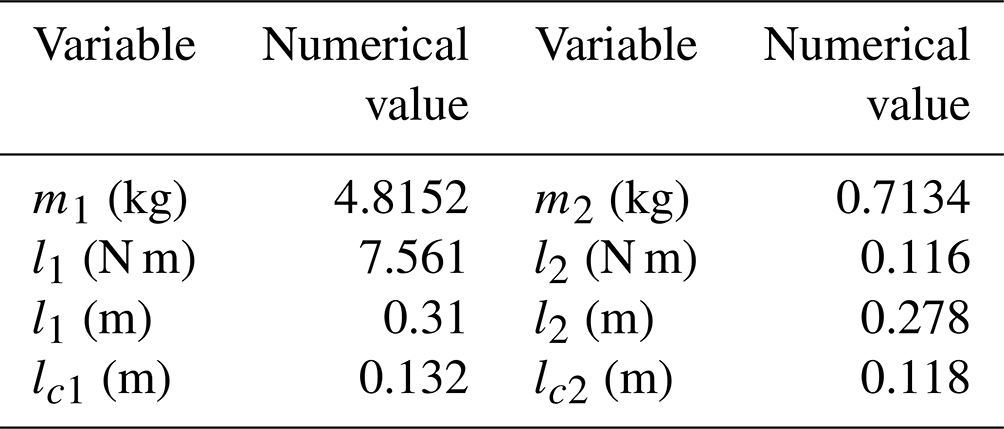
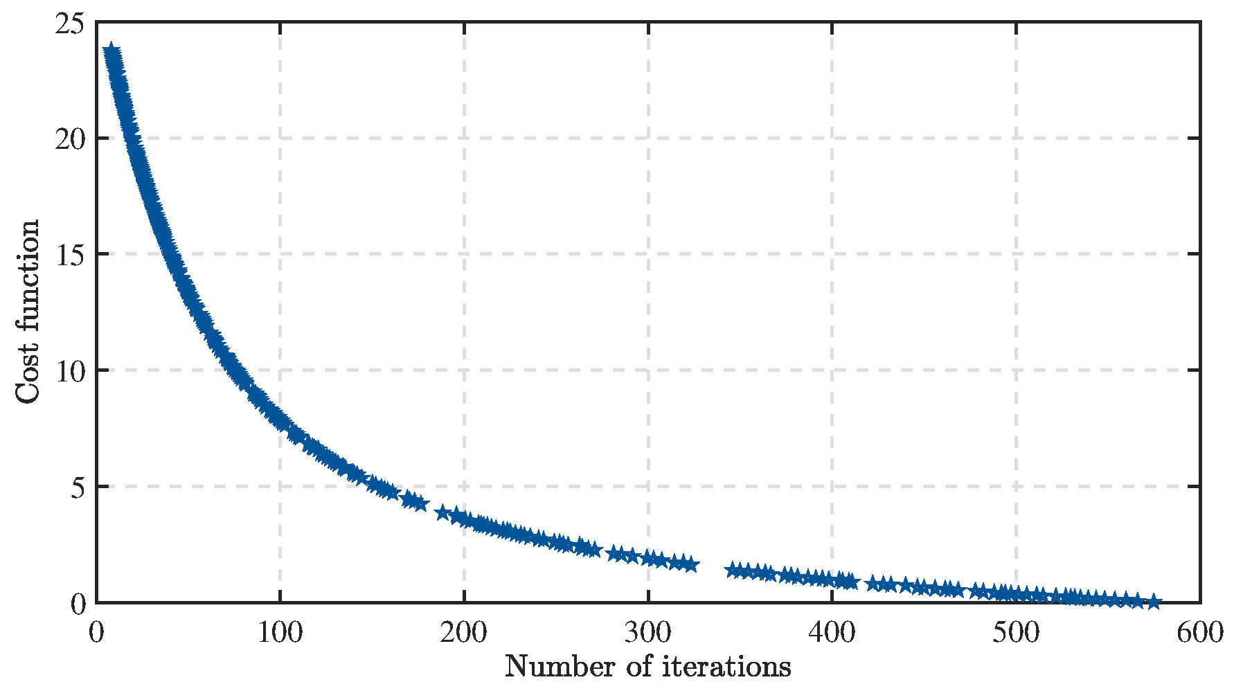
We began the process of gain learning with the nominal values of kp1nominal=10, kp2nominal=10, kd1nominal=5, and kd2nominal=5, and by adopting a constant search amplitude , , , and . As shown in Fig. 1, the learned cost function is displayed, which rapidly decreases with iteration number at the initial time and reaches a very low value after 500 iterations. At this point, the optimal control parameters for the system have also been obtained: , .
To ensure relative parity between numerical simulations and experiments, we used the identical set of system settings for both the algorithm with self-adjusting learning feedback gain (PD with robustness and feedback, PDRF) as well as the standard method and with the robust control without the feedback gain (known as PDR). This was done in order to increase the control efficacy of the system component compared to the standard PD control method.
4.1 Simulation experiment
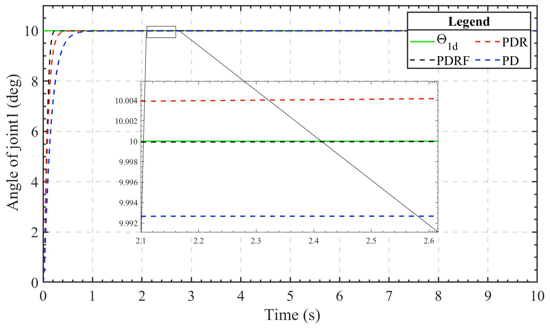
4.1.1 Step signal tracking simulation
The 2-DOF manipulator was programmed to follow the step signal with an amplitude of 10∘ in the angle variable. Figures 2 and 3 depict the displacement simulation contours of the two manipulator joints. As can be seen from the figures, under the conditions of similar dynamic performance, the transient tracking effect of the two joints under the control of PDRF is better than that under the control of PDR and PD. The advantage of PDRF is not only in tracking speed but also in tracking effectiveness. Therefore, we can see the effectiveness of the learning feedback and the robustness of the algorithm.
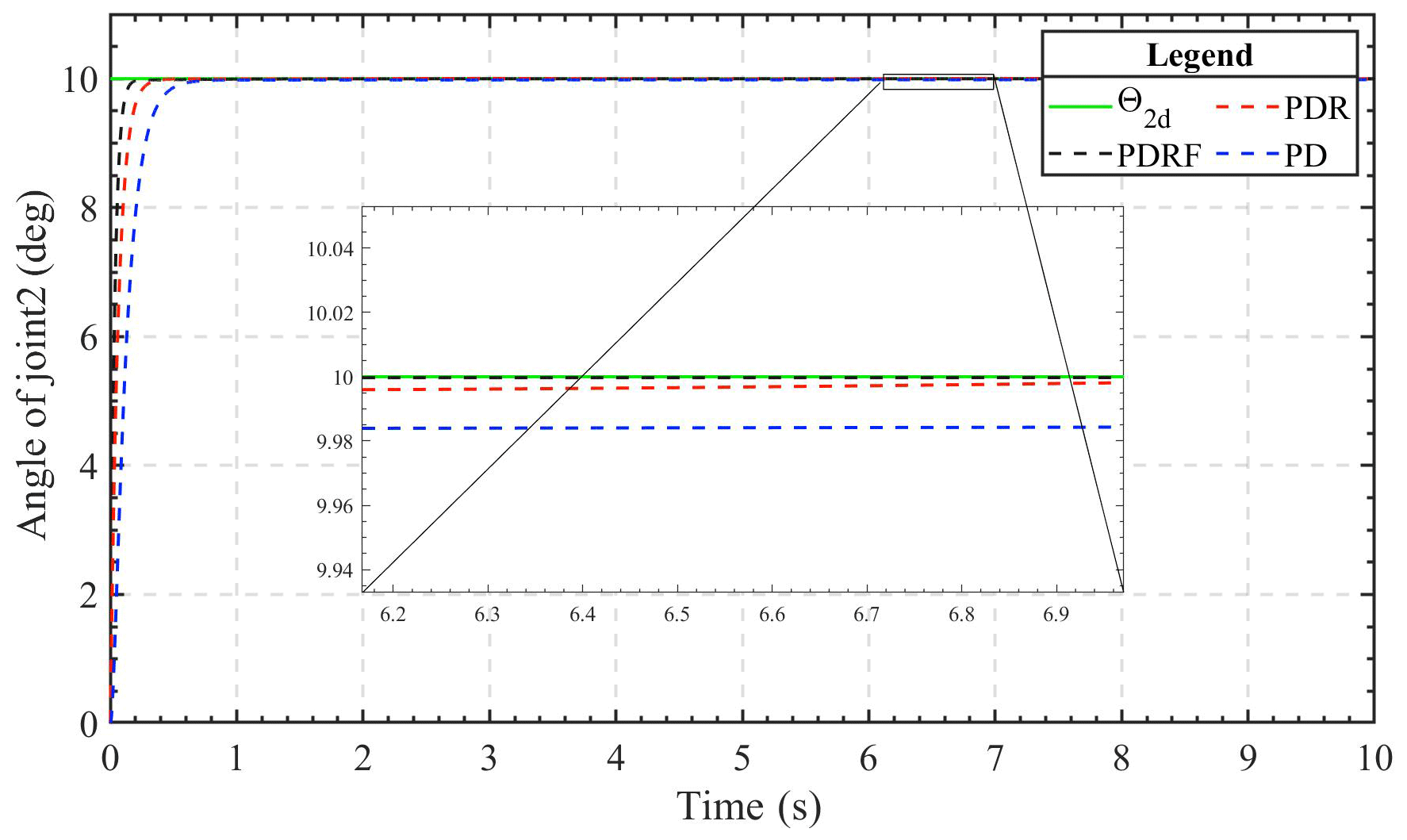
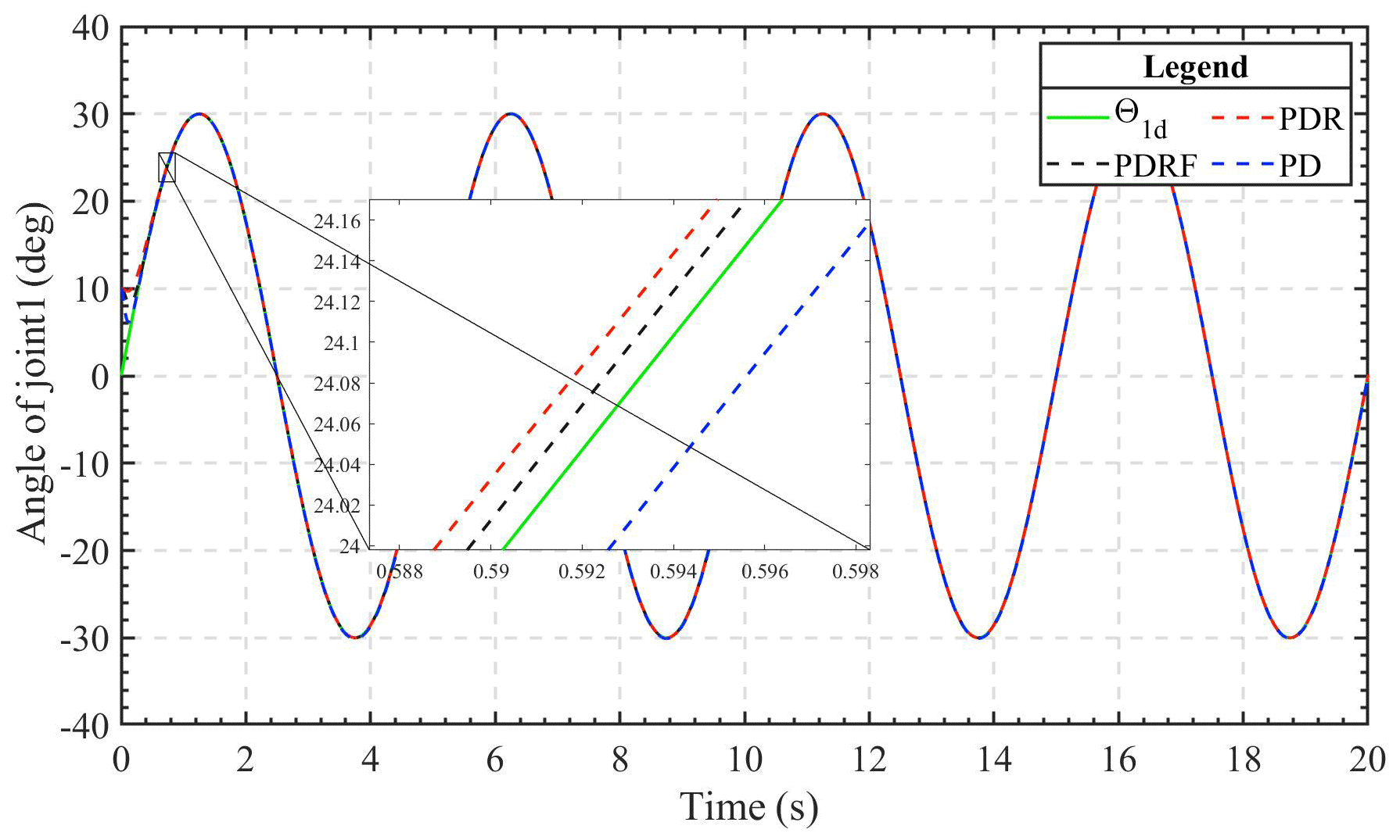
Figure 4Simulation results of joint 1 sinusoidal signal displacement tracking under different control modes.
4.1.2 Sinusoidal signal tracking simulation
The following description of the 2-DOF manipulator's predicted trajectory is offered for the purpose of conducting an investigation of the effectiveness of the control algorithm in terms of its ability to maintain a steady state while tracking a sinusoidal signal.
Figures 4 and 5 depict, respectively, the joint 1 and joint 2 trajectory tracking curves of the three different control methods. Under the same conditions and with the same controller parameters, all three of the control algorithms have the ability to track rapidly and continue to be stable fairly quickly. After the system's tracking effect stabilizes, the simulation figure's enlarged portion reveals that the PDRF controller outperforms the PD controller and PDR controller in terms of steady-state tracking, exhibiting the lowest error. This demonstrates both the effectiveness of the learned feedback gain and the robustness of the controller.
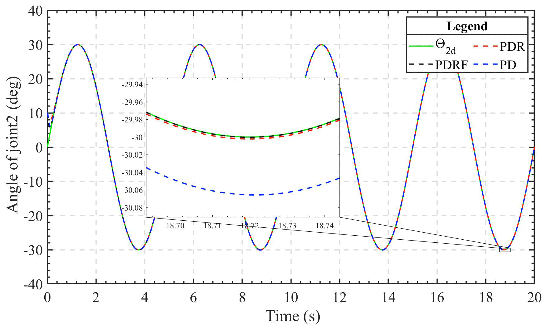
Figure 5Simulation results of joint 2 sinusoidal signal displacement tracking under different control modes.
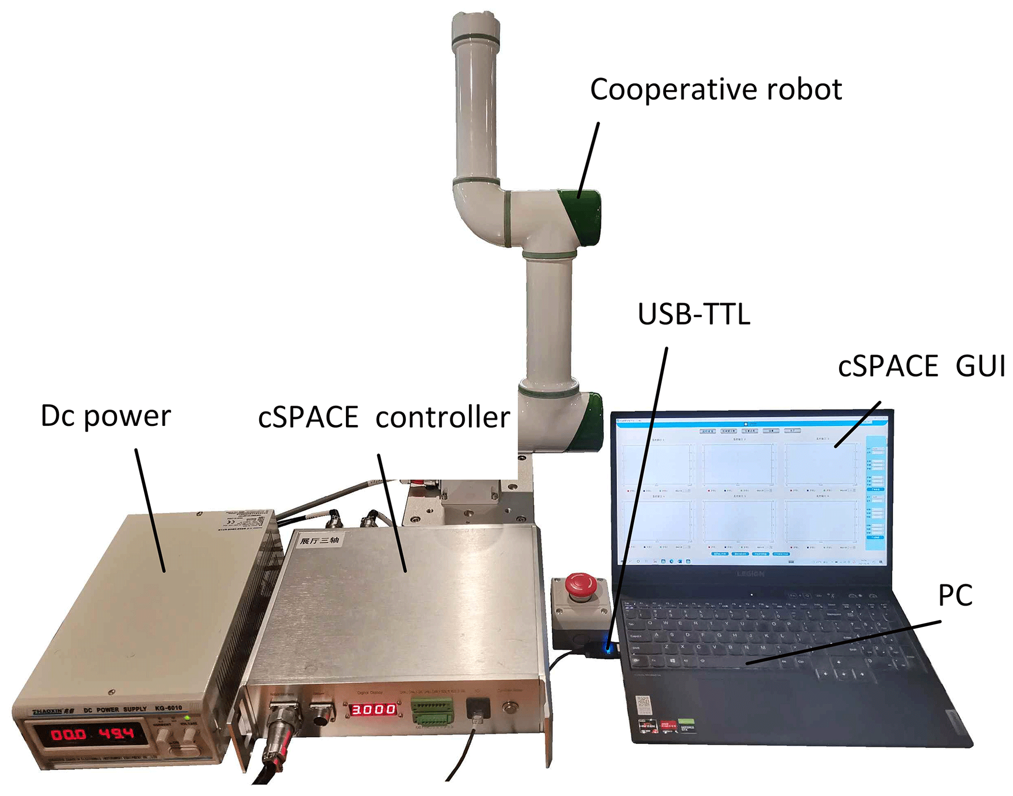
4.2 Experimental results
To verify the controller's capability of achieving high-precision trajectory tracking for the collaborative manipulator, we conducted experimental verification using a 2-DOF collaborative robot, a control system, a personal computer running MATLAB/Simulink, and a DC power supply, as shown in Fig. 6. We used the exact same experimental parameters that were used in the computational simulations so that we could be certain that the suggested approach would be effective. Experiments that included tracking step responses and tracking sinusoidal signals were carried out so that the transient tracking performance and the dynamic tracking performance of the controller could be evaluated, respectively.
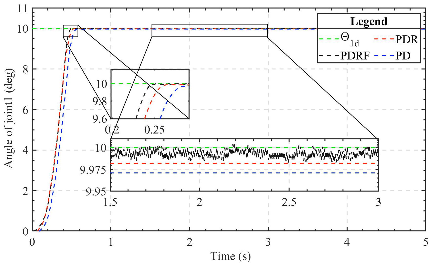
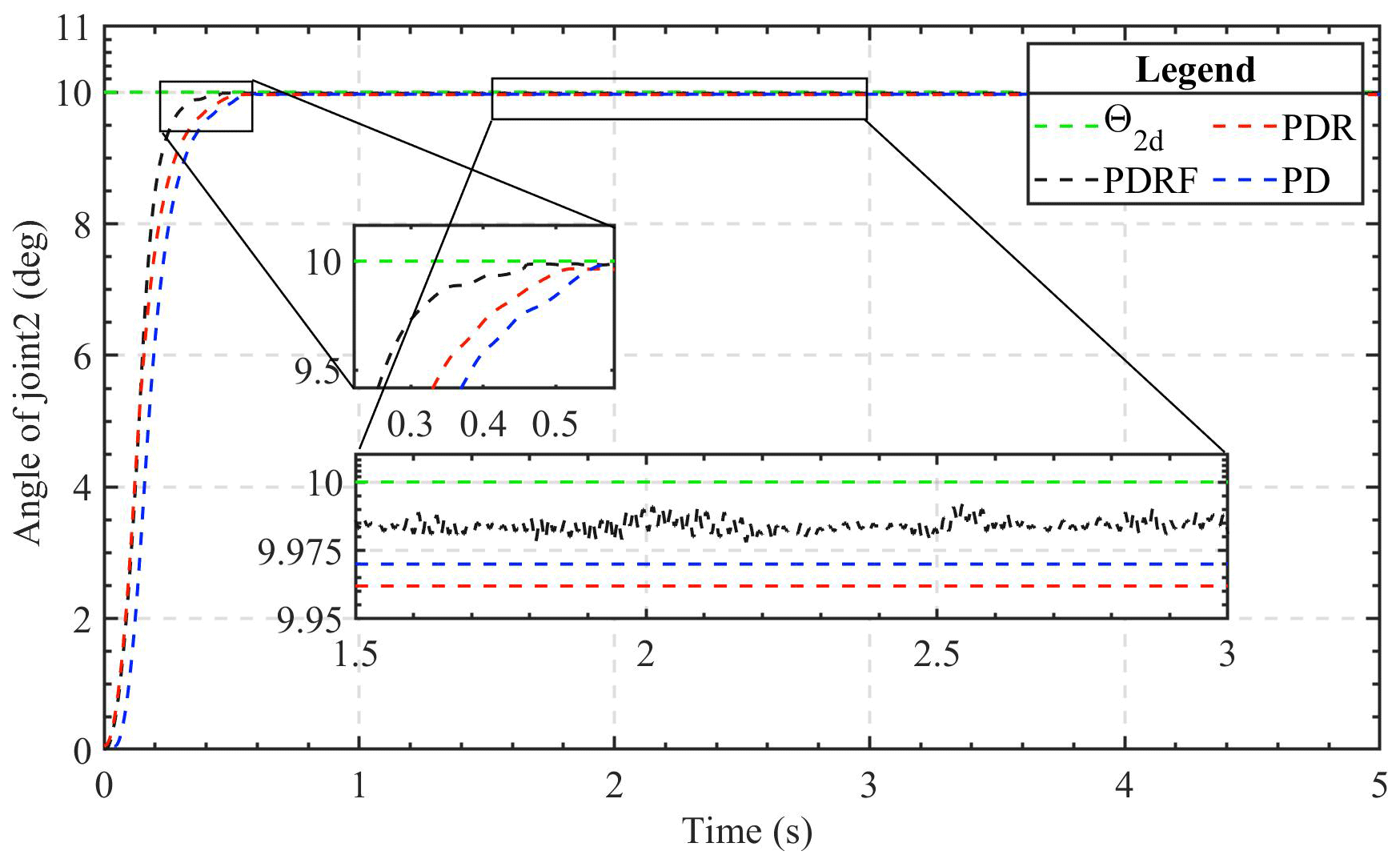
4.2.1 Step signal tracking experiment
The results of tracing the step signal are reflective of the transient performance of the controller. In light of the findings of the simulation, the 2-DOF manipulator is allowed to trace a step response signal that is 10 degrees in increments. Figures 7 and 8 depict the step response curves of the two joints under the three algorithms, respectively. When monitoring step signals, the PDRF algorithm demonstrates a faster response and a reduced steady-state error. However, there are errors during the state of dynamic change, and the learning process is a self-adjusting one. Additionally, the PDR algorithm shows a smaller steady-state error, while the traditional PD algorithm performs the worst among the three algorithms. The primary cause of the steady-state error is the system's uncertainty. Figures 7 and 8 also show that the robust feedback terms of PDR and PDRF are effective. The errors of the robust terms are all less than 0.025, while the errors of the PD algorithm are greater than 0.025. Therefore, based on comparative analysis, it is concluded that PDRF can attain a steady state faster while ensuring accuracy.
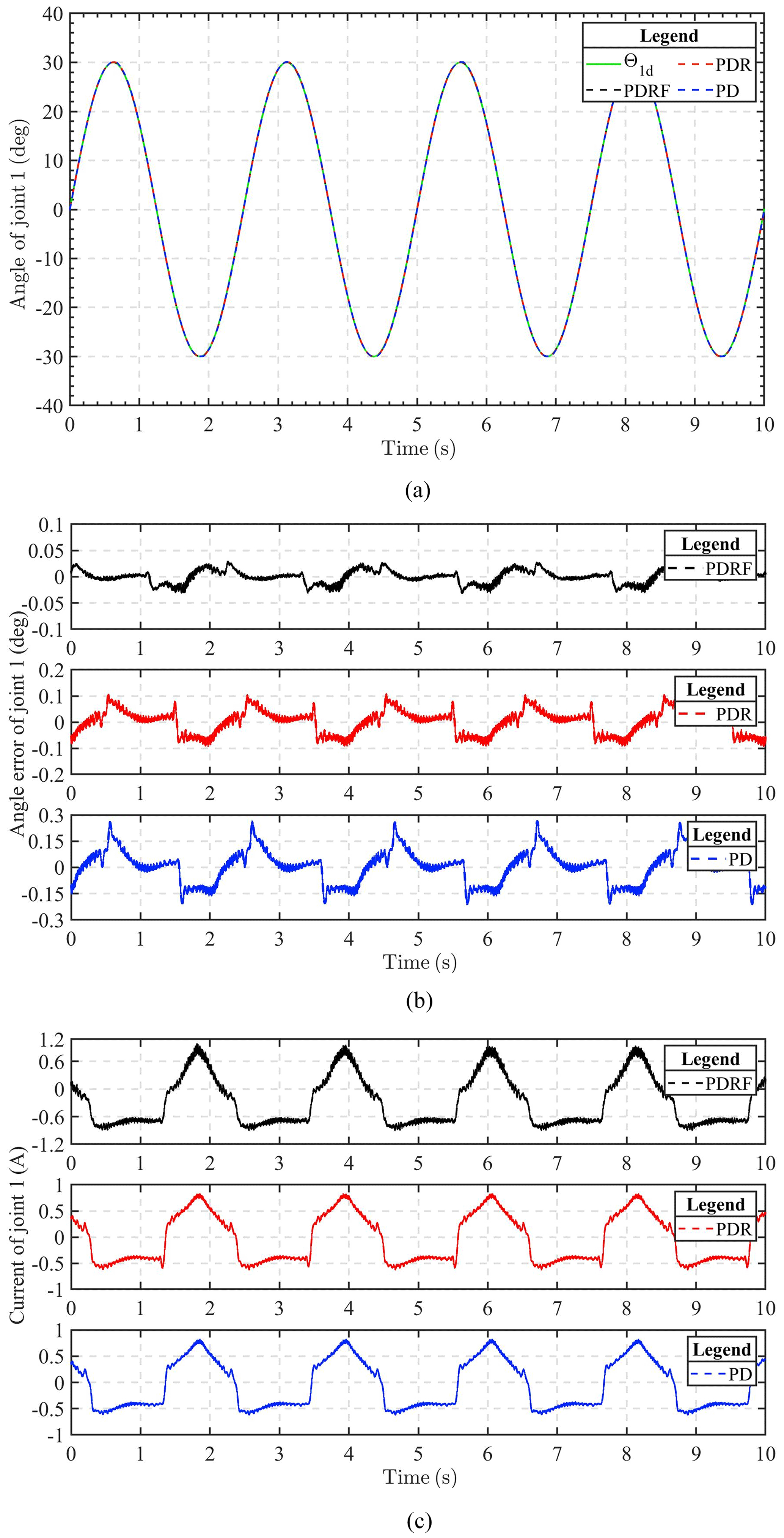
Figure 9Comparison of experimental results of sinusoidal trajectory tracking for joint 1 under different controls. (a) Experimental tracking results. (b) Tracking error. (c) Input voltage.
4.2.2 Sinusoidal tracking experiment
Figures 9 and 10 show the results of joint 1 and joint 2 under sinusoidal tracking signals, respectively, which include the tracking trajectory results, the tracking errors, and the control input of the robot system. Experiments involving the tracking of sinusoidal signals are used to validate the dynamic tracking performance of the controller.
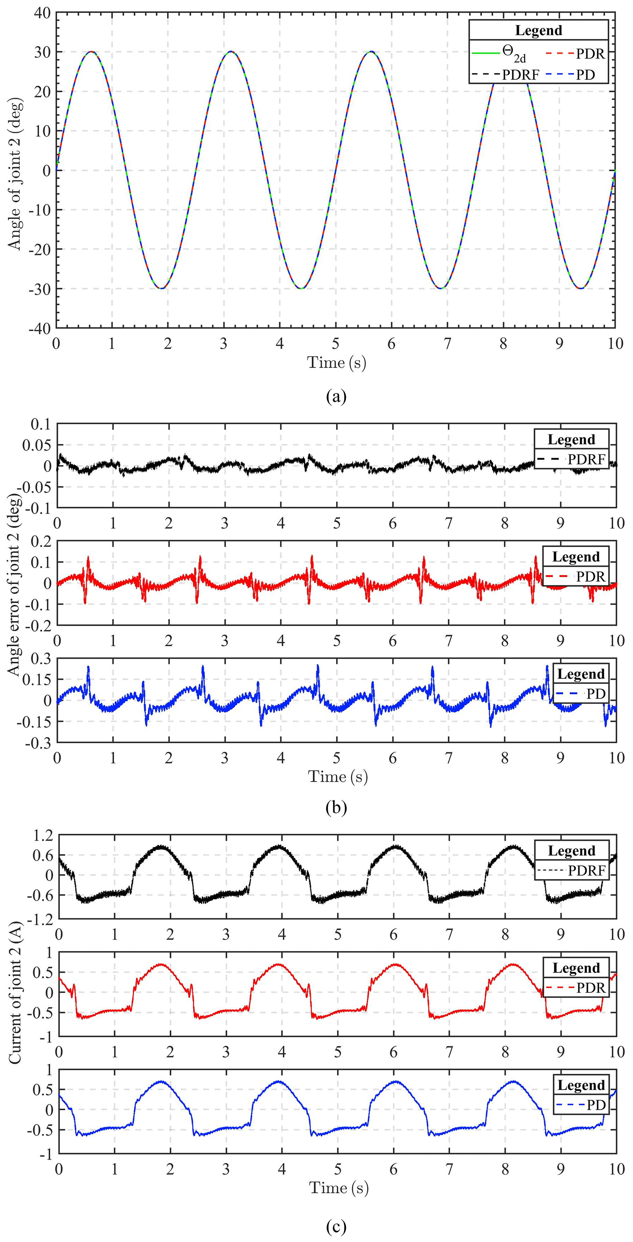
Figure 10Comparison of experimental results of sinusoidal trajectory tracking for joint 2 under different controls. (a) Experimental tracking results. (b) Tracking error. (c) Input voltage.
The experimental results show that the improved algorithm can guarantee the tracking effect. It can also be seen from these results that the steady-state error under PDRF control is less than that under PDR and PD control, within 0.05∘ in both joints, which means that PDRF control can obtain better steady-state performance. However, we can also see from Figs. 9c and 10c that a better control effect requires greater control input cost. Fortunately, the increase in cost is not particularly large and is within the acceptable range. Therefore, the control algorithm can be applied and realized in practical engineering control.
In comparison to PDR and PD controllers, our proposed algorithm (PDRF) guarantees speedier convergence and superior tracking performance, as demonstrated by the experimental results. 2-DOF experimentation verifies the robustness of 2-DOF towards uncertainty and the efficacy of autonomous adjustment of learning feedback gain.
In this paper, a robust uncertain position control algorithm for collaborative robots with automatic adjustment of the learning feedback gain is proposed to improve trajectory tracking performance. Under the PD control framework, a robust controller is designed based on the model and error, and the feedback gain is automatically adjusted by learning, so as to iteratively adjust the feedback gain and optimize the expected performance of the system. Secondly, a new robust control method with simple structure, self-adjusting parameters, and engineering practicability is proposed based on the feedback dynamic model. Theoretical analysis demonstrates that the new control method satisfies the conditions of uniform boundedness and uniform ultimate boundedness. Thirdly, simulations and experiments are conducted, and the novel control method demonstrates the desired performance, indicating that the proposed control method can considerably enhance the trajectory tracking performance of collaborative robots with uncertainties. In the next work planned, we will continue to improve and refine our method, add inequality-based error constraints, and apply and validate our proposed control algorithm on six-axis robots and other mechanical systems.
All data included in this study are available upon request by contacting the corresponding author.
MC contributed significantly to the conception and design of work, data acquisition, analysis, and interpretation. XL contributed to the acquisition of simulation experimental data and data collation.
The contact author has declared that neither of the authors has any competing interests.
Publisher’s note: Copernicus Publications remains neutral with regard to jurisdictional claims in published maps and institutional affiliations.
This research has been supported by the Innovative Research Group Project of the National Natural Science Foundation of China (grant no. 61903002), University Synergy Innovation Project of Anhui Province (grant no. GXXT-2021-050), University Outstanding Youth Research Project of Anhui Province (grant no. 2022AH020065), and Scientific Research Activities of Reserve Candidates of Academic and Technical Leaders of Anhui Province (grant no. 2022H292), as well as the Young and Middle-aged Top Talent Program of Anhui Institute of Technology and Key Research Program and Major Project of Anhui Province.
This paper was edited by Thorsten Schindler and reviewed by two anonymous referees.
Ariyur, K. B. and Krstić, M.: Slope seeking: a generalization of extremum seeking, Int. J. Adapt. Control, 18, 1–22, https://doi.org/10.1002/acs.777, 2004.
Chen, Y. H.: On the deterministic performance of uncertain dynamical systems, Int. J. Control., 43, 1557–1579, https://doi.org/10.1080/00207178608933559, 1986.
Duan, J., Shi, R., Liu, H., and Rong, H.: Design Method of Intelligent Ropeway Type Line Changing Robot Based on Lifting Force Control and Synovial Film Controller, Journal of Robotics, 2022, 3640851, https://doi.org/10.1155/2022/3640851, 2022.
Fan, Y., Zhu, Z., Li, Z., and Yang, C.: Neural Adaptive with Impedance Learning Control for Uncertain Cooperative Multiple Robot Manipulators, Eur. J. Control., 70, 100769, https://doi.org/10.1016/j.ejcon.2022.100769, 2023.
Gaidhane, P., Kumar, A., and Raj, R.: Tuning of Interval Type-2 Fuzzy Precompensated PID Controller: GWO-ABC Algorithm Based Constrained Optimization Approach, Springer Int. Pub., 75–96, https://doi.org/10.1007/978-3-031-26332-3_6, 2023.
Ghediri, A., Lamamra, K., Kaki, A. A., and Vaidyanathan, S.: Adaptive PID computed-torque control of robot manipulators based on DDPG reinforcement learning, International Journal of Modelling, Identification and Control (IJMIC), 41, 173–182, https://doi.org/10.1504/ijmic.2022.10052625, 2022.
Guo, Q., Zhang, Y., Celler, B. G., and Su, S. W.: Backstepping control of electro-hydraulic system based on extended-state-observer with plant dynamics largely unknown, IEEE T. Ind. Electron., 63, 6909–6920, https://doi.org/10.1109/TIE.2016.2585080, 2016.
Guo, Q., Yin, J., Yu, T., and Jiang, D.: Saturated adaptive control of an electrohydraulic actuator with parametric uncertainty and load disturbance, IEEE T. Ind. Electron., 64, 7930–7941, https://doi.org/10.1109/TIE.2017.2694352, 2017.
Jiang, B., Karimi, H. R., Yang, S., Gao, C., and Kao, Y.: Observer-based adaptive sliding mode control for nonlinear stochastic Markov jump systems via T–S fuzzy modeling: Applications to robot arm model, IEEE T. Ind. Electron., 68, 466–477, https://doi.org/10.1109/tie.2020.2965501, 2020.
Jie, W., Yu, D. Z., Yu, L. B., Kim, H. H., and Lee, M. C.: Trajectory tracking control using fractional-order terminal sliding mode control with sliding perturbation observer for a 7-DOF robot manipulator, IEEE-ASME T. Mech., 25, 1886–1893, https://doi.org/10.1109/tmech.2020.2992676, 2020.
Khaled, T. A., Akhrif, O., and Bonev, I. A.: Dynamic path correction of an industrial robot using a distance sensor and an ADRC controller, IEEE-ASME T. Mech., 26, 1646–1656, https://doi.org/10.1109/tmech.2020.3026994, 2020.
Kong, L., He, W., Yang, C., and Sun, C.: Robust neurooptimal control for a robot via adaptive dynamic programming, IEEE T. Neur. Net. Lear., 32, 2584–2594, https://doi.org/10.1109/tnnls.2020.3006850, 2020.
Krstić, M. and Wang, H. H.: Stability of extremum seeking feedback for general nonlinear dynamic systems, Automatica, 36, 595–601, https://doi.org/10.1016/s0005-1098(99)00183-1, 2000.
Li, F., Zhang, Z., Wu, Y., Chen, Y., Liu, K., and Yao, J.: Improved fuzzy sliding mode control in flexible manipulator actuated by PMAs, Robotica, 40, 2683–2696, https://doi.org/10.1017/s0263574721001909, 2022.
Lv, Z.: Simulation of grasping attitude control of robotic arm based on synovial error feedback, Int. J. Ind. System., 36, 110–124, https://doi.org/10.1504/ijise.2020.10024654, 2020.
Lytridis, C., Kaburlasos, V. G., and Pachidis, T.: An overview of cooperative robotics in agriculture, Agronomy, 11, 1818, https://doi.org/10.3390/agronomy11091818, 2021.
Ma, L., Yan, Y., and Li, Z.: A novel aerial manipulator system compensation control based on ADRC and backstepping, Sci. Rep.-UK., 11, 22324, https://doi.org/10.1038/s41598-021-01628-1, 2021.
Muñoz-Vázquez, A. J., Gaxiola, F., and Martínez-Reyes, F.: A fuzzy fractional-order control of robotic manipulators with PID error manifolds, App. Soft. Comput., 83, 105646, https://doi.org/10.1016/j.asoc.2019.105646, 2019.
Niu, X., Yang, C., Tian, B., Li, X., and Han, J.: Modal decoupled dynamics feed-forward active force control of spatial multi-dof parallel robotic manipulator, Math. Probl. Eng., 2019, 1835308, https://doi.org/10.1155/2019/1835308, 2019.
Ramuzat, N., Boria, S., and Stasse, O.: Passive inverse dynamics control using a global energy tank for torque-controlled humanoid robots in multi-contact, IEEE Robot. Autom. Let., 7, 2787–2794, https://doi.org/10.1109/lra.2022.3144767, 2022.
Regmi, S., Burns, D., and Song, Y. S.: Humans modulate arm stiffness to facilitate motor communication during overground physical human-robot interaction, Sci. Rep.-UK., 12, 18767, https://doi.org/10.1038/s41598-022-23496-z, 2022.
Ryu, J. H., Kwon, D. S., and Park, Y.: A robust controller design method for a flexible manipulator with a large time varying payload and parameter uncertainties, J. Intell. Robot. Syst., 27, 345–361, https://doi.org/10.1109/robot.1999.770013, 2000.
Salman, M., Khan, H., and Lee, M. C.: Perturbation Observer-Based Obstacle Detection and Its Avoidance Using Artificial Potential Field in the Unstructured Environment, Appl. Sci., 13, 943, https://doi.org/10.3390/app13020943, 2023.
Xian, Y., Huang, K., Zhen, S., Wang, M., and Xiong, Y.: Task-Driven-Based Robust Control Design and Fuzzy Optimization for Coordinated Robotic Arm Systems, Int. J. Fuzzy Syst., 25, 1579–1596, https://doi.org/10.1007/s40815-023-01460-x, 2023.
Xiao, W., Chen, K., Fan, J., Hou, Y., Kong, W., and Dan, G.: AI-driven rehabilitation and assistive robotic system with intelligent PID controller based on RBF neural networks, Neural Comput. Appl., 1–15, https://doi.org/10.1007/s00521-021-06785-y, 2022.
Xu, K. and Wang, Z.: The design of a neural network-based adaptive control method for robotic arm trajectory tracking, Neural Comput. Appl., 35, 8785–8795, https://doi.org/10.1007/s00521-022-07646-y, 2023.
Yin, X. and Pan, L.: Enhancing trajectory tracking accuracy for industrial robot with robust adaptive control, Robot. CIM-Int. Manuf., 51, 97–102, https://doi.org/10.1016/j.rcim.2017.11.007, 2018.
Zaiwu, M., Li, P. C., and Jian, W. D.: Feed-forward control of elastic-joint industrial robot based on hybrid inverse dynamic model, Adv. Mech. Eng., 13, 9, https://doi.org/10.1177/16878140211038102, 2021.
Zhai, A., Wang, J., Zhang, H., Lu, G., and Li, H.: Adaptive robust synchronized control for cooperative robotic manipulators with uncertain base coordinate system, ISA T., 126, 134–143, https://doi.org/10.1016/j.isatra.2021.07.036, 2022.
Zhang, F.: High-speed nonsingular terminal switched sliding mode control of robot manipulators, IEEE/CAA Journal of Automatica Sinica, 4, 775–781, https://doi.org/10.1109/jas.2016.7510157, 2016.
Zhang, R., Wang, Z., Bailey, N., and Keogh, P.: Experimental assessment and feedforward control of backlash and stiction in industrial serial robots for low-speed operations, Int. J. Comput. Integ. M., 36, 393–410, https://doi.org/10.1080/0951192x.2022.2090609, 2022.
Zhao, H., Tao, B., Ma, R., and Chen, B.: Manipulator trajectory tracking based on adaptive sliding mode control, Concurr. Comp.-Pract. E., 34, e7051, https://doi.org/10.1002/cpe.7051, 2022.
Zhen, S., Zhao, Z., Liu, X., Chen, F., Zhao, H., and Chen, Y. H.: A novel practical robust control inheriting PID for SCARA robot, IEEE Access, 8, 227409–227419, https://doi.org/10.1109/access.2020.3045789, 2020.
Zhong, G., Wang, C., and Dou, W.: Fuzzy adaptive PID fast terminal sliding mode controller for a redundant manipulator, Mech. Syst. Signal. Pr., 159, 107577, https://doi.org/10.1016/j.ymssp.2020.107577, 2021.