Intelligent vehicle obstacle avoidance path-tracking control based on adaptive model predictive control

In order to solve the problems of low path-tracking accuracy, poor safety, and stability of intelligent vehicles with variable speeds and obstacles on the road, a double-layer adaptive model predictive controller (MPC) is designed. A vehicle point mass model is used in an obstacle avoidance planning controller, and the safety collision distance model is established according to the distance relationship between the vehicle and the obstacle to improve the driving safety of the vehicle. The design of the path-tracking controller is based on the three-degrees-of-freedom dynamics model. According to the relationship between the predictive horizon and vehicle speed in the MPC algorithm, an adaptive path-tracking control strategy which can update the prediction horizon in real time is proposed to improve the accuracy of vehicle path tracking. To increase the vehicle stability, a sideslip angle and an acceleration control variable are added to the vehicle dynamics model as soft constraint conditions. The proposed method is simulated based on a CarSim and MATLAB/Simulink co-simulation platform. The simulation results show that the maximum lateral path deviation and the maximum centroid sideslip angle of the designed controller are 0.13 m and 0.4^∘, respectively. Compared with the traditional MPC, the adaptive MPC maximum lateral path deviation and the maximum centroid sideslip angle are reduced by 0.51 m and 1.57^∘, respectively, which proves the effectiveness of the proposed method.

1 Introduction

With the rapid development of artificial intelligence and sensor technology, intelligent vehicle technology has made great progress. Obstacle avoidance planning and path-tracking control are the key technologies of intelligent vehicle automatic driving. Obstacle avoidance planning calculates a safe and stable driving path based on the information about obstacles. Path-tracking control ensures that the vehicle can accurately track the reference path. Therefore, the intelligent vehicle obstacle avoidance path-tracking control has become a research hotspot in recent years.

On the path-tracking control problem, Gutjahr et al. (2016) proposed a linear time-varying MPC control method, but the method is based on the kinematic model without considering the vehicle dynamics constraints. Mata et al. (2018) presented a trajectory-tracking control method based on multiple constraints, and the continuous linearization error model and quadratic programming were used to obtain a good trajectory-tracking effect. Liu et al. (2018) proposed a hierarchical vision-based lateral-control scheme, and the controller is designed by a robust H∞-based linear quadratic regulator (LQR) algorithm to compensate for sensor-induced delays. Mata et al. (2018) and Liu et al. (2018) did not take into account the view of obstacles in the actual driving process of the vehicle. On the obstacle avoidance planning problem, Karaman et al. (2011) proposed an anytime algorithm based on RRT^* to generate the planned path, but the stability of the algorithm was not considered. The stability of the algorithm will affect the convergence time and whether the generated path can converge to the global optimal path. Tomas-Gabarron et al. (2013) converted the obstacle avoidance route of intelligent vehicles into a multitasking objective problem and computed the safe obstacle avoidance path. Chen et al. (2019) switched the path-planning problem of intelligent vehicles to the problem solved by the Bezier curve and the feasible planning path obtained by a genetic algorithm. The obstacle avoidance planning algorithm proposed by Tomas-Gabarron et al. (2013) and Chen et al. (2019) has a lot of computation, and the model is complex. Considering the real road conditions in the process of intelligent vehicle driving and the large amount of calculation in obstacle avoidance planning and path-tracking control, a simplified vehicle model should be adopted in this paper.

On the joint problem of obstacle avoidance planning and path-tracking control, the sensing module, including vehicle sensors, cameras, and radar modules, detects the position coordinates of obstacles on the road in real time and sends the coordinate information to the obstacle avoidance planning layer. The obstacle avoidance planning layer uses the coordinate information to calculate and give the optimal path, and then the path-tracking control layer controls the vehicle to drive along the path. Li et al. (2018) presented an integrated method of trajectory planning and control based on a nonlinear vehicle model predictive control algorithm and improved the four-wheel dynamics model and nonlinear tire model. Xu et al. (2020) proposed a powerful hierarchical path-planning and trajectory-tracking framework. For path planning, considering vehicle kinematics, a feasible and collision-free trajectory is generated. For path tracking, the front-wheel steering angle is obtained by solving the constraint model predictive control problem. Zuo et al. (2021) proposed a progressive model predictive control scheme in which the cooperative control of local planning and path tracking of intelligent vehicles is considered. The model predictive control is combined with the artificial potential field method. The above two methods have had a lot of research on the obstacle avoidance path-tracking control of intelligent vehicles. However, in actual driving, the vehicle is often in a variable speed state, and there are obstacles in the road. Thus, driving safety and stability are being challenged. We propose an adaptive double-layer model predictive control strategy for intelligent vehicle obstacle avoidance planning and path-tracking control in this paper, and the feasibility of the proposed control strategy is verified by simulation. The innovation and contribution of this paper are as follows.

• I.

  To ensure the security of the intelligent vehicle obstacle avoidance trajectory-tracking control, an obstacle avoidance function is designed in the controller based on the relationship between obstruction and vehicle location, and a safe collision distance model is built.

• II.

  A double-layer adaptive variable prediction horizon obstacle avoidance route-tracking controller is created, and an adaptive variable prediction horizon control approach is suggested. The controller can increase the accuracy of intelligent vehicle path tracking by calculating the best prediction horizon in real time in response to changes in vehicle speed.

• III.

  Sideslip angle and acceleration control variables are introduced into the vehicle dynamics model as soft constraints to improve vehicle stability for intelligent vehicle driving.

2 Vehicle model

2.1 Point mass model

In order to avoid obstacles on the road, the intelligent vehicle obstacle avoidance planning controller needs to plan a feasible target path based on the position information between the vehicle and the obstacle. In the process of obstacle avoidance planning and path-tracking control of intelligent vehicles, the calculation amount of the algorithm in the obstacle avoidance planning controller is large. In the obstacle avoidance planning controller, the vehicle running on the planning reference path can be regarded as a mass point, so the vehicle point mass model is adopted, which not only simplifies the model, but also reduces the amount of calculation (Li et al., 2020). The vehicle point mass model diagram is shown in Fig. 1.

Figure 1 Vehicle point mass model.

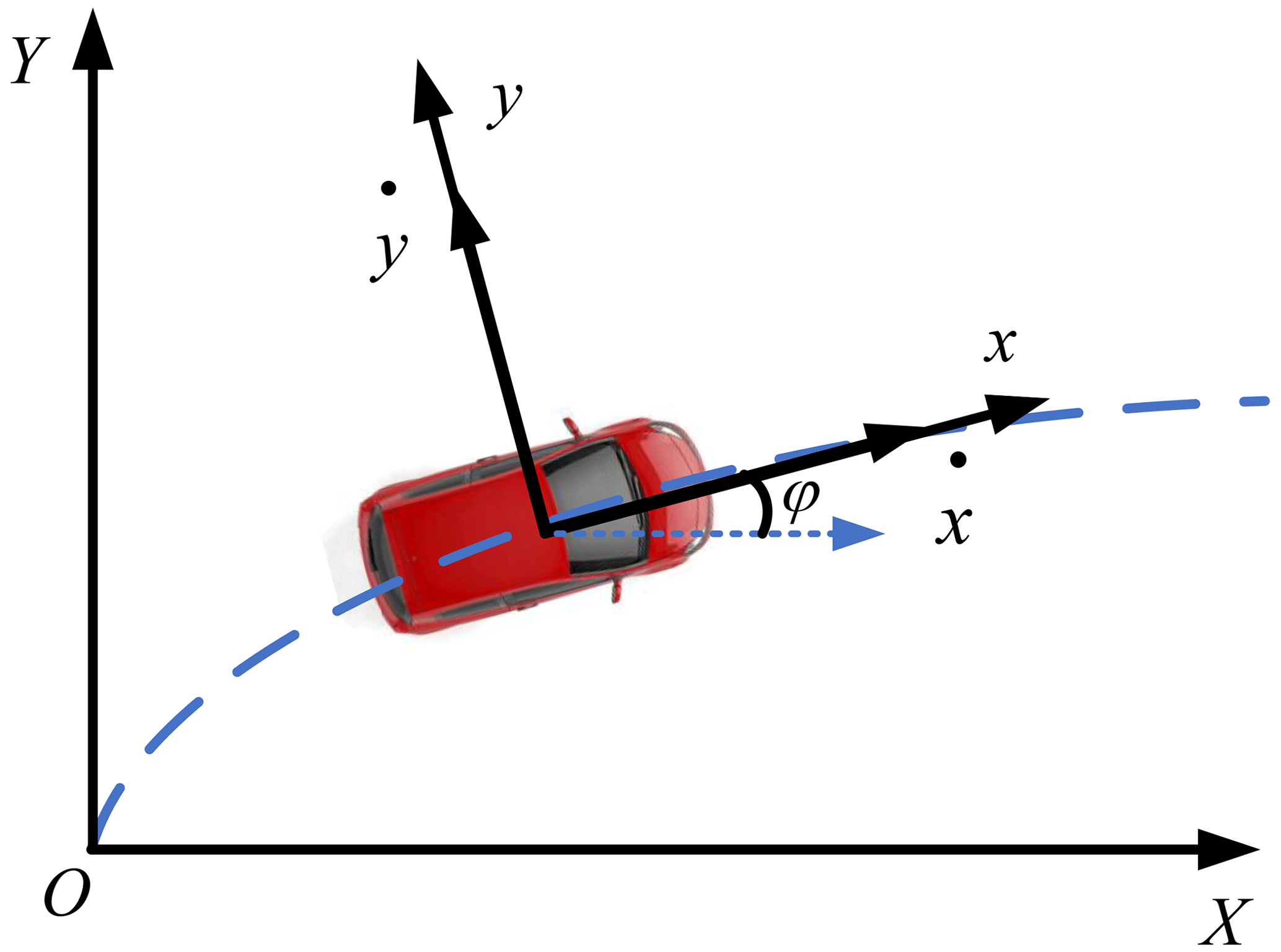
In the established reference coordinate system, the vehicle point mass model can be expressed as

$$\begin{array}{}\text{(1)}& {\displaystyle }\dot{X}=\dot{x}\cos \mathit{\psi }-\dot{y}\sin \mathit{\psi },\text{(2)}& {\displaystyle }\dot{Y}=\dot{x}\sin \mathit{\psi }+\dot{y}\cos \mathit{\psi },\end{array}$$

where $\dot{X}$ and $\dot{Y}$ are the longitudinal and transverse velocities in the inertial coordinate system, respectively. $\dot{x}$ and $\dot{y}$ are the longitudinal and transverse velocities in the vehicle coordinate system, respectively. ψ is the vehicle's course angle.

2.2 Three-degrees-of-freedom dynamics model

Considering the longitudinal, lateral, and yaw motions of the vehicle, the point mass model is no longer suitable for vehicle path-tracking control (Bobier-Tiu et al., 2019; Kucuk, 2017). In order to make the vehicle track the planned path quickly and accurately under high-speed driving conditions, it is necessary to establish a vehicle dynamics model that can accurately describe the vehicle's motion state in the path-tracking controller. Figure 2 shows a three-degrees-of-freedom dynamics model of a vehicle.

Figure 2 Three-degrees-of-freedom dynamics model.

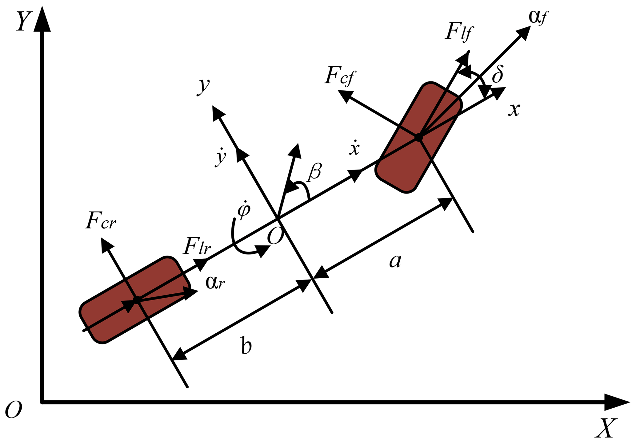
Assuming that the vehicle travels on a horizontal road and ignores the effect of air resistance, the vehicle dynamics equation based on Newton's second law is as follows (Nan et al., 2021; Woo et al., 2021).

$$\begin{array}{}\text{(3)}& {\displaystyle }m\ddot{x}=m\dot{y}\dot{\mathit{\phi }}+\mathrm{2}\left(F_{\mathrm{lf}}+F_{\mathrm{cf}}\mathit{\delta }+F_{\mathrm{lr}}\right),\text{(4)}& {\displaystyle }m\ddot{y}=\mathrm{2}\left(F_{\mathrm{cf}}+F_{\mathrm{cr}}\right)-m\dot{x}\dot{\mathit{\phi }},\text{(5)}& {\displaystyle }{I}_z\ddot{\mathit{\phi }}=\mathrm{2}\left(a{F}_{\mathrm{cf}}-b{F}_{\mathrm{cr}}\right),\end{array}$$

where m is the vehicle body mass, I_z is the vehicle yaw moment of inertia, $\ddot{\mathit{\phi }}$ is the yaw angle acceleration, δ is the front wheel angle, $\dot{\mathit{\phi }}$ is the heading angle acceleration, and a and b are the distances between the vehicle centroid and the front and rear axles, respectively. F_lf and F_lr are the longitudinal forces of the front and rear tires, respectively. F_cf and F_cr are the lateral forces of the front and rear tires, respectively. $\ddot{x}$ and $\ddot{y}$ are the longitudinal and transverse accelerations in the vehicle coordinate system, respectively.

3 Design of the obstacle avoidance planning controller

In order to make the vehicle meet the requirements of obstacle avoidance in path tracking (Cheng et al., 2020), as shown in Fig. 3, a double-layer adaptive MPC obstacle avoidance planning and path-tracking control strategy is designed. The upper controller is based on the vehicle point mass model. The controller avoids obstacles according to the position information of vehicles and obstacles. The under-layer controller is based on the vehicle dynamics model, and the target path is tracked by controlling the front wheel angle and the speed change.

Figure 3 Double-layer adaptive MPC structure.

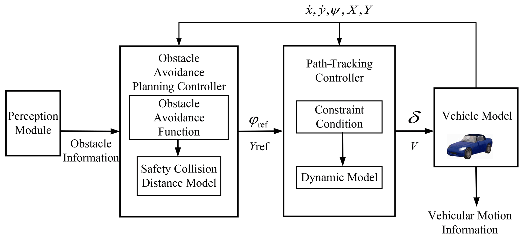
Firstly, after the obstacle avoidance planning layer receives the obstacle information from the sensor module, the obstacle information in the form of discrete points is calculated into a curve by the five-times fitting polynomial method (Li et al., 2019). Secondly, the obstacle avoidance planning layer outputs the curve information to the path-tracking control layer. Also, the path-tracking control layer receives the curve information and constructs a traceable path. Finally, the front wheel angle is used as the control output to control the vehicle to track this executable path in the path-tracking control layer.

3.1 Establishment of the safety collision distance model

The intelligent vehicle environment perception module detects obstacles on the road in real time (these obstacles may suddenly appear), and the perception module sends obstacle information to the obstacle avoidance planning controller. The obstacle avoidance planning controller uses the safe obstacle avoidance model designed in this paper to re-plan a safe driving path to ensure vehicle driving safety. The obstacle is treated with expansion with the aim of preventing vehicles from crossing it. The extension method measures the radius of the outer circle of the obstacle and the vehicle motion center as the extension size and the safe distance, respectively. When the vehicle runs at a constant speed, the distance between the vehicle and the obstacle can be expressed as L=vt. If the vehicle speed is too fast or the distance between the vehicle and the obstacle is too close, the safety of the vehicle will be greatly reduced. The safety distance of the vehicle running at a constant speed is designed as

$$\begin{array}{}\text{(6)}& L=kvt+l_{\mathrm{0}},\end{array}$$

where k is the safety factor, l₀ is the minimum distance between the vehicle and the obstacle, v is the vehicle speed, and t is the vehicle driving time.

In general, the speed of the vehicle changes during driving. In order to improve the vehicle safety, an anti-collision constraint condition needs to be added on the basis of obstacle expansion. The anti-collision constraint is established as follows.

$$\begin{array}{}\text{(7)}& (R+r{)}^{\mathrm{2}}<{\left[X\left(t\right)-x_i\right]}^{\mathrm{2}}+{\left[Y\left(t\right)-y_i\right]}^{\mathrm{2}},\end{array}$$

where X(t) and Y(t) are, respectively, the lateral and longitudinal coordinates of the vehicle at time t. The center circumcircle radii of the vehicle and the obstacle are R and r, respectively. (x_i,y_i) is the center coordinate of the obstacle. Figure 4 is a safe collision distance model, which takes into account both uniform and variable speeds. When the vehicle runs at a constant speed, the controller adopts a safety distance model (Jeong, 2021). When the vehicle speed changes, the controller applies the anti-collision constraint conditions to the vehicle.

Figure 4 Vehicle safety collision distance model.

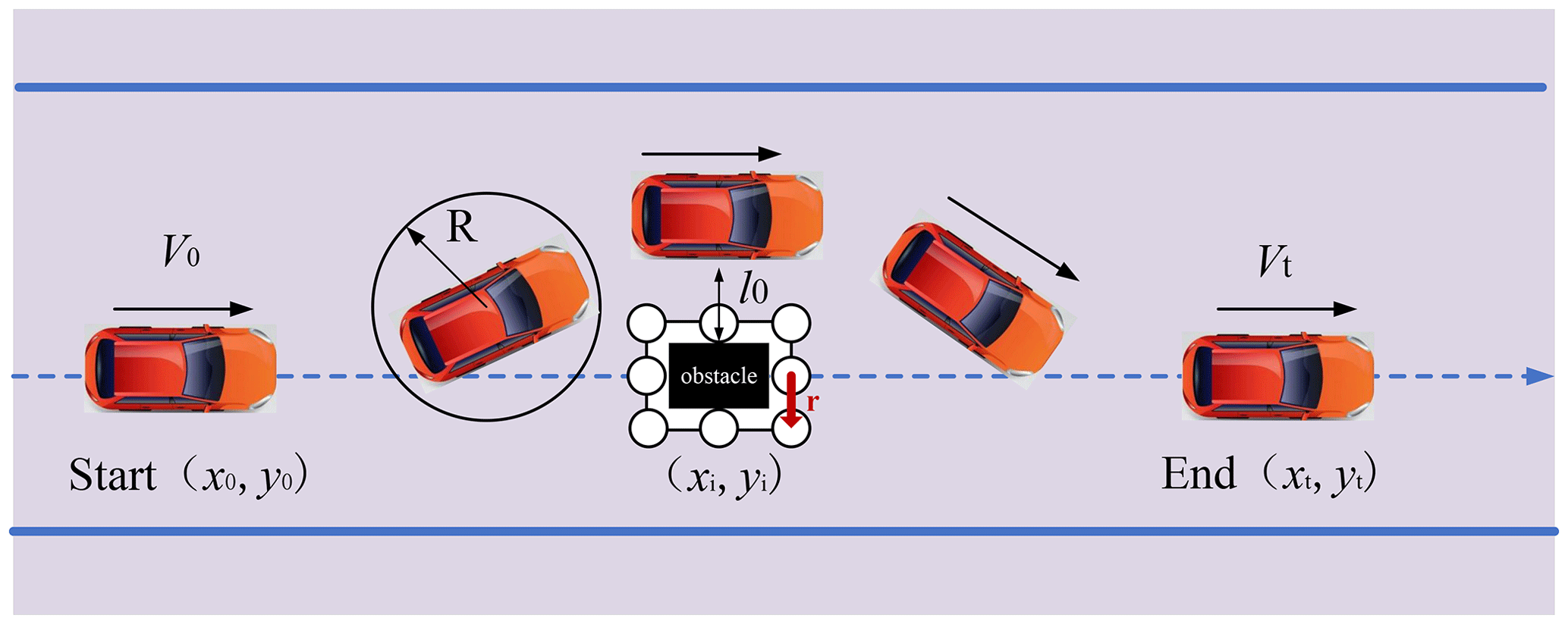
(x₀,y₀) is the vehicle starting center point coordinate, (x_t,y_t) is the vehicle ending center point coordinate, and (x_i,y_i) is the center point coordinate of the obstacle.

3.2 Obstacle avoidance function

When there are obstacles in the reference path, the obstacle avoidance function is designed to describe the distance relationship between the vehicle and the obstacle; combined with the influence of vehicle speed, the expression of the obstacle avoidance function is given:

$$\begin{array}{}\text{(8)}& J_{\mathrm{obs},i}={\displaystyle \frac{S_{\mathrm{obs}}\left(v_x^{\mathrm{2}}+v_y^{\mathrm{2}}\right)}{{\left(x_i-x_{\mathrm{0}}\right)}^{\mathrm{2}}+{\left(y_i-y_{\mathrm{0}}\right)}^{\mathrm{2}}+\mathit{\epsilon }}},\end{array}$$

where S_obs is the weight coefficient, and ε is a constant (in order to prevent the denominator from being zero). It can be seen from Eq. (8) that the vehicle is closer to the obstacle, and the function value is larger. When the vehicle is farther away from the obstacle, the function value is smaller, which means that the vehicle is in a safe position.

3.3 Establishing the target function

According to the requirements of the path-tracking control, the distance between the actual driving path and the reference path of the vehicle should be reduced as much as possible. The re-planning path can be expressed by the following target function:

$$\begin{array}{}\text{(9)}& \begin{array}{rl}J\left(t\right)& =\underset{U_t}{min}\sum _{i=\mathrm{1}}^{H_{\mathrm{p}}}\left|\right|\mathit{\eta }(t+\mathrm{1}|t)-{\mathit{\eta }}_{\mathrm{ref}}(t+\mathrm{1}\left|t\right)|{|}_Q^{\mathrm{2}}+|\left|U_i\right|{|}_R^{\mathrm{2}}\\ & +S{j}_{\mathrm{obs},i},\end{array}\end{array}$$

where H_p is the predictive horizon, U_i is the control variable in the prediction horizon, Q is the output weight, R is the input weight, and η_ref is the reference path point.

3.4 Five-times polynomial fitting

According to the target function of the obstacle avoidance planning controller, the re-planning path is composed of discrete points. When these points are transmitted to the path-tracking controller, it is necessary to fit these discrete points with a five-times polynomial.

$$\begin{array}{}\text{(10)}& \begin{array}{rl}{y}_{\mathrm{ref}}& =\sum _{i=\mathrm{0}}^{\mathrm{5}}{p}_i{x}^i\\ & =p_{\mathrm{0}}+p_{\mathrm{1}}{x}^{\mathrm{1}}+p_{\mathrm{2}}{x}^{\mathrm{2}}+p_{\mathrm{3}}{x}^{\mathrm{3}}+p_{\mathrm{4}}{x}^{\mathrm{4}}+p_{\mathrm{5}}{x}^{\mathrm{5}},\end{array}\end{array}$$

where y_ref and x are the lateral and longitudinal positions of the vehicle under the reference path, respectively. p is the polynomial coefficient.

4 Design of the path-tracking controller

The path-tracking control problem is essentially a vehicle steering-wheel angle control problem, also known as the vehicle lateral-control problem. Based on the reference path information input by the path-planning layer, according to the current state of the vehicle, the optimal control quantity is calculated and output to the execution layer. Finally, through the accurate execution of the actuator, the vehicle path-tracking control is completed.

4.1 Linearized system

Combined with the vehicle dynamics model in Eqs. (3)–(5), the design of the path-tracking controller can be expressed as the following state space expressions.

$$\begin{array}{}\text{(11)}& \stackrel{\mathrm{̃}}{x}=f(x,u),y=\mathbf{C}x,\end{array}$$

where x represents the state value, $x=\left[\dot{y}\dot{x}\mathit{\phi }\dot{\mathit{\phi }}YX\right]$, u represents the front-wheel angle control value, y represents the output value, and C is the output matrix.

In order to establish a linear time-varying model predictive control (LTV-MPC) system, Eq. (11) is linearized and discretized by the Taylor formula and the forward Euler method. The expressions are shown in Eqs. (12) and (13) (Xu et al., 2021).

$$\begin{array}{}\text{(12)}& {\displaystyle }x(k+\mathrm{1})={\mathbf{A}}_{k}x\left(k\right)+{\mathbf{B}}_{k}u\left(k\right),\text{(13)}& {\displaystyle }y\left(k\right)={\mathbf{C}}_{k}x\left(k\right),\end{array}$$

where A is the state matrix, B is the control matrix, and C is the output matrix. ${\mathbf{A}}_k=\mathbf{I}+T{\mathbf{A}}_t$, B_k=TB_t, T is the sampling time, and C_k=[C 0], I is the unit matrix. The time step is k.

In order to reduce the static error, the control variable in Eqs. (12) and (13) is rewritten as the control increment.

$$\begin{array}{}\text{(14)}& {\displaystyle }\mathit{\xi }(k+\mathrm{1}\mathrm{|}t)={\stackrel{\mathrm{̃}}{\mathbf{A}}}_k\mathit{\xi }\left(k\mathrm{|}t\right)+{\stackrel{\mathrm{̃}}{\mathbf{B}}}_k\mathrm{\Delta }u\left(k\mathrm{|}t\right),\text{(15)}& {\displaystyle }y\left(k\mathrm{|}t\right)={\stackrel{\mathrm{̃}}{\mathbf{C}}}_k\mathit{\xi }\left(k\mathrm{|}t\right),\end{array}$$

where ${\stackrel{\mathrm{̃}}{\mathbf{A}}}_k=\left(\begin{array}{cc}{\mathbf{A}}_k& {\mathbf{B}}_k\\ {\mathrm{0}}_{\mathrm{1}\times \mathrm{6}}& I\end{array}\right)$, 0_1×6 is a 1×6 dimension 0 matrix, and ${\stackrel{\mathrm{̃}}{\mathbf{B}}}_k=\left(\begin{array}{c}{\mathbf{B}}_k\\ I\end{array}\right)$, ${\stackrel{\mathrm{̃}}{\mathbf{C}}}_k=\left({\mathbf{C}}_k\mathrm{0}\right)$, $\mathrm{\Delta }u\left(k\right|t)=u(k\left|t\right)-u(k-\mathrm{1}|t)$, $\mathit{\xi }\left(k\right|t)=\left(\begin{array}{c}x\left(k\right|t)\\ u(k-\mathrm{1}|t)\end{array}\right)$.

Further, the system output in the prediction horizon can be calculated by Eq. (16) (Xu et al., 2021).

$$\begin{array}{}\text{(16)}& Y(k+\mathrm{1}|t)={\mathit{\psi }}_k\mathit{\xi }(k)+\mathrm{\Theta }(k\left)\mathrm{\Delta }U\right(k),\end{array}$$

where $\mathit{\psi }\left(k\right)=\left[\begin{array}{c}\stackrel{\mathrm{̃}}{\mathbf{C}}\stackrel{\mathrm{̃}}{\mathbf{A}}\\ \stackrel{\mathrm{̃}}{\mathbf{C}}{\stackrel{\mathrm{̃}}{\mathbf{A}}}^{\mathrm{2}}\\ \mathrm{⋮}\\ \stackrel{\mathrm{̃}}{\mathbf{C}}{\stackrel{\mathrm{̃}}{\mathbf{A}}}^{H_{\mathrm{p}}}\end{array}\right]$, $\mathrm{\Delta }U\left(k\right)=\left[\begin{array}{c}\mathrm{\Delta }u\left(k\right|t)\\ \mathrm{\Delta }u(k+\mathrm{1}|t)\\ \mathrm{⋮}\\ \mathrm{\Delta }u(k+H_{\mathrm{p}}|t)\end{array}\right]$, $\mathrm{\Theta }\left(k\right)=\left(\begin{array}{cccc}\stackrel{\mathrm{̃}}{\mathbf{C}}\stackrel{\mathrm{̃}}{\mathbf{B}}& \mathrm{0}& \mathrm{0}& \mathrm{0}\\ \stackrel{\mathrm{̃}}{\mathbf{C}}\stackrel{\mathrm{̃}}{\mathbf{A}}\stackrel{\mathrm{̃}}{\mathbf{B}}& \stackrel{\mathrm{̃}}{\mathbf{C}}\stackrel{\mathrm{̃}}{\mathbf{B}}& \mathrm{0}& \mathrm{0}\\ \mathrm{⋮}& \mathrm{⋮}& \mathrm{⋮}& \mathrm{⋮}\\ \stackrel{\mathrm{̃}}{\mathbf{C}}{\stackrel{\mathrm{̃}}{\mathbf{A}}}^{N_c-\mathrm{1}}\mathbf{B}& \stackrel{\mathrm{̃}}{\mathbf{C}}{\stackrel{\mathrm{̃}}{\mathbf{A}}}^{N_c-\mathrm{2}}\mathbf{B}& \mathrm{\cdots }& \stackrel{\mathrm{̃}}{\mathbf{C}}\stackrel{\mathrm{̃}}{\mathbf{B}}\\ \stackrel{\mathrm{̃}}{\mathbf{C}}{\stackrel{\mathrm{̃}}{\mathbf{A}}}^{N_c}\mathbf{B}& \stackrel{\mathrm{̃}}{\mathbf{C}}{\stackrel{\mathrm{̃}}{\mathbf{A}}}^{N_c-\mathrm{1}}\mathbf{B}& \mathrm{\cdots }& \stackrel{\mathrm{̃}}{\mathbf{C}}\stackrel{\mathrm{̃}}{\mathbf{A}}\stackrel{\mathrm{̃}}{\mathbf{B}}\\ \mathrm{⋮}& \mathrm{⋮}& \mathrm{⋮}& \mathrm{⋮}\\ \stackrel{\mathrm{̃}}{\mathbf{C}}{\stackrel{\mathrm{̃}}{\mathbf{A}}}^{H_{\mathrm{p}}-\mathrm{1}}\stackrel{\mathrm{̃}}{\mathbf{B}}& \stackrel{\mathrm{̃}}{\mathbf{C}}{\stackrel{\mathrm{̃}}{\mathbf{A}}}^{H_{\mathrm{p}}-\mathrm{2}}\stackrel{\mathrm{̃}}{\mathbf{B}}& \mathrm{\cdots }& \stackrel{\mathrm{̃}}{\mathbf{C}}{\stackrel{\mathrm{̃}}{\mathbf{A}}}^{H_{\mathrm{p}}-N_c-\mathrm{1}}\stackrel{\mathrm{̃}}{\mathbf{B}}\end{array}\right)$.

4.2 Establishing the target function

The goal of the path-tracking control layer is to ensure that the deviation between the actual driving path and the local obstacle avoidance path input by the planning layer is minimized (Liang et al., 2022; Yu et al., 2018), and the control increment is minimized to ensure the driving stability. The target function of the path-tracking controller is

$$\begin{array}{}\text{(17)}& \begin{array}{rl}J\left(k\right)& =\sum _{i=\mathrm{1}}^{H_{\mathrm{p}}}\left|\right|y(k+i|t)-y_{\mathrm{ref}}(k+i\left|t\right)|{|}_Q^{\mathrm{2}}\\ & +\sum _{i=\mathrm{1}}^{N_c-\mathrm{1}}\left|\right|\mathrm{\Delta }u(k+\mathrm{1}|t\left)\right|{|}_R^{\mathrm{2}}+\mathit{\rho }{\mathit{\epsilon }}^{\mathrm{2}},\end{array}\end{array}$$

where y_ref is the output reference value, ρ is the weight coefficient, Q is the output weight, and R is the input weight.

The objective function will be solved by MATLAB software, and the objective function can be transformed into the standard quadratic solution problem.

$$\begin{array}{}\text{(18)}& \begin{array}{rl}J\left(\mathit{\xi }\left(k\right),u\left(k\right),\mathrm{\Delta }U\left(k\right)\right)& ={\displaystyle \frac{\mathrm{1}}{\mathrm{2}}}\mathrm{\Delta }{U}^{\mathbf{T}}H\mathrm{\Delta }U+f^{\mathbf{T}}\mathrm{\Delta }U\\ & ={\left[\mathrm{\Delta }U(k{)}^{\mathbf{T}},\mathit{\epsilon }\right]}^{\mathbf{T}}{H}_k{\left[\mathrm{\Delta }U\left(k\right),\mathit{\epsilon }\right]}^{\mathbf{T}}\\ & +G_k\left[\mathrm{\Delta }U(k{)}^{\mathbf{T}},\mathit{\epsilon }\right],\end{array}\end{array}$$

where $H_k=\left[\begin{array}{cc}{\mathrm{\Theta }}_k^{\mathbf{T}}Q{\mathrm{\Theta }}_k+R& \mathrm{0}\\ \mathrm{0}& \mathit{\rho }\end{array}\right]$, $G_k=\left[\mathrm{2}{\mathrm{\Theta }}_k^{\mathbf{T}}Q{\mathrm{\Theta }}_k\mathrm{0}\right]$, and T is the transpose matrix.

4.3 Constraint condition

In order to ensure the accurate tracking of the desired path and the stability of the driving, the following three constraints should be added to the dynamics model (Bai et al., 2019).

• 1.

  In the three-degrees-of-freedom vehicle dynamics model established in Sect. 2.2, the tire sideslip angle is not calculated as a state variable (Jazar et al., 2020). Considering that the path-tracking controller needs to be calculated by quadratic programming, the constraint of the front wheel sideslip angle is set as $-\mathrm{2.5}{}^{\circ }<{\mathit{\alpha }}_{\mathrm{f}}<\mathrm{2.5}{}^{\circ }$.

• 2.

  The vehicle adhesion condition directly affects the comfort of vehicle riding and the calculation results. When the vehicle adhesion condition is too large, the comfort of vehicle riding will be reduced. When the vehicle adhesion condition is too small, this will lead to the failure of the calculator solution. The constraint vehicle adhesion condition is set as

  $$\begin{array}{}\text{(19)}& a_{min}-\mathit{\epsilon }\le \sqrt{a_x^{\mathrm{2}}+a_y^{\mathrm{2}}}\le a_{max}+\mathit{\epsilon },\end{array}$$

  where α_x and α_y are the transverse and longitudinal accelerations, respectively, ε is the relaxation factor, and α_min and α_max are the minimum and maximum accelerations, respectively.

• 3.

  The vehicle centroidal sideslip angle can accurately reflect the driving stability (Kim et al., 2020). Considering the good road environment established in CarSim, the vehicle centroidal sideslip angle constraint is set to $-\mathrm{6}{}^{\circ }<\mathit{\beta }<\mathrm{6}{}^{\circ }$.

5 Design of the double-layer adaptive MPC

It can be known from Eq. (17) that other controller parameters are constant, and the larger the prediction horizon (H_p), the more the controller can predict the farther position and obtain more vehicle state information. However, if the prediction horizon is too large, the tracking deviation in the near area will increase. When the prediction horizon is too small, the real-time performance of the controller will be improved; however, the predicted future vehicle state information is too little. Therefore, it is necessary to select the best prediction horizon to improve the vehicle path-tracking control accuracy.

5.1 Selecting the best prediction horizon

In order to ensure the effectiveness of the controller (Choi et al., 2021), the prediction horizon selection criteria are as follows. The set prediction horizon can ensure the controller activation and vehicle driving safety. Then, the real-time performance of the controller also needs an appropriate predictive horizon.

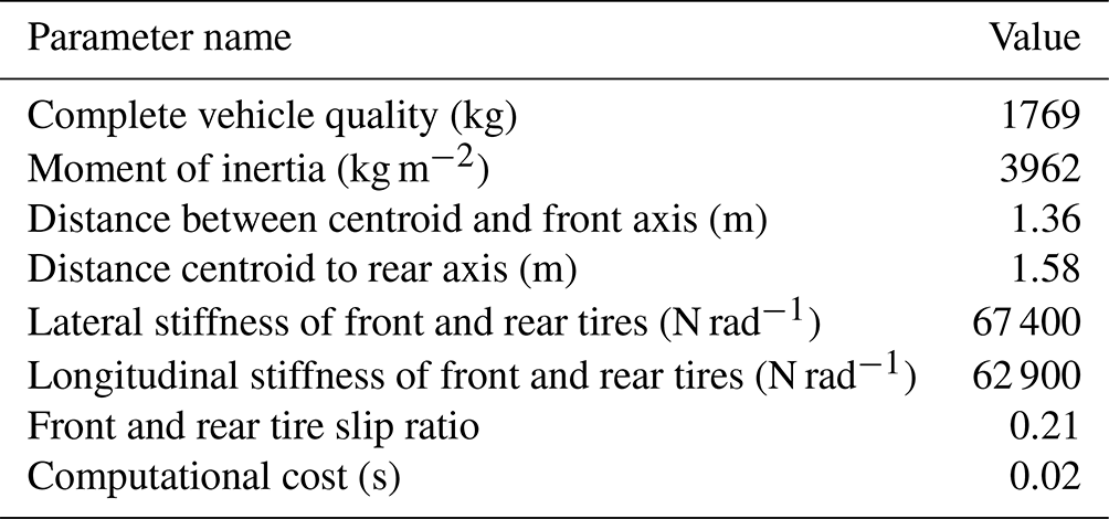
The CarSim and MATLAB/Simulink co-simulation is one of the mainstream simulation platforms in the current intelligent vehicle path-planning and path-tracking control test (Liang et al., 2020). CarSim and MATLAB/Simulink co-simulation results can be easily ported to real vehicles. At present, many scholars have applied the simulation results to the real vehicle. Firstly, the appropriate vehicle model is selected in CarSim, and the perception method used in this paper is the intelligent vehicle environment perception system of the CarSim software. The system includes vehicle sensors, cameras, and radar modules. The driving environment information obtained by the system is integrated to realize the understanding and recognition of the driving environment, and the driving environment that matches the real scene is constructed. Secondly, the corresponding program of the MPC algorithm is written by MATLAB. The vehicle model selected in CarSim and the program written by MATLAB are sent to Simulink. Finally, the selected vehicle model in CarSim, the built driving environment, and the program written by MATLAB are called by Simulink (Zhai et al., 2022). Vehicle stability and path-tracking accuracy are analyzed by Simulink. CarSim has a lot of accurate vehicle models to be chosen and can build accurate driving environments, but the program required for the MPC algorithm cannot be written in CarSim. The main function of MATLAB is to write the code needed for simulation, and MATLAB has a special interface to connect with CarSim. By Simulink, an accurate intelligent driving simulation module can be created. A lot of accurate vehicle models in CarSim and the driving environment close to the real scene make the simulation results more accurate. At the same time, the rich interfaces between CarSim and MATLAB/Simulink ensure that they can accurately simulate the effectiveness of the algorithm designed in this paper. Through CarSim and MATLAB/Simulink co-simulation, the path-tracking effects of different H_p at three fixed speeds were tested, and the relationship between the H_p and the speed was analyzed. Some parameters of the vehicle model involved in this simulation are shown in Table 1. Many vehicle models are available in CarSim software, and the software has verified the availability of the models through extensive experiments. The experiment was completed on a computer platform with an Intel Core i5-8400 CPU at 280 GHz (main frequency of 2.8 GH) and 8 GB memory. The vehicle model parameters used in this paper are provided by the public data set of the CarSim simulation software.

Table 1 Vehicle model parameters.

Simulation 1: the vehicle speed is set to 40 km h⁻¹. The prediction horizons are set to 6, 9, 12, and 15, respectively. Figure 5 shows the results of vehicle low-speed simulation.

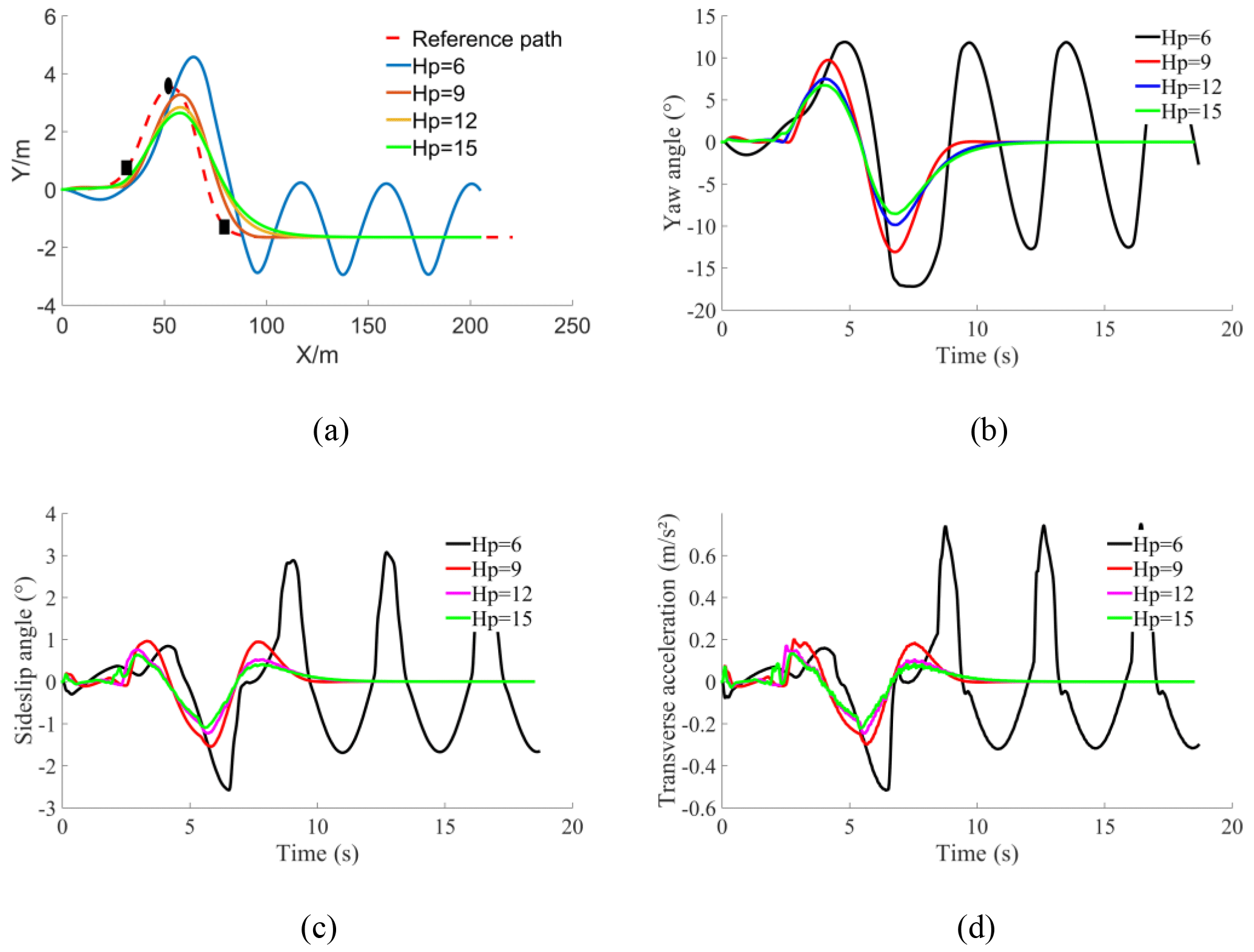
Figure 5 Vehicle low-speed simulation results. (a) Tracking path. (b) Yaw angle. (c) Sideslip angle. (d) Transverse acceleration.

Figure 5a shows that, when H_p=6, path tracking fails, and when H_p=9, path tracking is more accurate. Figure 5b and c are the results of the yaw angle and sideslip angle, respectively. The value of H_p is 9, and the error of the yaw angle and sideslip angle is the smallest. It can be seen from Fig. 5d that the lateral acceleration of the vehicle differs slightly, indicating that the vehicle has good stability at low speed.

Simulation 2: the vehicle speed is set to 70 km h⁻¹. The prediction horizons are set to 9, 12, and 15, respectively. The simulation results of mid-speed vehicles are given in Fig. 6.

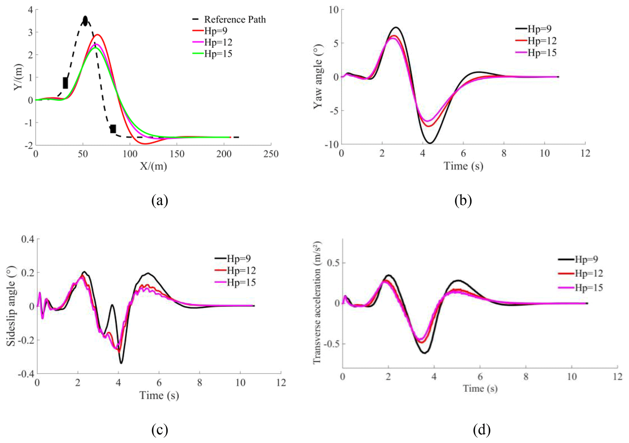
Figure 6 Vehicle mid-speed simulation results. (a) Tracking path. (b) Yaw angle. (c) Sideslip angle. (d) Transverse acceleration.

The path-tracking curve of Fig. 6a shows that, when H_p=12, the path-tracking accuracy is the highest. Figure 6b and c show that, when H_p=12, the yaw angle and the sideslip angle error are minimum, and when H_p=9, the error is maximum. It can be seen from Fig. 6d that, when H_p= 9, 12, and 15, the transverse acceleration of the vehicle is 0.61, 0.48, and 0.45 m s⁻², respectively. According to the engineering requirements of the Pacejka tire model (Pacejka and Bakker, 2007), when the transverse acceleration range of the vehicle is 0–3.92 m s⁻², the controller has good stability. Thus, the stability of the controller is judged by the smoothness and jitter of the lateral acceleration change. When H_p=12 and H_p=15, the change in the vehicle transverse acceleration curve is not smooth with jitter. When H_p=9, the transverse acceleration curve of the vehicle changes smoothly without obvious jitter, indicating that the controller has better stability when H_p=9.

Simulation 3: the vehicle speed is set to 100 km h⁻¹. The prediction horizon is set to 12, 15, and 18, respectively. Figure 7 is the simulation curve of the vehicle at high speed.

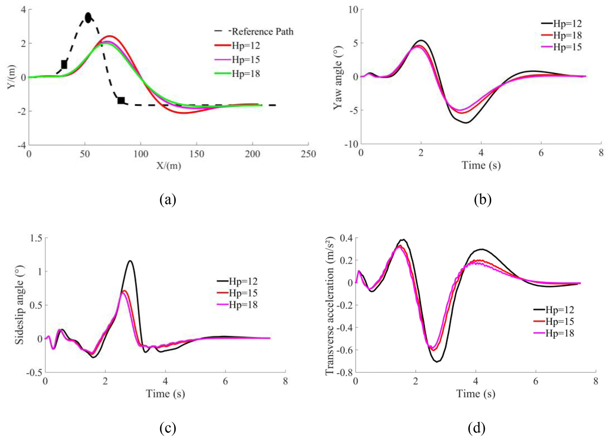
Figure 7 Vehicle high-speed simulation results. (a) Tracking path. (b) Yaw angle. (c) Sideslip angle. (d) Transverse acceleration.

Figure 7a shows that, when H_p=12 or 15, the path-tracking accuracy is not high, and when H_p=18, the path-tracking accuracy is the highest. Figure 7b and c show that, when H_p=15, the yaw angle and sideslip angle error is minimum. When the vehicle runs at high speed, the stability of the vehicle will be reduced.

5.2 Establishment of the speed–predictive horizon control law

Based on the analysis of Sect. 5.1, this paper performed a lot of simulations to explore the relationship between vehicle speed and prediction horizon. The relationship shows that there is an appropriate prediction horizon for the vehicle at a certain speed, which minimizes the path-tracking deviation of the vehicle. When other parameters remain unchanged, the relationship between speed and prediction horizon is approximately linear. According to the relationship, this paper uses a multiple fitting polynomial to calculate the optimal prediction horizon corresponding to different vehicle speeds.

When the vehicle detects the obstacles, the vehicle slows down, and the obstacle avoidance planning controller adjusts the prediction horizon in real time by the relationship between speed and prediction horizon (Wang et al., 2021; Chen et al., 2020). The expression of the speed–predictive horizon by two-times polynomial fitting for the adaptive obstacle avoidance planning controller is

$$\begin{array}{}\text{(20)}& \begin{array}{rl}& H_{{\mathrm{p}}_{\mathrm{1}}}\\ & =\left\{\begin{array}{l}\mathrm{8},v\le \mathrm{30}\\ \text{int}\left(\mathrm{0.0025}{v}^{\mathrm{2}}-\mathrm{0.0529}v+\mathrm{8}\right),\mathrm{30}<v<\mathrm{100}\\ \mathrm{18},v\ge \mathrm{100}\end{array}\right.,\end{array}\end{array}$$

where v is the vehicle speed, int is the full character, and $H_{{\mathrm{p}}_{\mathrm{1}}}$ is the predictive horizon of the obstacle avoidance planning controller.

As shown in Fig. 8, the predictive horizon of the obstacle avoidance planning controller evolution diagram is given.

Figure 8 Predicted horizon evolution diagram.

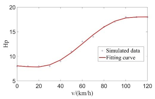
When the vehicle is driving on a road without obstacles, the vehicle will travel according to the reference path. At this time, the change in vehicle speed will also affect the prediction horizon in the path-tracking controller. Similarly, the expression of the speed–predictive horizon by three-times polynomial fitting for the adaptive path-tracking controller is

$$\begin{array}{}\text{(21)}& \begin{array}{rl}& H_{{\mathrm{p}}_{\mathrm{2}}}\\ & =\left\{\begin{array}{l}\mathrm{8},v\le \mathrm{30}\\ \begin{array}{rl}& \text{int}(-\mathrm{0.000042866}{v}^{\mathrm{3}}+\mathrm{0.0116}{v}^{\mathrm{2}}-\mathrm{0.6944}v\\ & +\mathrm{20}),\mathrm{30}<v<\mathrm{100}\end{array}\\ \mathrm{20},v\ge \mathrm{100}\end{array}\right.,\end{array}\end{array}$$

where $H_{{\mathrm{p}}_{\mathrm{2}}}$ is the predictive horizon in the path-tracking controller.

5.3 Convergence analysis of the algorithm

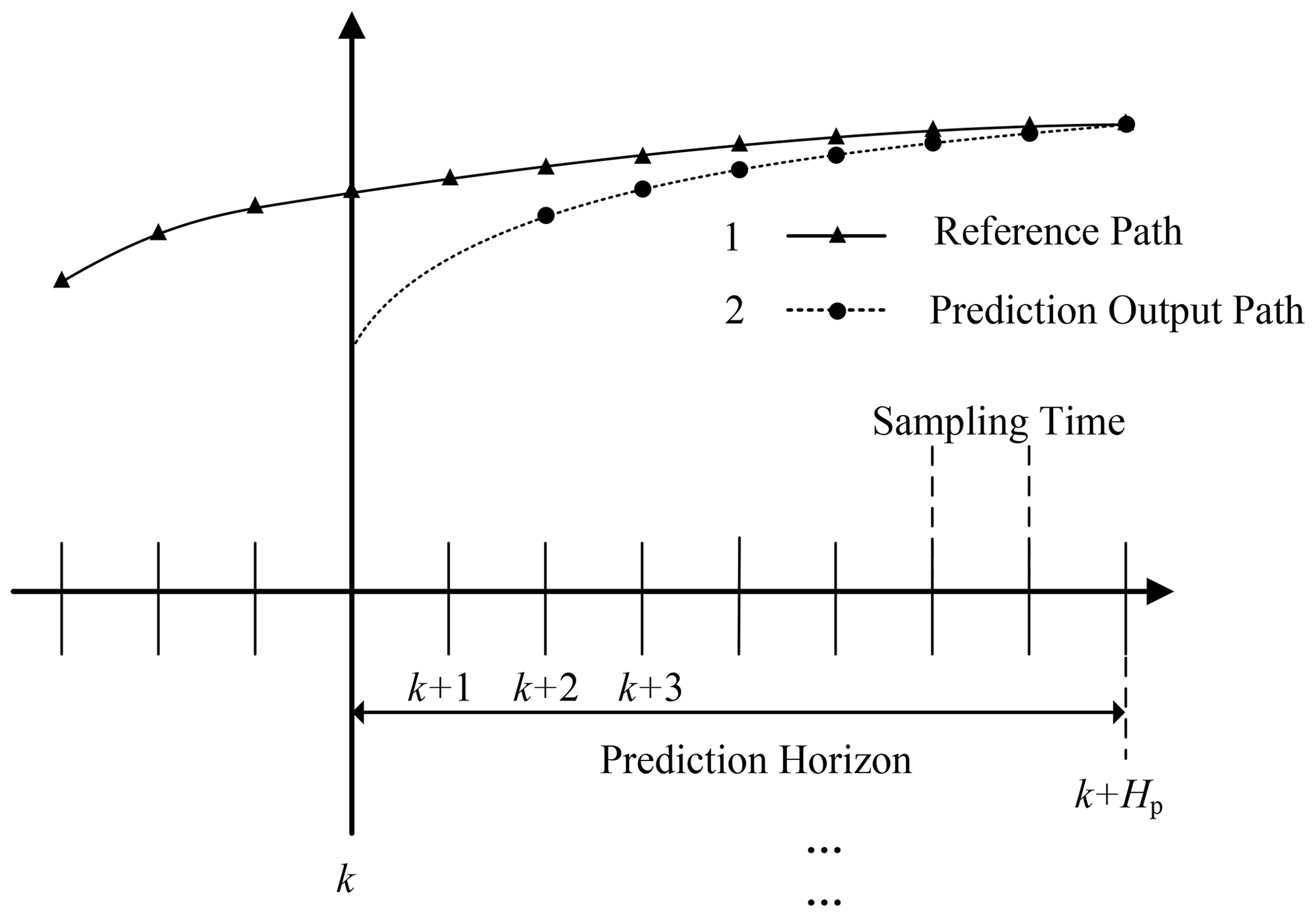
The convergence analysis of the algorithm can be illustrated by Fig. 9 (Taghavifar and Rakheja, 2019). In the whole control process, suppose the current time is k, and curve 1 is the reference path. Curve 2 represents the predicted output path of the controller, and to meet the requirements of path-tracking control, curve 2 should coincide with curve 1 as much as possible. It can be seen from curve 2 that the predicted output path is gradually close to the reference path.

Figure 9 Convergence analysis of the algorithm.

6 Simulation analysis

The Sect. 5.1 analysis shows that the traditional model predictive controller with constraint conditions can safely and stably track the reference path and avoid obstacles on the road under different vehicle speeds (low speed 40 km h⁻¹, medium speed 70 km h⁻¹, and high speed 100 km h⁻¹). The vehicle tracking accuracy and controller stability are analyzed under different vehicle speeds and different H_p values. On the basis of adding constraints, combined with the speed–predictive horizon control law, a double-layer adaptive MPC (AMPC) path-tracking controller is constructed. The control effect of the path-tracking controller under variable speed conditions is analyzed. The double-layer AMPC is compared with the traditional MPC and the single-layer AMPC (speed–predictive horizon control law only established in the obstacle avoidance planning layer). The variable speed condition is built in CarSim. In order to improve the calculation speed and control precision of the controller, the simulation is carried out in a single obstacle environment. The simulation results are shown in Fig. 10.

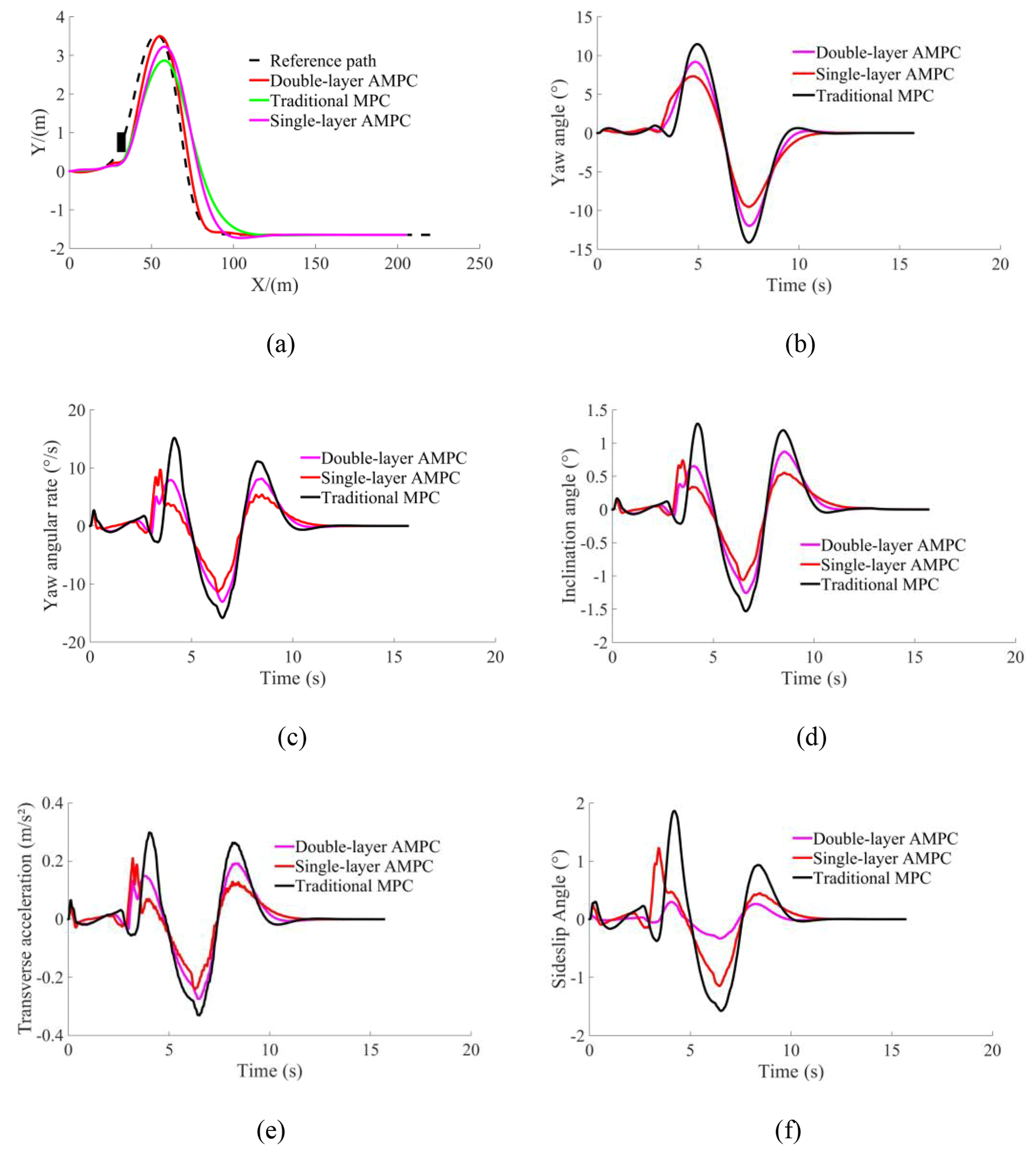
Figure 10 Comparison of simulation results. (a) Tracking path. (b) Yaw angle. (c) Yaw angular rate. (d) Inclination angle. (e) Transverse acceleration. (f) Sideslip angle.

The accuracy of path tracking can be expressed by the lateral deviation between the actual trajectory of the vehicle and the planned one. The smaller the lateral deviation, the higher the path-tracking accuracy. Figure 10a can reflect the vehicle path-tracking accuracy. It can be seen that the maximum lateral deviation of the double-layer adaptive MPC controller is 0.12 m, the maximum lateral deviation of the single-layer adaptive MPC controller is 0.37 m, and the maximum lateral deviation of the traditional MPC controller is 0.63 m. Compared with the algorithm proposed by Dai et al. (2020), the maximum lateral error of the proposed algorithm is reduced by 0.09 m. The deviation of double-layer adaptive MPC controller is minimal, and thus the double-layer adaptive MPC has the highest tracking accuracy. In terms of vehicle driving stability, Fig. 10b and c show that the error of the yaw angle of the double-layer adaptive MPC vehicle is the smallest. From Fig. 10c, it can be seen that the fluctuation range of the yaw angular rate of the control algorithm proposed in this paper is 21.20 degree s⁻¹, the fluctuation range of the yaw angular rate of the single-layer adaptive MPC controller is 21.14 degree s⁻¹, and the fluctuation range of the yaw angular rate of the traditional MPC controller is 31.02 degree s⁻¹. The results show that the fluctuation range of the yaw angular rate of the control algorithm proposed in this paper is small and has no obvious jitter, indicating that the control algorithm proposed in this paper has good stability. In general, inclination angle and transverse acceleration are the indexes used to evaluate vehicle comfort (Xu et al., 2021). Simulation results in Fig. 10d and e show that the maximum inclination angle of the traditional MPC vehicle is 1.53^∘, the maximum inclination angle of the double-layer adaptive MPC vehicle is 1.25^∘, the maximum transverse acceleration of the traditional MPC is 0.34 m s⁻², and the maximum transverse acceleration of the double-layer adaptive MPC is 0.27 m s⁻². It can be seen from Fig. 10f that the fluctuation range of the sideslip angle of the control algorithm proposed in this paper is 0.30^∘, the fluctuation range of the sideslip angle of the single-layer adaptive MPC controller is 1.23^∘, and the fluctuation range of the sideslip angle of the traditional MPC controller is 1.87^∘. Compared with the algorithm proposed by Xie et al. (2021), the improved algorithm in this paper shows a smaller fluctuation range of the vehicle sideslip angle, indicating that the driving stability of intelligent vehicles is better. The results show that the fluctuation range of the sideslip angle of the control algorithm proposed in this paper is the smallest, indicating that the control algorithm proposed in this paper has good stability. Combined with the analysis of the simulation results, the proposed double-layer adaptive MPC control strategy not only has the highest path-tracking control accuracy, but also has good safety and stability.

7 Conclusion

In this paper, a double-layer adaptive model predictive controller is designed. In the obstacle avoidance planning controller, the vehicle point mass model is used to expand the obstacle, and the safe collision distance model is established according to the relationship between obstacle and vehicle position. In the path-tracking controller, the vehicle dynamics model is adopted. Based on the model predictive control algorithm, the vehicle sideslip angle and acceleration constraints are added to transform the path-tracking control into a quadratic programming problem with constraints. The CarSim and MATLAB/Simulink simulation results show that the double-layer adaptive model predictive controller designed in this paper can effectively improve the path-tracking accuracy, safety, and stability of intelligent vehicles.