the Creative Commons Attribution 4.0 License.
the Creative Commons Attribution 4.0 License.
 | 05 May 2023
Topology optimization for thermal structures considering design-dependent convection boundaries based on the bidirectional evolutionary structural optimization method
Yanding Guo
Dong Wei
Tieqiang Gang
Xining Lai
Xiaofeng Yang
Guangming Xiao
Lijie Chen
Based on the bidirectional evolutionary structural optimization (BESO) method, the present article proposes an optimization method for a thermal structure involving design-dependent convective boundaries. Because the BESO method is incapable of keeping track of convection boundaries, virtual elements are introduced to assist in identifying the convection boundaries of the structure. In order to solve the difficult issue of element assignment under a design-dependent convection boundary, label matrixes are employed to modify the heat transfer matrix and the equivalent temperature load vector of elements over topology iterations. Additionally, the optimization objective is set to minimize the maximum temperature of the structure in order to deal with the objective reasonableness, and the p-norm method is then used to fit the objective function to calculate sensitivity. Finally, several cases, including 2D and 3D structures under various heat transfer boundary conditions, are provided to illustrate the effectiveness and good convergence of the proposed method.
- Article
(5551 KB) - Full-text XML
- BibTeX
- EndNote


Structural topology optimization, as an effective method of structural weight reduction, has been paid more and more attention in recent years. However, a lightweight design for a thermal structure under various boundary conditions still faces great challenges (Deaton and Grandhi, 2015; Zhu et al., 2015), namely because studies under first-type (Dirichlet boundary) and second-type (Neumann boundary) boundary conditions are more common than those under convection (Robin boundary) boundary conditions (Zhou et al., 2016).
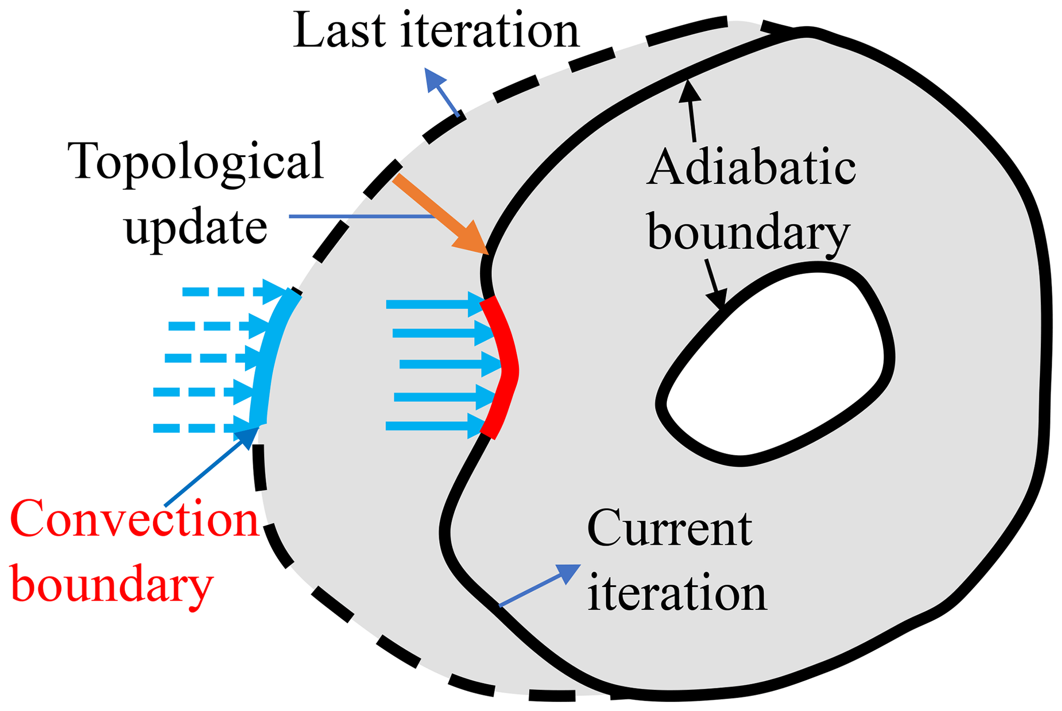
Previous topology optimization of thermal structure considering the Robin (third-type) boundary (i.e., the convection boundary) has mostly been founded on density-based and level set methods. In density-based optimizations, it is necessary to create explicit boundaries by setting a cutoff value for elements' density; some classical manners to do this have been proposed, including the following: the hat function (Iga et al., 2009; Dede et al., 2015), the peak interpolation method (Yin and Ananthasuresh, 2001), the element connection parameter method (Ho Yoon and Young Kim, 2005) and convection interpolation (Bruns, 2007; Alexandersen, 2011). However, the choice of the truncation value of the above methods depends heavily on the experience of the designer, and an inappropriate cutoff value may result in ill-defined boundaries, such as “islands” (i.e., isolated solid materials). Some studies have been based on the explicit bounds of the level set method in order to realize the implementation of convection boundaries (Ahn and Cho, 2010; Coffin and Maute, 2015; Li et al., 2022). However, the level set method has the disadvantage of initialization dependence; thus, the location of convection boundaries will greatly affect the optimization results. More importantly, the above studies did not consider the fact that a structure boundary might be partly convective (Hu et al., 2008; Wang and Qian, 2020; Yan et al., 2021). Hence, it is necessary to identify whether a boundary is convective, adiabatic or partly convective. However, the difficulty here is that the solid or fluid region is updated during the iterations. As a result, the convection boundary changes with the iteratively altered structural boundary, as shown in Fig. 1.
Bidirectional evolutionary structural optimization (BESO) methods are also one of the main methods for topology optimization. They have the advantage of good convergence and initialization independence (Radman, 2021) and have been widely used in structural heat transfer (Xia et al., 2018), frequency (Gan and Wang, 2021), acoustics (Pereira et al., 2022) and material microstructure optimization design (Qiao et al., 2019), among others. In addition, BESO-type methods can provide a clear, explicit boundary (Da et al., 2018), which has been employed to solve the transmissible load problem (Fuchs and Moses, 2000; Yang et al., 2005) and the pressure load problem (Picelli et al., 2015, 2017). However, according to the heat transfer equation, the convective boundary is more complex than the transmissible or pressure load, as the convective boundary affects not only the equivalent temperature load but also the heat transfer capacity of the structure itself. Therefore, the current BESO method needs to be further investigated with respect to the design-dependent convection boundary in order to improve its applications to more complicated boundary conditions.
This article is devoted to the topological optimization of thermal structures considering the design-dependent convection boundary based on the BESO method. The remainder of the paper is structured as follows: in Sect. 2, the difficulties involved with thermal topology optimization considering the convection boundary are outlined; in Sect. 3, the corresponding solution method is proposed, including the identification of the convection boundary and the assignment of the convection matrix; in Sect. 4, the selection of the topology optimization objective is discussed, and the corresponding sensitivity is analyzed; and, finally, in Sect. 5, numerical cases with various boundary conditions are analyzed to verify the effectiveness and good convergence of the proposed method.
For the heat transfer problem, there are three types of thermal boundary conditions (Palani and Ganesan, 2007): the first-type boundary (S1), called the Dirichlet condition, corresponds to a given fixed temperature on the system; the second-type boundary (S2), namely the Neumann condition, corresponds to a given heat flux on the boundary; and the third-type boundary (S3), the Robin condition, corresponds to a given convection coefficient and the ambient temperature on the boundary. These boundary conditions can be expressed as follows:
Here, is temperature given on S1, qT is the nodal temperature of the structure and T∞ is the ambient temperature. , and represent the thermal conductivity in the respective x, y and z directions. nx, ny and nz are the cosine of the normal line outside the boundary. is the given heat flux on S2, and is the convection coefficient on S3.
When the boundary conditions are satisfied, the steady-state heat equation of discrete elements is obtained using the finite element method (FEM):
where is the element heat transfer matrix, is the temperature vector of element nodes and is the equivalent temperature load vector of element nodes. The specific forms of and are as follows:
Here, N is the shape function matrix. It should be noted that the internal heat source intensity is not considered in this article.
According to Eq. (3), the first term on the right of the equation represents the contribution of conductivity, and the second term represents the contribution of convection. According to Eq. (4), the first and the second terms on the right of the equation reflect the equivalent temperature load generated by given heat flow and given convection, respectively. Further, Eqs. (3) and (4) can be expressed as follows:
Here,
In the above expressions, is the elemental heat transfer matrix of thermal conductivity, is the identity matrix form of , is the thermal conductivity, is the element equivalent temperature load, is the element equivalent temperature load of the heat flux, is the element heat transfer matrix of convection, is the identity matrix form of , is the element equivalent temperature load of convection and is the identity vector form of .
Moreover, the element heat transfer matrix and the equivalent temperature load vector of element nodes are assembled using the FEM to form the heat transfer matrix and the temperature load vector of structure nodes:
where KT is the heat transfer matrix, is the heat transfer matrix without convection, HT is the convection heat transfer matrix, PT is the equivalent temperature load vector, Pf is the equivalent temperature load generated from the heat flux and Ph the equivalent temperature load generated by convection. When convection is excluded, Ph=0.
In the BESO method, when the value of topological variables is 1, the corresponding elements are solid elements (SEs); when the value is a small quantity, such as 0.001 (not 0 to avoid singularity), the corresponding elements are nonsolid elements with very poor properties (Huang and Xie, 2010). If the design-dependent convection boundary is considered, the boundaries can be classified into two types: convective boundaries and adiabatic boundaries. Therefore, in this article, the nonsolid elements should be further subclassified into fluid elements (FEs) and void elements (VEs). As a result, the convection boundary can be identified from the interfaces between the SEs and the connected FEs (Deshmukh and Warkhedkar, 2013; Chamkha et al., 2017).
However, due to the variation in the FEs, the VEs and the SEs with optimization iteration, it is necessary to take measures to keep track of the iteratively changed convection boundary. Additionally, according to Eq. (10), the assignment of KT and PT also needs extra treatments.
This section is dedicated to realizing the identification of the convection boundary in the design domain during the iteration processes (in Sect. 3.1) and to assigning the corresponding convection contribution matrix (in Sect. 3.2).
3.1 Identification of the convection boundaries
In 2D structures, convection can be classified into two categories: (1) top and bottom convection (TBC), in which the direction is vertical to the structure surface, and (2) side convection (SC), in which the direction is parallel to the structure surface (Alexandersen, 2011). In the TBC case, all sides of an element will be influenced by convection, and the structural boundaries in such problems are all convective. In the SC case, convection affects partial sides of an element, and it is necessary to further confirm whether a boundary of the element is convective. Compared with the optimal design under TBC, the optimal design under BC requires an extra scheme to identify convective boundaries (rather than merely based on the geometry boundary); therefore, the latter design it is more complex and will be investigated in this article. In 3D structures, there is only one type of convection; it is similar to SC in 2D structures, but the difference is that the convection affects partial planes of an element. Hence, the convection boundary identification method for SC proposed later in this article can be applied to both 2D and 3D structures.
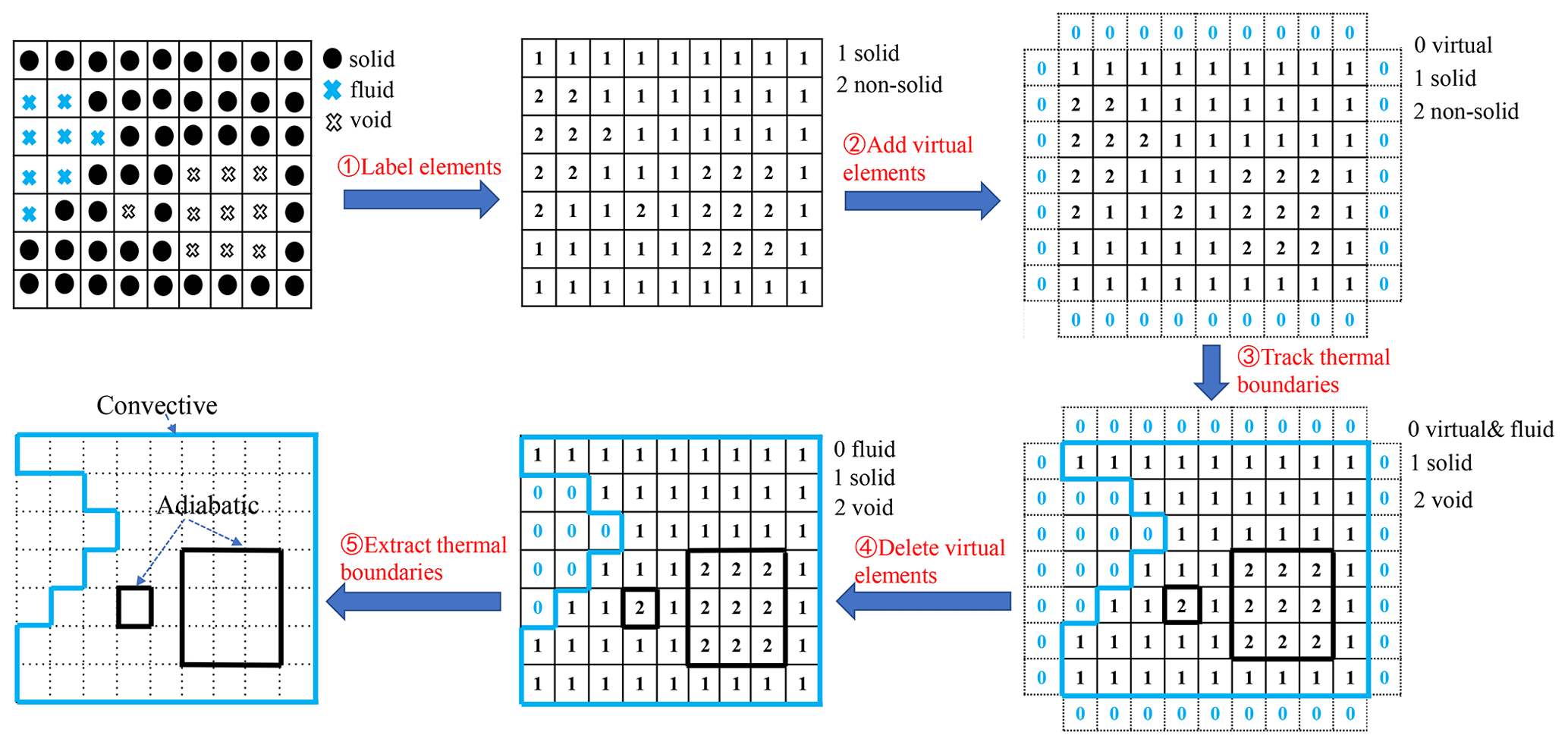
As the BESO method cannot keep track of convective boundaries (Qiao et al., 2019), virtual elements are introduced in this article in order to distinguish FEs from nonsolid elements. Using convection acting on the surface of a 2D structure as an example, a schematic diagram is shown in Fig. 2 that outlines the following specific steps:
- i.
In the design domain, the identifier of the solid elements is labeled “1” and that of the nonsolid elements is labeled “2”.
- ii.
A layer of virtual elements around the design domain are added, and their identifier is marked as “0”. It is noted that these virtual elements do not participate in FEM calculations.
- iii.
All elements are then “traversed”. If the identifier of an element is 2 and the identifier of any adjacent element is simultaneously 0, the identifier is changed to 0; if this is not the case, the identifier remains at its original value. To ensure identification, it is necessary to carry out this process enough times. The number of times that this process is carried out is related to the number of elements with an initial identifier of 2. As there is the possibility that only the last element of the traversal is marked as 0 and that the identifiers of all the preceding elements are 2, we can only guarantee the validity of the element identifier conversion by ensuring that the minimum number of iterations is the same as the number of initial elements marked as 2.
- iv.
All of the virtual elements are deleted. The remaining elements with an identifier value of 2, 1 and 0 are void elements, fluid elements and solid elements, respectively.
In each topology iteration, steps (i)–(iv) are repeated to distinguish the FEs and VEs. The corresponding physical convection boundaries then exist at the interfaces between SEs and FEs.
3.2 Assignment of the convection matrixes
After the identification of the convection boundary of solid elements, it is necessary to further modify the element heat transfer matrix and temperature load vector influenced by convection.
Because convection only affects part of the boundary of the element, this paper introduces label matrixes to achieve the assignment of the matrixes related to convection. There are two parameters that affect convection: the convection coefficient and the ambient temperature. The label matrix of the convection coefficient is denoted as the G matrix. The label matrix of ambient temperature is denoted as the M matrix. In this article, the elements used in 2D structure are quadrilateral elements, and the elements used in 3D structure are hexahedral elements. Therefore, the number of elements of G matrix and M matrix in 2D and 3D structures is 4 and 6, respectively:
Here, n=4 in a 2D structure and n=6 in a 3D structure.
If a component (such as G1) of matrix G or M is marked as 1, the convection and the ambient temperature are taken into account for an element boundary. On the contrary, 0 means that the convection and the ambient temperature are not considered for an element boundary. Accordingly, employing the G and M matrixes, Eqs. (8) and (9) can be rewritten as follows:
Here, Γ is the element boundary.
For the reader's understanding, using the convection acting on the surface of a 2D structure as an example, the steps related to the assignment of the convection matrix to elements by label matrixes are summarized as follows:
- i.
If an element is nonsolid element (its identifier is 0 or 2), the G and M matrix of this element is a 0 matrix. If it is a solid element, go to the next step.
- ii.
Check the identifier of its neighboring elements counterclockwise from the left edge, and then fill the G and M matrixes with 0 or 1 in turn.
- iii.
The element heat transfer matrix and the element temperature load vector considering convection are obtained by Eqs. (12) and (13).
Due to the design dependence of convective boundaries, steps (i)–(iii) need to be repeated in each iteration.
4.1 Selection of the optimization objective
In the BESO method, the objective function and constraints of optimization are expressed as follows:
Here, Ob is the optimization objective, Ve is the volume of each element, x is the topological variable and xi is the topological variable of element. For more details on the framework of the BESO method, the reader is referred to Huang and Xie (2008).
The optimization objective in this article is exclusively involved with the thermal field. It is initially assumed that the temperature field and load are related to topological variables; thus, the objective function depends on the temperature field, temperature load and topological variables, namely
As the gradient of the node temperature with respect to the element topology variable is solved as an implicit function, a Lagrangian multiplier is introduced in order to eliminate this term (Deb and Srivastava, 2012; Wah et al., 2000):
For this problem, the gradient of the objective function can be obtained:
In previous works, the optimization goal has usually been set to minimize the thermal compliance of the structure (Picelli et al., 2017; Zhou and Li, 2008) – that is, Ob=PTqT. This is because, under a fixed heat flow, minimizing the objective function is equal to maximizing the structural heat transfer matrix, namely
However, according to Eqs. (12) and (13), the existence of convection boundaries means that the structure has both a design-dependent heat transfer matrix and nonconstant external load. According to Eq. (18), minimizing the thermal compliance cannot guarantee that the maximum thermal conduction capability is obtained. Thus, the effectiveness of the objective function in Eq. (18) is open to discussion under a design-dependent convection boundary.
In the present article, the optimization objective is set to minimize the maximum temperature in the structural temperature field, which can directly reflect the thermal conduction capability of structures. However, the maximum temperature is a scalar with no gradient. Thus, the p-norm method (Zhai et al., 2018) with a gradient is used to fit the maximum temperature. The objective function can be expressed as follows:
where LT is a unit vector used to calculate the summation and p is the value of the norm. In order to illustrate the advantages of minimizing the maximum temperature as an objective function in topology optimization considering design-dependent convection boundaries, a comparison of the topological results with the maximum temperature and the thermal compliance as the respective objective functions is made in Sect. 5.
4.2 Sensitivity analysis
For the BESO method, sensitivity determines the “birth and death” of elements (Xu et al., 2020), which can be solved by the gradient of the objective function (Huang and Xie, 2009). From Eq. (17), the corresponding Lagrangian adjoint matrix of the objective function is
Denoting , the general equation of sensitivity is
The material interpolation model adopted in this article is the Solid Isotropic Material with Penalization (SIMP) model (Tavakoli and Davami, 2008). Then, compared with the sensitivity without considering design-dependent convection and the sensitivity of thermal compliance (), the sensitivity considering design-dependent convection can be obtained as follows:
where pe is the power law of the penalty. In Eq. (22), the right side of the equation consists of three parts that represent the sensitivity of the heat transfer coefficient, the convection matrix and the equivalent temperature load vector to the objective function, respectively. The detailed derivation process is presented in Appendix A.
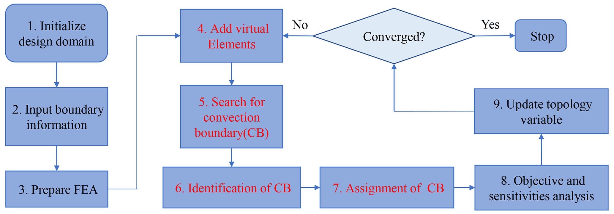
Based on the work in Sects. 3 and 4, some typical cases of thermal structures with convective boundary conditions are analyzed in this section, and the topological optimization flowchart is shown in Fig. 3.
The convection boundary condition, also known as the mixed boundary, can be combined with both the first-type boundary and the second-type boundary to solve the temperature field. In order to illustrate all of the types of structural optimization designs under convection conditions, topological optimization problems considering combination boundary conditions including design-dependent convection boundaries are classified into three categories:
-
structural optimization under a combination of convection boundaries and the first-type boundary conditions, i.e., the S13 problem;
-
structural optimization under a combination of convection boundaries and the second-type boundary conditions, i.e., the S23 problem;
-
structural optimization under a combination of convection boundary, first-type boundary and second-type boundary conditions, i.e., the S123 problem. The S123 problem is a hybrid of the S13 problem and the S23 problem.
In addition, it should be noted that convection, including forced convection and natural convection, is a complex boundary condition. The convection coefficient is influenced by the velocity and properties of the fluid as well as by the shape and properties of solid structures (Yang et al., 2013). Although the convection coefficient maybe varies, a constant convection coefficient is specified during topology iterations, as this article mainly focuses on the method of topology optimization for a thermal structure. The materials properties and topology parameters are listed in Table 1.
Table 1Parameters for the numerical calculations.
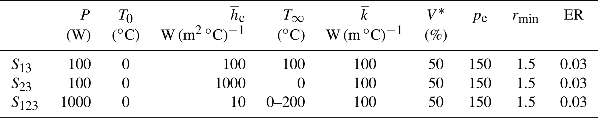
Note that “rmin” denotes the filter radius and “ER” represents the evolutionary rate. Detailed information on rmin and ER are given in Huang and Xie (2010).
5.1 The S13 problem
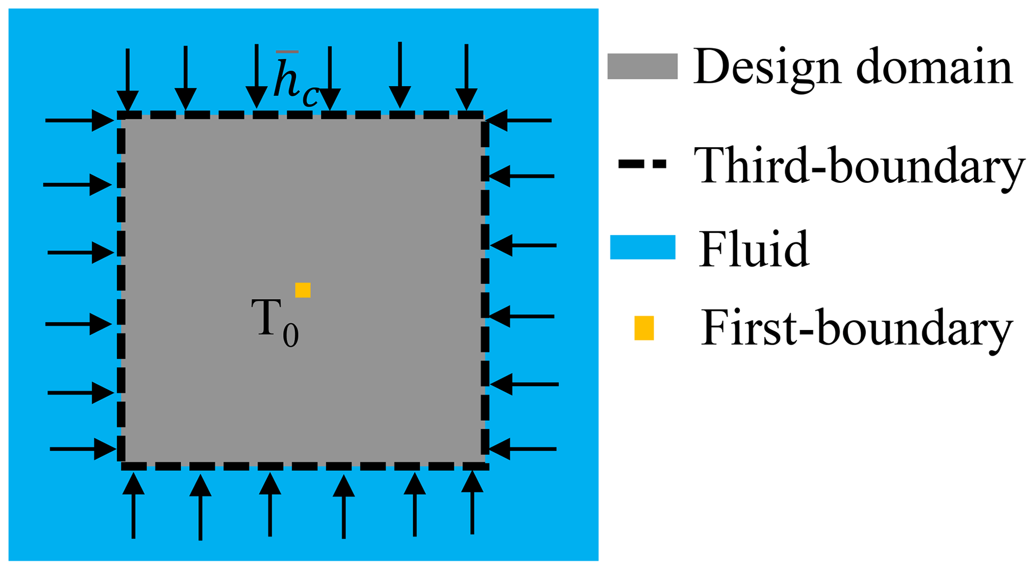
In this subsection, the thermal structure optimization results under a combination boundary conditions including convection and the temperature constraint are discussed. The design domain is a 0.5 m × 0.5 m flat plate with a thickness of 1 cm, and the number of elements is 50×50. The first boundary condition is applied to the geometric center of the design domain. The convective fluid elements are distributed around the design domain, and the newly generated cavities within the structure during topology optimization have no fluids and are adiabatic boundaries. The initial conditions are shown in Fig. 4.
In this case, as the ambient temperature (100 ∘C) is higher than the structure temperature (0 ∘C), the convection boundaries mainly provide the equivalent temperature loads to the structure. With the optimization iterations, the optimal processes based on the present proposed method with the maximum temperature as the objective function and the thermal compliance as the objective function are presented in Fig. 5a and b, respectively.
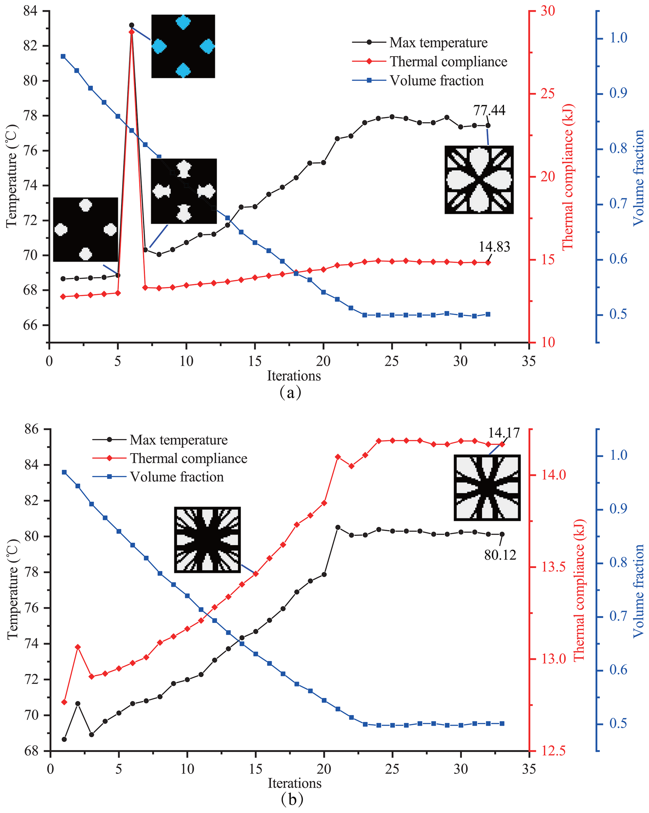
Figure 5Optimal process for the S13 problem for different optimization objectives: (a) optimization objective of maximum temperature and (b) optimization objective of thermal compliance.
From Fig. 5a and b, with the iteration proceeding, it can be seen that the value of the objective function increases, which is a typical characteristic of BESO (Huang and Xie, 2008). The final maximum temperature and thermal compliance reached based on the proposed method with the maximum temperature as the objective function are 77.44 ∘C and 14.83 kJ, respectively, as shown in Fig. 5a. Comparably, the final maximum temperature and thermal compliance reached with thermal compliance as the objective function are 80.12 ∘C and 14.17 kJ, respectively, as shown in Fig. 5b. These results obtained with the two optimization objectives are very close, which is due to the fact that the final boundaries of convection in this case are the same as the initial boundaries, thereby satisfying the condition of a constant convection boundary in Eq. (18), and taking the thermal compliance as the optimization objective is still valid. However, using the maximum temperature as the optimization objective is still meaningful because the maximum temperature of the optimized configuration for this objective is lower.
Additional numerical instability appeared in iteration 5–7 in Fig. 5a, which was caused by the increase in the convection area. As seen in Fig. 6, in iteration 5, the generated topological cavities are disconnected with the outer surface of the structure, and convection only acts on the same part on the surface as that under the initial conditions. However, in iteration 6, the inner cavities propagate to connect with the outer surface, resulting in the convection areas extending to the boundary of the cavities. The increase in the convection area means that convection provides more heat to the structure, leading to a rise in the temperature of the structure. For this problem, the proposed optimization method in the present article, based on the BESO strategy, can correct the inappropriate element elimination according to the sensitivity information. In the following iteration 7, the internal cavity boundaries are modified to disconnect from the external surface, and the optimization iterations appear stable. The resulting configuration and corresponding temperature field are shown in Fig. 7.
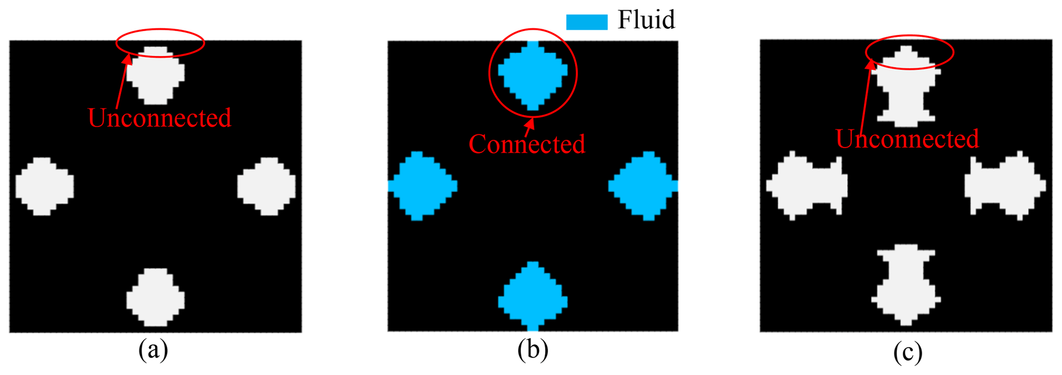
Figure 6Connectivity between the internal cavities and the outer surface of the structure in iterations 5 to 7: (a) iteration 5, (b) iteration 6 and (c) iteration 7.
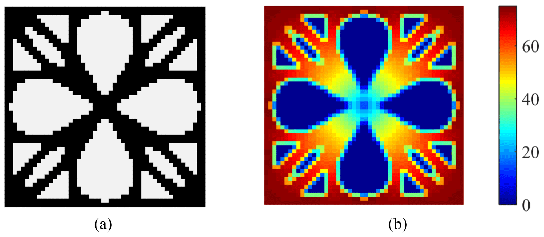
Figure 7(a) Final topology configuration and (b) the corresponding temperature field of elements (obtained by averaging the temperature of element nodes).
In Fig. 7a, the outer surface (convection areas) of the structure remains unchanged, which is reasonable to reduce the convection areas (as mentioned earlier). A similar phenomenon was also pointed out by Wang and Qian (2020). Furthermore, the boundaries of the internal cavities are adiabatic, and the temperature in the cavities' body is 0 ∘C, as shown in Fig. 7b. Compared with the S12 problem (convection boundary replaced by thermal flux, as shown in Fig. 8a), the similarity of the topological iteration curves (as shown in Fig. 8b) and the final configuration (as shown in Fig. 8c) illustrates that the essence of the convection boundary under the S13 condition is to provide heat to the structure. Moreover, the convergence of the proposed method (32 iterations) is comparable to that of the traditional BESO method (36 iterations).
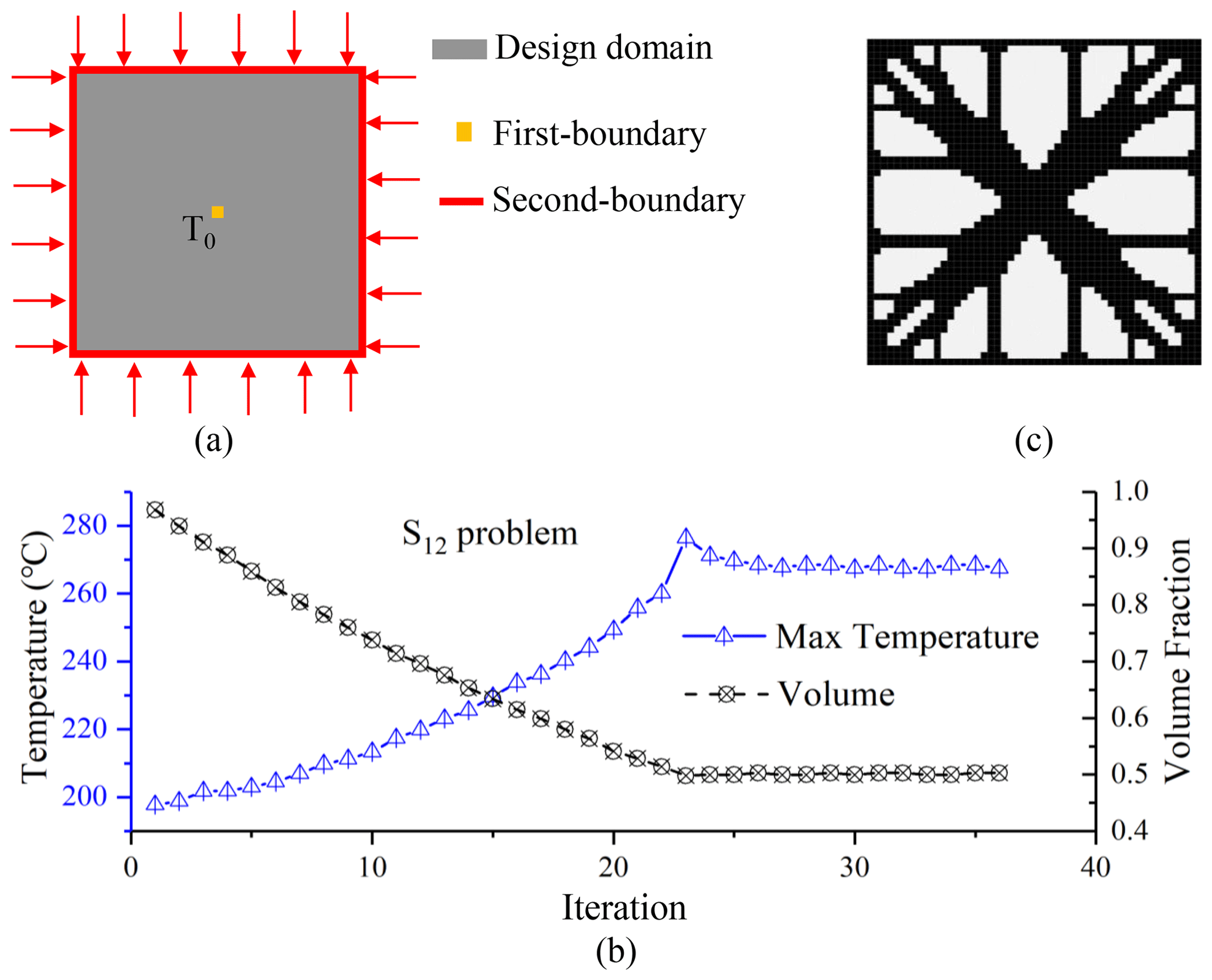
Figure 8Initial conditions and optimization results for the S12 problem: (a) initial condition for the S12 problem; (b) optimal process for the S12 problem; (c) final configuration for the S12 problem.
5.2 The S23 problem
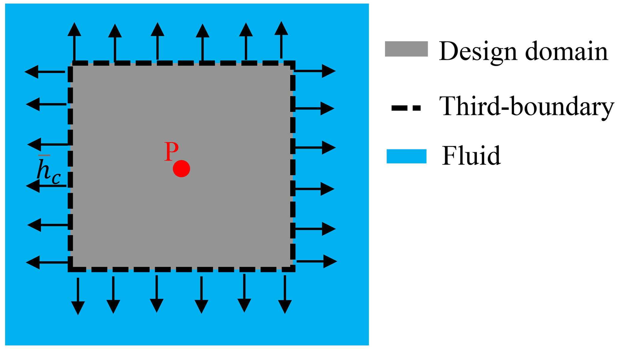
In this subsection, the optimization of the thermal structure under a combination of boundary conditions including the convection boundary and the heat flux is discussed. For the initial structure, there is an equivalent temperature load P in the center and periphery convection boundaries; other conditions are the same as the case in Sect. 5.1, as shown in Fig. 9.
In this case, as the ambient temperature (0 ∘C) is lower than the structure temperature with a heat source (P=100 W) in the central structure, the convection boundary is to functionally dissipate heat. The optimal iterative processes and the structural evolution using the proposed method with the maximum temperature as the objective function and the thermal compliance as the objective function are shown in Fig. 10a and b, respectively.

Figure 10Optimal process for the S23 problem for different optimization objectives: (a) optimization objective of maximum temperature and (b) optimization objective of thermal compliance.
From Fig. 10a, when taking the maximum temperature as the objective function, the distance between the convective boundary and the heat source becomes closer and closer with proceeding iterations (as shown in Fig. 11), which results in a reduction in the initial structural maximum temperature (92.62 ∘C) to the final value of 88.42 ∘C, and the corresponding thermal compliance decreases from 9.26 to 8.84 kJ.
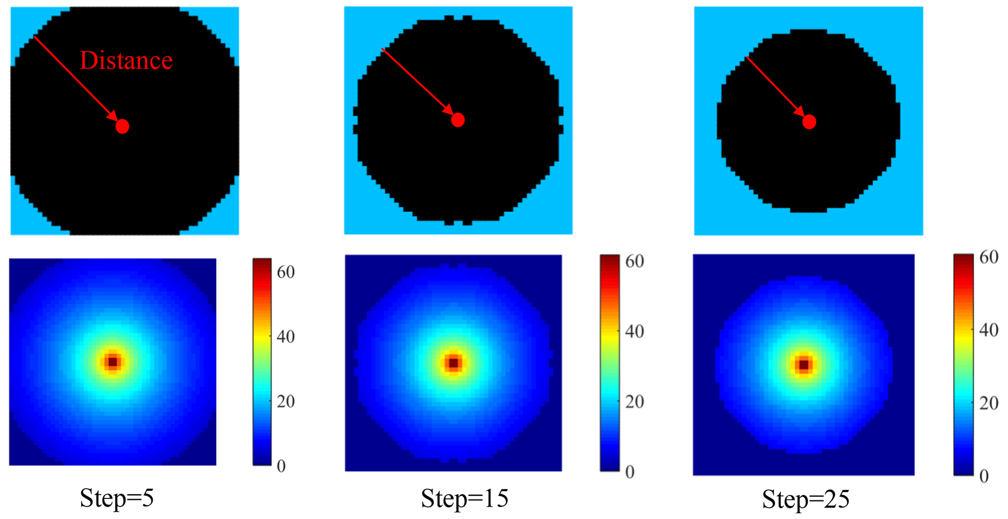
Figure 11The change in distance between the convection boundary and the heat source (getting closer and closer) as well as the change in the corresponding structural temperature field (based on the average temperature of element nodes) with proceeding iterations.
However, as shown in Fig. 10b, when taking thermal compliance as the optimization objective, the iterative curve continues to oscillate during the volume fraction reduction phase (iterations 1–23). When the volume fraction reaches the target value (iterations 23–68), the overall variation trends in the maximum temperature and thermal compliance of the configuration both increase with proceeding iterations. Finally, the final maximum temperature converges to 98.35 ∘C, which is 5.73 ∘C higher than the initial value. The corresponding final thermal compliance converges to 9.84 kJ, which is a 0.54 kJ increase compared with the initial value. This is due to the fact that the convective boundaries are changing iteratively in this case, which no longer satisfies the condition of constant convective boundaries in Eq. (18), causing the minimum of the thermal compliance not to equal the maximum of the heat transfer capability and, thus, an unreasonable final configuration. In contrast, it is obvious that the optimization objective of the maximum temperature proposed in this paper can still lead to a good topological optimal configuration.
As the thermal conductivity of the structure is isotropic (according to Table 1 with ), the thermal resistance is the same in all directions and, thus, the optimization configuration is going to be circular (as shown in Fig. 12a). If the thermal conductivity of the structure is orthotropic (i.e., , ), the thermal resistance of the direction with high conductivity is smaller. In order to reach the best heat dissipation for the whole structure, more structural elements with high thermal conductivity are reserved. Conversely, less structural elements are retained in the direction of low thermal conductivity. Thus, the final configuration tends to be elliptical, as shown in Fig. 12b.
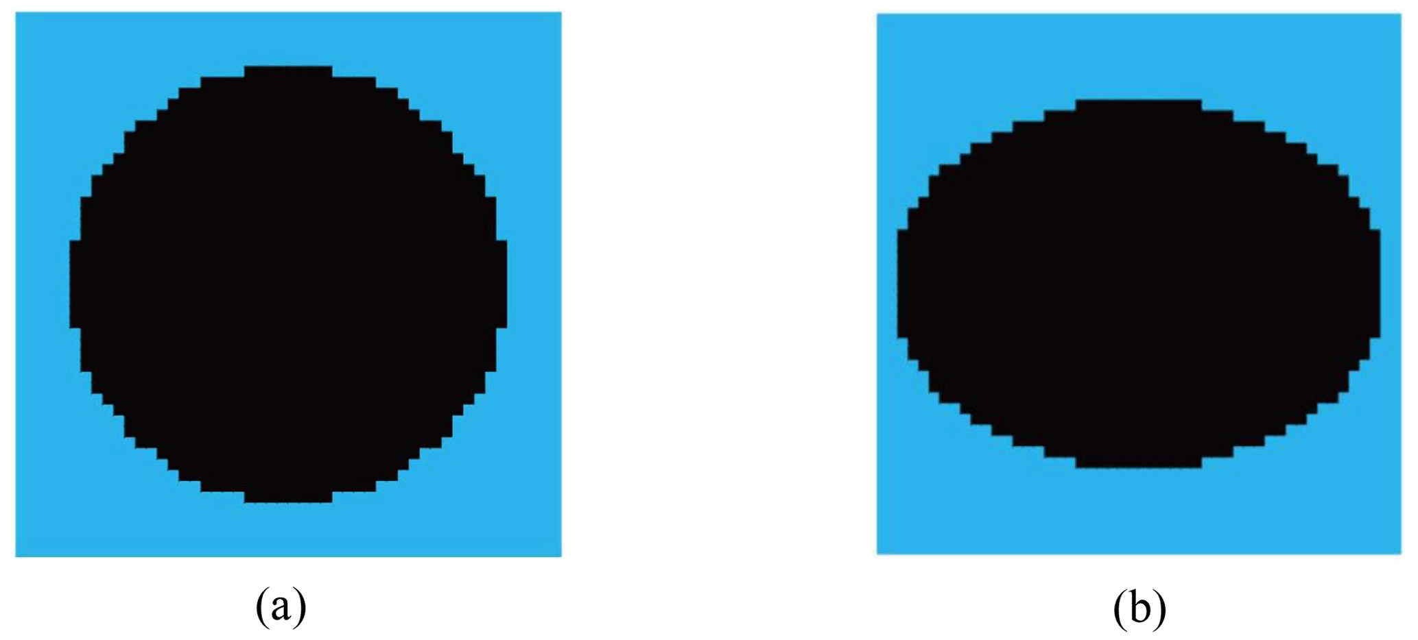
Figure 12Comparison of configurations for isotropic and orthotropic thermal conductivity: (a) isotropy with , ; (b) orthotropy with , .
As mentioned in Fig. 10, the design dependence of convection boundaries has an influence on the final optimal configuration. If the design-dependent convection boundary becomes a fixed boundary, with the G matrixes of the internal elements of the structure set as a constant zero matrix during iterations (see Fig. 13a), the iterative curves (see Fig. 13b) and topological configurations (see Fig. 13c) resemble those (see Fig. 13e, f) under fixed temperature constraints (see Fig. 13d), which illustrates that the essence of the convection boundary under the S23 condition is to dissipate heat from the structure. Moreover, compared with the optimal process curves, the convergence of the proposed method (36 iterations) is comparable to that of the traditional BESO method (36 iterations).
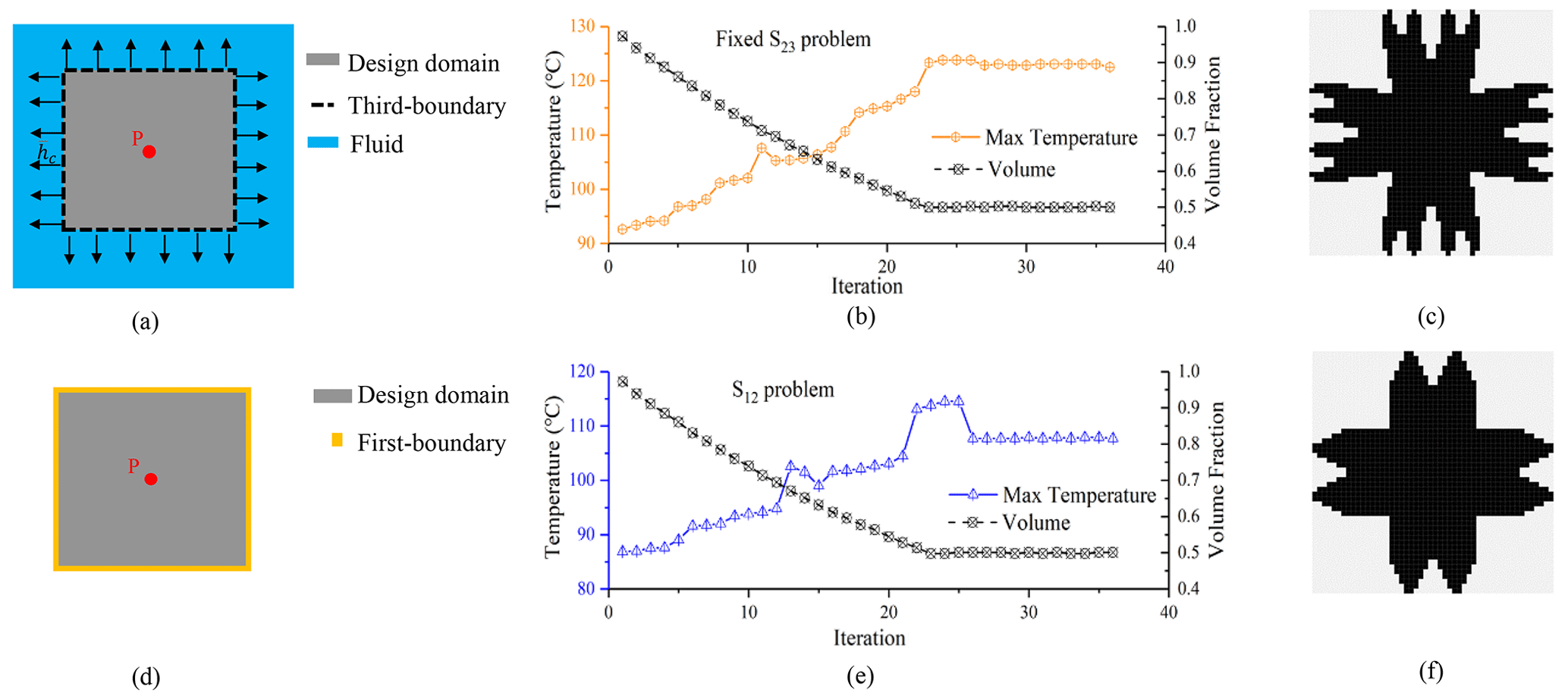
Figure 13Comparison of the results for the fixed S23 and S12 problems: (a) initial conditions for the fixed S23 problem; (b) optimal process for the fixed S12 problem; (c) configuration for the fixed S23 problem; (d) initial conditions for the S12 problem; (e) optimal process for the S12 problem; (f) configuration for the S12 problem.
5.3 The S123 problem
In this subsection, the optimization of the thermal structure under a combination of conditions including the convection boundary, temperature constraint and heat flux are discussed, i.e., the S123 problem. The design domain is a rectangular 4 m ×2 m ×1 m parallelepiped, and the number of the corresponding elements is . The geometric center of the design domain has an equivalent temperature load P. The left plane of the design domain has the convection boundary, and the four corners of the right plane have temperature constraints; the remainder boundaries are adiabatic boundaries. In order to illustrate two cases, namely that the convection boundary (1) acts as a cooling boundary to dissipate heat or (2) provides heat to the structure, the ambient temperature T∞ is set to 0 and 200 ∘C, respectively. The initial conditions and topology results are shown in Fig. 14a.
In Fig. 14, when T∞=0, the topology process (as shown in Fig. 14b) resembles that under S23 conditions, and the proposed method can decrease the temperature of the structure by lessening the distance between the design-dependent convection boundaries and the heat source (Fig. 14c). When T∞=200, the topological process resembles that under S13 conditions, as shown in Fig. 14d, and the proposed method can decrease the rise in structural temperature through design-dependent convection boundaries in the remaining original convection areas (Fig. 14e). Therefore, it can be concluded that the topological variations in convection boundaries are related to the relative temperature of the convection to structure for the S123 problem.

Figure 14Initial conditions and optimization results for the S123 problem under different ambient temperatures: (a) initial conditions; (b) optimal process under T∞=0; (c) optimal configuration under T∞=0; (d) optimal process under T∞=200; (e) optimal process under T∞=200.
The present study emphasizes a topology optimization method under design-dependent convection conditions. The main conclusions are as follows:
-
A topology optimization method for a thermal structure with design-dependent convection boundaries is proposed by introducing auxiliary elements to identify the design-dependent convection boundary, employing label matrixes to assign convection-concerned matrixes and utilizing a more appropriate optimal objective to address the design-dependent loads and heat transfer properties induced by convection changes.
-
The effectiveness of the proposed topological method is illustrated using cases with complex thermal boundary conditions (the S12, S13 and S123 problems). For all of the simulated cases, the proposed method can give reasonable topological configurations, and the corresponding convergence is comparable to that of the traditional BESO method.
-
In the S13 problem, as the design-dependent convection boundaries provide heat to the structure, the proposed method can reduce the temperature increase without expanding the convective boundary areas (e.g., the temperature dropped sharply from 83.19 to 70.31 ∘C from iteration 6 to iteration 7, as shown in Figs. 5a and 6). In the S23 problem, the design-dependent convection boundaries function to dissipate heat from the structure. The proposed method can decrease the structural temperature by lessening the distance between convection boundaries and the heat source (the second-type boundary). In the S123 problem, as a comprehensive combination of three types of boundaries, the convection boundaries' performance with respect to providing loads or dissipating heat depends on the relative temperature of the convection to the structure.
-
In the S13 problem, with constant convection boundaries, although taking the thermal compliance as the optimization objective is valid, a lower maximum temperature of the structure can be reached when taking the maximum temperature as the objective (77.44 ∘C vs. 80.12 ∘C with the former objective). In the S23 problem, with varying convection boundaries, from the iterative process and calculation results, it is obvious that the optimization objective of the maximum temperature proposed in this paper can still lead to a good topological optimal configuration with both a lower temperature of 88.42 ∘C and a thermal compliance of 8.84 kJ, whereas the thermal compliance objective is invalid because of the nonequivalence of the thermal compliance minimum and the heat transfer capability maximum under varying convective boundary conditions, which can result in an obviously higher temperature of 98.35 ∘C and a thermal compliance of 9.84 kJ, as seen from Fig. 10.
Without convection, the equivalent temperature load is independent of topological variables, and Eq. (21) can be simplified as follows:
When considering convective heat transfer, PT is no longer a fixed value, which is related to the change in the topological variable x. In this circumstance, Eq. (21) can be transformed into
The corresponding discrete forms of Eqs. (A1) and (A2) are as follows:
Under the SIMP penalization model, from Eq. (7), the heat transfer matrix without convection of elements can be expressed as follows:
The sensitivity αe without convection is then obtained, i.e.,
Combined with the SIMP model, Eqs. (5) and (13) are rewritten as follows:
Taking the derivatives of Eqs. (A7) and (A8), we have
The sensitivity αi considering convection is then derived as follows:
The original code and data used and/or analyzed in the current study are available upon reasonable request from the corresponding author.
YG: conceptualization, methodology and writing – original draft preparation; DW: project administration; TG: data curation; XL: investigation; XY: validation; GX: resources; LC: supervision, conceptualization and writing – review and editing.
The contact author has declared that none of the authors has any competing interests.
Publisher's note: Copernicus Publications remains neutral with regard to jurisdictional claims in published maps and institutional affiliations.
The authors gratefully acknowledge financial support from the Independent Innovation Foundation of the Aero Engine Corporation of China (AECC).
This research has been supported by the Independent Innovation Foundation of the AECC (grant no. ZZCX-2018-017).
This paper was edited by Haiyang Li and reviewed by Guangrong Chen and three anonymous referees.
Ahn, S.-H. and Cho, S.: Level Set-Based Topological Shape Optimization of Heat Conduction Problems Considering Design-Dependent Convection Boundary, Numer. Heat Tr. B-Fund., 58, 304–322, https://doi.org/10.1080/10407790.2010.522869, 2010.
Alexandersen, J.: Topology Optimization for Convection Problems, https://doi.org/10.13140/RG.2.2.24635.72485, 2011.
Bruns, T. E.: Topology optimization of convection-dominated, steady-state heat transfer problems, Int. J. Heat Mass Tran., 50, 2859–2873, https://doi.org/10.1016/j.ijheatmasstransfer.2007.01.039, 2007.
Chamkha, A. J., Rashad, A. M., Mansour, M. A., Armaghani, T., and Ghalambaz, M.: Effects of heat sink and source and entropy generation on MHD mixed convection of a Cu-water nanofluid in a lid-driven square porous enclosure with partial slip, Phys. Fluids, 29, 052001, https://doi.org/10.1063/1.4981911, 2017.
Coffin, P. and Maute, K.: Level set topology optimization of cooling and heating devices using a simplified convection model, Struct. Multidiscip. O., 53, 985–1003, https://doi.org/10.1007/s00158-015-1343-8, 2015.
Da, D., Xia, L., Li, G., and Huang, X.: Evolutionary topology optimization of continuum structures with smooth boundary representation, Struct. Multidiscip. O., 57, 2143–2159, https://doi.org/10.1007/s00158-017-1846-6, 2018.
Deaton, J. D. and Grandhi, R. V.: Stress-based design of thermal structures via topology optimization, Struct. Multidiscip. O., 53, 253–270, https://doi.org/10.1007/s00158-015-1331-z, 2015.
Deb, K. and Srivastava, S.: A genetic algorithm based augmented Lagrangian method for constrained optimization, Comput. Optim. Appl., 53, 869–902, https://doi.org/10.1007/s10589-012-9468-9, 2012.
Dede, E. M., Joshi, S. N., and Zhou, F.: Topology Optimization, Additive Layer Manufacturing, and Experimental Testing of an Air-Cooled Heat Sink, J. Mech. Design, 137, 111403, https://doi.org/10.1115/1.4030989, 2015.
Deshmukh, P. A. and Warkhedkar, R. M.: Thermal performance of elliptical pin fin heat sink under combined natural and forced convection, Exp. Therm. Fluid Sci., 50, 61–68, https://doi.org/10.1016/j.expthermflusci.2013.05.005, 2013.
Fuchs, M. and Moses, E.: Optimal structural topologies with transmissible loads, Struct. Multidiscip. O., 19, 263–273, https://doi.org/10.1007/s001580050123, 2000.
Gan, N. and Wang, Q.: Topology optimization of multiphase materials with dynamic and static characteristics by BESO method, Adv. Eng. Softw., 151, 102928, https://doi.org/10.1016/j.advengsoft.2020.102928, 2021.
Ho Yoon, G. and Young Kim, Y.: The element connectivity parameterization formulation for the topology design optimization of multiphysics systems, Int. J. Numer. Meth. Eng., 64, 1649–1677, https://doi.org/10.1002/nme.1422, 2005.
Hu, X. J., Jain, A., and Goodson, K. E.: Investigation of the natural convection boundary condition in microfabricated structures, Int. J. Therm. Sci., 47, 820–824, https://doi.org/10.1016/j.ijthermalsci.2007.07.011, 2008.
Huang, X. and Xie, Y. M.: Bi-directional evolutionary topology optimization of continuum structures with one or multiple materials, Comput. Mech., 43, 393–401, https://doi.org/10.1007/s00466-008-0312-0, 2008.
Huang, X. and Xie, Y. M.: Evolutionary topology optimization of continuum structures with an additional displacement constraint, Struct. Multidiscip. O., 40, 409–416, https://doi.org/10.1007/s00158-009-0382-4, 2009.
Huang, X. and Xie, Y.-M.: A further review of ESO type methods for topology optimization, Struct. Multidiscip. O., 41, 671–683, https://doi.org/10.1007/s00158-010-0487-9, 2010.
Iga, A., Nishiwaki, S., Izui, K., and Yoshimura, M.: Topology optimization for thermal conductors considering design-dependent effects, including heat conduction and convection, Int. J. Heat Mass Tran., 52, 2721–2732, https://doi.org/10.1016/j.ijheatmasstransfer.2008.12.013, 2009.
Li, H., Kondoh, T., Jolivet, P., Furuta, K., Yamada, T., Zhu, B., Zhang, H., Izui, K., and Nishiwaki, S.: Optimum design and thermal modeling for 2D and 3D natural convection problems incorporating level set-based topology optimization with body-fitted mesh, Int. J. Numer. Meth. Eng., 123, 1954–1990, https://doi.org/10.1002/nme.6923, 2022.
Palani, G. and Ganesan, P.: Heat transfer effects on dusty gas flow past a semi-infinite inclined plate, Forsch. Ingenieurwes., 71, 223–230, https://doi.org/10.1007/s10010-007-0061-9, 2007.
Pereira, R. L., Lopes, H. N., and Pavanello, R.: Topology optimization of acoustic systems with a multiconstrained BESO approach, Finite Elem. Anal. Des., 201, 103701, https://doi.org/10.1016/j.finel.2021.103701, 2022.
Picelli, R., Vicente, W., and Pavanello, R.: Bi-directional evolutionary structural optimization for design-dependent fluid pressure loading problems, Eng. Optimiz., 47, 1324–1342, https://doi.org/10.1080/0305215X.2014.963069, 2015.
Picelli, R., Vicente, W. M., and Pavanello, R.: Evolutionary topology optimization for structural compliance minimization considering design-dependent FSI loads, Finite Elem. Anal. Des., 135, 44–55, https://doi.org/10.1016/j.finel.2017.07.005, 2017.
Qiao, H., Wang, S., Zhao, T., and Tang, H.: Topology optimization for lightweight cellular material and structure simultaneously by combining SIMP with BESO, J. Mech. Sci. Technol., 33, 729–739, https://doi.org/10.1007/s12206-019-0127-2, 2019.
Radman, A.: Combination of BESO and harmony search for topology optimization of microstructures for materials, Appl. Math. Model., 90, 650–661, https://doi.org/10.1016/j.apm.2020.09.024, 2021.
Tavakoli, R. and Davami, P.: Optimal riser design in sand casting process by topology optimization with SIMP method I: Poisson approximation of nonlinear heat transfer equation, Struct. Multidiscip. O., 36, 193–202, https://doi.org/10.1007/s00158-007-0209-0, 2008.
Wah, B. W., Wang, T., Shang, Y., and Wu, Z.: Improving the performance of weighted Lagrange-multiplier methods for nonlinear constrained optimization, Inform. Sciences, 124, 241–272, https://doi.org/10.1016/S0020-0255(99)00081-X, 2000.
Wang, C. and Qian, X.: A density gradient approach to topology optimization under design-dependent boundary loading, J. Comput. Phys., 411, 109398, https://doi.org/10.1016/j.jcp.2020.109398, 2020.
Xia, Q., Shi, T., and Xia, L.: Topology optimization for heat conduction by combining level set method and BESO method, Int. J. Heat Mass Tran., 127, 200–209, https://doi.org/10.1016/j.ijheatmasstransfer.2018.08.036, 2018.
Xu, B., Han, Y., Zhao, L., and Xie, Y. M.: Topological optimization of continuum structures for additive manufacturing considering thin feature and support structure constraints, Eng. Optimiz., 53, 2122–2143, https://doi.org/10.1080/0305215x.2020.1849170, 2020.
Yan, X. Y., Liang, Y., and Cheng, G. D.: Discrete variable topology optimization for simplified convective heat transfer via sequential approximate integer programming with trust-region, Int. J. Numer. Meth. Eng., 122, 5844–5872, https://doi.org/10.1002/nme.6775, 2021.
Yang, X., Mühlenhoff, S., Nikrityuk, P. A., and Eckert, K.: The initial transient of natural convection during copper electrolysis in the presence of an opposing Lorentz force: Current dependence, Eur. Phys. J.-Spec. Top., 220, 303–312, https://doi.org/10.1140/epjst/e2013-01815-2, 2013.
Yang, X. Y., Xie, Y. M., and Steven, G. P.: Evolutionary methods for topology optimisation of continuous structures with design dependent loads, Comput. Struct., 83, 956–963, https://doi.org/10.1016/j.compstruc.2004.10.011, 2005.
Yin, L. and Ananthasuresh, G. K.: A novel topology design scheme for the multi-physics problems of electro-thermally actuated compliant micromechanisms, Sensor. Actuat. A-Phys., 97–98, 599–609, https://doi.org/10.1016/S0924-4247(01)00853-6, 2001.
Zhai, L., Fu, S., Lv, H., Zhang, C., and Wang, F.: Weighted Schatten p-norm minimization for 3D magnetic resonance images denoising, Brain Res. Bull., 142, 270–280, https://doi.org/10.1016/j.brainresbull.2018.08.006, 2018.
Zhou, K. and Li, X.: Topology optimization for minimum compliance under multiple loads based on continuous distribution of members, Struct. Multidiscip. O., 37, 49–56, https://doi.org/10.1007/s00158-007-0214-3, 2008.
Zhou, M., Alexandersen, J., Sigmund, O., and Pedersen, C. B. W.: Industrial application of topology optimization for combined conductive and convective heat transfer problems, Struct. Multidiscip. O., 54, 1045–1060, https://doi.org/10.1007/s00158-016-1433-2, 2016.
Zhu, J.-H., Zhang, W.-H., and Xia, L.: Topology Optimization in Aircraft and Aerospace Structures Design, Arch. Comput. Method. E., 23, 595–622, https://doi.org/10.1007/s11831-015-9151-2, 2015.
- Abstract
- Introduction
- Problem statement
- Convection boundary identification and its assignment
- Implementation of topology optimization
- Case analysis and discussion
- Conclusion
- Appendix A: The detailed derivation process of the sensitivity considering design-dependent convection
- Code and data availability
- Author contributions
- Competing interests
- Disclaimer
- Acknowledgements
- Financial support
- Review statement
- References