the Creative Commons Attribution 4.0 License.
the Creative Commons Attribution 4.0 License.
 | 21 Apr 2023
Kinematic and dynamic characteristics' analysis of a scissor multi-rod ring deployable mechanism
Bo Han
Yuxian Yao
Yuanzhi Zhou
Yundou Xu
Jiantao Yao
Yongsheng Zhao
In this paper, the authors developed a double-layer ring truss deployable antenna mechanism (RTDAM) based on a scissor unit, which can be used as the deployment and support mechanism in large-aperture satellite antenna. Firstly, three configuration state diagrams of the scissor multi-rod RTDAM were displayed: folded, half-deployed, and deployed. The mechanism was decomposed into a closed-ring deployable mechanism unit and several non-closed-ring deployable mechanism units. The screw constraint topological diagram of the closed-ring deployable mechanism unit was drawn, and the number of degrees of freedom (DOFs) was calculated via the screw theory method. Then, the expressions for screw velocity and screw acceleration of each component in the resultant mechanism were analyzed, calculated, and solved. The screw velocity and screw acceleration of each component were obtained, and the six-dimensional velocity and acceleration of each component were obtained through screw conversion and recursion. Finally, using the Newton–Euler equation and virtual work principle, the dynamic equation of the RTDAM with an integral scissor multi-rod ring truss mechanism was established, and the theoretical analysis was validated through numerical calculation and simulation results. The RTDAM of the scissor multi-rod ring truss proposed in this paper has a single DOF and can be well applied to the large-aperture satellite antenna.
- Article
(12488 KB) - Full-text XML
- BibTeX
- EndNote


In recent years, due to the rapid development of aerospace science and technology, the demand for large/super-large deployable mechanisms with deployment scales of tens or even hundreds of meters has become rather time-critical (Song et al., 2017; Huang et al., 2022; Yang et al., 2022; Dai et al., 2020; Zhang et al., 2022; Wu et al., 2019; Cao et al., 2018). This urgency has made space deployable mechanisms vital; a particularly important application direction of the space deployable mechanism is their use as the deployment and support mechanism of satellite antennae (Wang et al., 2014). Hence, it is of great significance to carry out a series of studies on the main line of innovative design in space deployable antenna mechanisms as it will improve the international space science research level (Nie et al., 2017; Chen et al., 2017; Xing and Zheng, 2014). The truss mechanism has been widely used in satellite antennae due to its high overall stiffness, easy control of shape, and surface accuracy (Okhotkin et al., 2017), for example, the ring truss deployable antenna mechanism (RTDAM) on the US NISAR satellite (Kobayashi et al., 2019; Focardi and Harrell, 2019; Focardi and Vacchione, 2019) and the AstroMesh RTDAM of NGST (Meguro et al., 2000). In addition, there are circular scissor deployable antennas from Russian companies (Cherniavsky et al., 2005; Medzmariashvili et al., 2009) and frame deployable antennas on Japanese satellite ETS–VIII (Meguro et al., 2009).
Many studies on developable mechanisms were carried out. Han et al. (2019, 2020) synthesized the ring truss antenna deployable mechanism using the constraint synthesis method. Ma et al. (2021) proposed a novel modular parabolic cylindrical antenna with geometric scalability. Wang and Kong (2018) have studied various ways to construct deployable polyhedral mechanisms. Liu and Hao (2022) designed two types of space deployable mechanisms using the bistable flexible mechanism. Next, Shi et al. (2018) proposed a double-layer ring truss deployable antenna. Yang et al. (2018) proposed and developed a triangular prism mast with tape-spring hyperelastic hinges. Kiani et al. (2022) designed a deployable Kirigami antenna mechanism for MIMO applications. Tian et al. (2022) proposed a new multi-folded rib modular deployable antenna mechanism. Huang et al. (2022) proposed a new type of cylindrical deployable mechanism that was based on rigid origami. Zhang et al. (2009) designed a deployable operating mechanism for spacecraft hatch. Wang et al. (2022) proposed a new three-limb deployable mechanism able to form a large complex surface to support the curved membrane. Some scholars have also studied planar deployable mechanisms and created many configurations (Meng et al., 2022; Zhuang and Ju, 2014; Vu et al., 2006).
The large-aperture spatial deployable mechanism is a dynamic system with spatial multi-closed-ring coupling and a flexible mechanism. Chen et al. (2005) and Chen and You (2008) calculated some of the classical linkage mechanisms' kinematic characteristics when constituting a space deployable mechanism. He et al. (2021) carried out a numerical analysis of space deployable mechanisms based on the shape memory polymer. Chen et al. (2021) observed in experiments that state jumps occur in space deployable mechanisms working in alternating temperature environments, finding a method to reduce their influence. Xu et al. (2018, 2019, 2020) analyzed the module topology to establish the numerical model of the deployable truss antenna configuration. Dai and Xiao (2020) optimized the design and analysis of deployable antenna truss mechanisms with constrained dynamic characteristics. Zhao et al. (2015) established the kinematic and dynamic Hessian matrix of the mechanism based on the screw theory. Wang et al. (2014, 2015) proposed a type of synthesis method for deployable truss mechanisms based on a two-step topology synthesis method.
Many traditional space mechanisms and deployable antenna mechanisms were analyzed in the above-presented literature review. Thus, in this paper, the authors proposed a double-layer multi-rod RTDAM based on a scissor unit. The overall mechanism configuration was analyzed, followed by the mechanism decomposition. The number of DOFs of the mechanism was calculated based on the screw theory, and the screw velocity equation and screw acceleration equation of each mechanism component were established through the screw constraint topological diagram. The six-dimensional velocity and accelerations of each component were analyzed and solved recursively. Based on the Newton–Euler equation and virtual work principle, the dynamic equation of the whole mechanism was established, and numerical calculation and simulation verification were carried out. This paper aims to explore the kinematic and dynamic characteristics of the scissor multi-rod RTDAM and to lay the foundations for further research.
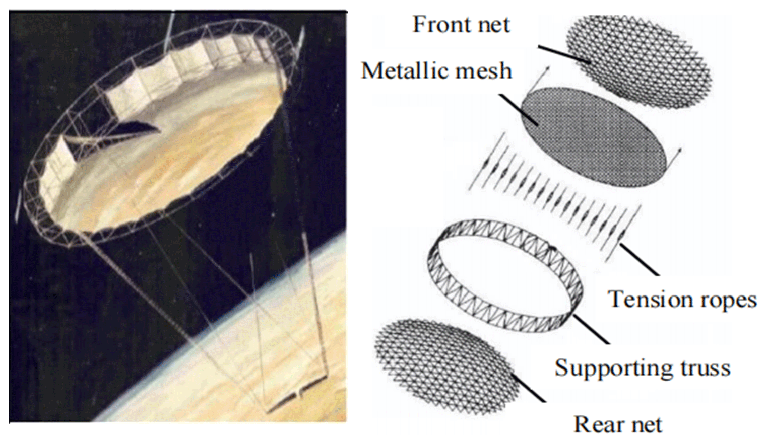
A truss space-deployable antenna generally comprises the ring truss, front and rear nets, metallic mesh, and multiple tension ropes. As shown in Fig. 1, the nodes are located at the front and rear ends of the peripheral ring truss. The front and rear nets are connected to the front and rear nodes, respectively. Further, metallic mesh is stretched into the shape of reflective paraboloids via multiple tension ropes installed between front and rear nets. The metallic mesh is attached to the nets and located in the intermediate of the front and rear nets. The scissor multi-rod RTDAM in this study acts as a ring of the whole antenna.
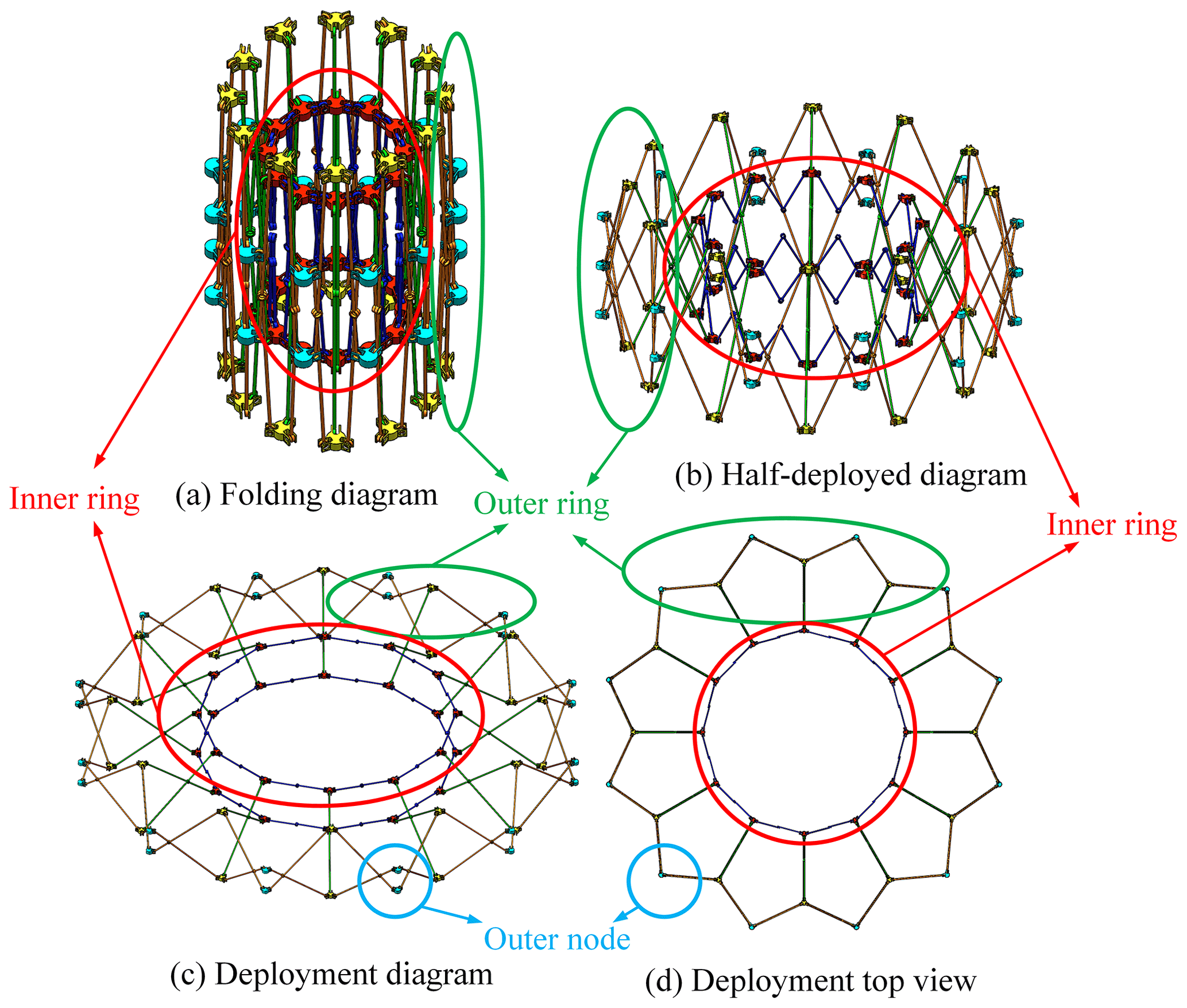
A scissor-type multi-rod RTDAM was shown in Fig. 2; it has a sunflower shape, as shown in Fig. 2d. The mechanism has high structural symmetry. By changing the number of scissor units in the whole mechanism and the length of their members, the RTDAM can be formed with different scales.
The mechanism shown in Fig. 2 is comprised of N scissor units, where N is a positive integer greater than or equal to 3. The scissor unit consists of 10 nodes, two pairs of 3R connecting rods (R stands for revolute joint), and four pairs of scissor rods. Multiple scissor units are arranged in an array, with adjacent units being connected by sharing two pairs of outer nodes and two intermediate nodes.
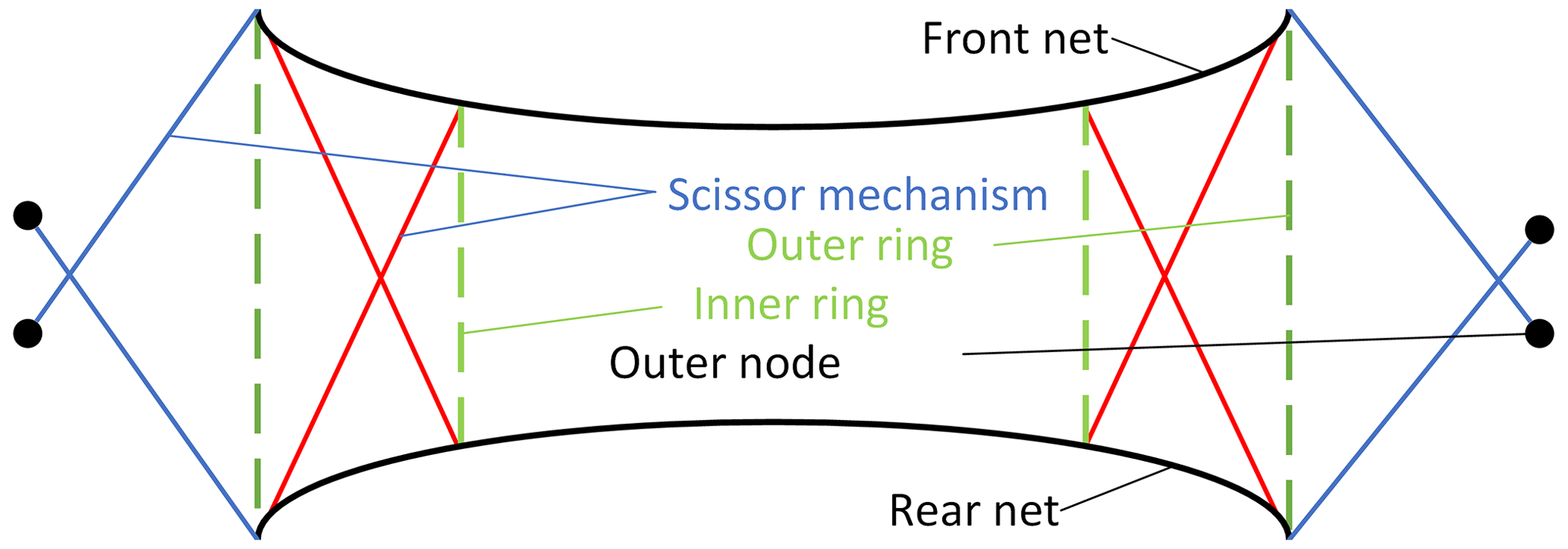
The RTDAM is the antenna deployment and support mechanism. The front and rear nets are connected to the ring truss mechanism, while the reflected net is connected to the front net by tension and stretched into a parabolic shape according to the tension. The double-layer RTDAM shown in this paper has no harsh geometric conditions due to the 3R mechanism which is included in the inner ring. The mechanism length can be designed flexibly and the outer ring truss can connect the network. The blue scissor rod (Fig. 3) is mounted between the outer ring and the outer node and can improve the structural stiffness of the ring truss when deployed. Moreover, its outer node has a limited influence on the overall size of the RTDAM when folded.
This antenna mechanism has three states – deployed, half-deployed, and folded. The deployed state refers to the mechanism state when it works in outer space and is the primary working state. The half-deployed state is the primary area of this study; it refers to the mechanism movement and mainly reflects its performance. Finally, the folded state reduces the occupied space of the mechanism itself, reducing transportation costs. The kinematic joints in the mechanism are all revolute joints, and the outer ring truss and the inner ring truss are connected through the intermediate scissor rod.
3.1 DOF analysis of the closed-ring deployable mechanism unit
A spatial Cartesian coordinate system was established for the closed-ring deployable mechanism unit, as shown in Figs. 4 and 5. The coordinate system origin O is located at the center of the bottom node G. The X axis points from node G to the projection of the intermediate node (node H,I) on the bottom. The Z axis points up towards the outer node C, while the Y axis is determined using the right-hand rule.

In Fig. 4, each node is marked with capital letters, while the rod number is represented by the marks of the node it joins. For example, the number of scissor rods between nodes A and G is AG, and the numbers of two connecting rods between nodes D and E are DE1 and DE2, respectively. Other components follow the same naming convention.
The length of the intermediate scissor rods (rods AG, CD, BJ, and EF) connected with the inner node (nodes A, B, D, and E) is p, while the length of the section connected to the outer nodes (nodes C, F, G, and J) is q. Further, r marks the length of an outer scissor rod section connected to the intermediate node (nodes H and J). The length of the inner scissor rods (AB1, AB2, DE1, and DE2) connected to the inner node is h. The angle between the intermediate scissor rods is designated as θ1, while θ2 is the angle between the inner connecting rods. The distance between each revolute joint axis on the inner node and the center is l. Moreover, the distance between the axis of each revolute joint located on the outer node and the center is m, and lastly, the distance between the axis of each revolute joint located on the intermediate node and the center is n.
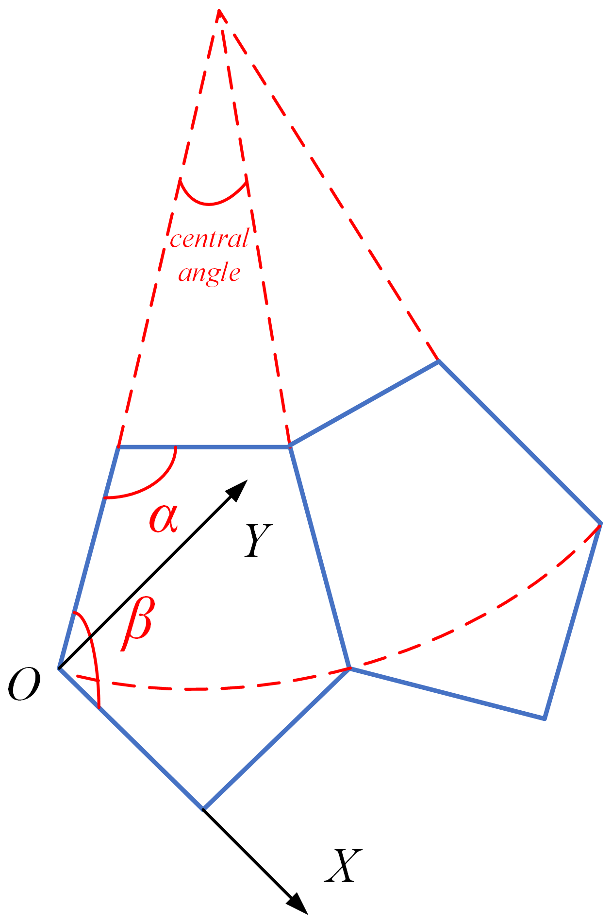
In Fig. 5, included angles of forks on the inner and outer nodes are α and β, respectively. Furthermore, the following relationship between the parameters in Figs. 4 and 5 holds:
In Eq. (1), the symbolic expression is as follows:
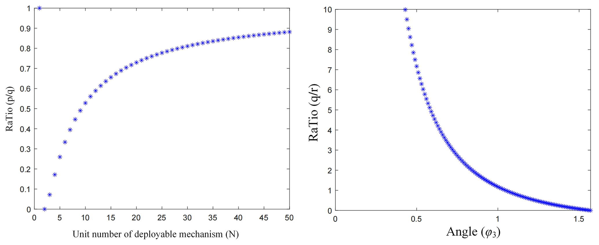
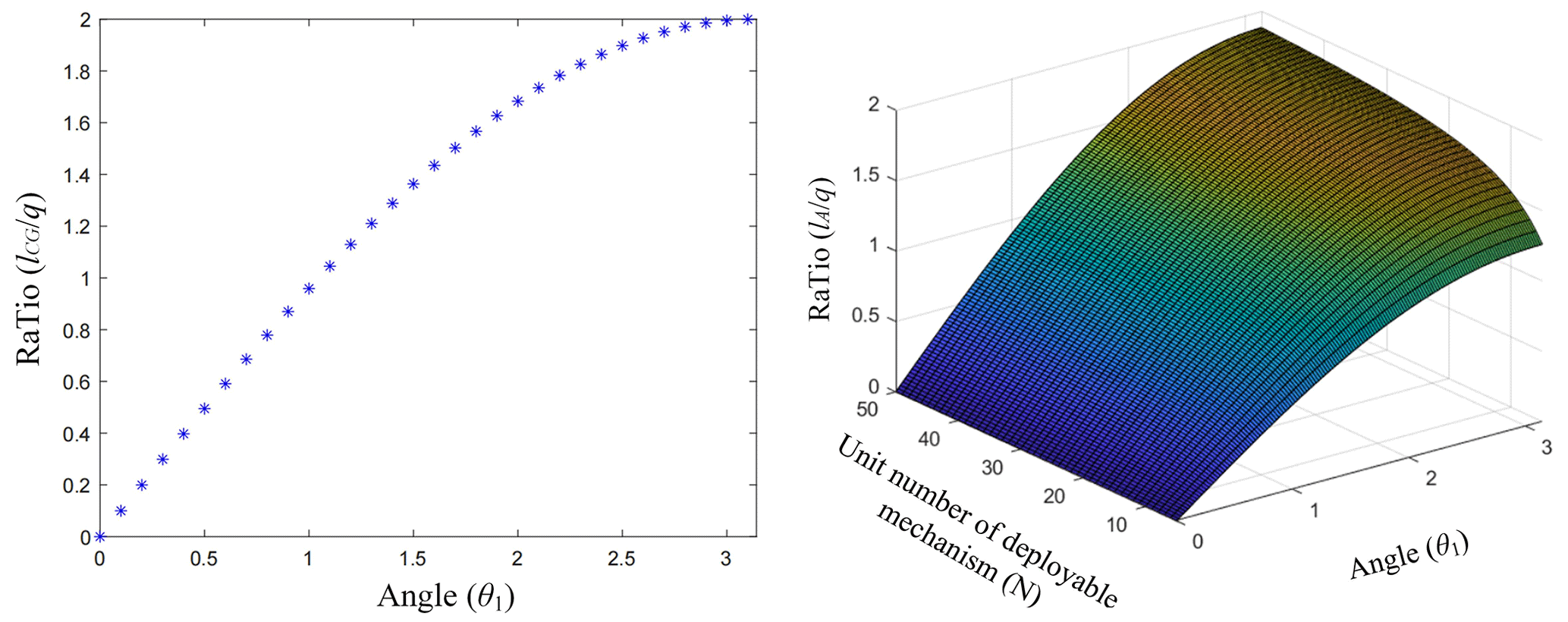
The proportional relationship formula and the proportional relationship diagram between components can be obtained from Figs. 4 and 5:

In Eq. (5), the symbol is related as follows:
In Eqs. (7) and (8), the variable lCG represents the distance between the node C and G, while lA is the projection distance between the node A and the plane O–XY.
Furthermore, the spatial position coordinates of the revolute joint 25 connecting the rod CI and the rod GH, as well as the axial direction of the revolute shaft of the revolute joint 25, can be obtained from Fig. 4, as follows:
In Fig. 9, members are represented by circles, revolute joints are represented by lines, and movements at different joints are represented by digital kinematic screws. For example, the screw constraint topological diagram of the closed-ring deployable mechanism unit can be obtained using $5 to represent the movement of the revolute joint connecting rods AG and CD. The relative revolution velocity between the two components can be divided into two parts: a vector representing the direction of the velocity and a scalar representing the value of the velocity. The direction of the arrow in Fig. 9 corresponds to the direction of the revolute joint, and when the direction of the arrow changes, the calculated velocity scalar will also change. Therefore, the arrow direction will not affect the final calculation.
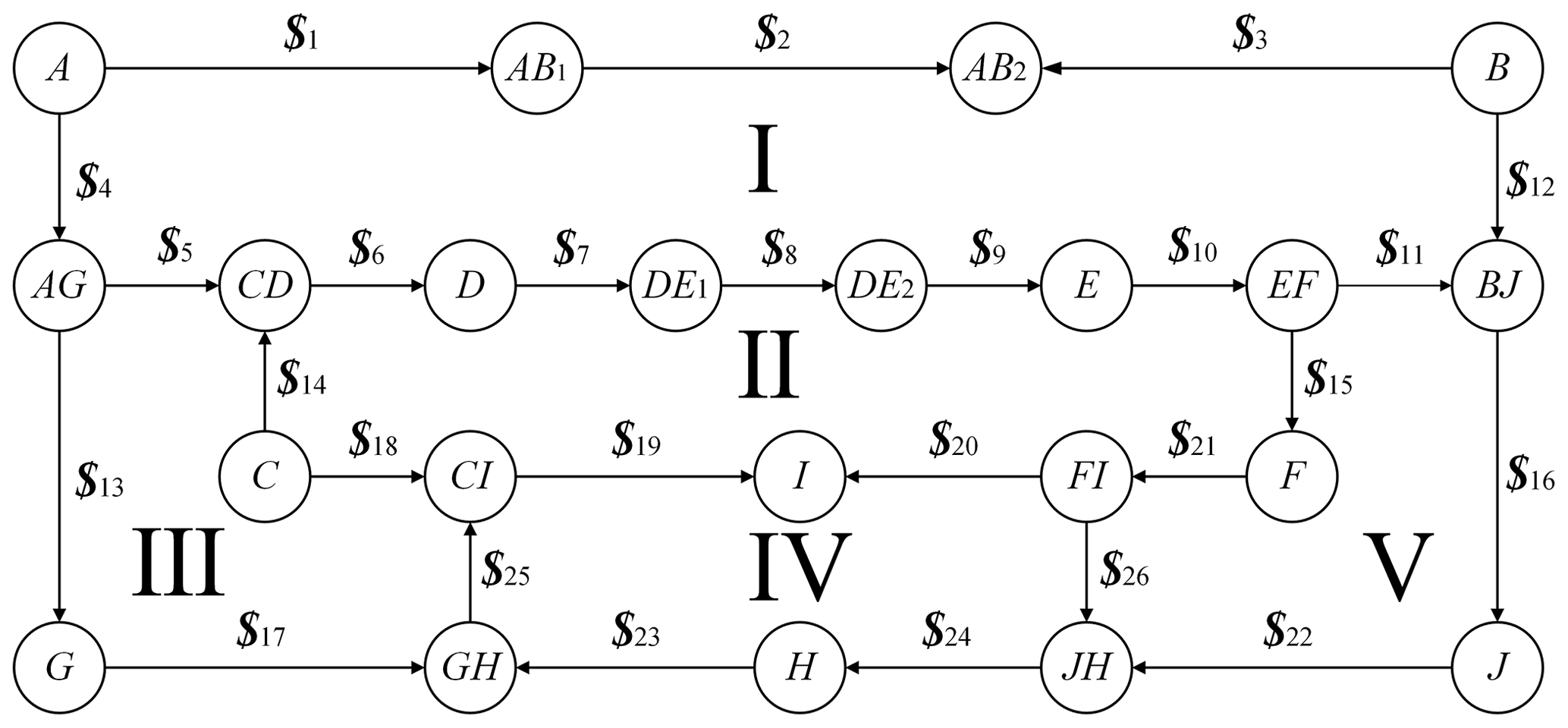
Figure 9Topology diagram of the screw constraint of the closed-ring deployable mechanism unit.
Using Fig. 9, the expression of the revolute joint unit 25 movement screw can be obtained as follows:
On this basis, and combined with the functional relationship between the rod and the node shown in Fig. 4, expressions can also be obtained for other motion screws (shown in Fig. 9).The corresponding screw constraint equations are established based on the five closed rings (i–v, shown in Fig. 9), and the corresponding screw constraint equations are written as follows:
In Eq. (12), the symbolic expressions are as follows:
Regarding Eqs. (12) and (13), symbol meanings are as follows: ωi is the angular velocity of the revolute joint i in the mechanism unit, and 0 is a six-dimensional zero vector.
By combining Eqs. (12) and (13) to record the matrix containing ωi as the unknown matrix W, the expression of the unknown matrix W is written as follows:
The matrix containing $i is written as the coefficient matrix Q, and the expression of the coefficient matrix Q is as follows:
Finally, Eq. (15) symbols are expressed as
In Eq. (16), symbols 0 and $i are six-dimensional zero vectors.
Equations (12) and (13) can be written in the form of a matrix according to the unknown matrix W and the coefficient matrix Q:
The screw constraint matrix Q in Eq. (17) is a 30 × 26 matrix. The number of DOFs of the closed-ring deployable mechanism unit corresponds to the dimension of the screw constraint matrix zero space, which can be calculated using MATLAB:
In Eq. (18), rank(•) represents the matrix rank.
The number of columns of the screw constraint matrix Q is 26, and the dimension of its null space is the number of columns minus its rank. Therefore, the obtained number of DOFs of the closed-ring deployable mechanism element was 1.
3.2 DOF analysis of the scissor multi-rod RTDAM
The mechanism of the double-layer RTDAM can be decomposed into a closed-ring deployable mechanism unit and multiple non-closed-ring deployable units, as shown in Fig. 4.
As shown in Fig. 10, the non-closed-ring deployable mechanism units only contains one type, as shown in Fig. 11.
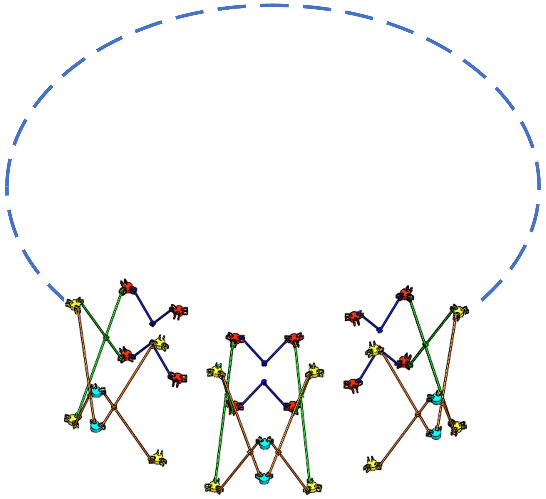
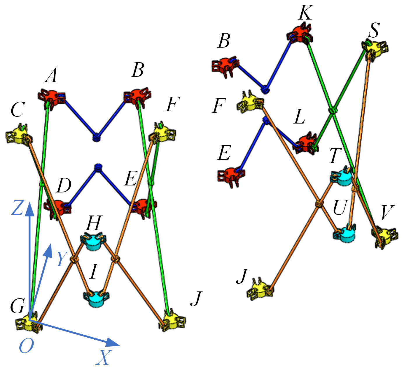
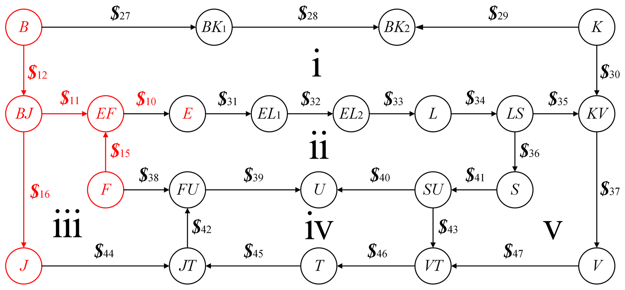
Figure 12Topology diagram of the screw constraint of the non-closed-ring deployable mechanism unit.
The closed-ring deployable mechanism unit and coordinate systems are those shown in Fig. 11. The node of the right mechanism unit is numbered with capital letters; the numbering convention and arrow direction for rods and revolute joints are the same as outlined in the previous section. The screw constraint topological diagram of the non-closed-ring deployable mechanism unit in Fig. 11 can be obtained and is shown in Fig. 12.
The screw constraint equations are established for the five closed rings (i–v) shown in Fig. 12, with the screw constraint equations obtained as follows:
In Eq. (19), the symbolic expressions are
In Eq. (20), symbol meanings are as follows: ωi is the angular velocity of the revolute joint i in the mechanism unit, and 0 is a six-dimensional zero vector.
In Fig. 11, the nodes B, E, F, and J, the intermediate scissor mechanism (rods BJ and EF), and the five revolute joints connected to them are shared by the two mechanism units. When Eqs. (12), (13), (19), and (20) are combined, revolute joints shared by the mechanism units are calculated repeatedly. Hence, when calculating the DOFs of the unit combination mechanism, the repeatedly calculated kinematic screw should be removed. In other words, $10, $11, $12, $15, and $16 should only be calculated once. Here, the repeatedly calculated screw motion in the non-closed-ring deployable mechanism unit was removed (the red part in Fig. 12).
The matrix containing ωi in Eqs. (19) and (20) is regarded as an unknown matrix W′ and expressed as
The matrix containing $i is written as the coefficient matrix Q′ and expressed as
with symbols expressed as follows:
In Eq. (23), 0 and $i are six-dimensional zero vectors.
Equations (19) and (20) are written as matrices according to the unknown matrix W′ and the coefficient matrix Q′, as follows:
Further, in Eq. (18), the screw constraint matrix Q′ is a 30 × 21 matrix and can be calculated via MATLAB:
After combining Eqs. (17) and (24), the screw constraint equations of the unit combination mechanism can be obtained:
In Eq. (26), the coefficient matrix U is
The unknown matrix V is
It can be seen from Eq. (27) that the matrix U rank mainly depends on matrices Q and Q′. The rank of the coefficient matrix U can be easily obtained through Eqs. (18) and (25) using MATLAB:
It can be concluded that the number of DOFs of the combined mechanism is equal to the number of the coefficient matrix U columns minus its rank; the obtained DOF value is 1. Therefore, the number of DOFs of the combined mechanism is equal to that of a single closed-ring deployable mechanism unit.
When the non-closed-ring deployable mechanism unit is continuously added based on the combined mechanism, as shown in the prior analysis, the overall mechanism number of DOFs remains the same as that of a single closed-ring deployable mechanism unit. Through the same analysis, when a single closed-ring deployable mechanism unit is joined with multiple non-closed-ring deployable mechanism units to form a scissor multi-rod RTDAM, its overall number of DOFs remains the same as that of a single closed-ring deployable mechanism unit. Hence, the whole scissor multi-rod RTDAM has only 1 DOF. Since the number of DOFs of the component movements in the mechanism is less than or equal to that of the whole mechanism, each moving component in the scissor multi-rod RTDAM has only 1 DOF.
4.1 Unit velocity analysis of the closed-ring deployable mechanism
Based on the analysis provided in Sect. 3.2, the unit combination mechanism is a single-DOF mechanism. Thus, given one of the inputs (ω17), the angular velocity of each component can be found using the screw constraint equations provided in Eqs. (12), (13), (19), and (20). Furthermore, based on the configuration relationship of the unit combination mechanism and the screw constraint topological diagram (shown in Figs. 9 and 12), the screw velocity of each component can be obtained through screw operation.
In the coordinate system with the node G as the coordinate origin (see Fig. 4) and the screw constraint topological diagram (Fig. 9), the screw velocity of each component in the closed ring III is calculated as
where 0 is a six-dimensional zero vector, and Vi represents the screw velocity of component i.
In the closed ring IV of the screw constraint topological diagram (Fig. 9), the screw velocities of the components CI and GH are obtained via Eq. (30). Screw velocities of other closed ring IV components can be calculated from the previously obtained screw velocities. Based on the screw velocity of component GH, the screw velocity of other components in closed ring IV is
Similarly, the screw velocity of each component in closed rings I, II, and V (Fig. 9) and closed rings i–v (Fig. 12) can also be solved in turn.
According to the physical meaning of the velocity screw, the angular velocity coordinate quantity and linear velocity quantity of each component are
where ω(•) represents the original part of the velocity screw (the first three terms), and ν(•) is the dual part of the velocity screw (the last three terms).
Therefore, the linear velocity of the center of mass of the component is
where ri is the vector from the coordinate origin to the centroid position of the component.
Through the above-presented analysis and calculation, the angular and linear velocity at the center of mass of the closed-ring deployable mechanism unit can be solved.
4.2 Velocity analysis of other closed-ring deployable mechanisms
Since closed-ring deployable mechanism units in the scissor multi-rod RTDAM have the same size, each unit moves to the center of the ring truss during the movement. Therefore, if the coordinate system is established at the same position of each closed-ring deployable mechanism unit, and the direction of the coordinate system remains the same, the member with the same position in each closed-ring deployable mechanism unit will have equal velocities in their coordinate systems.
As shown in Fig. 13, the velocity of each component of the expandable closed-ring deployable mechanism unit in Sect. 4.1 was obtained in the coordinate system O–XYZ of the unit shown on the left side of Fig. 13. The coordinate system O1–X1Y1Z1 was established for the coordinate origin at the node J of the closed-ring deployable mechanism unit adjacently on the right side. Then, the velocity of the node B in the coordinate system O–XYZ is the same as that of the node K in the coordinate system O1–X1Y1Z1, which can be expressed as
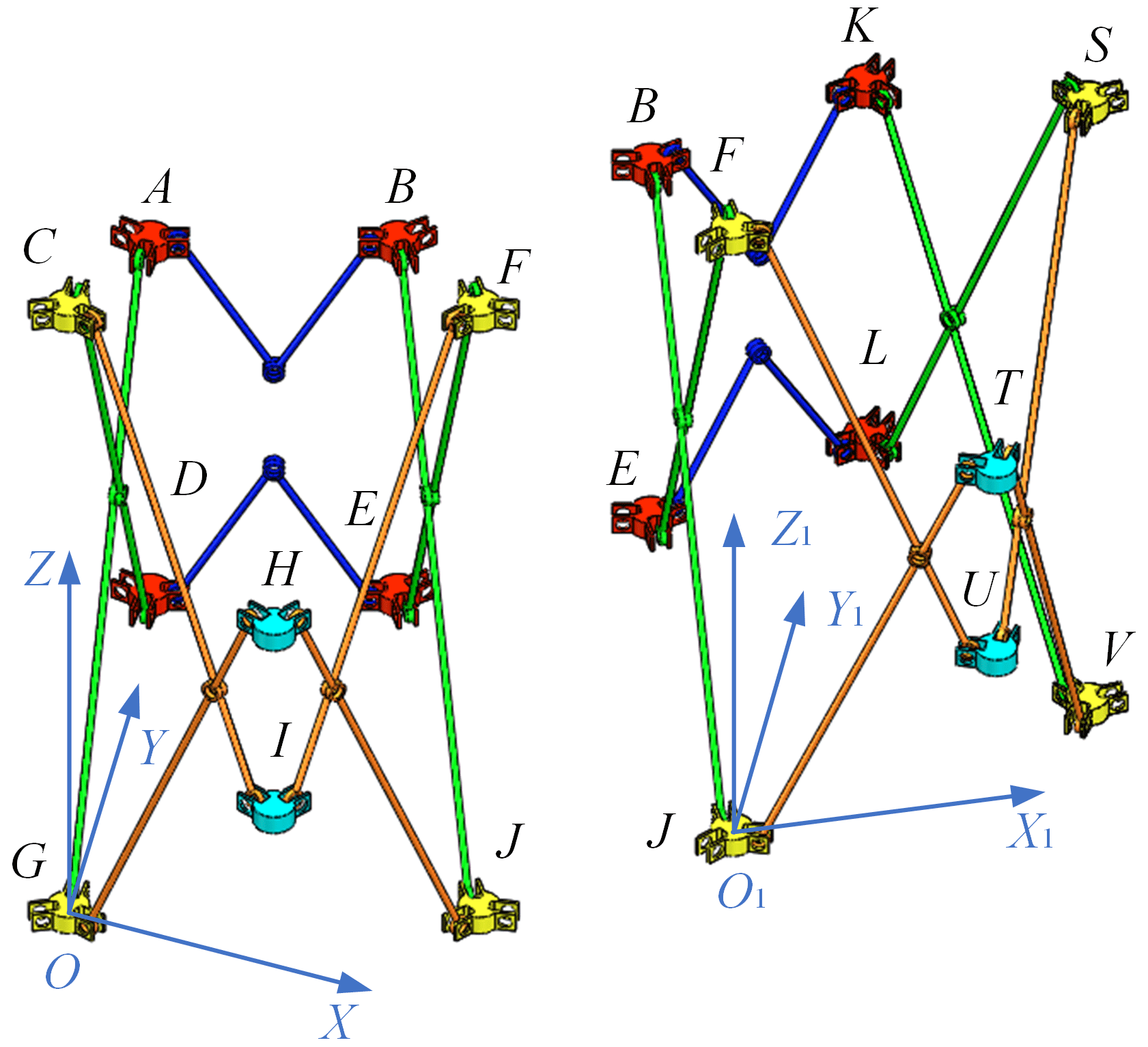
Other components in the closed-ring deployable mechanism unit shown on the right side of Fig. 13 have similar relationships. The same principle can be extended to the remaining scissor multi-rod ring trusses. Kinematic relationships among other closed-ring deployable mechanism units are also shown in Fig. 13 using two closed-ring deployable basic units. If the double-layer multi-rod RTDAM can be divided into N closed-ring deployable mechanism units, then N coordinate systems can be established (O–XYZ to ON−1–). The selected coordinate system O–XYZ is the global coordinate system, and the included angle between the X axes of coordinate systems established by δ in adjacent units is , as shown in Fig. 14.
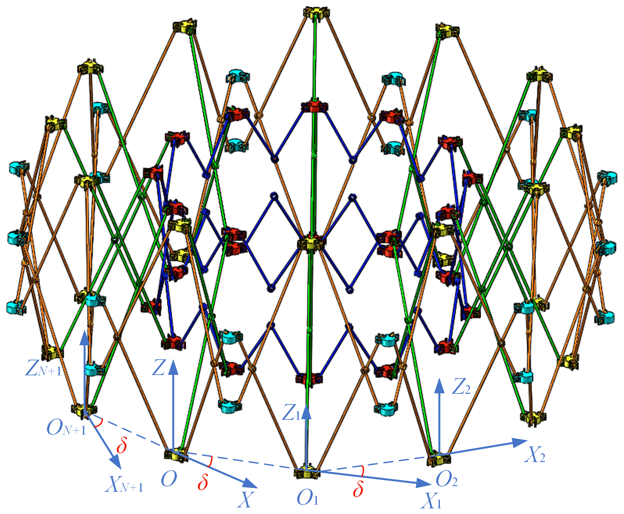
The selected coordinate system O–XYZ is the global coordinate system; the velocity of each component is expressed using the global coordinate system, as follows:
where k is the component number and j is the coordinate system number. The expression of the revolute transformation matrix can be written as
Through the analysis and calculation procedure shown above, the angular and linear velocities at the center of mass of each component in the mechanism can be solved and expressed in the global coordinate system.
After the angular velocity and centroid linear velocity of each component are obtained, the six-dimensional velocity vector of the component can be obtained by combining them. As the mechanism is a single-DOF mechanism, only one drive is required. Therefore, the Jacobian matrix of each component can be obtained by extracting the input velocity from the six-dimensional velocity vector of each component through symbolic operation:
where is the six-dimensional velocity vector of component i, Ji(ς) is the velocity Jacobian matrix of component i , and ς is the driving input of the whole mechanism (the driving angle function).
Screw acceleration can be expressed as
where Ai represents the screw acceleration of the ith mechanism component (the six-dimensional acceleration measurement of the coincidence point of the component reference coordinate system origin), εi is the angular acceleration measurement of the coincidence point of the origin of the component reference coordinate system, and a is the linear acceleration at the component centroid.
It is evident from Eq. (39) that, among the six-dimensional screw accelerations, the first three terms are the component angular velocity, and the last three terms represent the difference between its linear and centripetal acceleration.
The screw acceleration synthesis rule of a multi-rigid-body system is
where Lie[] is a Lie bracket operation, a six-dimensional vector.
If there are two screws,
where s1 is the original part of $1 (the first three terms), and is the dual part of $1 (the last three terms). The same is true for $2.
Next, the Lie bracket operation of the two screws is
By combining Fig. 9 and Eq. (40), the screw acceleration equations of each closed ring can be obtained. This includes the closed ring III shown in Fig. 9, for which we write
In Eq. (43), the symbolic expression is as follows:
Therefore, there are
Similarly, corresponding screw acceleration equations can be obtained for closed rings I, II, IV, and V shown in Fig. 9 and closed rings i–v in Fig. 12. When the input angular acceleration (e. g. ε17) is known, the screw acceleration of each component in the unit combination mechanism can be solved via Eq. (45) and other screw acceleration equations.
After finding the screw acceleration of each component, the corresponding angular accelerations can be obtained by extracting its original part:
In Eqs. (46) and (47), ε(•) represents the original part of the extracted screw acceleration (the first three terms), and a(•) is the dual part of the extracted screw acceleration (the last three terms).
The linear acceleration at the center of mass of the component is solved, yielding
Similar to the velocity analysis shown in Sect. 4, the acceleration of components with the same position in each unit combination mechanism is the same (in their coordinate system). The acceleration of components in each unit combination mechanism is expressed in the global coordinate system as
where k represents the component number, and j is the coordinate system number.
Based on the conducted analysis and calculation, the angular and linear accelerations of the center of mass of each component in the double-layer RTDAM can be solved and expressed in the global coordinate system.
6.1 Dynamic modeling
Using the Newton–Euler formula, we obtain
where F is the outer force of the component, m is the component mass, N is the moment of the component, and I is the component inertia tensor.
In the double-layer multi-rod RTDAM based on the scissor unit studied in this paper, the inertia force of each component can be obtained using
For each component in the unit combination mechanism, whose coordinate system coincides with the global coordinate system, the inertia moment of each component can be obtained through the following expression:
When calculating the inertia moment of components in the basic mechanism units of other coordinate systems, it is necessary to add a revolute transformation matrix. In that case, the expression of the inertia moment of each component in the global coordinate system is
Since the deployable antenna operates in space, which can be regarded as weightless, the inertia force and moment of each component are written in the form of a six-dimensional force vector without considering the influence of gravity:
According to the virtual work principle, the overall dynamic equation of the double-layer multi-rod RTDAM based on a scissor unit is as follows:
where T is the input matrix, and Ji is the component Jacobian matrix.
6.2 Numerical simulation verification of mechanism expandability and dynamics
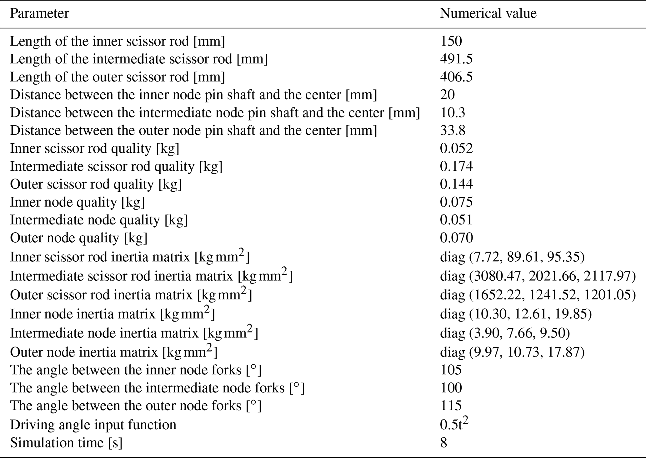
The simulation model of a double-layer multi-rod RTDAM based on a scissor unit is established. The dynamic simulation software ADAMS and MATLAB were used to carry out numerical calculations. The simulation model parameters are given in Table 1.
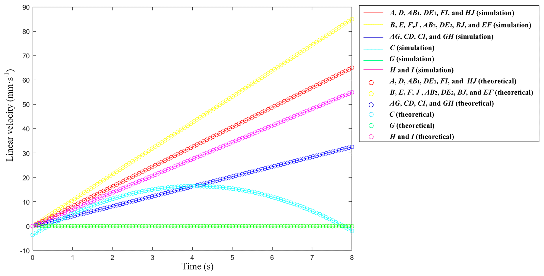

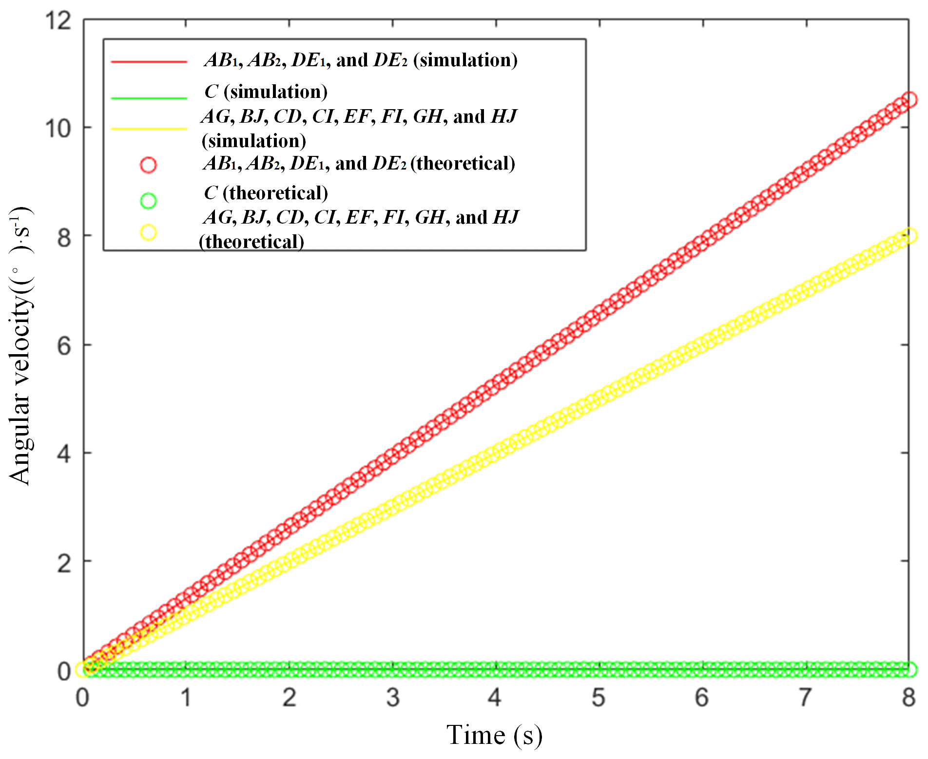
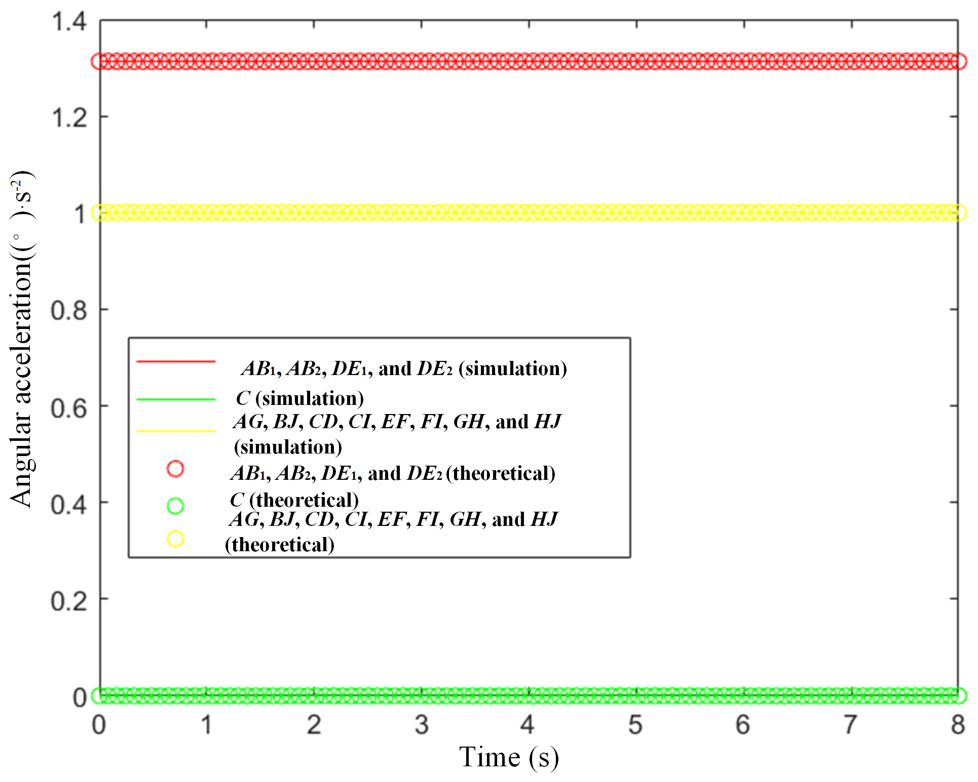
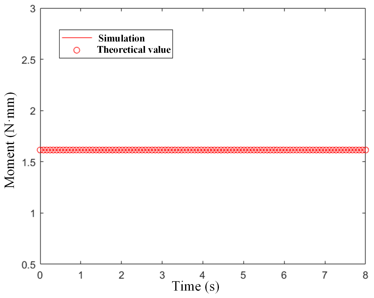
All scissor rods and all nodes in a deployable closed-ring mechanism unit in a local coordinate system consistent with the global coordinate system are selected as target components. The theoretical calculation results and simulation results are shown in Figs. 15–19.
As shown in each of the curves shown in Figs. 15 to 19, theoretical values were in agreement with simulation values, confirming the correctness of the analysis and calculation method of the kinematic model and dynamic model.
Figures 15 to 18 show that, in the truss mechanism in which the scissor mechanism occupies the main body, the velocity and acceleration of each component coincide. This coincidence is also in accordance with the scissor mechanism motion characteristics.
As shown in Figs. 17 and 18, the angular velocity and angular acceleration of all the nodes are zero during the movement of the whole scissor multi-rod RTDAM. That is, each node has only 1 movement DOF and no revolute DOFs, which is the result presented in this paper.
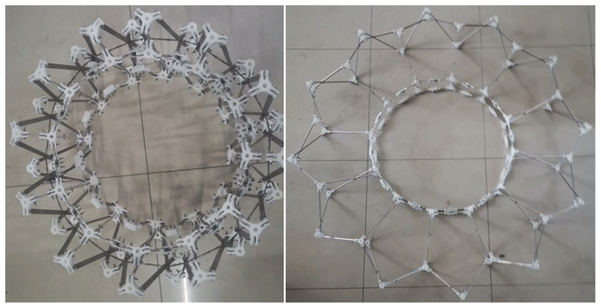
Based on the geometric parameters shown in Table 1, the mechanism prototype was made. Aiming to maintain geometric conditions, the prototype was made by 3D printing components and aluminum connecting rods. Prototype diagrams of the folded and deployed state of the prototype are shown in Fig. 20.
In this paper, a RTDAM suitable for satellites is designed. The distribution of connecting rods and nodes in the truss mechanism was discussed, and the unit was in the shape of a convex pentagon when viewed from the top. The unit DOFs and the whole DOFs of the mechanism were verified, and the velocity and acceleration of the rod and the node were calculated. Combined with theoretical analysis and software simulation, the rationality of the overall mechanism of the RTDAM and the correctness of the movement in the process of deployment-folding were verified. The main conclusions are detailed here.
A double-layer multi-rod RTDAM based on a scissor unit was proposed, and its DOFs were analyzed. It was calculated that the mechanism has only 1 DOF. The mechanism advantages include a simple mechanism and a low number of driving numbers; additionally, it can support and deploy large space antennas.
Both the theoretical and simulation models of the RTDAM with an integral scissor multi-rod ring truss mechanism were established. The kinematic model of the RTDAM was established by screw theory and Lie bracket operation, and the numerical calculation and simulation verification were carried out. The calculation and simulation results have verified the theoretical analysis results provided in this paper.
A prototype was made by 3D printing, and the prototype was established according to the ratio of 10:1. The diameter of the prototype was 0.4 m when it was completely folded and 1.4 m when it was deployed. And the prototype can complete the action of folding and deployment well in the process of testing.
Limited to the level of knowledge and experimental conditions, in this paper, the mechanism was theoretically calculated according to the knowledge of screw theory and mechanism, and the kinematic and dynamic models of the RTDAM were initially established. In the future, a flexible mathematical model of RTDAM will be established for more realistic dynamic calculation. In addition, the gravity unloading system will be established to simulate the weightless space environment more realistically, so as to complete the more detailed measurement of the prototype deployment process and get more accurate experimental data.
All the data used in this paper can be obtained by request from the corresponding author.
BH conceptualized the study and reviewed the paper. YY wrote the original draft and revised the paper. YZho analyzed the degrees of freedom. YX carried out kinematic analysis. JY carried out dynamic analysis. YZha carried out the simulation analysis.
The contact author has declared that none of the authors has any competing interests.
Publisher's note: Copernicus Publications remains neutral with regard to jurisdictional claims in published maps and institutional affiliations.
This work was supported by the National Natural Science Foundation of China (grant nos. 52105035 and 52075467), the Natural Science Foundation of Hebei Province of China (grant no. E2021203109), the State Key Laboratory of Robotics and Systems (HIT) (grant no. SKLRS-2021-KF-15), and the Industrial Robot Control and Reliability Technology Innovation Center of Hebei Province (grant no. JXKF2105).
This research has been supported by the National Natural Science Foundation of China (grant nos. 52105035 and 52075467), the Natural Science Foundation of Hebei Province of China (grant no. E2021203109), the State Key Laboratory of Robotics and Systems (HIT) (grant no. SKLRS-2021-KF-15), and the Industrial Robot Control and Reliability Technology Innovation Center of Hebei Province (grant no. JXKF2105).
This paper was edited by Daniel Condurache and reviewed by two anonymous referees.
Cao, W. A., Yang, D. H., and Ding, H. F.: Topological structural design of umbrella-shaped deployable mechanisms based on new spatial closed-loop linkage units, J. Mech. Design, 140, 062302, https://doi.org/10.1115/1.4039388, 2018.
Chen, C., Li, T., Tang, Y., and Wang, Z.: Analysis and control of state jump in space deployable structures under alternating temperature loads, Mech. Sci., 12, 59–67, https://doi.org/10.5194/ms-12-59-2021, 2021.
Chen, Y. and You Z.: On mobile assemblies of Bennett linkages, P. Roy. Soc. A-Math. Phy., 464, 1275–1293, https://doi.org/10.1098/rspa.2007.0188, 2008.
Chen, Y., You, Z., and Tarnai, T.: Threefold-symmetric Bricard linkages for deployable structure, Int. J. Solids Struct., 42, 2287–2301, https://doi.org/10.1016/j.ijsolstr.2004.09.014, 2005.
Chen, Y., Feng J., and Sun, Q. Z.: Lower-order symmetric mechanism modes and bifurcation behavior of deployable bar structures with cyclic symmetry, Int. J. Solids Struct., 139–140, 1–14, https://doi.org/10.1016/j.ijsolstr.2017.05.008, 2017.
Cherniavsky, A. G., Gulyayev, V. I., Gaidaichuk, V., and Fedoseev, A. I.: Large deployable space antennas based on usage of polygonal pantograph, J. Aerospace Eng., 18, 139–145, https://doi.org/10.1061/(ASCE)0893-1321(2005)18:3(139), 2005.
Dai, L. and Xiao, R.: Optimal design and analysis of deployable antenna truss structure based on dynamic characteristics restraints, Aerosp. Sci. Technol., 106, 106086, https://doi.org/10.1016/j.ast.2020.106086, 2020.
Dai, Y., Liu, Z., Qi, Y., Zhang, H., You, B., and Gao, Y.: Spatial cellular robot in orbital truss collision-free path planning, Mech. Sci., 11, 233–250, https://doi.org/10.5194/ms-11-233-2020, 2020.
Focardi, P. and Harrell, J. A.: NISAR flight feed assembly measurement campaign, in: IEEE 2019 13th European Conference on Antennas and Propagation (EuCAP), 31 March–5 April 2019, Krakow, Poland, 1–3, 2019.
Focardi, P. and Vacchione, J. D.: NISAR flight feed assembly: Evolution of the design from Initial concept to final configuration”, in: IEEE 2019 13th European Conference on Antennas and Propagation (EuCAP), 31 March–5 April 2019, Krakow, Poland, 1–4, 2019.
Han, B., Xu, Y. D., Yao, J. T., Zheng, D., Li, Y. G., and Zhao, Y. S.: Design and analysis of a scissors double-ring truss deployable mechanism for space antennas, Aerosp. Sci. Technol., 9, 105357, https://doi.org/10.1016/j.ast.2019.105357, 2019.
Han, B., Xu, Y. D., Yao, J. T., Zheng, D., and Guo, L. Y.: Type synthesis of deployable mechanisms for ring truss antenna based on constraint-synthesis method, Chinese J. Aeronaut., 33, 2445–2460, https://doi.org/10.1016/j.cja.2019.07.015, 2020.
He, Z. P., Shi, Y., Feng, X. C., Li, Z., Zhang, Y., Dai, C. A., Wang, P. F., and Zhao, L. Y.: Numerical analysis of space deployable structure based on shape memory polymers, Micromachines, 12, 833, https://doi.org/10.3390/mi12070833, 2021.
Huang, L., Zeng, P., Yin, L., and Huang, J.: Design of an origami-based cylindrical deployable mechanism, Mech. Sci., 13, 659–673, https://doi.org/10.5194/ms-13-659-2022, 2022.
Kiani, S. H., Marey, M., Rafique, U., Shah, S. I. H., Bashir, M. A., Mostafa, H., Wong, S. W., and Parchin, N. O.: A Deployable and Cost-Effective Kirigami Antenna for Sub-6 GHz MIMO Applications, Micromachines, 13, 1735, https://doi.org/10.3390/mi13101735, 2022.
Kobayashi, M. M., Stocklin, F., Pugh, M., Kuperman, I., Bell, D., El-Nimri, S., Johnson, B., Huynh, N., Kelly, S., Nessel, J., Svitak, A., Williams, T., Linton, N., Arciaga, M., and Dissanayake, A.: NASA's high-rate Kaband downlink system for the NISAR mission, Acta Astronaut., 159, 358-361, https://doi.org/10.1016/j.actaastro.2019.03.069, 2019.
Liu, T. H. and Hao, G. B.: Design of deployable structures by using bistable compliant mechanisms, Micromachines, 13, 651, https://doi.org/10.3390/mi13050651, 2022.
Ma, X., Li, Y., Li, T., Dong, H., Wang, D., and Zhu, J.: Design and analysis of a novel deployable hexagonal prism module for parabolic cylinder antenna, Mech. Sci., 12, 9–18, https://doi.org/10.5194/ms-12-9-2021, 2021.
Medzmariashvili, E., Tserodze, S., Gogilashvili, V., Sarchimelia, A., Chkhikvadze, K., Siradze, N., Tsignadze, N., Sanikidze, M., Nikoladze, M., and Datunashvili, G.: New variant of the deployable ring-shaped space antenna reflector, Space Commun., 22, 41–48. https://doi.org/10.3233/SC-2009-0351, 2009.
Meguro, A., Tsujihata, A., Hamamoto, N., and Homma, M.: Technology status of the 13 m aperture deployment antenna reflectors for engineering test satellite VIII, Acta Astronaut., 47, 147–152, https://doi.org/10.1016/S0094-5765(00)00054-0, 2000.
Meguro, A., Shintate, K., Usui M., and Tsujihata, Akio.: In-orbit deployment characteristics of large deployable antenna reflector onboard engineering test satellite VIII, Acta Astronaut., 65, 1306–1316, https://doi.org/10.1016/j.actaastro.2009.03.052, 2009.
Meng, Q. Z., Xie, F. G., Tang, R. J., and Liu, X. J.: Novel closed-loop deployable mechanisms and integrated support trusses for planar antennas of synthetic aperture radar, Aerosp. Sci. Technol., 129, 107819, https://doi.org/10.1016/j.ast.2022.107819, 2022.
Nie, R., He, B. Y., Zhang, L. H., and Fang, Y. G.: Deployment analysis for space cable net structures with varying topologies and parameters, Aerosp. Sci. Technol., 68, 1-10, https://doi.org/10.1016/j.ast.2017.05.008, 2017.
Okhotkin, K. G., Vlasov, A. Y., Zakharov, Y., and Annin, B. D.: Analytical modeling of the flexible rim of space antenna reflectors, J. Appl. Mech. Tech. Phy., 58, 924–932, https://doi.org/10.1134/S0021894417050194, 2017.
Shi, C., Guo, H. W., Zheng, Z. G., Li, M., and Liu, R. Q.: Conceptual configuration synthesis and topology structure analysis of double-layer hoop deployable antenna unit, Mech. Mach. Theory, 129, 232–260, https://doi.org/10.1016/j.mechmachtheory.2018.08.005, 2018.
Song, X. K., Deng, Z. Q., Guo, H. W., Liu, R. Q., Li, L. F., and Liu, R. W.: Networking of Bennett linkages and its application on deployable parabolic cylindrical antenna, Mech. Mach. Theory, 109, 95–125, https://doi.org/10.1016/j.mechmachtheory.2016.10.019, 2017.
Tian, D., Gao, H., Jin, L., Liu, R., Zhang, Y., Shi, C., and Xu, J.: Design and kinematic analysis of a multifold rib modular deployable antenna mechanism, Mech. Sci., 13, 519–533, https://doi.org/10.5194/ms-13-519-2022, 2022.
Vu, K. K., Richard Liew, J. Y. R., and Anandasivam, K.: Deployable tension-strut structures: from concept to implementation, J. Constr. Steel Res., 62, 195–209, https://doi.org/10.1016/j.jcsr.2005.07.007, 2006.
Wang, J. Y. and Kong, X. W.: Deployable polyhedron mechanisms constructed by connecting spatial single-loop linkages of different types and/or in different sizes using S joints, Mech. Mach. Theory, 124, 211–225, https://doi.org/10.1016/j.mechmachtheory.2018.03.002, 2018.
Wang, S., Huang, H. L., Jia, G. L., Li, B., Guo, H. W., and Liu, R. Q.: Design of a novel three-limb deployable mechanism with mobility bifurcation, Mech. Mach. Theory, 172, 104789, https://doi.org/10.1016/j.mechmachtheory.2022.104789, 2022.
Wang, Y., Deng, Z. Q., Liu, R. Q., Yang, H., and Guo, H. W.: Topology structure synthesis and analysis of spatial pyramid deployable truss structures for satellite SAR antenna, Chin. J. Mech. Eng., 27, 683–692, https://doi.org/10.3901/CJME.2014.0422.081, 2014.
Wang, Y., Liu, R. Q., Yang, H., Cong, Q., and Guo, H. W.: Design and deployment analysis of modular deployable structure for large antennas, J. Spacecraft Rockets, 52, 1101-1111, https://doi.org/10.2514/1.A33127, 2015.
Wu, M., Zhang, T., Xiang, P., and Guan, F.: Single-layer deployable truss structure driven by elastic components, J. Aerospace Eng., 32, 04018144, https://doi.org/10.1061/(ASCE)AS.1943-5525.0000977, 2019.
Xing, Z. G. and Zheng, G. T.: Deploying Process Modeling and attitude control of a satellite with a large deployable antenna, Chinese J. Aeronaut., 27, 299–312, https://doi.org/10.1016/j.cja.2014.02.004, 2014.
Xu, Y. D., Chen, L. L., Liu, W. L., Yao, J. T., Zhu, J. L., and Zhao, Y. S.: Type synthesis of the deployable mechanisms for the truss antenna using the method of adding constraint chains, J. Mech. Robot., 10, 041002, https://doi.org/10.1115/1.4039341, 2018.
Xu, Y. D., Guo, J. W., Guo, L. Y., Liu, W. L., Yao, J. T., and Zhao, Y. S.: Design and analysis of a truss deployable antenna mechanism based on a 3UU-3URU unit, Chinese J. Aeronaut., 32, 2743–2754, https://doi.org/10.1016/j.cja.2018.12.008, 2019.
Xu, Y. D., Chen, Y., Liu, W. L., Ma, X. F., Yao, J. T., and Zhao, Y. S.: Degree of freedom and dynamic analysis of the multi-loop coupled passive-input overconstrained deployable tetrahedral mechanisms for truss antennas, J. Mech. Robot., 12, 011010, https://doi.org/10.1115/1.4044729, 2020.
Yang, H., Guo, H. W., Wang, Y., Liu, R. Q., and Li, M.: Design and experiment of triangular prism mast with tape-spring hyperelastic hinges, Chin. J. Mech. Eng., 31, 1–10, https://doi.org/10.1186/s10033-018-0242-5, 2018.
Yang, H., Fan, S. S., Wang, Y., and Shi, C.: Novel Four-Cell Lenticular Honeycomb Deployable Boom with Enhanced Stiffness, Materials, 15, 306, https://doi.org/10.3390/ma15010306, 2022.
Zhang, G., He, J., Guo, J., and Xia, X.: Dynamic modeling and vibration characteristics analysis of parallel antenna, Mech. Sci., 13, 1019–1029, https://doi.org/10.5194/ms-13-1019-2022, 2022.
Zhang, W. X., Ding, X. L., and Dai, J. S.: Design and stability of operating mechanism for a spacecraft hatch, Chinese J. Aeronaut., 22, 453–458, https://doi.org/10.1016/S1000-9361(08)60125-9, 2009.
Zhao, T. S., Geng, M. C., Chen, Y. H., Li, E. W., and Yang, J. T.: Kinematics and dynamics Hessian matrices of manipulators based on screw theory, Chin. J. Mech. Eng., 28, 226–235, https://doi.org/10.3901/CJME.2014.1230.182, 2015.
Zhuang, J. D. and Ju, Y. S.: Deployable and conformal planar micro-devices: Design and model validation, Micromachines, 5, 528–546, https://doi.org/10.3390/mi5030528, 2014.