Design and experiment of magnetic navigation control system based on fuzzy PID strategy

In view of the difficulties in the navigation of facility agricultural equipment in a greenhouse environment, which are greatly affected by environmental factors, being difficult to navigate, and low accuracy, a magnetic navigation controller suitable for greenhouse environments is designed based on fuzzy PID (proportion integration differentiation) control and combined with the principle of magnetic navigation control in this paper. The magnetic navigation in a greenhouse environment is realised, and the installation test is carried out on the existing agricultural machinery platform. The results show that when driving in a straight line, the straightness error is controlled at ±2.5 cm m⁻¹, and when driving on a bend, the driving deviation is controlled at ±4.5 cm m⁻¹. Therefore, it can be considered that the magnetic navigation control method based on fuzzy PID control designed in the greenhouse environment can effectively improve the accuracy of navigation and promote the application of facility agricultural equipment to a certain extent.

1 Introduction

China's facility agriculture originated in the 1980s (Chen and Liu, 2020), and has taken shape after years of development and accumulation (Liu et al., 2018). In recent years, with the further development of agricultural technology, China's planting area has been growing sharply, and it is gradually developing in the direction of scale, mechanisation, and intelligence (Zhang et al., 2021; Luo et al., 2020). Compared to that in other countries, the technology of facility agriculture in China is still in the stage of continuous development. A certain distance from foreign standards remains in key technologies, especially in the navigation issue that is in the catching-up stage (Shi, 2020; Huang et al., 2020; Traldi, 2020; Salimova et al., 2020; Pylianidis et al., 2020; Talaviya et al., 2020; Liu et al., 2016). China's agriculture is developing in the direction of precision, intelligence, and being unmanned (Zhang et al., 2020; Ji and Zhou, 2014; Opiyo et al., 2021; Malavazi et al., 2018; Hu et al., 2015; Liang et al., 2015), and the premise of these technologies is based on automatic navigation. As navigation technology is one of the key technologies for the further development of facility agriculture, it has been a hot issue for research.

In the 1950s, Barret designed the world's first agricultural navigation equipment, i.e. the automated guided vehicle (AGV) in the United States by transforming the tractor (Ball et al., 2016; Kim et al., 2018). Libby and Kantor (2010) applied laser navigation technology to an orchard transport vehicle and improved the positioning accuracy by optimising the site environment and obstacle information through Kalman filter fusion technology (Tori, 2000). Ball et al. (2016) proposed a vision system specifically for use in agricultural environments, which provides good obstacle recognition and avoidance in day and night (Li et al., 2018). Kim et al. (2018) developed a leader–follower tracking vehicle for different unstructured agricultural environments, which can achieve the path tracking of the leader (Ma, 2019). In addition, many agricultural machinery manufacturers, including the Institute of Biological Guidance Technology, the Research Institute of the Ministry of Agriculture, Forestry and Fisheries, and agricultural equipment manufacturers, have conducted substantial research on autonomous navigation technology in the fields of planting, tillage, and the application of medicine in agriculture (Xiong et al., 2015; Zhao and Chen, 2016; Lee and Yang, 2011). In China, Li et al. (2018) proposed a visual navigation method for large arch transporters, which can effectively calculate the position information of agricultural vehicles through the end-of-road positioning points (Wang et al., 2016). Ma (2019) combined centreline detection and image-processing methods to optimise the extraction performance of agricultural vehicle navigation routes after analysing and researching several key technologies (Zhang et al., 2016). Guo et al. (2020) designed an automatic navigation control system based on real-time kinematic BeiDou navigation satellite system (RTK-BDS)according to the operational requirements of agricultural vehicles in orchards (Cai, 2020). Xiong et al. (2015) improved the navigation system in rice transplanter to control the deviation of straight-line path driving in a paddy field environment within 1 cm (Zhong, 2016). Zhao and Chen (2016) designed a differential steering vehicle for agricultural operations and optimised its tracking performance during straight-line driving and steering by fuzzy control (Zhang, 2018). Wang et al. (2016) developed an agricultural automatic following vehicle with fuzzy control as the core algorithm and greatly reduced the navigation error (Lu et al., 2020). Zhang et al. (2016) established the motion model and tracking model of agricultural machinery with the tractor as the object of study (Chen et al., 2016). They optimised the forward-looking distance recognition of the model by the particle swarm optimisation (PSO) algorithm, which greatly reduced the navigation deviation (Wei et al., 2022a, b, c).

Although navigation technologies are widely used in agriculture, they are mainly based on machine vision navigation, BeiDou navigation, and GPS navigation, among others (Xie et al., 2014). These have the weaknesses of high equipment cost, complicated installation, and motion accuracy that is easily affected by the environment. By contrast, magnetic navigation technology is easy to install, has smooth motion, and requires relatively simple path replacement and maintenance (Mei et al., 2015). Moreover, it has a wide range of application prospects. However, due to environmental constraints, magnetic navigation technology has rarely been used. In recent years, with the emergence of facility agriculture, magnetic navigation technology has become available for implementation. Therefore, in order to improve the navigation accuracy of facility agricultural equipment, the magnetic navigation method is adopted in this paper, and it is transplanted to the existing agricultural machinery equipment. At the same time, the motion model of agricultural machinery is established. According to the motion model, the fuzzy PID (proportion integration differentiation) control strategy with the lateral deviation and deviation rate of agricultural machinery as input variables is proposed. Finally, the error correction experiment of autonomous navigation of agricultural machinery platform is verified by experiments.

2 Control system composition and its working principle

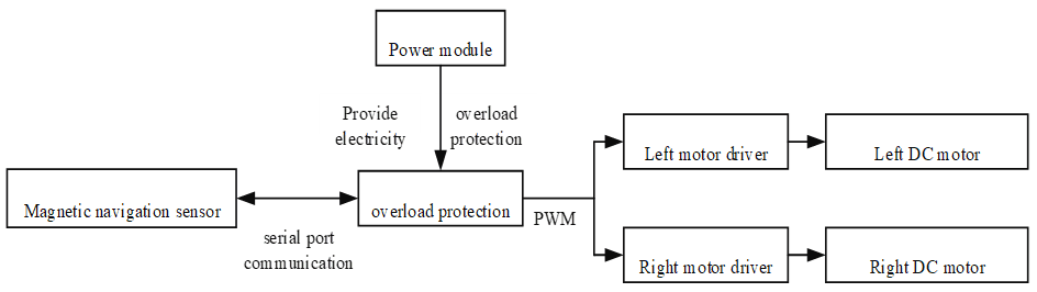
The structure of the worktable is shown in Fig. 1. The control system is mainly composed by a master module, a magnetic navigation module, and a drive module. As shown in Fig. 2, the magnetic navigation module detects the signal of the magnetic strip on the ground. When the sensor senses the magnetic field signal generated by the magnetic strip, it will pass to the main controller module and output the switching signal. The main controller will receive the signal and output the pulse width modulation (PWM) signal to the driver module according to the deviation information of the worktable. It will then change the speed of the left and right motors to realise the deviation correction or steering.

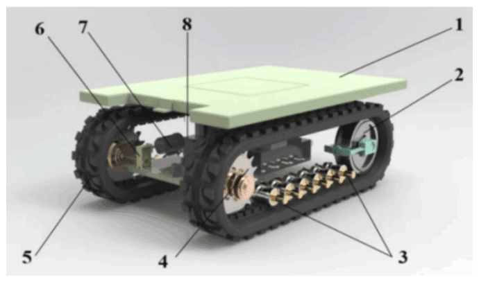
Figure 1 Complete structure of the worktable: 1 – installation platform; 2 – inducer; 3 – supporting wheel; 4 – driving wheel; 5 – rubber track; 6 – reducer; 7 – drive motor; 8 – battery.

Figure 2 Composition of control system.

The core component of the main controller module is the STM32F407VET6 development board. This board adopts the ARM Cortex-M4 core processor, 168 MHz CPU running speed, and 512 KB memory. It supports CAN, SPI, UART, and other communication methods, with a certain amount of storage and memory expansion capability and a high sampling rate. The main controller receives the magnetic navigation signals and outputs PWM signals to the motor driver based on the deviation information of the worktable.

The core of the magnetic navigation module is the magnetic navigation sensor, and the magnetic navigation sensor CCF-NS16-OC is selected. The output method is in the form of OC and N/S detection polarity, with a detection distance of 5–85 mm, a sensitivity of 0.5 mT, and a response speed of 0.1 ms detection magnetism that can be adjusted. The magnetic field detector consists of 16 high-sensitivity Hall magnetic sensors, and the interval of each detection point is 10 mm. The magnetic strip is used as a preset navigation path to achieve the preset path of tracking through the cooperation with the magnetic navigation sensor.

The core component of the drive module is the drive motor. To meet the working requirements, the drive motor needs to have good response performance for the timely adjustment of the left and right drive wheel speeds during the driving of the workbench. It also needs to have high instantaneous power and large starting torque.

After comparison, the YP80B14-48V1.1-1500 DC permanent magnet brushless motor is selected, with a rated torque of 7 N m and a speed of 1500 r min⁻¹. The reducer is YPRV063-20-80B14. The motor driver is YPC600-48V.

3 Establishment of motion model

The coordinate system is established with the preset magnetic navigation path as the reference, and the worktable is considered as a whole to establish the kinematic model, as shown in Fig. 3.

Figure 3 Schematic representation of worktable movement.

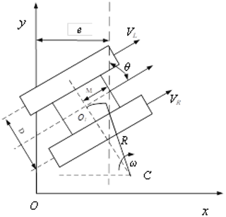
Let the coordinates of the centre O₁ of the worktable at the initial moment T₀ be x₀, y₀, θ₀. The coordinates of the centre O₁ of the worktable are expressed as x_t, y_t, θ_t when T gradually tends to t during the travel of the worktable. Subsequently, the following expressions are given:

$$\begin{array}{}\text{(1)}& {\displaystyle }{x}_t=x_{\mathrm{0}}+\underset{\mathrm{0}}{\overset{t}{\int }}{v}_x\mathrm{d}t=x_{\mathrm{0}}+\underset{\mathrm{0}}{\overset{t}{\int }}v\sin \mathit{\theta }\mathrm{d}t,\text{(2)}& {\displaystyle }{y}_t=y_{\mathrm{0}}+\underset{\mathrm{0}}{\overset{t}{\int }}{v}_{y}vt=y_{\mathrm{0}}+\underset{\mathrm{0}}{\overset{t}{\int }}v\cos \mathit{\theta }\mathrm{d}t,\text{(3)}& {\displaystyle }{\mathit{\theta }}_t={\mathit{\theta }}_{\mathrm{0}}+\underset{\mathrm{0}}{\overset{t}{\int }}\mathit{\omega }\mathrm{d}t,\end{array}$$

where v is the workbench running speed, v_x is the workbench x-directional partial speed, v_y is the workbench y-directional partial speed, ω is the turning angular velocity of the workbench, and θ is the angular deviation of the workbench forward direction from the preset magnetic strip.

The expression of the position deviation value e is

$$\begin{array}{}\text{(4)}& \begin{array}{rl}e& =x_{\mathrm{0}}+\underset{\mathrm{0}}{\overset{t}{\int }}\left[\sin \left({\mathit{\theta }}_{\mathrm{0}}+\underset{\mathrm{0}}{\overset{t}{\int }}{\displaystyle \frac{\mathrm{\Delta }wr}{D}}\mathrm{d}t\right)v\right]\mathrm{d}t,\\ & +M\sin \left({\mathit{\theta }}_{\mathrm{0}}+\underset{\mathrm{0}}{\overset{i}{\int }}{\displaystyle \frac{\mathrm{\Delta }wr}{D}}\mathrm{d}t\right),\end{array}\end{array}$$

where $\mathrm{\Delta }w=w_{\mathrm{L}}-w_{\mathrm{R}}$, w_L is the speed of the left driving wheel, w_R is the speed of the right driving wheel, r is the driving wheel radius, and M is the distance between the centre O₁ of the magnetic navigation sensor and the centre of the worktable.

Assuming that the angular deviation and lateral distance deviation produced by the worktable after normal driving time Δt are Δθ and Δe, respectively, when Δθ tends to 0, the following expressions can be obtained by integrating Δθ and Δe, respectively:

$$\begin{array}{}\text{(5)}& {\displaystyle }\mathrm{d}\mathrm{\Delta }e={\displaystyle \frac{v_{\mathrm{L}}+v_{\mathrm{R}}}{\mathrm{2}D}}\sin \mathit{\theta }\mathrm{d}t,\text{(6)}& {\displaystyle }\mathrm{d}\mathrm{\Delta }\mathit{\theta }={\displaystyle \frac{v_{\mathrm{L}}-v_{\mathrm{R}}}{\mathrm{2}D}}\mathrm{d}t,\end{array}$$

where v_L is the linear velocity of the left track wheel, v_R is the linear velocity of the right track wheel, and D is the distance between the left and right tracks.

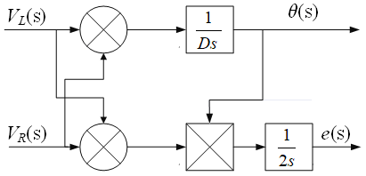
Although the motion system of the worktable is nonlinear, the operating state of the worktable is continuous. The angular deviation θ is very small in the actual normal operation, so we let sinθ=θ, and the following expression can be obtained by the Laplace transform:

$$\begin{array}{}\text{(7)}& {\displaystyle }\mathit{\theta }\left(s\right)={\displaystyle \frac{v_{\mathrm{L}}+v_{\mathrm{R}}}{Ds}},\text{(8)}& {\displaystyle }e\left(s\right)={\displaystyle \frac{v_{\mathrm{L}}+v_{\mathrm{R}}}{\mathrm{2}s}}\mathit{\theta },\end{array}$$

where the relationship between the right and left drive wheel speeds called v_R, v_L, respectively, angular deviation θ, and position deviation e in the operation of the worktable, are given in Eqs. (7) and (8). The real-time adjustment of the left and right drive wheel speeds can effectively complete the adjustment of the worktable's positional state. This include parameters such as driving speed, position deviation, and angle deviation. The kinematic characteristics of the worktable are shown in Fig. 4.

Figure 4 Motion characteristics of workbench.

The workbench adopts a DC brushless motor and a corresponding relationship exists between the armature voltage of the motor and the linear speed of the driving wheel rotation:

$$\begin{array}{}\text{(9)}& {\displaystyle }{v}_{\mathrm{L}}\left(s\right)={\displaystyle \frac{\mathrm{1}}{\mathrm{1}+T_{\mathrm{m}}s}}{U}_{\mathrm{L}}\left(s\right),\text{(10)}& {\displaystyle }{v}_{\mathrm{R}}\left(s\right)={\displaystyle \frac{\mathrm{1}}{\mathrm{1}+T_{\mathrm{m}}s}}{U}_{\mathrm{R}}\left(s\right),\end{array}$$

where U_L(s) is the armature voltage of the left drive motor of the worktable, U_R(s) is the armature voltage of the right drive motor of the worktable, and T_m is the motor response time constant.

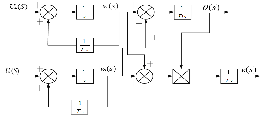
According to Eqs. (7), (8), (9), and (10) and Fig. 4, the dynamic characteristics of the work platform's structure block diagram is established, as shown in Fig. 5.

Figure 5 Motion characteristic structure diagram of workbench.

The dynamic characteristic structure of the worktable is linearised for small deviation. The linear relationship between the voltage increment of the driving motor and the driving lateral deviation during the deflection correction of the worktable is shown in Fig. 6.

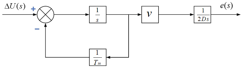
Figure 6 Block diagram of the relationship between voltage increment and operating deviation.

According to Fig. 6, the transfer function of the workbench is given in Eq. (11):

$$\begin{array}{}\text{(11)}& G\left(s\right)={\displaystyle \frac{T_{\mathrm{m}}sv}{\mathrm{2}Ds(T_{\mathrm{m}}s+\mathrm{1})}}.\end{array}$$

4 Design of fuzzy PID controller

4.1 Parameter determination of controller

If the worktable is controlled by the traditional PID algorithm, then the control system will lack flexibility and adaptability, and the anti-interference ability of the system will be poor. Establishing an accurate model is difficult because the motion system of the work platform itself has large uncertainty and nonlinearity, along with the influence of the environment. On the contrary, fuzzy control does not depend on the mathematical model of the object and has better practicality for nonlinear models. Therefore, the study adopts the fuzzy PID control principle to input the deviation quantity e and the deviation rate of change e_c into the PID controller. It forms new control parameters by combining them with the output correction quantity after fuzzy reasoning so as to realise the effective control of the controlled object. It then ensures the realisation of the magnetic navigation function and the optimisation of the performance of the worktable.

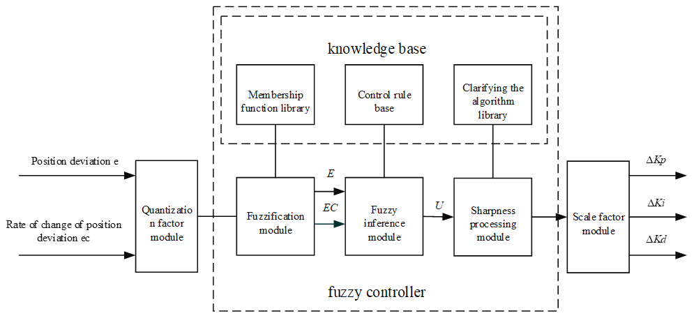
The fuzzy controller designed in the study adopts the structure of two inputs and three outputs, as shown in Fig. 7. The input quantity is the lateral deviation e and deviation rate of change e_c generated during the motion of the worktable. The output quantity is the adjustment quantity of the three parameters of Δk_P, Δk_i, and Δk_d.

Figure 7 Structure block diagram of fuzzy PID controller.

In the fuzzy controller, the shape of the membership function affects the performance of the entire control system. Under normal circumstances, the sharp-shaped membership function can improve the sensitivity of the control system, while the flat-shaped membership function can optimise the stability of the control system. Therefore, considering various factors, The Gaussian membership function is chosen to achieve fuzzification. The basic theoretical domains L of the lateral position deviation e and the rate of change of the lateral position deviation e_c are determined as [$-\mathrm{6},\mathrm{6}$]. Taking the sensitivity and delay characteristics of the system into account, the corresponding fuzzy domains F are set to [$-\mathrm{3},\mathrm{3}$], from which the quantisation factor of the input quantity e and e_c is obtained as in the following Eq. (12):

$$\begin{array}{}\text{(12)}& k_e=k_{e_{\mathrm{c}}}={\displaystyle \frac{max\left(F\right)}{max\left(L\right)}},\end{array}$$

where e is the lateral deviation of the system, e_c is the lateral deviation rate of the system, max(F) is the maximum value of the fuzzy domain F, max(L) is the maximum value of the basic domain L and k_e and $k_{e_{\mathrm{c}}}$ are the quantisation factors of the input quantity e and e_c, respectively. Substituting the values of max(F), max(L) gives $k_e=k_{e_{\mathrm{c}}}=\mathrm{0.5}$.

The fuzzy domains of the three adjustment quantities, Δk_P, Δk_i, and Δk_d are set to [$-\mathrm{0.3},\mathrm{0.3}$], [$-\mathrm{0.06},\mathrm{0.06}$], and [$-\mathrm{3},\mathrm{3}$], respectively. The fuzzy domains of the lateral deviation of the above parameter e, the rate of change of the lateral deviation e_c, and the parameter adjustment Δk_P, Δk_i, and Δk_d can be divided into the following seven quantisation levels, $e=\mathit{\{}\mathrm{NB},\mathrm{NM},\mathrm{NS},\mathrm{ZO},\mathrm{PS},\mathrm{PM},\mathrm{PB}\mathit{\}}$, $e_{\mathrm{c}}=\mathit{\{}\mathrm{NB},\mathrm{NM},\mathrm{NS},\mathrm{ZO},\mathrm{PS},\mathrm{PM},\mathrm{PB}\mathit{\}}$. The specific meanings of the different quantisation levels of the fuzzy domain are shown in Table 1.

Table 1 Specific meanings of different quantisation levels.

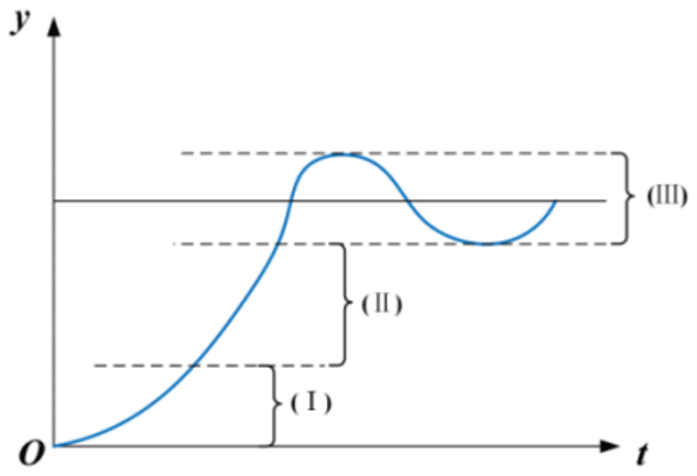
According to the analysis of the output response of the controller adjustment rule, the adjustment principles of the three parameters K_P, K_i, and K_d of the fuzzy PID controller are as follows:

1. When the deviation value is large, the response is in the section I of the curve shown in Fig. 8. At this time, it is necessary to increase k_P and decrease K_d, while making k_i close to 0.

2. When the deviation value and the rate of change are in the middle of the domain, the response is in the section II of the curve shown in Fig. 8. It is necessary to reduce k_P and take the appropriate sizes of k_i and K_d.

3. When the deviation value is small, the response is in the section III of the curve shown in Fig. 8. It is necessary to increase K_P and K_i and take the appropriate size of K_d .

Figure 8 Outputs of the corresponding curve.

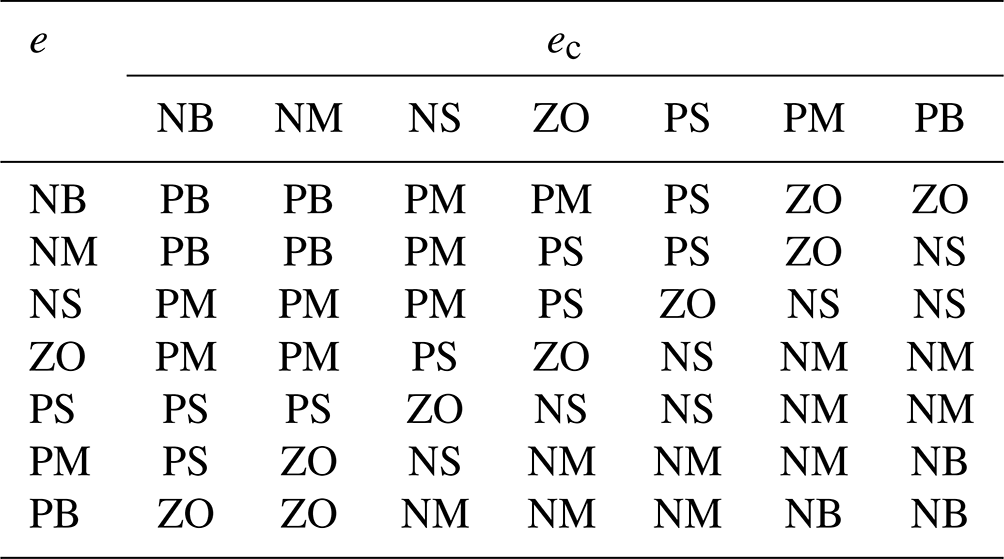
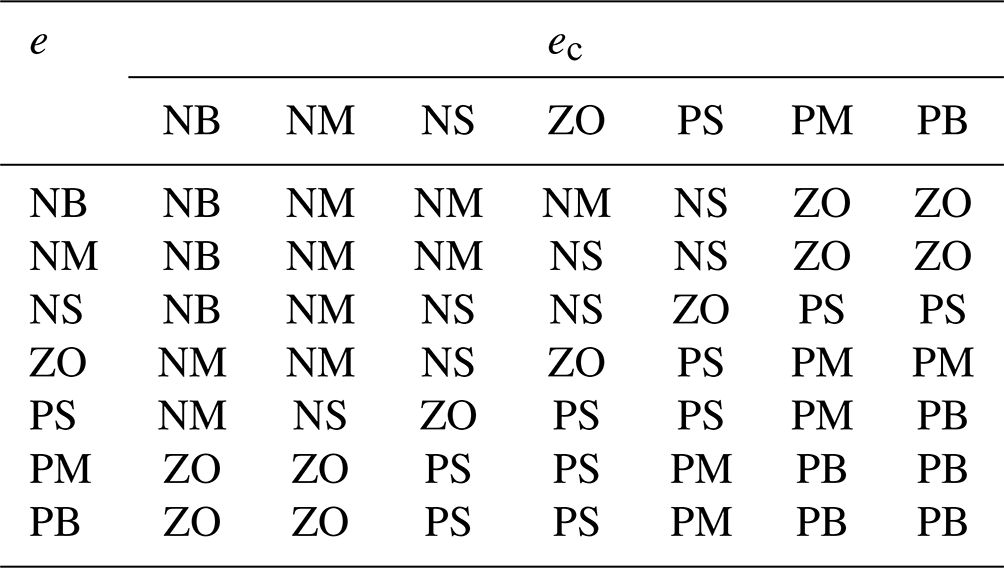
Combined with the actual working situation of the worktable, the fuzzy control rules of ΔK_P, ΔK_i, and ΔK_d are established as shown in Tables 2, 3, and 4.

Table 2 ΔK_P fuzzy control rule table.

Table 3 ΔK_i fuzzy control rule table.

Table 4 ΔK_d fuzzy control rule table.

The control system needs to clarify the linguistically expressed fuzzy control quantity after fuzzy reasoning to obtain the exact quantity. In this study, the chosen method is the centre of gravity method. The defuzzification of the output quantity is realised by cumulatively summing up and averaging each element in the output quantity and its corresponding affiliation. For the discrete domain, the expression is shown in Eq. (13):

$$\begin{array}{}\text{(13)}& z_{\mathrm{0}}={\displaystyle \frac{\sum _{i=\mathrm{1}}^{n}M\left(u_i\right)u_i}{\sum _{i=\mathrm{1}}^{n}M\left(u_i\right)}},\end{array}$$

where z₀ is the exact control quantity, u_i is the element in the fuzzy domain, and M(u_i) is the affiliation value of the fuzzy subset at u_i.

The range of the output quantity after the clarification is usually not the same as the range of the actual domain of the controlled object, so the scaling factor needs to be determined computationally to reasonably scale the processed values. The fuzzy domains of the three adjustment quantities ΔK_P, ΔK_i, and ΔK_d are [$-\mathrm{0.3},\mathrm{0.3}$], [$-\mathrm{0.06},\mathrm{0.06}$], and [$-\mathrm{3},\mathrm{3}$], and the fundamental domains are [$-\mathrm{12},\mathrm{12}$], [$-\mathrm{1.2},\mathrm{1.2}$], and [$-\mathrm{6},\mathrm{6}$], respectively. The scaling factors K_up, K_ui, K_ud for the three adjustment quantities are obtained as follows: $K_{up}=\mathrm{12}/\mathrm{0.3}=\mathrm{40}$, $K_{ui}=\mathrm{1.2}/\mathrm{0.06}=\mathrm{20}$, and $K_{ud}=\mathrm{6}/\mathrm{3}=\mathrm{2}$. This results in the parameter list of the linguistic variables, as shown in Table 5.

Table 5 Parameter list of language variables.

4.2 Simulation of fuzzy PID controller

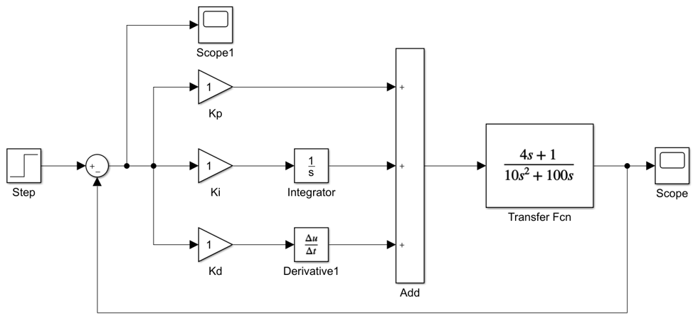
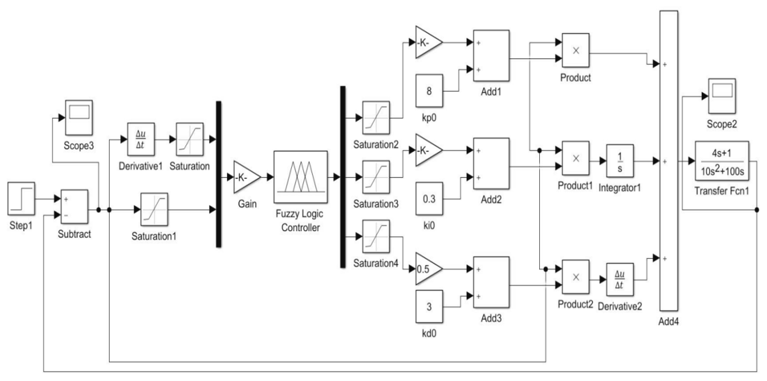
To verify the performance of the designed fuzzy PID controller, simulation analysis is conducted in MATLAB/Simulink. The control effect of the fuzzy controller is analysed by simulation curves. The Simulink block diagram of the conventional PID control algorithm is introduced in the same environment to have an obvious comparison with the conventional PID controller. The focus is on comparing the response ability of both for the same deviation. The Simulink block diagrams of the conventional PID control algorithm and the fuzzy PID control algorithm are shown in Figs. 9 and 10, respectively.

Figure 9 Simulink block diagram construction of conventional PID controller.

Figure 10 Simulink block diagram construction of fuzzy PID controller.

In computer simulation, the worktable is set to travel at 0.4 m s⁻¹; the initial position deviation and angle deviation are 3 cm and 0^∘, respectively; and the sampling time is 0.02 s. At this time, the system has a transfer function, as shown in Eq. (14):

$$\begin{array}{}\text{(14)}& z_{\mathrm{0}}={\displaystyle \frac{\mathrm{4}s+\mathrm{1}}{\mathrm{10}{s}^{\mathrm{2}}+\mathrm{100}s}}.\end{array}$$

With the above parameter settings, the output responses of different controllers are run separately under the initial deviation signals, as shown in Fig. 11.

Figure 11 Comparison of simulation results.

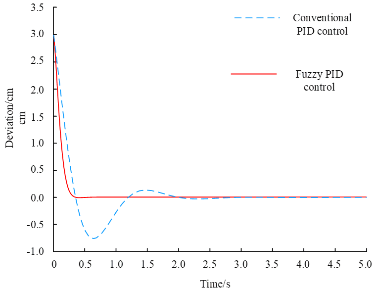
The analysis shows that the fuzzy PID algorithm can correct the deviation in approximately 0.5 s, and the correction is rapid. There is no fluctuation during correction, but the whole correction process of the conventional PID controller needs to go through 3–4 times of repeated oscillation. The amplitude gradually decreases, and finally the correction of deviation is completed in 3–3.5 s. The fuzzy controller designed in the study has a fast response, less fluctuation, and smooth change process. The entire system presents good stability.

5 Experimental verification analysis

5.1 Experimental design

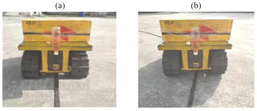
To verify the reliability and smoothness of the designed system, the error analysis of the designed motion control system is required. The magnetic strips are laid on the hard outdoor concrete surface as the experimental environment. The greenhouse magnetic navigation AGV table prototype based on fuzzy PID control is used as the experimental object. The straight magnetic strips and curved magnetic strips are laid on the ground as the navigation path. The centre of the magnetic navigation sensor, the centre of the vehicle body, and the centre of the magnetic strips are on the same surface. The bottle with the coloured solution is installed in the centre of the back-end of the worktable. The actual error of the table is defined by recording the lateral distance between the centre of the dripping solution and the centre line of the magnetic strip using the trickle method. The performance of the system is analysed by measuring the actual error in the straight running case and the curved driving case as shown in Fig. 12.

Figure 12 Two driving conditions of AGV: (a) straight driving and (b) curve driving.

5.2 Test process and results

5.2.1 Straight driving test

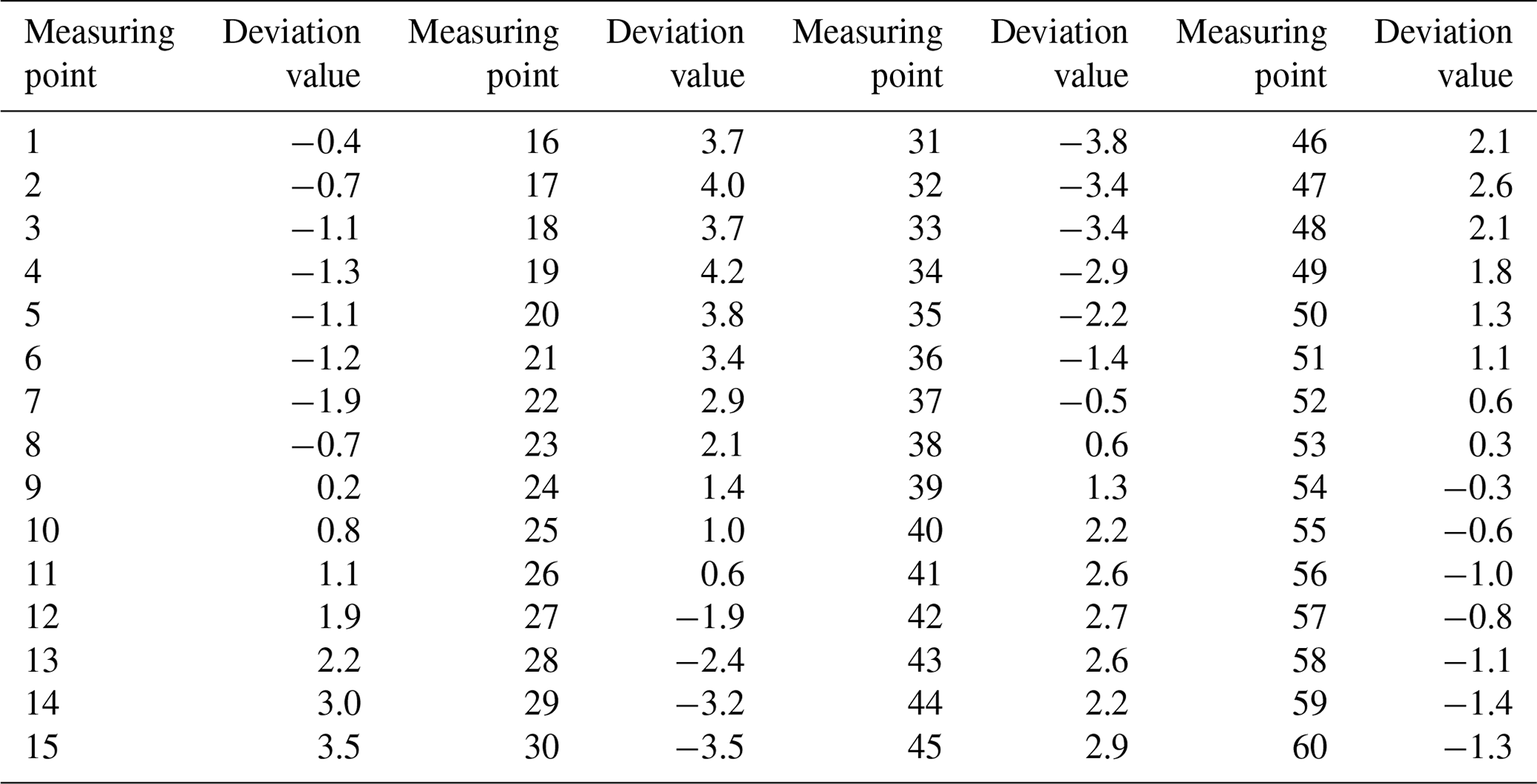
The platform starts to drive in a straight magnetic strip of 8 m at a speed of 0.6 m s⁻¹. The lateral distance between the centre of the dripping solution and the centre line of the magnetic strip is measured every 10 cm. The left deviation is considered to be negative and the right deviation is considered to be positive. The absolute values of the deviations obtained from the three tests are summed and averaged as the deviation value. In addition, if the number of left deviations is greater than the number of right deviations in the three tests, the deviation is considered to be left deviation, and vice versa. A total of 60 sets of test data are calculated, as shown in Table 6.

Table 6 Test data of straight running measurement (average).

Table 7 Curve operation measurement test data (average).

5.2.2 Curve driving test

The same worktable starts to drive with the speed of 0.6 m s⁻¹ and conducts three tests. The radius of the arc is gradually increased from 2 to 6 m. When the radius of the arc is less than 6 m, the worktable will be out of the preset magnetic strip trajectory. To ensure smooth driving, a certain length of straight magnetic strip is added to each part of the incoming and outgoing curves. The lateral distance between the centre of the dripping solution and the centre line of the magnetic strip is measured every 10 cm, with the left deviation being negative and the right deviation being positive. In addition, if the number of left deviations is greater than the number of right deviations in the three tests, the deviation is considered to be a left deviation, and vice versa. Sixty sets of test data are calculated, as shown in Table 7.

The analysis of the 60 measured lateral deviations in Tables 6 and 7 shows that the maximum left deviation is roughly 1.9 cm and the maximum right deviation is nearly 1.1 cm during the three tests of the worktable's straight run. The overall deviation is controlled in the range of ±2.5 cm. In the same way, the maximum left deviation is approximately 3.8 cm, and the maximum right deviation is around 4.2 cm during the bending operation of the worktable. The overall deviation is controlled within ±4.5 cm. This outcome shows that the worktable still has good trajectory navigation ability for the preset magnetic stripe during the bending operation.

6 Conclusion

The following conclusions can be drawn from the tests conducted on the outdoor hard ground in the straight and curved paths.

1. The maximum lateral deviation of the prototype is 1.9 cm after walking for 5 m in the case of a straight line, and 4.2 cm in the case of a curve and 90^∘. The experimental results show that the navigation based on magnetic stripe can be carried out according to the preset path. In addition, the navigation accuracy can meet the general operation requirements.

2. During the test, the vehicle moves smoothly and reacts rapidly, and there is no obvious vibration and delay in the body movement, indicating the stability and reliability of the movement in the straight line. When turning, the reaction is rapid, and the correction is realised within a short distance without deviating from the course. The experiment verifies the stability and reliability of the designed fuzzy PID control.

Compared with other navigation methods, the magnetic navigation method based on fuzzy PID control has low cost and smooth and reliable motion. Moreover, the accuracy error can meet the requirements of general agricultural operations.