the Creative Commons Attribution 4.0 License.
the Creative Commons Attribution 4.0 License.
 | 28 Sep 2022
TGA-based solutions map method for four-position synthesis of planar 4R linkage
Yehui Zhao
Lijun Xue
Fanglei Zou
Yue Song
Hongjian Zhang
In this study, the authors propose a solutions map based on a telomere genetic algorithm (TGA) to improve the efficiency of 4R-linkage synthesis. First, the points on the center curve are obtained by using projective geometry, and those of the circle curve are obtained by vector elimination. Second, the definition of the linkage type, assessment of linkage performance, and a method to identify defects in the linkage are introduced. Third, the solutions map method is proposed that can map the linkage solutions obtained by all combinations of the points on the center curve to a 3D color-coded surface to represent the distribution of solutions with different attributes of linkages in the solution domain. Fourth, we use the proposed telomere operator and pseudo-histogram method to improve the traditional genetic algorithm, and expand the domain of solutions of the solutions map by using the TGA. Finally, the linkage synthesis software BurLink is developed based on the solutions map method. The results show that the TGA-based solutions map can quickly locate the required 4R-linkage solution in the solution domain, and provides engineers with more candidate solutions than traditional methods.
- Article
(3827 KB) - Full-text XML
- BibTeX
- EndNote


The positional synthesis of the 4R linkage is the inverse calculation of its kinematic analysis, i.e., to calculate the parameters of linkage according to several specified positions of the coupler. It is widely used in engineering. The Burmester theory (Cera and Pennestrì, 2018, 2019; Shirazi, 2007) points out that at most, five accurate positions can be specified in positional synthesis. Because the number of candidate solutions for a five-position synthesis problem is no more than six, this can easily lead to a situation where no viable solution is available, and this renders four-position synthesis more practical for use in engineering. According to the Burmester theory, any two center points yield a linkage solution such that the four-position synthesis problem has ∞2 solutions in theory. Although there are many combinations of center points, most solutions involve defects in the circuit, branch, or order (Baskar and Bandyopadhyay, 2019; Singh et al., 2017; Tipparthi and Larochelle, 2011), which requires engineers to often spend weeks or even longer on repeated calculations and analyses to obtain satisfactory linkage solutions. Therefore, it is important to solve the problem of the poor efficiency of four-position synthesis. The goal of this study is to improve the efficiency of synthesis through a computer-aided method of synthesis. The theories of synthesis and analysis used here are introduced in Sects. 2 and 3, respectively, and the corresponding methods and software are provided in Sects. 4 and 5, respectively. The main conclusions are summarized in Sect. 6.
It is easy to determine that three factors affect the synthesis efficiency of the 4R linkage: (i) the lack of effective methods for identifying defective solutions, (ii) the blindness of the selection of points on the center curve, and (iii) the absence of a viable solution owing to the small number of available solutions in the domain. Previous studies have thus focused on these issues. To identify defective solutions, Filemon (1972) used the intersection of opposite sides of opposite pole quadrilaterals to divide the center curve into six segments, and found that the 4R linkage formed by the two center points in the same segment had the same order of couplers. Similarly, Waldron and Strong (1978), and Gupta and Beloiu (1998) used region segmentation technology with the Burmester curve to identify defects in the branch and circuit of the linkage. Based on the same technology, Sun and Waldron (1981) controlled the transmission angle of the linkage within a prescribed range while realizing defect-free linkage synthesis. The most effective method to mitigate the blindness of selection of points on the center curve involves visualizing the solution domain. McCarthy (2013) and Ruth and McCarthy (1999) proposed the type map method in their synthesis software Sphinx (the latest version is SphinxPC). It can build a mapping between the combination of points on the center curve and the attributes of linkage type. After Sphinx, the analysis of the solution domain has been extended gradually to other fields of linkage synthesis. In addition to the early software for linkage synthesis Lincages (Erdman and Loftness, 2005), Cao and Han (2020), Han and Cao (2018), and Liu and Han (2021) recently used solution-domain analysis to solve the problems of the synthesis of spatial linkages, such as RCCC, 1CS-4SS, and HCCC. In case no feasible solution is available, approximate motion synthesis expands the solution domain by introducing errors that can ensure the existence of the solution at the expense of accuracy. Many studies have contributed to this field. Gogate and Matekar (2012) used the evolutionary algorithm for the approximate motion synthesis of the 4R linkage and then applied this method to the synthesis of the Watt-I six-link mechanism (Gogate and Matekar, 2014). Sundram and Larochelle (2015) solved the mixed exact–approximate synthesis problem based on the constrained nonlinear optimization toolbox of MATLAB. Similarly, Ravani and Roth (1983) used kinematic mapping to transform the problem of approximate motion synthesis into that of curve fitting in the image space, while Ge et al. (2017) reduced this problem to that of finding a G-manifold that can best fit points in the image in the least-squares sense. Although previous studies in different fields have solved one of the above three problems that lead to poor efficiency of synthesis, they cannot solve all three at the same time. Integrating different methods may be an effective approach to solving all of these problems.
The region-based segmentation technology for the Burmester curve attempts to remove the points on the center curve or those in the circle curve that may cause defects before obtaining the linkage solution. However, this technology cannot accurately distinguish between defective and non-defective solutions, and excludes part of the reasonable linkage solutions while excluding defective solutions. This significantly reduces the chance of finding feasible solutions. By contrast, the type map method carries out defect discrimination once the parameters of linkage have been determined; thus, it has a higher accuracy than region-based segmentation technology. Moreover, type map can visualize the solution domain so that engineers can select the center points according to the type of linkage, thereby avoiding the blindness of the process of linkage synthesis. However, the number of candidate solutions provided by type map is usually too small to meet engineering needs. Approximate and accurate position synthesis are subjects in different fields of research. They can be used to solve the four-position synthesis problem and usually obtain only one linkage solution per calculation, but this solution is obtained by active search in the solution domain through an optimization algorithm. Theoretically, a satisfactory solution can be obtained directly by adding a sufficient number of constraints to the optimization model, but this is not feasible in many cases: a mathematical model with many constraints is too complex to establish, and strong constraints may also cause the optimization algorithm to fail to converge. To sum up, the type map method can completely replace the traditional synthesis method based on region segmentation technology. Therefore, only the possibility of its integration with the problem of approximate-motion synthesis needs to be considered. To solve the above three problems that affect the efficiency of synthesis, the concept of error in approximate-motion synthesis is introduced to accurate-position synthesis in this study to simultaneously expand and visualize the solution domain. Specifically, a solutions map method based on a telomere genetic algorithm (TGA) that can analyze and expand the solution domain is proposed in this study.
2.1 Generation of center curve
As shown in Fig. 1, the purpose of this study is to design a 4R linkage, A0A1B1B0, so that a point E on the coupler AB can pass through four specified positions in sequence. The specified positions of the coupler are defined in the planar rectangular coordinate system and denoted by P (xP, yP, δ), where xP and yP are the abscissa and the ordinate of point P, respectively, and δ is the angle of rotation of the coupler. According to the Burmester theory, the key to solving this problem is to calculate the curves of the center and circle. Because the center curve directly reflects the positions of the fixed hinge A0 and B0, it should be generated first.
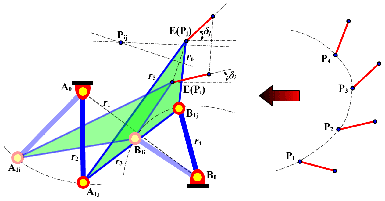
For any two positions of the coupler Pi (, , δi) and Pj (, , δj), the pole point pij (, ) can be calculated by the following equation:
when the origin of the coordinate system moves to pole point p12, the equation of the Burmester center curve C1234 can be expressed as follows (Zhang, 1983):
where
The center curve C1234 is a third-order circular point curve. According to projective geometry (Jin and Shi, 1991), the curve usually has a real focus, and the solution of Eq. (2) can then be expressed as follows:
where σ is the input variable, and the other variables are defined as:
Note that the sign of γ is “+” only when j2≥0.
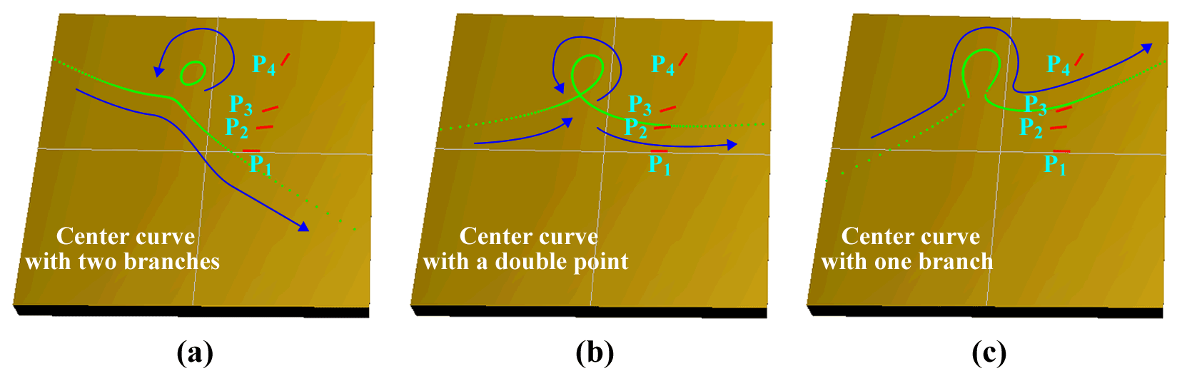
In this case, the shape of the center curve depends on the value of τ:
If τ>0, C1234 is a non-closed curve, if τ=0, C1234 is a non-closed curve with one coincident point, and if τ<0, C1234 is divided into a non-closed curve and an elliptic curve. To control the distribution density of the generated Burmester center points, the input variable σ can be parameterized as follows:
where α and k are constants.
Note that the order of tan(φ) cannot be even. This leads to , such that one part of the center curve is repeatedly calculated and the other part is lost.
To facilitate programming, the range of values of φ under any condition is set to in this study. The equations based on this are shown in Table 1, and are used to generate each part of the center curve in turn to ensure that points of each part of the curve are connected from head to tail without jumps. Once all points on the center curve have been calculated, it is necessary to preprocess each point. For example, points on the center curve outside the set area are eliminated according to their coordinates, and center points with too small a spacing between them are eliminated according to the Euclidean distance between adjacent points. Three typical center curves generated by a computer program based on the above method are shown in Fig. 2.

2.2 Computation of points on the circle curve
Considering that it is difficult to generate the circle curve from the center curve by using the geometric method, the traditional vector elimination method (Liang and Chen, 1993) is improved so that it can generate the circle curve according to the coordinates of the points on the center curve. According to this method, the RR links (i.e., A0A1−A1E in Fig. 1) satisfy the following equation in motion:
where δ0 is the initial angle of the link A1E and . We define the following:
By substituting the above formulae into Eq. (8), the following equation is obtained after simplification:
After the numerical computation of matrix inversion, the above equation is transformed into
where Ak, Bk, and Ck are elements of the matrix.
In previous research (Liang and Chen, 1993; Zhao, 2009), Eq. (11) has been decomposed into several sub-formulae that can be merged into a high-order equation with only one variable by elimination:
where E1−E4 are coefficients related to Ak, Bk, and Ck.
After solving the equation by dichotomy or Newton's iterative method, the values of all variables can be obtained in a step-by-step manner based on the relationships between them. Note that because it is difficult to unify the symbolic definition in Fig. 1 and the algebraic definition in Eq. (9), there are significant differences between Eqs. (11) and (12) as derived in the literature, but the principle of vector elimination considered is consistent. Although this method can offer a direct solution for the coordinates of points on the center curve and the circle curve, rectangular coordinates that cannot reflect the trend of the Burmester curve are used to generate the points on the center curve. For example, this method needs to first specify the abscissa of the point on the center curve, where this coordinate can be taken arbitrarily on the plane and its value is independent of the shape of the center curve. It is thus difficult to parameterize the calculation process and avoid jumps when the point on the center curve is generated. This is also why we use the projective geometry method to calculate the coordinates of the point on the center curve. As the center curve has been generated, the vector elimination method is modified in this study. The improved solution process is as follows (Eqs. 13–16):
The following equation is equivalent to Eq. (11):
According to the second and third sub-formulae of Eq. (13), the expressions containing ϑ0 and ϑ1 are obtained as follows:
Further, ϑ0 and ϑ1 are obtained as follows:
Once the coordinates of point A0(xA0, yA0), i.e., the Burmester center point, have been determined, ϑ0, ϑ1, and ϑ3 (=yA0, see Eq. 9) can be solved. By substituting ϑ0 and ϑ1 into the expressions of Eq. (9), r5 and r2 can be written as follows:
where ϑ2 is given by the first sub-formula of Eq. (13).
When the coordinates of points A0 and Pi as well as the link lengths r2 and r5 are known, the coordinates of the point in the circle curve at position i (i= 1,2,3,4) can be calculated as (uw1−vw2, uw2+vw1) (Liang and Chen, 1993), where
Note that the variable v has two solutions. For the correct solution, the rotational angle of the link A1E should be equal to δ0+Δδi. The solution process does not involve the solution of the higher-order equation.
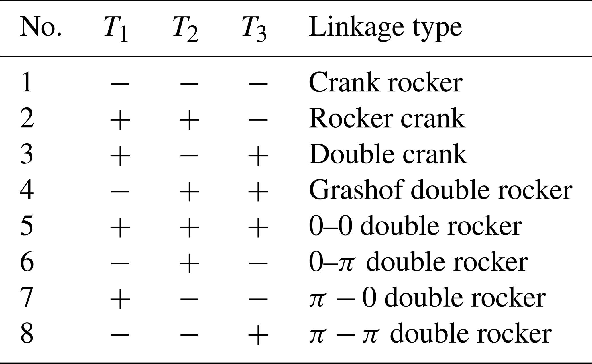
3.1 Linkage type classification
According to the method proposed by Martin and Murray (2002), the 4R linkage can be classified into eight types based on the signs of T1, T2, and T3, as shown in Table 2, where
3.2 Performance evaluation of linkage
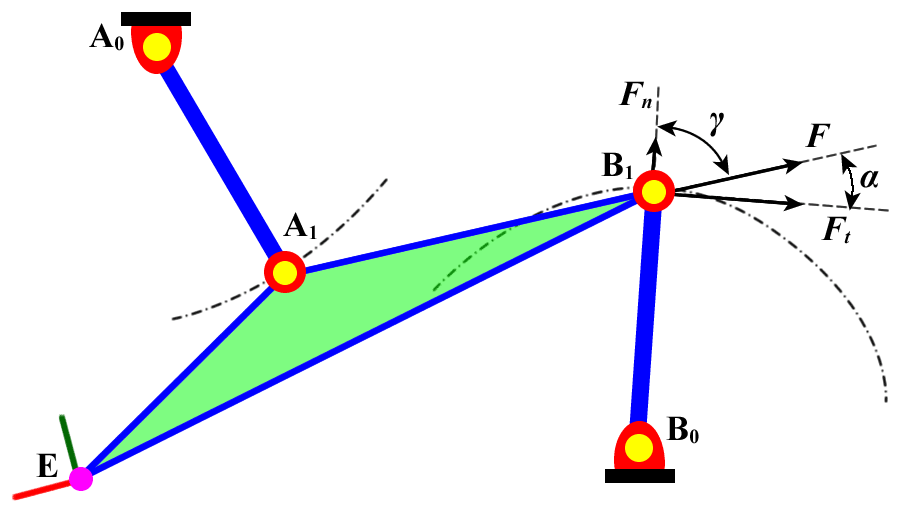
As a discontinuous attribute, the linkage type is often not the only objective of linkage synthesis. It is thus also necessary to consider the values of continuous attributes, such as the link length, transmission angle, acceleration, and force, or their weighted values in the design of the linkage mechanism (Jia et al., 2021; Trejo et al., 2015; Wilhelm et al., 2017). For convenience of understanding, this study takes the transmission angle as the index to assess the performance of the linkage. As shown in Fig. 3, if the mass of each link and the friction of the revolute joint are neglected, the coupler A1B1 becomes a two-force link, and the acute angle γ between links A1B1 and B0B1 is the transmission angle. The larger the angle γ is, the greater is the force Ft of the driving force F in the direction of its velocity, and the better is the transmission performance of the 4R linkage. Therefore, when the coupler is in the four given positions, its minimum transmission angle γmin can be used as an index for the evaluation of the transmission-related performance of the 4R linkage.
3.3 Defect discrimination
For each 4R linkage synthesized according to the Burmester theory, we need to discriminate among three kinds of defects, i.e., defects in the circuit, branch, and order, as shown in Fig. 4.
-
Identifying circuit defects. If the driving link A0Ai is not fully rotatable, its range of motion is divided into n sectors based on the limited positions; see Fig. 4a. If the rotation angles of the driving link corresponding to the specified positions of the coupler are in different sectors, the 4R linkage has a circuit defect. In this case, the angles of rotation of the driving link at the limited positions () and the specified positions () should be calculated:
and
Because the domain of definition of the arccosine function is , the number of solutions of in Eq. (19) may be zero, two, or four. There will be no circuit defect in the linkage if all four angles are located in the same sector defined by .
-
Identifying branch defects. As shown in Fig. 4b, the coupler of the 4R linkage usually has two forms of assembly, i.e., A0A1B1(1)B0 and A0A1B1(2)B0. It is difficult for the coupler of the 4R linkage to move from one form to another without jamming. If the planar 4R linkage is placed in the X–Y plane of the 3D coordinate system O-XYZ, the following equation can be used to identify branch defects:
Only if all the four components of the z axis of Vi (i.e., zv) have the same sign (“+” or “−”) when the driving link is located at the specified positions of the coupler, the linkage solution is valid such that it does not contain a branch defect.
-
Identifying order defects. If the driving link of the 4R linkage cannot pass through the four specified positions in the order “1-2-3-4,” it has an order defect. If the driving link is fully rotatable, the order “1-2-3-4” is equivalent to the orders “2-3-4-1,” “3-4-1-2,” “4-1-2-3,” “4-3-2-1,” “3-2-1-4,” “2-1-4-3,” and “1-4-3-2.” The defect-free linkage satisfies φ12<φ13<φ14 or φ12>φ13>φ14, where is the angle of rotation of the driving link when it rotates from position 1 to position i in the anti-clockwise direction. If the driving link is partly rotatable, see Fig. 4c, only “1-2-3-4” and “4-3-2-1” are valid orders because the driving link cannot move from one circuit to another. In this case, the rotational angles of the driving link need to satisfy the condition φt2<φt3<φt4 or φt2>φt3>φt4, where φti is the angle of rotation of the driving link when it rotates from any limited position to the specified position i in the anti-clockwise direction.
-
Organizational rules. When circuit defects occur, the coupler link cannot pass through any of the four specified positions in any condition; when branch defects occur, it cannot pass through the four specified positions without external intervention; when order defects occur, the coupler link can pass through four specified positions but in the wrong order. Therefore, circuit defects are more severe than branch defects, which are more severe than order defects. To reduce the amount of requisite calculation, we stipulate that if a linkage has circuit defects, the programs no longer continue to identify its branch and order defects, and if the linkage has branch defects, the programs no longer continue to identify its order defects.
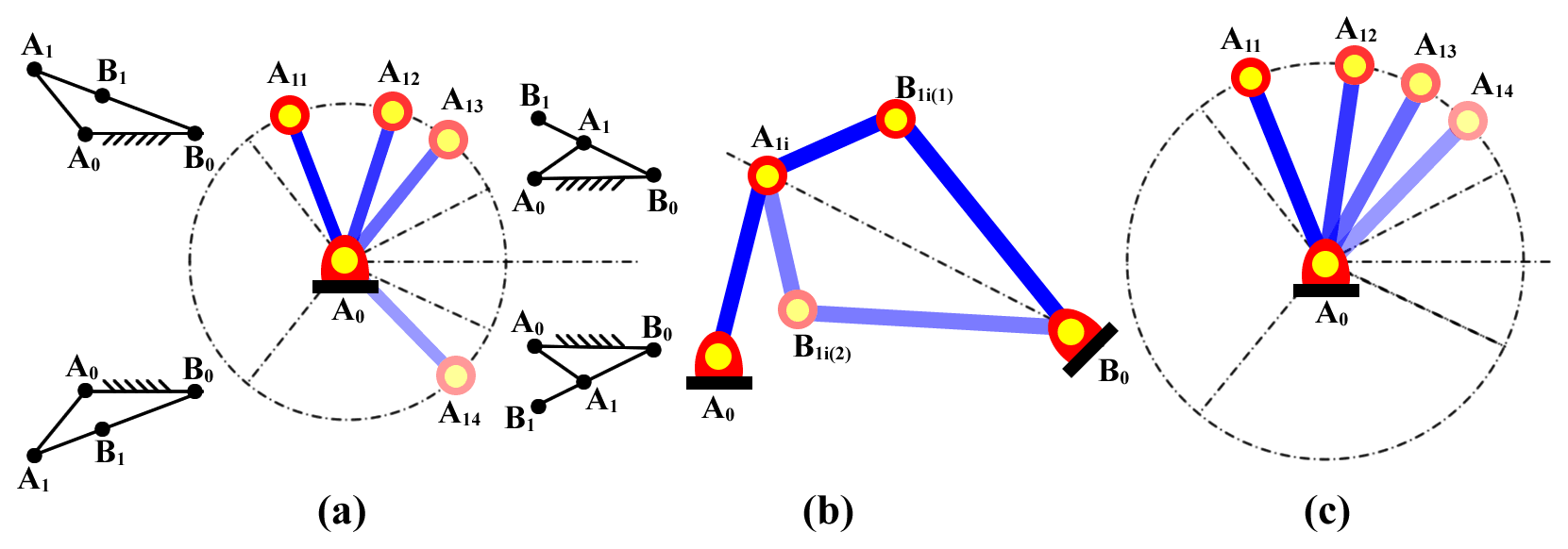
Figure 4Linkage defects in the circuit, branch, and order. (a) Circuit defect. (b) Branch defect. (c) Order defect.
4.1 Principle of solutions map method
The principle of the solutions map proposed in this paper is to map all linkage solutions to a 3D color-coded surface based on linkage type to visualize the distribution of the solutions. There are three steps to generate the solutions map:
-
Generation of Burmester curve. By using projective geometry, N center points can be obtained when the parameter φ changes from to (Sect. 2.1). Note that the number of center points N* is usually less than N because of the preprocessing of the center points. For example, center points beyond the designated area or those with spacing that is too small between them should be excluded. Of course, designers can also adjust the distribution of the center points by changing the value of α or k in Eq. (7). After pretreatment, each center point is assigned a unique index (from 1 to N*) for subsequent calculation. Finally, for each center point, four circle points corresponding to the four specified positions are calculated (Sect. 2.2).
-
Generation of type map. According to the Burmester theory, a solution of the 4R linkage for four specified positions can be determined by any two center points and the corresponding circle points. To describe the distribution of the solution, the x axis and y axis of the rectangular coordinate system are both divided into N* parts to form a grid array of size . If i and jϵN* are defined, the grid coordinates (i, j) represent the linkage solution obtained by combining the center points i and j. For each linkage solution, it is necessary to calculate the linkage type (Sect. 3.1) and fill the grid (i, j) with the color corresponding to it, as shown in Table 3.
-
Generation of solutions map. In total, nine linkage types can be color-coded when the types of defective linkages are considered. To describe the continuously changing attributes of the linkages, type map can be placed in the X–Y plane of the 3D coordinate system. Then, the z-axis of the coordinate system can be used to express the attributes of the linkage introduced in Sect. 3.2. For example, given the task of position synthesis shown in Table 4, the solutions map generated according to the above steps is shown in Fig. 5.
The solutions map consists of the following parts:
- a.
Mountain range. The surface of the solutions map is shaped like a mountain, and any point on the mountain corresponds to a synthesis-based solution of the 4R linkage for the four specified coupler positions. In addition, the color and height of points on the mountain represent the type and performance of the linkage solution, respectively.
- b.
Sea level. There is a sea-like plane across the mountain range that can move up and down along its height (i.e., the z axis of the coordinate system) of the solutions map. The height of the sea level represents the performance of the linkage solution, i.e., the solution corresponding to the mountain part above the sea level is better than the part below it. With a rise in the sea level, the linkage solution with poor performance is submerged.
- c.
Buoy. The buoy is a location tool used to select a linkage solution from the solutions map. It can move freely in the X–Y plane, and its intersection with the mountain range corresponds to a linkage solution.
The method proposed here, based on the solutions map, has the characteristics of a geographical map. The concept of the raster and layer in the Geographic Information System (GIS) can thus be used to organize the data. Raster data consist of location and attribute data. As shown in Fig. 6, any grid in the solutions map is located by its row and column numbers, and corresponds to a linkage solution. As mentioned before, the row and column numbers are index numbers of points on the center curve. Based on this, the attributes of the solutions map can be divided into two types: discontinuous attributes (such as linkage and defect types) and continuous attributes (such as link length, transmission angle, acceleration, force, or their weighted values). Discontinuous data consist of a finite number of values that can be enumerated, and the values of continuous data are arbitrary within a certain range. Each discontinuous attribute is stored in the corresponding layer through the matrix, and elements of the matrix are represented by color codes corresponding to the attribute values. Continuous attributes are also stored in a layer through the matrix, and the elemental value of the matrix is the normalized performance index of the linkage. The discontinuous attributes can be represented by type map while the continuous attributes can be represented by the elevation map. The solutions map can be obtained by superimposing the two maps. Introducing the concept of the layer not only facilitates data management, but also makes the attributes of solutions map easy to query.
- a.
-
Solution selection. Defective solutions in the solutions map can be marked with a specific color (such as white), and solutions that yield poor performance (such as the solution with the minimum transmission angle γmin<20∘ at the four given positions) can be excluded by moving the sea level so that the area of the feasible solution in the solutions map can be located. Consider the position synthesis task shown in Table 4 as an example. Under the guidance of the color code of the solutions map, three groups of linkage solutions of different types can be selected by moving the buoy, as shown in Fig. 7 and Table 5.

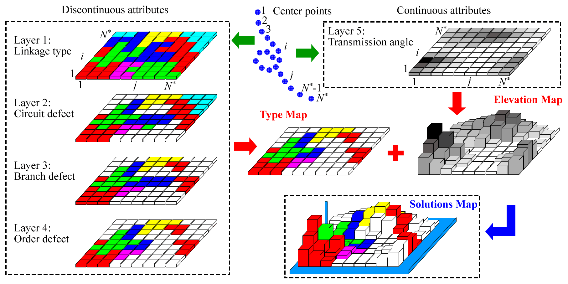
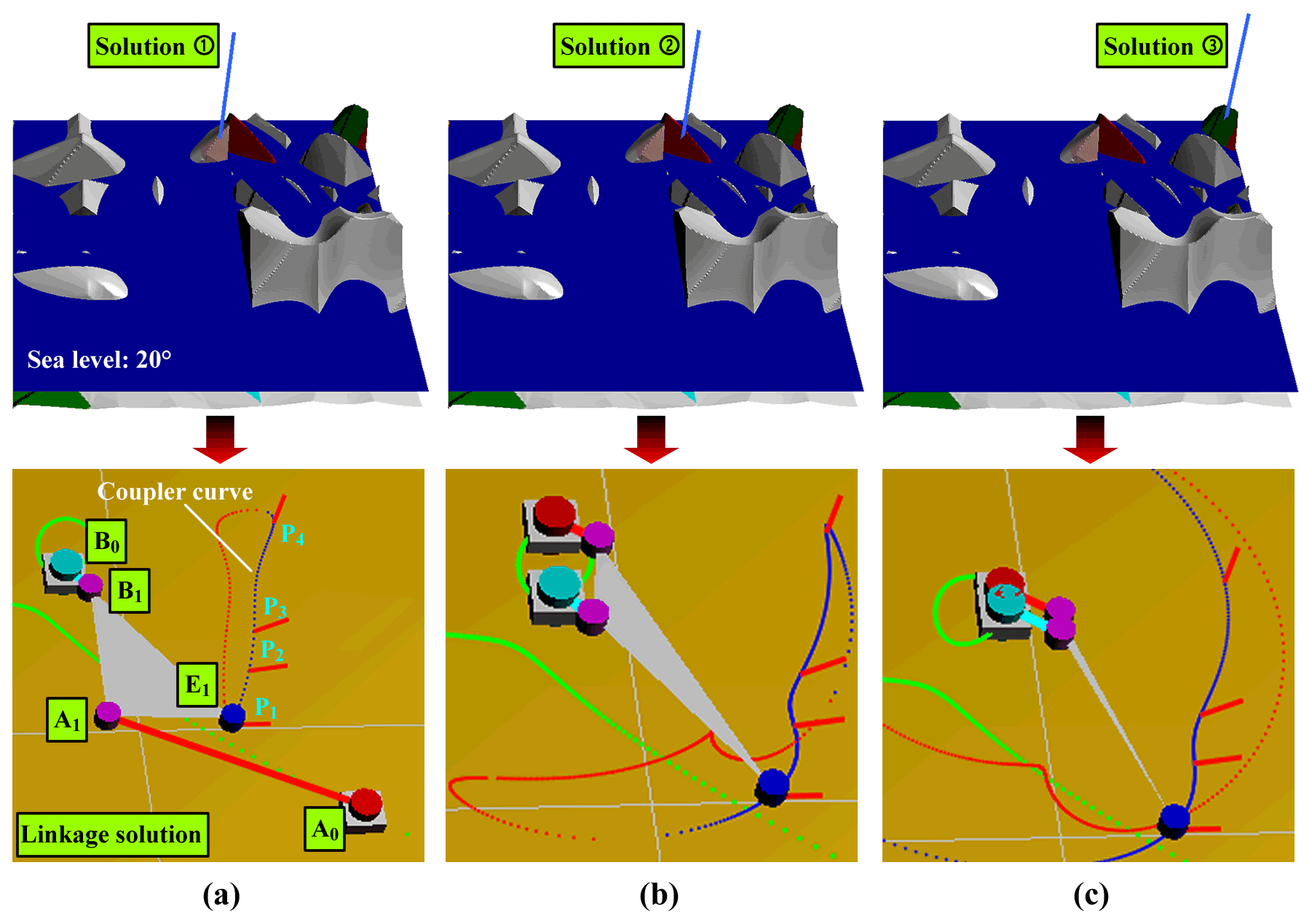
Figure 7Linkage solutions obtained from the solutions map. (a) Solution 1 (0−π double rocker). (b) Solution 2 (π−0 double rocker). (c) Solution 3 (double crank).
Table 5Coordinate-related information of the linkage solutions.

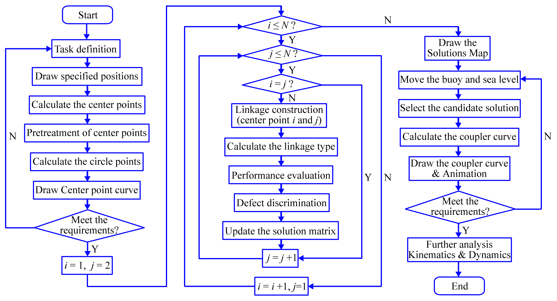
The flowchart of the solutions map method is shown in Fig. 8. In view of the limitations of space, the generation of the coupler curve and the kinematic and dynamic analyses of the linkage are not the main contents of this paper, and are thus not discussed here.
4.2 Problems in basic solutions map
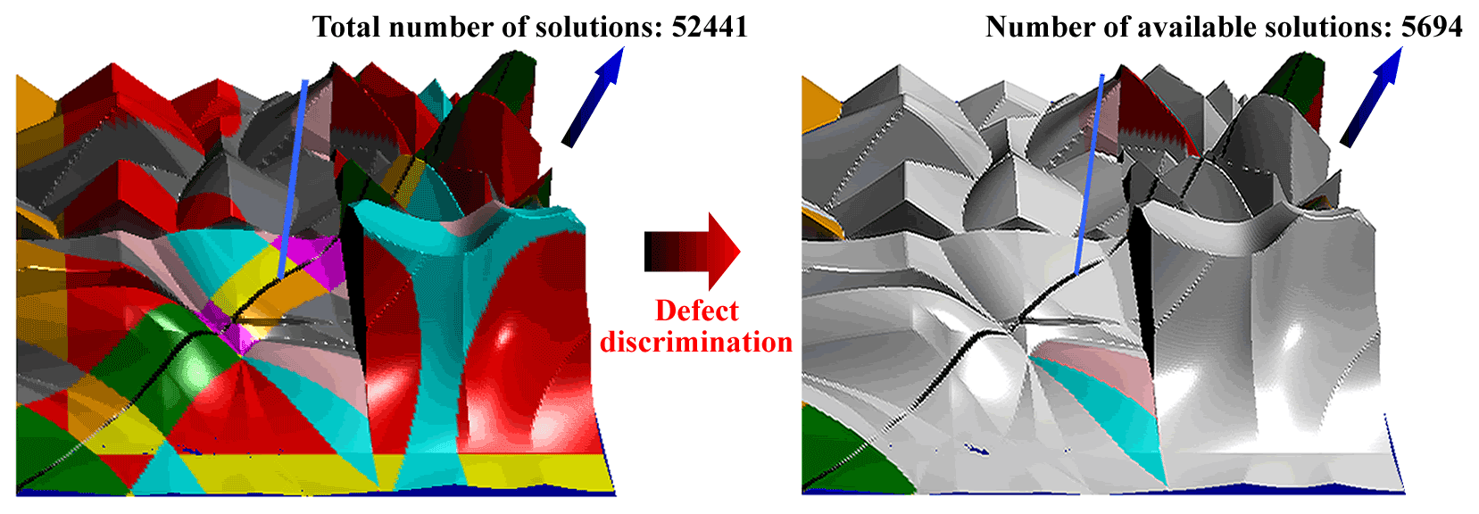
Although the solutions map can quickly locate the required types of linkage solutions and greatly improve the efficiency of synthesis, most 4R linkages synthesized based on the Burmester theory have kinematic defects, where this limits the number of available solutions. In many extreme cases, the given task of position synthesis has no solution. Consider the synthesis task given in Table 4 as an example. After excluding various defective solutions, the number of available solutions in the solutions map is 5694, accounting for only 10.86 % of the total number of solutions, 52 441, as shown in Fig. 9. Note that the solutions in the same region of the solutions map are usually highly similar, which renders options that are very limited. Therefore, it is necessary to expand the solution domain to improve the probability of obtaining feasible solutions.
5.1 Optimization model
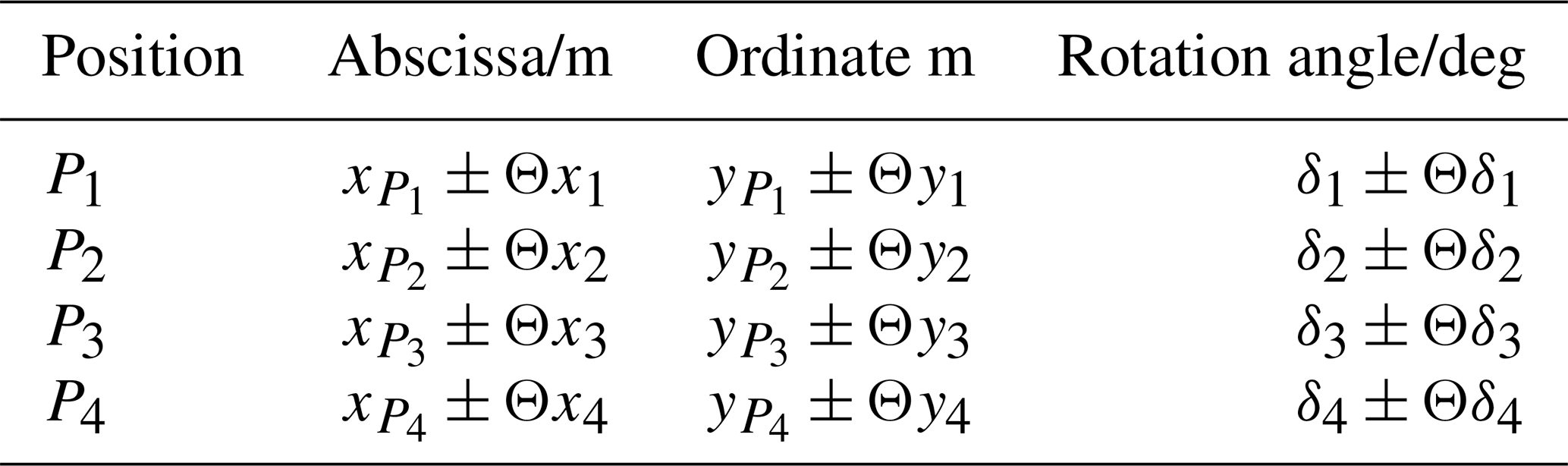
In the context of the problem of approximate motion synthesis, the coupler curve of the 4R linkage only needs to pass approximately through the given four positions. Similarly, although accurate positional information needs to be specified in position synthesis, it is only needed for calculation. In engineering applications, errors are usually allowed in some given positions P (xP, yP, δ). For example, in the design of the material-handling mechanism, only the accuracy of the starting and final positions of the manipulator need to be considered, and the two middle positions are only set to avoid obstacles such that errors in the middle positions are allowable. Similar examples are common, where this blurs the boundary between accurate position synthesis and approximate motion synthesis. Note that accurate position synthesis involves solving specific engineering problems. If the problem itself allows for the existence of errors, it is feasible to expand the solution domain by introducing errors, without caring about whether the problem has been transformed into that of approximate motion synthesis. For convenience of expression, the ranges of errors of xP, yP, and δ are denoted by ±Θx, ±Θy, and ±Θδ, respectively, as shown in Table 6.
When the positional information changes within the allowable range of error, a solutions map with different proportions of the feasible solutions can be obtained to expand the solution domain. This is a typical optimization problem, and its mathematical model can be described as follows:
where X is the solution vector, and its elements consists of 12 position parameters λ to describe information on the four given positions, Γ is the objective function, Ω* and Ω are the numbers of available solutions (without kinematic defects), and total solutions in the solutions map corresponding to the solution vector X, respectively.
The larger the objective function Γ is, the larger is the proportion of feasible solutions in the solutions map, and the greater is the number of available solutions that can be selected. The task of optimization involves obtaining a larger objective function value of Γ by optimizing the solution vector X. This study uses the genetic algorithm to expand the domain of solutions of solutions map, and its fitness function Ψ can directly use the objective function Γ, i.e., Ψ=Γ.
5.2 Genetic algorithm based on telomere operator
The genetic algorithm (Nachaoui et al., 2021; Oliveira et al., 2022) is an optimization method to simulate the mechanism of natural evolution. The standard genetic algorithm consists of three basic operators: selection, crossover, and mutation. However, practical applications have shown that when the population is small, such an algorithm is premature. Although increasing the population can yield better results, the required population is different in different problems, and the calculation time is directly proportional to the size of the population. In previous work, catastrophe strategy has often been used to avoid the premature convergence of the genetic algorithm. This method simulates a major destruction event in natural evolution, eliminates all solutions except the optimal solution, and restarts the algorithm. Catastrophe strategy is effective for specific problems but its computational efficiency is very low. To improve the global search ability of the genetic algorithm, a new operator called the telomere is proposed here.
As shown in Fig. 10, telomeres are DNA-protein complexes at the end of eukaryotic chromosomes. Their function is to protect the chromosomal structure and control the cell-division cycle. Every time a cell divides, the length of telomeres decreases. When telomeres are exhausted, the cells will gradually stop dividing due to the destruction of the DNA structure. Therefore, the telomere is also known as the mitotic clock. In the standard genetic algorithm, not all individuals participate in the crossover and mutation operations. Their participation depends on the probabilities of crossover and mutation. Some old individuals thus have no chance of producing new individuals in successive generations of evolution. The core idea of the telomere operator is to eliminate these old and useless individuals, and replace them with new ones. Its basic principles are as follows:
-
A variable κ, describing the “telomere length”, is added at the end of each solution vector, that is, .
-
The initial length of the telomere is M, and its length κ decreases by 1 in each evolutionary generation. When its length is less than zero, the individual is eliminated and replaced with a randomly generated individual.
-
If the crossover or mutation operation can produce a new individual that is different from the parent, the length of the telomere of the new individual is reset to M.
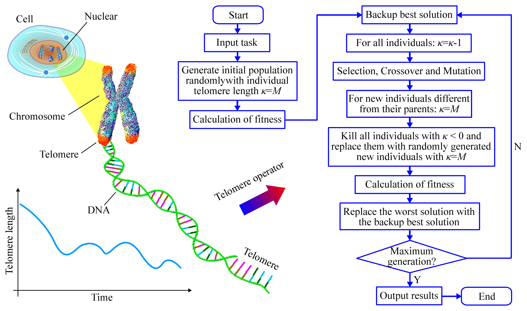
In applications, the performance of the telomere operator can be further improved by the following methods:
-
The initial length of the telomere is variable. If the fitness of the optimal individual in the current generation does not change compared with that in the previous generation, ; if M is less than zero, M=0. Note that because the condition for individual elimination is κ<0 (not κ=0), M=0 does not mean that all individuals are regenerated. This method assumes that the length of the telomere is affected by environmental stress. When evolution slows down, the algorithm strengthens individual extinction and regeneration caused by the telomere.
-
When the old individual is eliminated, a new individual is produced by it through non-uniform mutation (Chauhan et al., 2021; Ma, 2021). This method has a strong capability of global search in the early stage, and changes to local fine search in the later stage. The position of mutation s () of the old individual is randomly selected, and its element λs is updated using the following equation:
and
where Umax and Umin are the upper and lower limits of λs, respectively, and are independent and identically distributed random variables that obey a uniform distribution in the interval [0,1], and g and G are the current generation and total number of generations of the genetic algorithm, respectively.
Based on the above algorithm, we take Θxi=0.1, Θyi=0.1, and Θδi=5∘ () to optimize the solutions map shown in Fig. 9, and the result is shown in Fig. 11. It shows that the proportion of available solutions after optimization increases from 0.108579 to 0.871961.
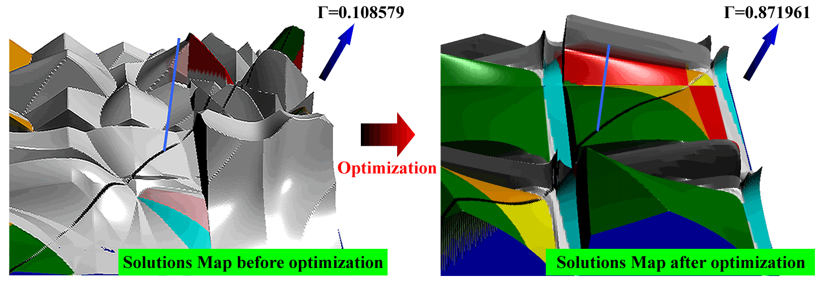
Figure 11Genetic algorithm-based optimization of solutions map based on the telomere operator.
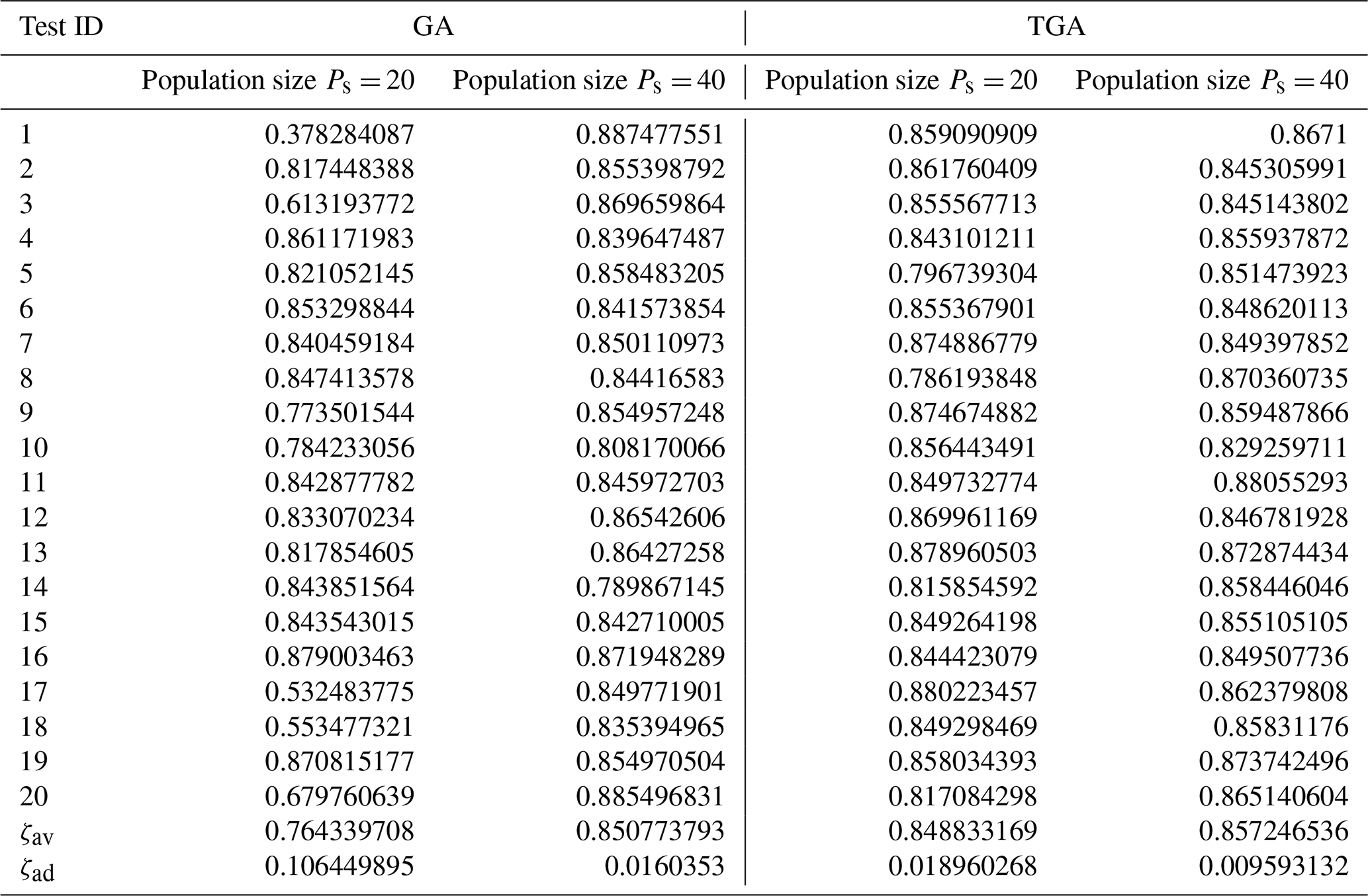
To further verify the effectiveness of the telomere operator, the results of optimization of the standard genetic algorithm (GA) and the telomere genetic algorithm (TGA) were compared with populations of Ps=20 and Ps=40, respectively, as shown in Table 7. Each group of optimization tests was repeated 20 times, and the parameters used in the calculation were as follows: total number of generations Gt=30, crossover probability Pc=0.6, mutation probability Pm=0.1, and initial telomere length M=3. In addition, float encoding, traditional roulette wheel selection, arithmetical crossover, a non-uniform mutation operator, and the elitist strategy were used by both the GA and the TGA during calculations. To compare their performance, the average ζav was used to measure the overall fitness values obtained by the algorithm while the average deviation ζad was used to express fluctuations in these values:
where yi is the best fitness of the algorithm in the ith test. Table 7 shows that when the population was 40, the performance of the TGA was equivalent to that of the GA. The average fitness and average deviation values of both were close. However, when the population was 20, the GA struggled to converge to the global optimal solution and there were large fluctuations in the data, while the TGA could still calculate normally. Its average fitness was 0.08449 higher than that of the GA and the average deviation in it was only 17.8 % of that in the GA. The telomere operator can thus avoid the premature convergence of the GA, especially when the population is small. This means that the TGA can use a small population to obtain approximately optimal results to save a significant amount of computing time.
Table 7Comparison of results of optimization of the GA and TGA.
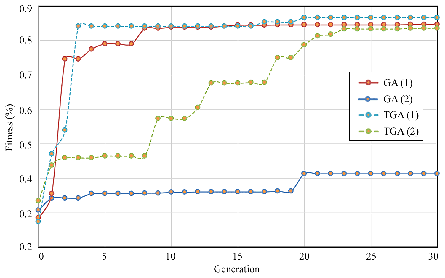
The typical fitness curves of the GA and TGA are shown in Fig. 12. Under normal circumstances, the optimal fitness value of the population rapidly improves in the initial stage of calculation of the genetic algorithm. Consider the curves of convergence “GA (1)” of the standard genetic algorithm and “TGA (1)” of the telomere genetic algorithm as examples: the initial fitness values of GA (1) and TGA (1) were below 0.2, but both increased to more than 0.7 within the first three generations. However, another form of the curve of convergence is also very common, where the GA prematurely falls into the local optimal solution. Consider the curves of convergence “GA (2)” of the GA and “TGA (2)” of the TGA as examples: when the GA falls into the local optimal solution, all individuals in the population are highly similar and the crossover operation can no longer produce a new solution. Although GA (1) jumped out of the local optimal solution through the mutation operation in the 20th generation, it fell into another local optimal solution and finally failed to achieve global convergence. By sharp contrast, TGA (2) could still generate new solutions with the help of the telomere operator after falling into the local optimal solution, jumping out of the local optimal solution many times until it achieved global convergence. We can glean important information from TGA (2): a large number of local optimal solutions may be distributed in the solution domain of optimization problems of the solutions map, where this is similar to the domain of solutions of multi-modal functions. Based on this assumption, we think that increasing the population size helps to expand the search scope of the algorithm. However, the telomere operator, which can enable the algorithm to jump repeatedly between local optimal solutions, can achieve a similar effect and is clearly more efficient.
5.3 Obtaining solutions maps with more options
In general, the GA can only obtain a solution with the highest fitness after convergence. However, a solutions map with a high fitness does not necessarily mean that a satisfactory solution can be obtained. In the problem of synthesis of linkage positions, the evaluation of the solution is multi-faceted. In addition to the absence of kinematic defects, the linkage solution needs to satisfy geometric constraints, such as the length of the linkage and position of installation, as well as the requirements of mechanical performances, such as kinematics and dynamics. Therefore, even if the proportion of available solutions of the optimized solutions map is very high, the solutions it provides may still be completely rejected in the subsequent analysis due to limitations imposed by other conditions of evaluation. A more feasible method is to generate multiple solutions maps to provide designers with more candidate solutions. If the optimal solutions map cannot provide a satisfactory solution, we can continue to search for feasible solutions in other solutions maps. Niche technology is used in this study to obtain multiple solutions maps through a single optimization. This can help to maintain the diversity of the population in the GA to prevent all individuals from converging to the same solution. Current niche technologies include the sharing function and the crowding mechanism (Che et al., 2021; Liu et al., 2020). This study uses the sharing function method. The sharing function Λ is used to measure the similarity between solutions:
where Π1 represents the genotypic distance between solution vectors Xi and Xj, Π2 represents the phenotypic distance between them, and μ1 and μ2 are the maximum individual distances of the genotype and the phenotype in the niche technology, respectively.
The modified fitness function Ψ* can then be expressed as:
when the value of the sharing function between an individual and all other individuals is large, its fitness is reduced to prevent the individual with the highest fitness from assimilating the entire population and maintain the diversity of the population. Therefore, niche technology can be used to obtain the optimal solution as well as a series of local optimal solutions that are different from one another.
In Eq. (27), the measurement of similarity by the sharing function depends on two distance functions, Π1 and Π2. Genotypic similarity between individuals is represented by Π1. For a real-coded solution vector, Π1 can be expressed by the Euclidean distance:
In this study, Π1 is not necessary because we attend more to the similarity of phenotypes than genotypes. By contrast, Π2 is important for representing (phenotypic) similarity. In the traditional sharing function method, Π2 is usually expressed by a fitness distance. However, the fitness function Ψ here represents the proportion of available solutions in the solutions map, and not the similarity between solutions maps. Therefore, a pseudo-histogram method for measuring the similarity between solutions maps is proposed. The histogram is used to describe the frequency distribution of different colors in an image. The solutions map has the characteristics of an image, and as a result, the histogram method can be used to describe the number distribution of eight kinds of linkages in the solutions map. However, the solutions map is not an image in the real sense. Hence, the corresponding histogram is called a “pseudo-histogram” in this study. If the pseudo-histogram is used as the feature of the solutions map, the similarity between any two maps can be measured by the Bhattacharyya coefficient:
where Ξ (X) represents the histogram vector corresponding to the solution vector X, which has eight elements. Each represents the number of solutions with a specific linkage type. The subscript i of Ξ indicates the index of the ith element in the histogram vector.
By embedding the sharing function based on the pseudo-histogram into the fitness function of the TGA, multiple groups of solutions maps can be obtained in a single calculation. Consider once again the position synthesis task in Table 4 as an example. Four groups of typical solutions maps obtained based on the above algorithm are shown in Fig. 13. It is clear that the Bhattacharyya coefficient calculated from the pseudo-histogram can adequately reflect the similarity between different solutions maps. Moreover, the niche realized by the pseudo-histogram can avoid the convergence of the GA to the same solution.
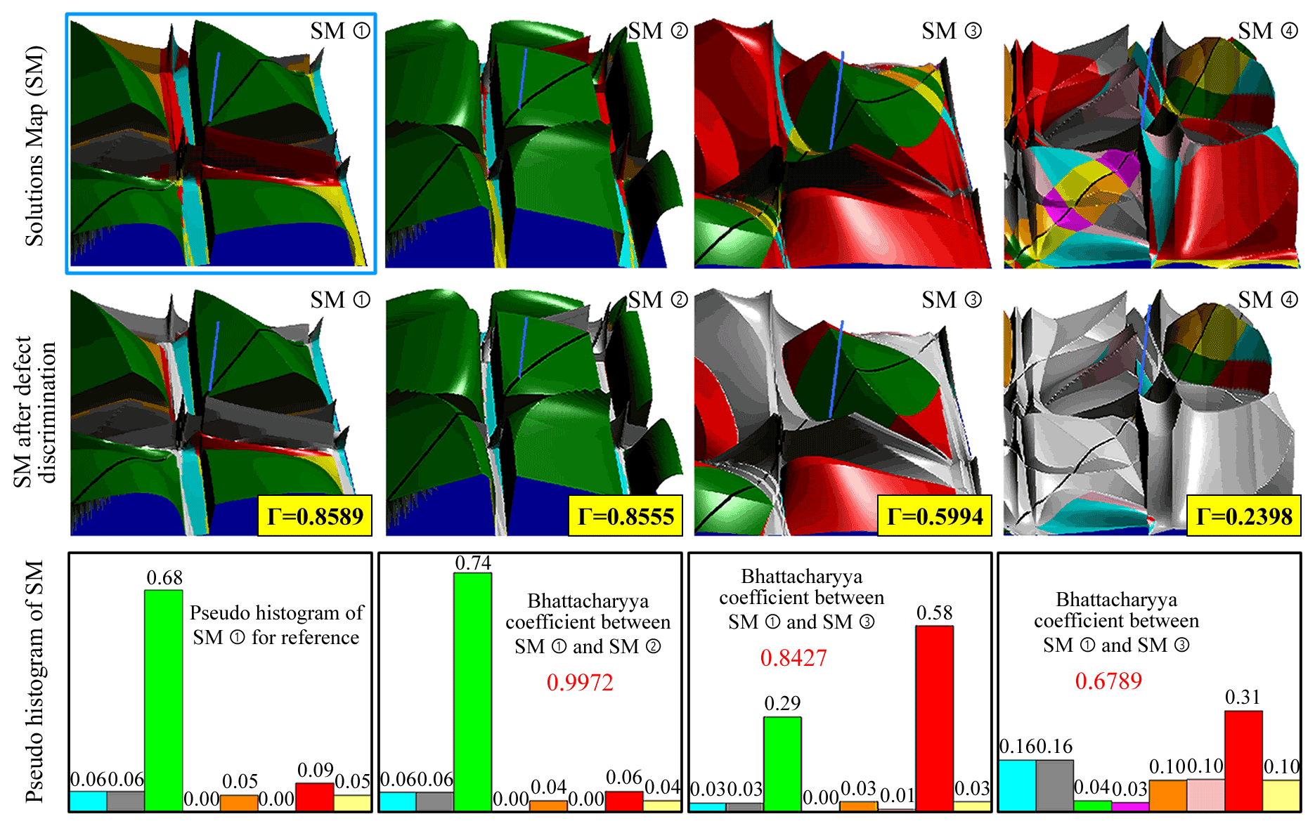
Figure 13Solutions maps generated by the niche genetic algorithm based on the pseudo-histogram method.
To further verify the influence of the niche technology based on the pseudo-histogram on the GA, the results of optimization of the GA and the TGA were compared with populations of Ps= 20 and Ps= 40, as shown in Table 8. It shows that the niche technology based on the sharing function method had a significant impact on the GA. The maximum fitness value obtained by optimization was generally low and unstable. Even if the population was expanded to 40, the fitness value obtained from three tests (ID = 2, 4, 9) was below 0.7 because the sharing function method changed the standard of fitness evaluation. The fitness of a solution depends not only on the objective function, but also on the similarity between it and the entire population. According to the previous assumptions, many local optimal solutions might have been distributed in the solution domain of optimization problems of the solutions map, and the use of the sharing function generally reduces the fitness of these solutions. Therefore, only when the algorithm converges to the real global optimal solution, can we obtain stable and high-quality results of optimization. The standard GA can usually converge only to local optimal solutions with different fitness values after each optimization, where the fitness values of these solutions are generally low and different. This causes the results of optimization to greatly fluctuate. Although the expansion of the population helps to expand the search scope of the algorithm, it is difficult to ensure that part of the randomly generated individuals in the initial population fall into the vicinity of the global optimal solution for further search. In this case, the algorithm is still trapped in widely distributed local optimal solutions with low fitness. By contrast, the telomere operator can enable the GA to jump between local optimal solutions and thus can always converge to the global optimal solution. This renders the algorithm stable. For these reasons, the telomere operator is insensitive to population size, and this indicates that the required solutions maps can still be obtained with a smaller population to reduce computation time.
Table 8Comparison of results of niche optimization of the GA and TGA.

5.4 BurLink software based on solutions map method
The solutions map is a computer-aided method of synthesis. To improve the efficiency of synthesis, the linkage synthesis software BurLink was developed based on the solutions map, as shown in Fig. 14. It offers two views. The right view is the solutions map and the left view shows the linkage solution selected from it. The movement of the buoy and the sea level in the solutions map can be controlled by sliders. When the buoy moves, the linkage solution and the coupler curve are updated immediately. The software can output the coordinates of each hinge on the linkage and show the corresponding animation.
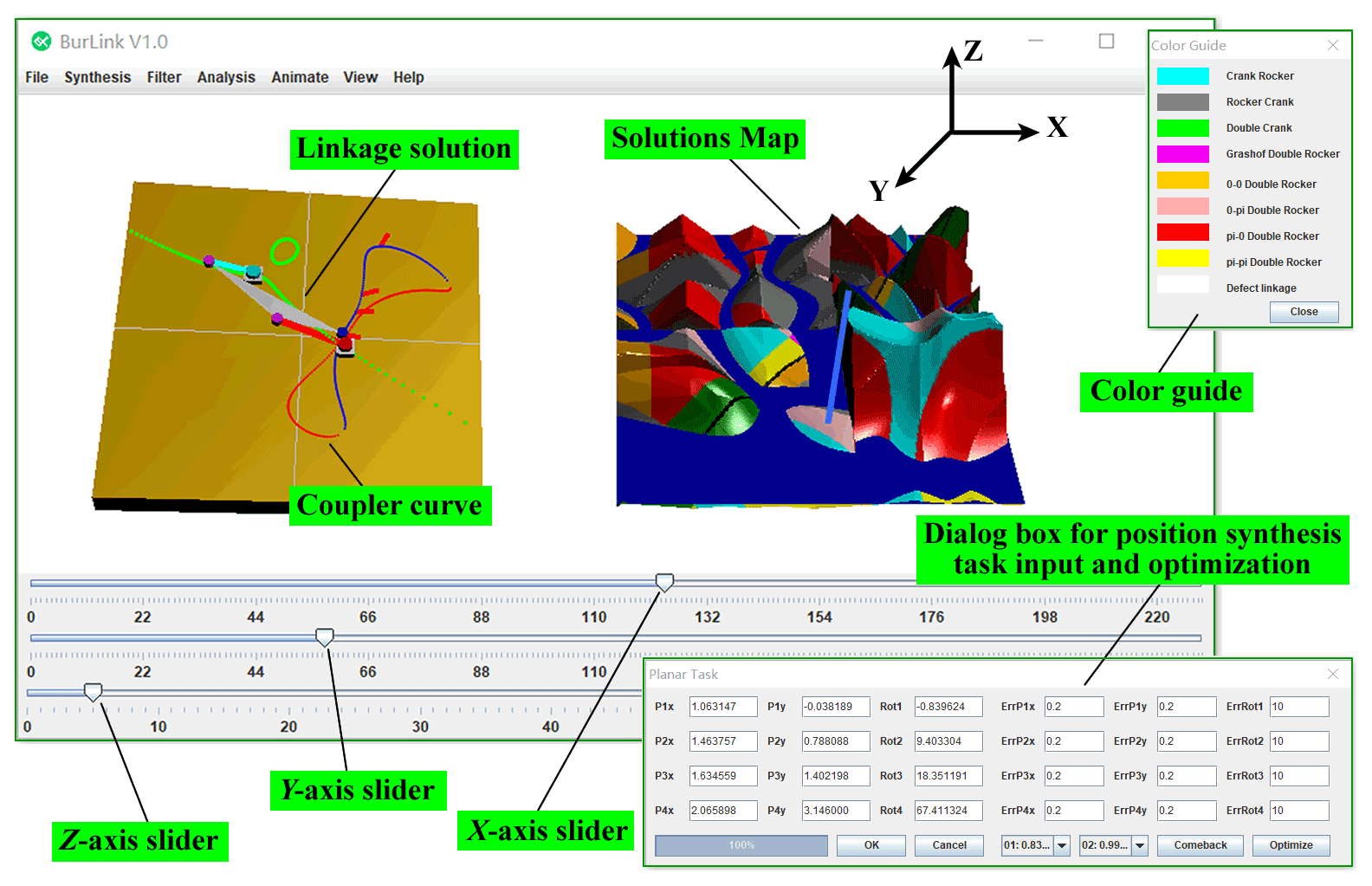
In addition to the calculation of points on the center and the circle, each linkage solution in the solutions map requires the calculation and visualization of the types of linkage and defect, and transmission-related performance. If the time needed for the calculation is too long, the synthesis efficiency of the software decreases. Most of the computation time is spent on the visualization of the solutions map. To shorten this, the Java3D API is used to generate the solutions map. Consider the solutions map shown in Fig. 5 as an example. BurLink can complete all calculations and the 3D display of 52 441 solutions within 300 ms (test conditions: 11th Gen Intel(R) Core(TM) i7-1165G7 at 2.80 GHz; RAM 16 GB). It also supports the TGA in expanding the domain of solution of the solutions map. After TGA optimization, users can extract information on any individual in the population and update the map.
5.5 Discussion
According to the analysis in Sect. 1, past methods can be divided into three categories: traditional method based on region-based segmentation technology, type map based on solution domain analysis, and approximate motion synthesis based on optimization. Both the type map and TGA-based solutions map can be used to analyze the solution domain; thus their synthesis efficiencies are much higher than that of the traditional, blind method. Compared with the type map, the TGA-based solutions map adds a dimension to visualize continuous attributes of the linkage, and can expand the solution domain through the TGA and niche technology. Although the TGA-based solutions map also uses the optimization algorithm, its objective of optimization is the solution domain and not a single linkage solution. In addition, it blurs the boundary between accurate position synthesis and approximate motion synthesis, which means that the two problems can be solved by a unified method in some cases. When the allowable errors in all guidance positions are zero, the TGA-based solutions map solves the problem of accurate position synthesis; when errors are introduced to part of the guidance positions, it solves the mixed problem of exact–approximate synthesis; when errors are introduced to all guidance positions, it solves the problem of approximate motion synthesis.
Compared with previous methods, the highlight of the proposed TGA-based solutions map is that it can provide more candidate solutions for the problem of the four-position synthesis of the 4R linkage to satisfy the needs of subsequent design. Consider the synthesis task in Table 4 as an example once again. Statistical results show that the number of candidate solutions that can be obtained by the type map or the basic solutions map is 5694, whereas the number of candidate solutions that can be obtained by the TGA-based solutions map is 25 670. Considering that solutions in the area of the same linkage type of the type map or the solutions map are highly similar, it is not rigorous enough to compare the two methods in terms of the number of candidate solutions only. If the linkage needs to be free of motion-related defects and the minimum transmission angle at the four specified positions is greater than 30∘, the region in the solution domain that satisfies the above constraints and has the same linkage type can be called the candidate region. As is shown in Fig. 15, the type map can provide 9 candidate regions for the synthesis task in Table 6 while the solutions map based on the TGA and niche technology (population size, Ps= 20) can provide 20 solution domains and a total of 208 candidate regions. In particular, the solutions map can find solutions of all linkage types, but the type map cannot find the rocker crank and Grashof double-rocker linkage solutions that satisfy the given requirements. Note that only the transmission angle is limited here. If the ratio of the link length, velocity and acceleration of the guidance point, force of the driving link, and other attributes are limited, the nine candidate regions provided by the type map are likely to be significantly reduced or may even lead to no solution. By contrast, after the expansion of the solution domain, the solutions map still has a larger selection space owing to the large number of regions of candidate solutions.

Figure 15Analysis of candidate regions. (a) Schematic diagram of candidate regions in the solutions map. (b) Number of candidate regions with different types of linkages.
In this paper, the authors examined the computer-aided synthesis of the planar 4R linkage. The main conclusions can be summarized as follows:
-
A solutions map method was proposed. It can reveal the distribution of the linkage solutions of different attributes, including discontinuous attributes (such as linkage and defect types) and continuous attributes (such as link length, transmission angle, acceleration, and force, or their weighted values) so that the required linkage solutions can be quickly located.
-
A method of generating the solutions map was proposed. The center curve was first calculated by projective geometry and the circle curve was then obtained by vector elimination. A defect discrimination algorithm was proposed based on this which can quickly eliminate defective linkage solutions from the solutions map to improve the efficiency of linkage synthesis.
-
An improved genetic algorithm (GA) based on the telomere operator was proposed and used to expand the domain of solution of the solutions map. A niche construction method based on a pseudo-histogram was proposed based on this, such that more solutions maps and candidate solutions can be obtained after optimization. The results showed that the telomere genetic algorithm (TGA) significantly outperformed the traditional GA regarding the problem of expanding the domain of solutions of the solutions map.
-
The TGA-based solutions map was used to develop the software BurLink for linkage synthesis.
-
Compared with previous research, the proposed TGA-based solutions map can provide more candidate solutions for the problem of the four-position synthesis of the 4R linkage. Moreover, it blurs the boundary between accurate position synthesis and approximate motion synthesis, which means that the two problems can be solved by a unified method in some cases.
-
The TGA-based solutions map can also be applied to the finite positional synthesis of any linkage with at least two free variables, including planar and spatial linkages. The specific method of operation is consistent with that in this study. It is first necessary to specify two free variables in the linkage synthesis model to form the solutions map and to then use the TGA to optimize it.
All the data used in this paper can be obtained by request from the corresponding author.
YZ, LX, and GW wrote the paper and participated in the algorithm discussion of constructing the telomere genetic algorithm (TGA). YZ wrote the fast validation program of TGA under MATLAB. GW proposed the concept of TGA and solutions map, developed BurLink software and transplanted YZ's TGA program from MATLAB to BurLink. LX provided all the test data required for the paper based on BurLink. FZ, YS, and HZ edited and verified all the formulas and pictures used in this paper.
The contact author has declared that none of the authors has any competing interests.
Publisher's note: Copernicus Publications remains neutral with regard to jurisdictional claims in published maps and institutional affiliations.
This research has been supported by the Shandong Provincial Natural Science Foundation (grant no. ZR2020QE163), the Program of Shandong Provincial Key Laboratory of Horticultural Machineries and Equipment (grant no. YYJX-2019-01), the Shandong Provincial Key Research and Development Program (grant no. 2018GNC112008) and the China Agriculture Research System of MOF and MARA (grant no. CARS-27).
This research has been supported by the Shandong Provincial Natural Science Foundation (grant no. ZR2020QE163), the Program of Shandong Provincial Key Laboratory of Horticultural Machineries and Equipment (grant no. YYJX-2019-01), the Shandong Provincial Key Research and Development Program (grant no. 2018GNC112008), and the China Agriculture Research System of MOF and MARA (grant no. CARS-27).
This paper was edited by Francisco Romero and reviewed by two anonymous referees.
Baskar, A. and Bandyopadhyay, S.: A homotopy-based method for the synthesis of defect-free mechanisms satisfying secondary design considerations, Mech. Mach. Theory, 133, 395–416, https://doi.org/10.1016/j.mechmachtheory.2018.12.002, 2019.
Cao, Y. and Han, J.: Solution region-based synthesis methodology for spatial HCCC linkages, Mech. Mach. Theory, 143, 103619, https://doi.org/10.1016/j.mechmachtheory.2019.103619, 2020.
Cera, M. and Pennestrì, E.: Generalized Burmester points computation by means of Bottema's instantaneous invariants and intrinsic geometry, Mech. Mach. Theory, 129, 316–335, https://doi.org/10.1016/j.mechmachtheory.2018.07.011, 2018.
Cera, M. and Pennestrì, E.: The mechanical generation of planar curves by means of point trajectories, line and circle envelopes: A unified treatment of the classic and generalized Burmester problem, Mech. Mach. Theory, 142, 103580, https://doi.org/10.1016/j.mechmachtheory.2019.103580, 2019.
Chauhan, S., Singh, M., and Aggarwal, A. K.: Diversity driven multi-parent evolutionary algorithm with adaptive non-uniform mutation, J. Exp. Theor. Artif. In., 33, 775–806, https://doi.org/10.1080/0952813X.2020.1785020, 2021.
Che, Z. H., Chiang, T. A., and Lin, T. T.: A multi-objective genetic algorithm for assembly planning and supplier selection with capacity constraints, Appl. Soft Comput., 101, 107030, https://doi.org/10.1016/j.asoc.2020.107030, 2021.
Erdman, A. G. and Loftness, P. E.: Synthesis of linkages for cataract surgery: storage, folding, and delivery of replacement intraocular lenses (IOLs), Mech. Mach. Theory, 40, 337–351, https://doi.org/10.1016/j.mechmachtheory.2004.07.006, 2005.
Filemon, E.: Useful ranges of centerpoint curves for design of crank-and-rocker linkages, Mech. Mach. Theory, 7, 47–53, https://doi.org/10.1016/0094-114X(72)90015-8, 1972.
Ge, Q. J., Purwar, A., Zhao, P., and Deshpande, S.: A Task-driven approach to unified synthesis of planar four-bar linkages using algebraic fitting of a pencil of G-manifolds, J. Comput. Inf. Sci. Eng., 17, 031011, https://doi.org/10.1115/1.4035528, 2017.
Gogate, G. R. and Matekar, S. B.: Optimum synthesis of motion generating four-bar mechanisms using alternate error functions, Mech. Mach. Theory, 54, 41–61, https://doi.org/10.1016/j.mechmachtheory.2012.03.007, 2012.
Gogate, G. R. and Matekar, S. B.: Unified synthesis of Watt-I six-link mechanisms using evolutionary optimization, J. Mech. Sci. Technol., 28, 3075–3086, https://doi.org/10.1007/s12206-014-0715-0, 2014.
Gupta, K. C. and Beloiu, A. S.: Branch and circuit defect elimination in spherical four-bar linkages, Mech. Mach. Theory, 33, 491–504, https://doi.org/10.1016/S0094-114X(97)00078-5, 1998.
Han, J. and Cao, Y.: Solution Region Synthesis Methodology of RCCC Linkages for Four Poses, Mech. Sci., 9, 297–305, https://doi.org/10.5194/ms-9-297-2018, 2018.
Jia, G., Huang, H., Wang, S., and Li, B.: Type synthesis of plane-symmetric deployable grasping parallel mechanisms using constraint force parallelogram law, Mech. Mach. Theory, 161, 104330, https://doi.org/10.1016/j.mechmachtheory.2021.104330, 2021.
Jin, Z. and Shi, Y.: Computer drafting of center curve, Journal of North China University of Technology, 3, 76–85, 1991.
Liang, C. and Chen, H.: Calculation and Design of Planar Linkage, Higher Education Press, Beijing, China, ISBN: 7-04-003936-2, 1993.
Liu, H. and Han, J.: Solution region synthesis methodology of spatial 1CS-4SS linkages for six given positions, Mech. Mach. Theory, 162, 104369, https://doi.org/10.1016/j.mechmachtheory.2021.104369, 2021.
Liu, J., Liu, J., Yan, X., and Peng, B.: A heuristic algorithm combining Pareto optimization and niche technology for multi-objective unequal area facility layout problem, Eng. Appl. Artif. Intel., 89, 103453, https://doi.org/10.1016/j.engappai.2019.103453, 2020.
Martin, D. T. and Murray, A. P.: Developing classifications for synthesizing, refining, and animating planar mechanisms, in: ASME 2002 International Design Engineering Technical Conferences and Computers and Information in Engineering Conference, 29 September–2 October 2002, Montreal, Quebec, Canada, 1397–1403, https://doi.org/10.1115/DETC2002/MECH-34372, 2002.
Ma, Z., Li, S., Wang, Y., and Yang, Z.: Component-level construction schedule optimization for hybrid concrete structures, Automat. Const., 125, 103607, https://doi.org/10.1016/j.autcon.2021.103607, 2021.
McCarthy, J. M.: Kinematic Synthesis, in: 21st Century Kinematics, edited by: Antman, S. S., Marsden, J. E., and Sirovich, L., Springer, London, e-ISBN: 978-1-4419-7892-9, ISBN: 978-1-4419-7891-2, https://doi.org/10.1007/978-1-4419-7892-9, 2013.
Nachaoui, M., Afraites, L., and Laghrib, A.: A regularization by denoising super-resolution method based on genetic algorithms, Signal Process.-Image, 99, 116505, https://doi.org/10.1016/j.image.2021.116505, 2021.
Oliveira, B. B., Carravilla, M. A., and Oliveira, J. F.: A diversity-based genetic algorithm for scenario generation, Eur. J. Oper. Res., 299, 1128–1141, https://doi.org/10.1016/j.ejor.2021.09.047, 2022.
Ravani, B. and Roth, B.: Motion Synthesis using kinematic mappings, ASME J. Mech. Trans. and Automation, 105, 460–467, https://doi.org/10.1115/1.3267382, 1983.
Ruth, D. A. and McCarthy, J. M.: The design of spherical 4R linkages for four specified orientations, Mech. Mach. Theory, 34, 677–692, https://doi.org/10.1016/S0094-114X(98)00048-2, 1999.
Shirazi, K. H.: Computer modelling and geometric construction for four-point synthesis of 4R spherical linkages, Appl. Math. Model., 31, 1874–1888, https://doi.org/10.1016/j.apm.2006.06.013, 2007.
Singh, R., Chaudhary, H., and Singh, A. K.: Defect-free optimal synthesis of crank-rocker linkage using nature-inspired optimization algorithms, Mech. Mach. Theory, 116, 105–122, https://doi.org/10.1016/j.mechmachtheory.2017.05.018, 2017.
Sundram, S. and Larochelle, P.: Using optimization for the mixed exact-approximate synthesis of planar mechanisms, in: ASME 2015 International Design Engineering Technical Conferences and Computers and Information in Engineering Conference, 2–5 August 2015, Boston, Massachusetts, USA, V05BT08A081, https://doi.org/10.1115/DETC2015-47394, 2015.
Sun, J. W. H. and Waldron, K. J.: Graphical transmission angle control in planar linkage synthesis, Mech. Mach. Theory, 16, 385–397, https://doi.org/10.1016/0094-114X(81)90012-4, 1981.
Tipparthi, H. and Larochelle, P.: Orientation order analysis of spherical four-bar mechanisms, J. Mech. Robot., 3, 044501, https://doi.org/10.1115/1.4004898, 2011.
Trejo, O. M., Villar, C. A. C., Escalante, R. P., Arjona, M. A. Z., and Peñuñuri, F.: Synthesis method for the spherical 4R mechanism with minimum center of mass acceleration, Mech. Mach. Theory, 93, 53–64, https://doi.org/10.1016/j.mechmachtheory.2015.04.015, 2015.
Waldron, K. J. and Strong, R. T.: Improved solutions of the branch and order problems of burmester linkage synthesis, Mech. Mach. Theory, 13, 199–207, https://doi.org/10.1016/0094-114X(78)90043-5, 1978.
Wilhelm, S. R., Sullivan, T., and Ven, J. D. V.: Solution rectification of slider-crank mechanisms with transmission angle control, Mech. Mach. Theory, 107, 37–45, https://doi.org/10.1016/j.mechmachtheory.2016.09.011, 2017.
Zhang, S.: Design of Planar Linkage, Higher Education Press, Beijing, China, China Book Number 150100509, 1983.
Zhao, Y.: Analysis and Synthesis of Agricultural Machinery, China Machine Press, Beijing, China, ISBN: 978-7-111-25000-5, 2009.