Synthesis of trigonometric motion programs with lower motion characteristics

Motion characteristics are dimensionless peak values of velocity, acceleration, jerk, and acceleration multiplied by velocity of a motion program. In general, these peak values of synthesized motion programs should be as low as possible. Some trigonometric motion programs are widely used because they have a good compromise of all motion characteristics. A property in common for trigonometric motion programs is that their acceleration functions can be expressed as a qualitative shape of a sinusoidal function. The interval of the sinusoidal function is divided into several zones having different linear slopes. The acceleration function can be easily shaped by specifying presented phase angle function to synthesize desired motion programs. To improve the kinematic quantities of trigonometric motion programs, this paper addresses an alternative phase angle function to obtain synthesized motion programs with simultaneous reduction in all the motion characteristics. The synthesis process and results are illustrated by examples.

1 Introduction

A cam mechanism is a simple but effective way of transforming an ordinary motion into an intricate output motion. Because a cam mechanism can meet a wide variety of desired motion requirement, it has been implemented in many different designs and has a wide range of applications (Neklutin, 1969; Chen, 1982; Jensen, 1987; Reeve, 1995; Rothbart, 2003; Norton, 2009). In order to make the cam mechanism perform better, its camshaft will usually be designed to operate as fast as possible, such that a follower can finish a desired motion in a shorter time. However, the angular velocity of a camshaft cannot be infinitely increased because stored kinetic energy, inertia force, and the vibration of a follower are critical restrictions against the angular velocity of the camshaft. These kinematic responses of cam mechanisms are directly correlated to the velocity, acceleration, and jerk function of its follower. If peak values of the velocity, acceleration, and jerk function of the follower are smaller, then the kinetic energy, inertia force, and vibration imposed on the follower will correspondingly lighter. Consequently, apart from meeting the predetermined design requirements, it is also important to synthesize a motion program with lower peak values of velocity, acceleration, and jerk, especially for high-speed cams.

Over the years, many investigations had been reported for the synthesis of motion programs. Both Zigo (1967) and Chen (1969, 1972) introduce a numerical algorithm in the construction of a motion program with an arbitrary form of acceleration function. Angeles (1983) address an approximation of a dwell-rise-dwell motion program using a periodic spline to meet the curve continuity up to acceleration. Lakshminarayana and Kumar (1987) suggest using a finite trigonometric series to avoid a high frequency if it is unnecessary for the dwell motion to be exact. Tsay and Huey (1988, 1989) propose using spline functions to synthesize the cam motion program and analyze the dynamic behavior of a cam with a non-rigid follower. Sandgren and West (1989) describe and optimize a follower acceleration curve by a B-spline representation. They later extend the flexibility of spline function by introducing rational B splines (Tsay and Huey, 1993) to synthesize the motion program. Yoon and Rao (1993) apply minimum norm principle to minimize the peak values of acceleration and jerk of a synthesized cam motion program using cubic splines. The Bézier technique for motion program synthesis is addressed by Ting et al. (1994). Their method offers an institutive way to control boundary conditions by adding basic and auxiliary control points. Yan et al. (1996a, b) consider reducing the peak values of the follower's kinematics by varying the cam input angular velocity both theoretically and experimentally. Wang and Yang (1996) synthesize the displacement function by the piecewise polynomial of the spline function. Their approach allows a direct control of the shape of synthesized curves by imposing the continuity conditions on the breaking points of curves. Neamtu et al. (1998) demonstrate how to design the displacement function of the follower based on the use of trigonometric splines. Srinivasan and Ge (1998) replace traditional polynomial curves with Bernstein–Bézier harmonic curves to represent the cam displacement functions with low-harmonic content. Cheng (2002) provides a generalized acceleration modal for synthesizing motion curves efficiently by specifying the shape function and design parameters. A cubic spline with more than eight knots (Kim et al., 2002) is chosen to optimize the motion of a variable speed cam. Lampinen (2003) represents the displacement function of the follower by a sixth degree B spline. In doing so, the motion program can be expressed in a parametric form and optimized effectively by the genetic algorithm. Mermelstein and Acar (2004) explain the limitation of the piecewise polynomial (Wang and Yang, 1996) and then refine it. They turn boundary and continuity satisfactions into a set of linear equations, which can be more easily implemented in optimization process. Qiu et al. (2005) apply a uniform B spline to synthesize motion program and optimize their design by an improved complex search algorithm. The weighted coefficient values of optimization can automatically be adjusted using their method. Nguyen and Kim (2007) illustrate how to ensure kinematic continuity up to the acceleration function by using a cubic spline. Furthermore, they also demonstrate how to obtain a continuous jerk function by using a quantic spline curve. A fractional polynomial function (Acharyya and Naskar, 2008) is introduced to yield a modified trapezoid curve with lower acceleration and jerk functions. Mandal and Naskar (2009) discuss the effect of introducing a control point in a B-spline synthesis of the cam motion program and verify their theoretical prediction experimentally (Naskar and Mandal, 2012). Sateesh et al. (2009) focus on the design of velocity function represented by a 3rd degree B-spline polynomial with six control points. Flocker (2012) presents a modified trapezoidal acceleration profile whose magnitude can be adjusted freely based on designer's choice. Flocker and Bravo (2012) consider a specific motion program which has a constant velocity segment that aims towards minimizing the cycle times. Cardona et al. (2013) and Hidalgo-Martinez et al. (2014) further apply Bézier curves to ensure kinematic performances of synthesized cam mechanisms. To improve the transient and heavy load capacity of cam mechanisms, Yang et al. (2014) propose a composite cam motion program which combines an involute with a quadratic curve. Sateesh (2014) aims to reduce the velocity, acceleration, and jerk peak values by using non-uniform rational B spline (NURBS) to describe cam motion programs. Zhou et al. (2016) address how to reduce the vibration and impact velocity of cam mechanisms by applying a Fourier series to the displacement function synthesis. To improve motion features of cycloidal motion, a 5th order B spline with eight control points (Sahu et al., 2016) is used to approximate the cycloidal curve with high velocity, uniform acceleration, and minimum jerk. Nguyen et al. (2019) formulate a general follower motion synthesis method using NURBS function. Their method can satisfy arbitrary boundary conditions. Meanwhile, by manipulating the knot vector and the weight factor of the NURBS function, the peak values of the acceleration and jerk function can be minimized. To eliminate higher order discontinuity and extreme peak values of the cam motion program, Yu et al. (2019) use a Bernstein–Lagrange basis function as an interpolation method to fulfill the multi-order derivatives. In addition, they also develop a shape adjustment method to lower the peak values of cam motion programs. It can be observed that, while a great amount of efforts had been put in the synthesis of cam motion programs using spline functions, trigonometric motion programs are still not a fully developed domain and could be a potentially innovative area worthy of investigation. In addition, although diversified approaches have been addressed by many researchers, the main theme of cam motion synthesis always relates to ensuring the continuity and reducing the maximums of motion kinematics.

In a synthesizing cam motion program, velocity, acceleration, and jerk functions are the main characteristics under investigation. Among these kinematic characteristics, the acceleration function is the most influential factor because the physical nature of the cam–follower mechanism is mainly modeled by the acceleration function. The acceleration of a follower increases the inertia forces contributing to the loading of cam mechanisms. The inertia load is proportional to the acceleration function of a follower. If the acceleration of the follower is too large, higher than normal force will be induced, and contact forces usually result in undesired wear at the cam–follower contact interface. For force-closed cam mechanisms, the inertial forces of the followers must be counteracted by spring forces to keep the contact between the cam and follower. If the negative acceleration of the follower is too large, a higher spring force is needed to ensure that the negative inertia load does not exceed the available spring force. In doing so, an increased spring force will increase the additional load to the system, which may be an unwise solution. It can be concluded that the acceleration of the follower is an important factor, and its peak value should be designed to be as low as possible.

Apart from the peak value of the acceleration function worth considering, the location where the maximum acceleration occurs is another critical issue worthy of investigation. The peak value of the synthesized acceleration function should be in the early and late rising motion (Volmer, 1972). The early accelerating peak causes a high inertia force to counteract with lower spring force. Thus, a lower contact force will be induced at the cam–follower contact. The late decelerating peak allows the spring to nearly reach its maximum compression and provide enough contact force to prevent the follower jump (Volmer, 1972). In other words, there only needs a spring with lower stiffness, which also leads to an overall reduction in the contact forces. As suggested, both the magnitude and location of the maximum acceleration are important for the synthesis of the cam motion program.

In summary, few studies have been done on the synthesis of trigonometric motion programs. To fill this void, we confine the discussion to trigonometric motion programs. In addition, we propose adequately shaping the acceleration function ahead of either velocity or jerk functions because the acceleration function greatly affects the physical nature of the cam–follower mechanism. One of the contributions of this paper is the characterization of a family of trigonometric motion programs by a simplified and uniform function. The proposed function is in the form of a sinusoidal function, which is used to describe the acceleration function of a family of trigonometric motion programs. To generalize the acceleration of trigonometric motion programs by a sinusoidal function, the interval of the sinusoidal function is divided into several zones. The acceleration function can be easily shaped by specifying zone arrangements to obtain desired the motion programs. This paper also proposes alternative design equations for synthesizing trigonometric motions with lower peak values of kinematic quantities. For a direct comparison, synthesized motions programs are compared with the conventionally used motions, such as cycloidal motion (CYC), modified sinusoidal motion (MS), modified trapezoidal motion (MT), and modified constant velocity 50 motion (MCV50). Results indicate that employing the presented design equations for motion synthesis does lead to a simultaneous reduction in peak values of velocity, acceleration, jerk, and acceleration multiplied by velocity.

2 Motion program and its characteristic values

Motion programs are commonly used to specify an output motion of a follower in terms of certain input parameters. Specifically speaking, the output motion of a follower is characterized by its displacement S, velocity V, acceleration A, and jerk J functions. These curves can be a function of either time t or cam rotation angle θ. In synthesizing motion programs, if the cam is assumed to rotate at a constant angular velocity of 1 rad s⁻¹, then the synthesis process can be simplified. In doing so, motion programs are directly associated with the cam rotation angle (Neklutin, 1969). In addition, conventional displacement functions are mostly anti-symmetrical about their inflection point $(\mathit{\theta },S)=(\mathit{\beta }/\mathrm{2},h/\mathrm{2})$ and satisfy the following:

$$\begin{array}{}\text{(1)}& S\left(\mathit{\beta }-\mathit{\theta }\right)=h-S\left(\mathit{\theta }\right),\end{array}$$

where S(θ) is the displacement function of a follower, β is the total period, and h is the total stroke. For such an anti-symmetrical function, its entire motion program can be fully determined once the first half portion of its motion program is specified. That is, motion programs for $\mathit{\beta }/\mathrm{2}\le \mathit{\theta }\le \mathit{\beta }$ can be determined once the motion programs $\mathrm{0}\le \mathit{\theta }\le \mathit{\beta }/\mathrm{2}$ have been derived (Volmer, 1972). In order to simplify the following discussion on the proposed modal, the motion programs are only considered on the interval $[\mathrm{0},\mathit{\beta }/\mathrm{2}]$.

Table 1 Characteristic values of conventional motion programs.

Figure 1 Normalized V, A, J, and A×V functions.

In general, for a specified follower motion with fixed lift h in the cam angle of β, peak values of synthesized velocity, acceleration, and jerk functions should be as low as possible. This criterion can be used to assess the synthesized motion programs. To fairly compare the peak values of synthesized motion programs, it is suggested that these functions be normalized and their normalized peak values compared. These normalized peak values are called motion characteristics (Neklutin, 1969; Jensen, 1987) of synthesized motion programs, including the velocity characteristic C_V, acceleration characteristic C_A, and jerk characteristic C_J. These coefficients can be expressed as follows:

$$\begin{array}{}\text{(2)}& {\displaystyle }{C}_{\mathrm{V}}=V_{max}\times {\displaystyle \frac{\mathit{\beta }}{h}}\text{(3)}& {\displaystyle }{C}_{\mathrm{A}}=A_{max}\times {\displaystyle \frac{{\mathit{\beta }}^{\mathrm{2}}}{h}}\text{(4)}& {\displaystyle }{C}_{\mathrm{J}}=J_{max}\times {\displaystyle \frac{{\mathit{\beta }}^{\mathrm{3}}}{h}}.\end{array}$$

The input torque is also an important factor worthy of investigation since it governs the size of the motor drive, the drive shaft, and related parts for handling the transfer of energy throughout the cam mechanism. To evaluate the factors affecting the input torque, it can be assumed that the infinitesimal work dW done by the follower of the mass m is expressed as follows:

$$\begin{array}{}\text{(5)}& \mathrm{d}W=m\times A\times \mathrm{d}S\left(\mathit{\theta }\right),\end{array}$$

where $A=\frac{{\mathrm{d}}^{\mathrm{2}}S\left(\mathit{\theta }\right)}{\mathrm{d}{\mathit{\theta }}^{\mathrm{2}}}{\mathit{\omega }}^{\mathrm{2}}$ is the acceleration of the follower, ω is the angular velocity of the camshaft, and dS(θ) is the infinitesimal displacement of the follower. In addition, the infinitesimal work dW is also equal to the input torque T multiplied by the infinitesimal displacement of the cam rotation angle dθ, namely, as follows:

$$\begin{array}{}\text{(6)}& \mathrm{d}W=T\times \mathrm{d}\mathit{\theta }.\end{array}$$

Therefore, from Eqs. (5) and (6), the input torque T can be rewritten as follows:

$$\begin{array}{}\text{(7)}& T=m{\mathit{\omega }}^{\mathrm{2}}{\displaystyle \frac{\mathrm{d}S}{\mathrm{d}\mathit{\theta }}}{\displaystyle \frac{{\mathrm{d}}^{\mathrm{2}}S\left(\mathit{\theta }\right)}{\mathrm{d}{\mathit{\theta }}^{\mathrm{2}}}},\end{array}$$

where $\frac{\mathrm{d}S}{\mathrm{d}\mathit{\theta }}$ and $\frac{{\mathrm{d}}^{\mathrm{2}}S\left(\mathit{\theta }\right)}{\mathrm{d}{\mathit{\theta }}^{\mathrm{2}}}$ are the velocity V(θ) function and the acceleration function A(θ) of the follower, respectively. Because mω² in Eq. (7) is constant, it can be found that the input torque is directly correlated with $\frac{{\mathrm{d}}^{\mathrm{2}}S\left(\mathit{\theta }\right)}{\mathrm{d}{\mathit{\theta }}^{\mathrm{2}}}\frac{\mathrm{d}S}{\mathrm{d}\mathit{\theta }}=A\left(\mathit{\theta }\right)\times V\left(\mathit{\theta }\right)$, which is the acceleration function multiplied by the velocity function of the follower. By normalizing the variables in the equations, the velocity and acceleration functions can be written as follows:

$$\begin{array}{}\text{(8)}& {\displaystyle }V\left(\mathit{\theta }\right)=v\left(\mathit{\theta }\right){\displaystyle \frac{h}{\mathit{\beta }}}\text{(9)}& {\displaystyle }A\left(\mathit{\theta }\right)=a\left(\mathit{\theta }\right){\displaystyle \frac{h}{{\mathit{\beta }}^{\mathrm{2}}}},\end{array}$$

where v(θ) and a(θ) are the normalized velocity and acceleration functions, respectively. Thus, the input torque T in Eq. (7) can be expressed as follows:

$$\begin{array}{}\text{(10)}& T=m{\mathit{\omega }}^{\mathrm{2}}{\displaystyle \frac{h^{\mathrm{2}}}{{\mathit{\beta }}^{\mathrm{3}}}}v\left(\mathit{\theta }\right)a\left(\mathit{\theta }\right).\end{array}$$

The maximum of the input torque T occurs when A(θ)×V(θ) reaches the maximum. Therefore, the torque characteristic C_M can be expressed as follows:

$$\begin{array}{}\text{(11)}& C_{\mathrm{M}}=(A\times V{)}_{max}\times {\displaystyle \frac{{\mathit{\beta }}^{\mathrm{3}}}{h^{\mathrm{2}}.}}\end{array}$$

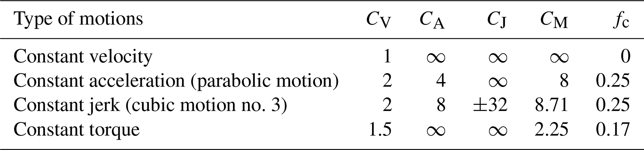
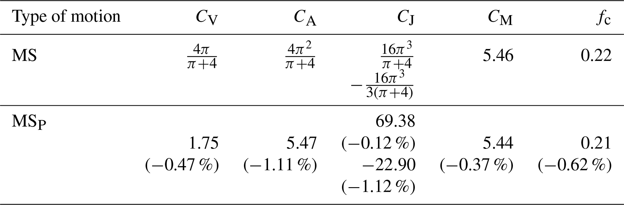
Table 1 shows characteristic values of conventional motion programs. Notice that the constant velocity motion has the lowest C_V of 1, the constant acceleration motion has the lowest C_A of 4, the constant jerk (cubic motion no. 3) motion has the lowest C_J of 32, and the constant torque motion has the lowest C_M of 2.25. The uniqueness of the constant torque motion lies in the multiplication of its velocity and acceleration. For a motion program to have the lowest torque characteristic, the multiplication of its velocity and acceleration function has to be a constant value. To derive the constant torque motion program, its analytical expression can be expressed as follows:

$$\begin{array}{}\text{(12)}& V\left(\mathit{\theta }\right)\times A\left(\mathit{\theta }\right)=C,\end{array}$$

where C is a constant coefficient. Rearranging Eq. (12) yields the following:

$$\begin{array}{}\text{(13)}& V\left(\mathit{\theta }\right)\times \mathrm{d}V\left(\mathit{\theta }\right)=C\mathrm{d}\mathit{\theta }.\end{array}$$

Integrating Eq. (13) and substituting a boundary condition V(θ)=0 when θ=0^∘ yields the following:

$$\begin{array}{}\text{(14)}& V\left(\mathit{\theta }\right)=\sqrt{\mathrm{2}C\mathit{\theta }}.\end{array}$$

Next, integrate Eq. (14) with respect to θ and substitute a boundary condition S(θ)=0 when θ=0^∘ to obtain the displacement equation of the constant torque motion program, namely, the following:

$$\begin{array}{}\text{(15)}& S\left(\mathit{\theta }\right)={\displaystyle \frac{\mathrm{2}\sqrt{\mathrm{2}C}{\mathit{\theta }}^{\frac{\mathrm{3}}{\mathrm{2}}}}{\mathrm{3}}}.\end{array}$$

Since the constant torque motion program is assumed as an anti-symmetrical function, we can substitute a boundary condition $S\left(\mathit{\theta }\right)=h/\mathrm{2}$ when $\mathit{\theta }=\mathit{\beta }/\mathrm{2}$ to yield the following:

$$\begin{array}{}\text{(16)}& C=\mathrm{2.25}{\displaystyle \frac{h^{\mathrm{2}}}{{\mathit{\beta }}^{\mathrm{3}}}}.\end{array}$$

Therefore, Eq. (15) can be rewritten as follows:

$$\begin{array}{}\text{(17)}& S\left(\mathit{\theta }\right)=\sqrt{\mathrm{2}}h{\left({\displaystyle \frac{h}{\mathit{\beta }}}\right)}^{\mathrm{1.5}}.\end{array}$$

One may further notice that each motion only has one kind of motion characteristic, which is the lowest bound. However, the rest of its motion characteristics are either infinite or considerably large. This means that a motion program that suits any kind of kinematic problems does not exist. Hence, a general rule for synthesizing a motion program is to have its C_V, C_A, C_J, and C_M simultaneously as low as possible.

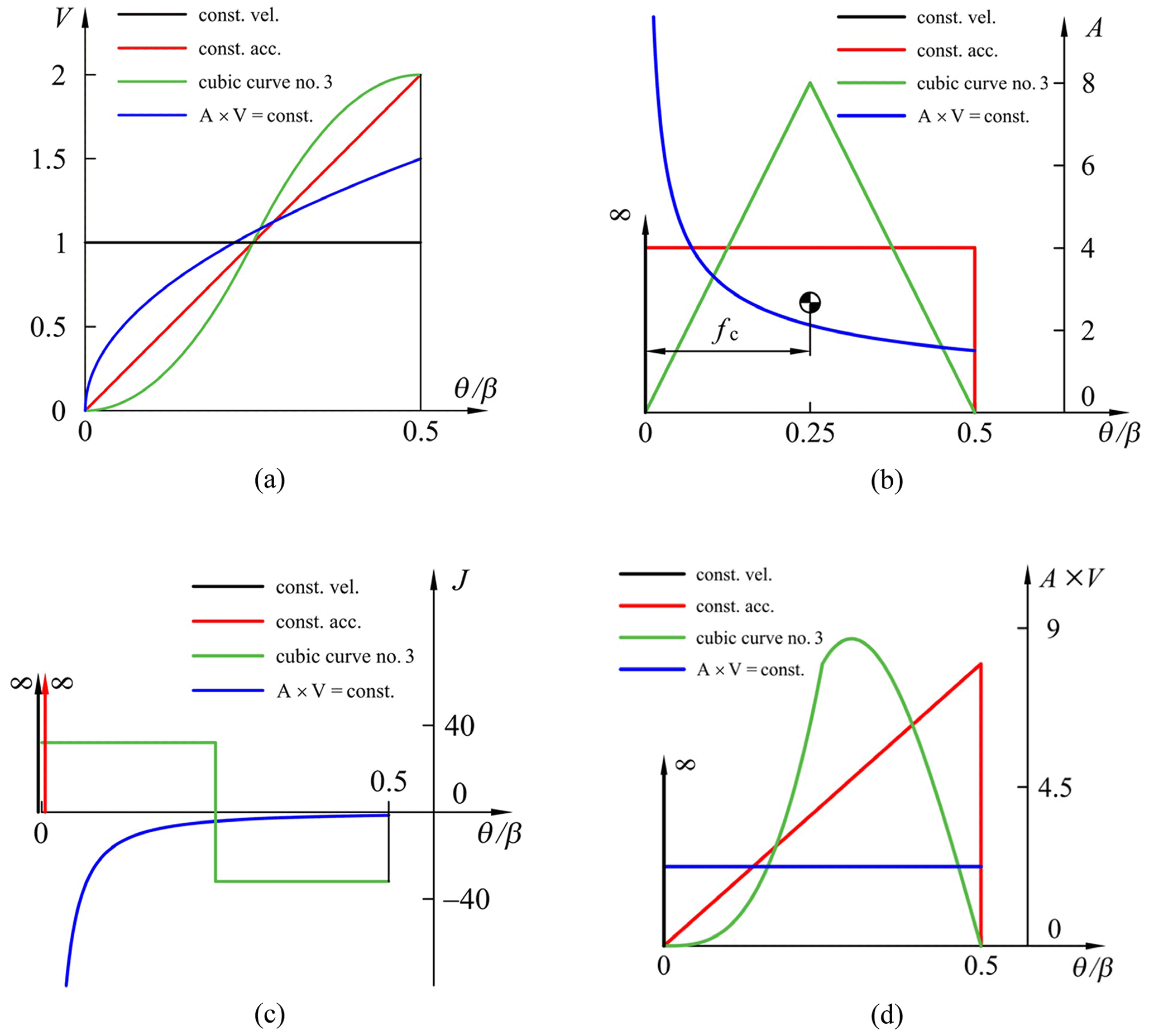
Figure 1 illustrates the normalized V, A, J, and A×V functions for four conventional motions. Neklutin (1969) suggests that the position of the centroid of each normalized acceleration function (denoted by f_c) will affect the values of motion characteristics. Decreasing the f_c will reduce the value of C_V, which can be verified in Table 1. In addition, the value of C_V equals 2 if f_c=0.25, such as the one of cubic curve no. 3 (labeled in Fig. 1b). Therefore, to lower the value of C_V, the position of f_c should be as close as the beginning of the acceleration function. On the other hand, smoothing the top of the acceleration function is helpful in reducing the value of C_A. Similarly, the value of C_J can be diminished by smoothing the top of the jerk function.

However, these dimensionless coefficients may not fall off simultaneously without a decision to compromise. In addition, velocity, acceleration, and jerk function are governed by the mathematical relationships of the derivative or integral. Any two of them are correspondingly determined once one of them has already been defined. Therefore, in synthesizing a motion program, it is suggested to deal with one function first, which is especially effective when beginning with its acceleration function. In doing so, motion characteristics of several conventional motions can be reduced.

3 Modified motion programs with better motion characteristics

For a family of trigonometric motion programs, such as cycloidal, modified sinusoidal, modified trapezoidal, and modified constant velocity 50 motion, their acceleration functions can be described by a generalized piecewise function. This piecewise acceleration function consists of constant segments and harmonically varying segments (Neklutin, 1969; Norton, 2009; Cheng, 2002). By editing the segment parameters, a family of trigonometric motion programs can be immediately obtained without extra tedious derivations. This model is universal but also takes its toll on the generality. The derived formulas are sort of lengthy because the whole motion program consists of multiple non-uniform expressions. In addition, since the whole motion is split into several pieces, the continuity at each end for every piecewise function should be carefully taken into consideration when this generalized modal is derived.

Figure 2 Comparison of two generalized phase angle functions.

Figure 3 The four phase angle functions in trigonometric motion.

This paper aims at characterizing the whole family of trigonometric motion programs by a uniform function. The proposed uniform function is used to describe the acceleration function for the whole family of trigonometric motion programs, which can be expressed as follows:

$$\begin{array}{}\text{(18)}& A\left(\mathit{\theta }\right)=C_{\mathrm{A}}{\displaystyle \frac{h}{{\mathit{\beta }}^{\mathrm{2}}}}\sin \left[\mathit{\varphi }\left(\mathit{\theta }\right)\right],\end{array}$$

where ϕ(θ) is the phase angle function in terms of cam rotation angle θ.

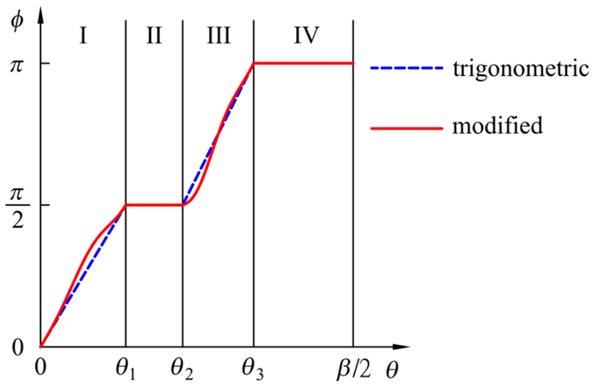
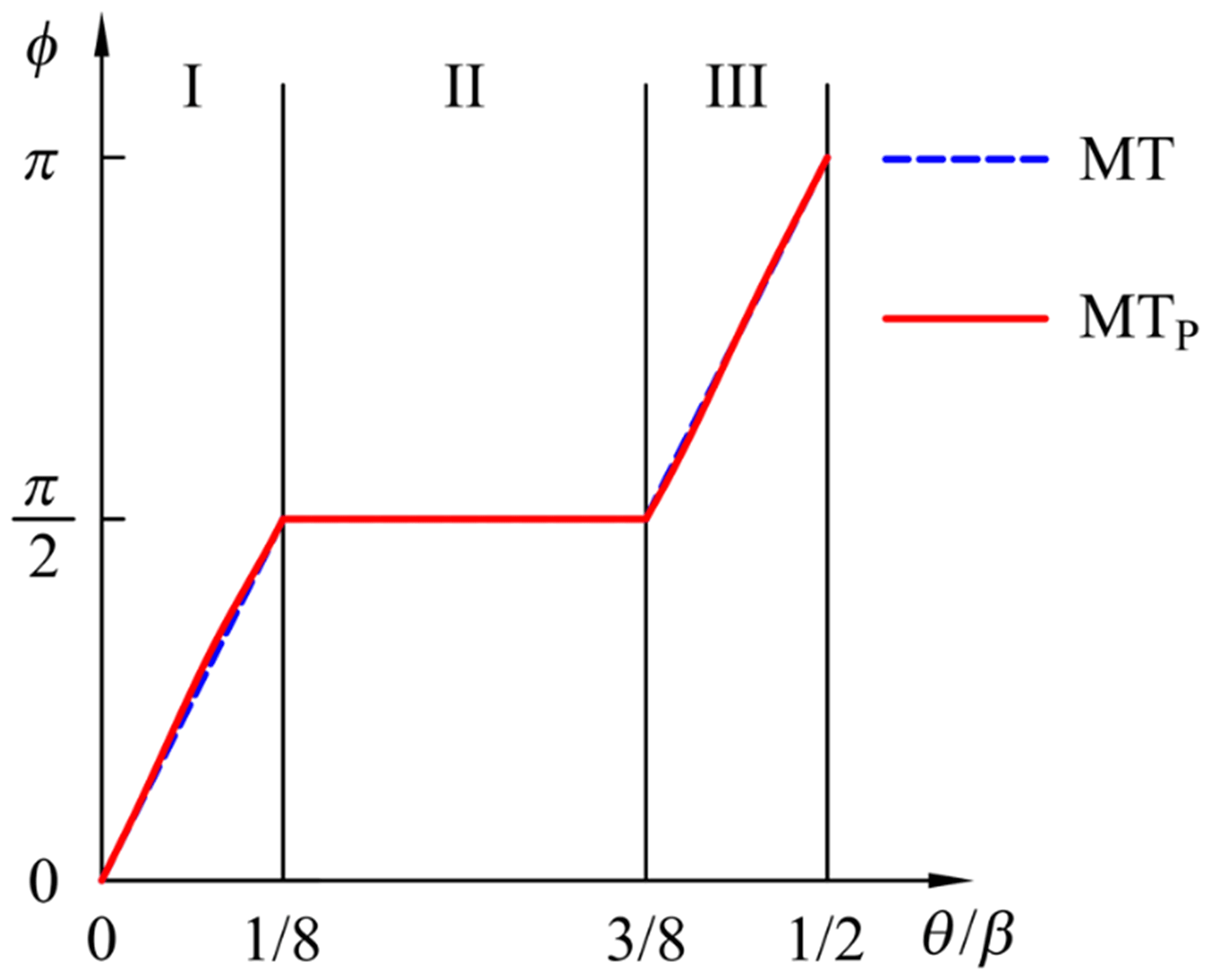
For the sake of simplicity, as explained above, the motion programs are only considered on the interval $[\mathrm{0},\mathit{\beta }/\mathrm{2}]$. To express the whole family of trigonometric motion programs by a uniform acceleration function, the phase angle function in the dashed line is divided into four zones, as shown in Fig. 2. The phase angle function in the first zone varies linearly from 0 to $\mathit{\pi }/\mathrm{2}$ and then stays constant during the second zone. The phase angle function linearly changes to π during the third zone and, finally, stays constant during the fourth zone.

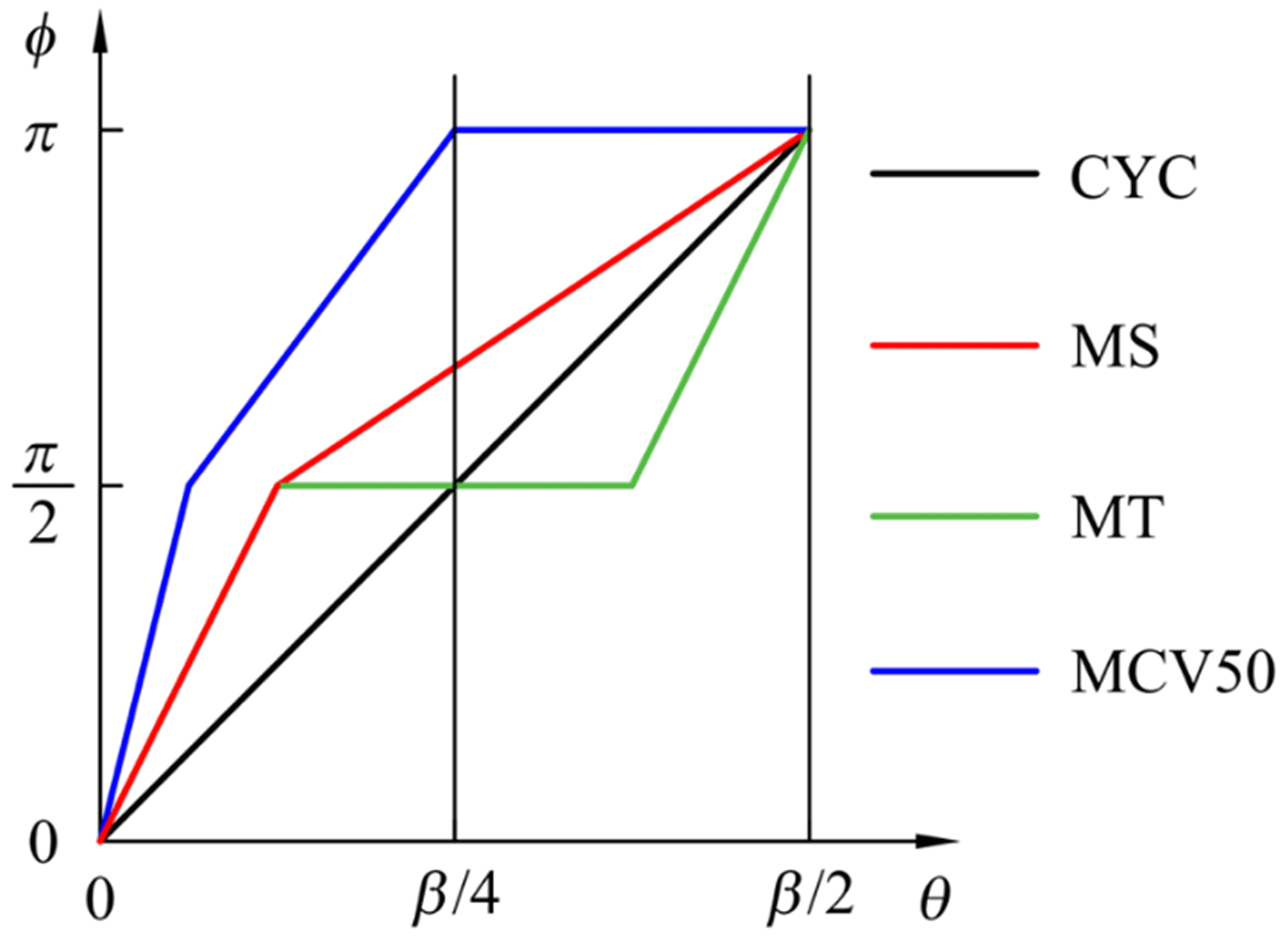
By specifically assigning the phase angle function, many commonly used motion programs can be obtained. For example, in reference to Fig. 3, a modified sinusoidal motion (MS) can be obtained by setting ${\mathit{\theta }}_{\mathrm{1}}={\mathit{\theta }}_{\mathrm{2}}=\mathit{\beta }/\mathrm{8}$ and ${\mathit{\theta }}_{\mathrm{3}}=\mathit{\beta }/\mathrm{2}$. If ${\mathit{\theta }}_{\mathrm{1}}={\mathit{\theta }}_{\mathrm{2}}=\mathit{\beta }/\mathrm{4}$ and ${\mathit{\theta }}_{\mathrm{3}}=\mathit{\beta }/\mathrm{2}$, a cycloidal motion (CYC) is obtained. If ${\mathit{\theta }}_{\mathrm{1}}=\mathit{\beta }/\mathrm{8}$, ${\mathit{\theta }}_{\mathrm{2}}=\mathrm{3}\mathit{\beta }/\mathrm{8}$, and ${\mathit{\theta }}_{\mathrm{3}}=\mathit{\beta }/\mathrm{2}$, a modified trapezoidal motion (MT) is obtained. If ${\mathit{\theta }}_{\mathrm{1}}={\mathit{\theta }}_{\mathrm{2}}=\mathit{\beta }/\mathrm{16}$ and ${\mathit{\theta }}_{\mathrm{3}}=\mathit{\beta }/\mathrm{4}$, a modified constant velocity 50 motion (MCV50) is obtained.

With reference to Fig. 3, three interesting facts can be observed. First, for these commonly used motion programs, their phase angle functions are linear in all zones. Second, the motion with a steeper phase angle function ϕ(θ) in zone I may have a f_c closer to the beginning of the stroke. Third, the top of the acceleration function will be smoother if the phase angle function ϕ(θ) around $\mathit{\theta }=\mathit{\beta }/\mathrm{4}$ has a smaller slope. The modified trapezoidal motion has a flat top of the acceleration function since its ϕ(θ) remains constant for one-quarter of the segment width of cam angle β. In light of the above reasoning, this paper proposes an alternative phase angle function aiming to reduce C_V, C_A, C_J, and C_M simultaneously. The proposed phase angle function is graphically illustrated with a solid line in Fig. 2. The expressions for the proposed phase angle function within each other zone are as follows:

$$\begin{array}{}\text{(19)}& {\displaystyle }\begin{array}{rl}& \text{I:}\mathrm{0}\le \mathit{\theta }\le {\mathit{\theta }}_{\mathrm{1}}\\ & \mathit{\varphi }\left(\mathit{\theta }\right)={\displaystyle \frac{\mathit{\pi }}{\mathrm{2}{\mathit{\theta }}_{\mathrm{1}}}}\mathit{\theta }+C_{\mathrm{1}}{\displaystyle \frac{\mathit{\pi }}{{\mathit{\theta }}_{\mathrm{1}}}}\mathit{\theta }[\mathrm{1}-\cos \left({\displaystyle \frac{\mathrm{2}\mathit{\pi }}{{\mathit{\theta }}_{\mathrm{1}}}}\mathit{\theta }\right)]\end{array}\text{(20)}& {\displaystyle }\begin{array}{rl}& \text{II:}{\mathit{\theta }}_{\mathrm{1}}\le \mathit{\theta }\le {\mathit{\theta }}_{\mathrm{2}}\\ & \mathit{\varphi }\left(\mathit{\theta }\right)={\displaystyle \frac{\mathit{\pi }}{\mathrm{2}}}\end{array}\text{(21)}& {\displaystyle }\begin{array}{rl}& \text{III:}{\mathit{\theta }}_{\mathrm{2}}\le \mathit{\theta }\le {\mathit{\theta }}_{\mathrm{3}}\\ & \mathit{\varphi }\left(\mathit{\theta }\right)={\displaystyle \frac{\mathit{\pi }\left({\mathit{\theta }}_{\mathrm{3}}-\mathrm{2}{\mathit{\theta }}_{\mathrm{2}}+\mathit{\theta }\right)}{\mathrm{2}({\mathit{\theta }}_{\mathrm{3}}-{\mathit{\theta }}_{\mathrm{2}})}}-{\displaystyle \frac{C_{\mathrm{2}}\mathit{\pi }\left({\mathit{\theta }}_{\mathrm{3}}-\mathit{\theta }\right)}{{\mathit{\theta }}_{\mathrm{3}}-{\mathit{\theta }}_{\mathrm{2}}}}\\ & \cdot \left[\sin \left(\mathrm{2}\mathit{\pi }{\displaystyle \frac{\mathit{\theta }-{\mathit{\theta }}_{\mathrm{2}}}{{\mathit{\theta }}_{\mathrm{3}}-{\mathit{\theta }}_{\mathrm{2}}}}\right)\right]\end{array}\text{(22)}& {\displaystyle }\begin{array}{rl}& \text{IV:}{\mathit{\theta }}_{\mathrm{3}}\le \mathit{\theta }\le {\displaystyle \frac{\mathit{\beta }}{\mathrm{2}}}\\ & \mathit{\varphi }\left(\mathit{\theta }\right)=\mathit{\pi },\end{array}\end{array}$$

where C₁ and C₂ are arbitrary coefficients, depending on the designer's options.

To provide constant acceleration segments, the proposed phase angle functions for both zone II and zone IV, expressed as Eqs. (20) and (22), are assumed to be constant. The nonlinear phase angle function in zone I aims to yield a closer f_c to the beginning of the acceleration function. Furthermore, the linear phase angle function in zone I, $\mathit{\pi }\mathit{\theta }/\mathrm{2}{\mathit{\theta }}_{\mathrm{1}}$, is combined with a nonlinear term, $C_{\mathrm{1}}\mathit{\pi }\mathit{\theta }/{\mathit{\theta }}_{\mathrm{1}}[\mathrm{1}-\mathrm{2}\cos (\mathrm{2}\mathit{\pi }\mathit{\theta }/{\mathit{\theta }}_{\mathrm{1}}\left)\right]$. The shape of this nonlinear term resembles that of the velocity function for cycloidal motion. Besides, to provide a steeper slope of the phase angle function, the amplitude of the nonlinear term is manipulated such that it increases as θ proceeds. As for the nonlinear phase angle function in zone III, the linear term, $\mathit{\pi }({\mathit{\theta }}_{\mathrm{3}}-\mathrm{2}{\mathit{\theta }}_{\mathrm{2}}+\mathit{\theta })/\mathrm{2}({\mathit{\theta }}_{\mathrm{3}}-{\mathit{\theta }}_{\mathrm{2}})$, is combined with a nonlinear term, $-C_{\mathrm{2}}\mathit{\pi }({\mathit{\theta }}_{\mathrm{3}}-\mathit{\theta })/({\mathit{\theta }}_{\mathrm{3}}-{\mathit{\theta }}_{\mathrm{2}})\mathit{\left\{}\sin \right[\mathrm{2}\mathit{\pi }(\mathit{\theta }-{\mathit{\theta }}_{\mathrm{2}})/({\mathit{\theta }}_{\mathrm{3}}-{\mathit{\theta }}_{\mathrm{2}})\left]\mathit{\right\}}$. The negative sine term wrapped around the linear slope in zone III can prevent the slope of the phase angle function from changing suddenly such that the top of the acceleration and jerk function will be smoother.

Once the values of θ₁, θ₂, θ₃, C₁, and C₂ are selected, the next step is to determine the preliminarily unknown coefficient C_A (Chen, 1969, 1972). By numerically integrating Eq. (18), a scaled displacement function multiplied with the coefficient C_A can be obtained. At last, the value of C_A can be directly solved by meeting the boundary condition for a prescribed stroke $S(\mathit{\beta }/\mathrm{2})=h/\mathrm{2}$. With the derived acceleration function, velocity and the displacement functions can be obtained by integrating the given acceleration function numerically. Taking the derivative of the acceleration function can yield the jerk function.

4 Illustrative examples

Numerical examples are presented to illustrate the application of the proposed phase angle function for the synthesis of new motion programs. To estimate the reduction in motion characteristics, commonly used trigonometric motions are also included in the following analysis to serve as the basis for the comparison.

Figure 4 Variation in phase angle function in Example 1.

Figure 5 Variation in normalized motion program in Example 1.

Table 2 Motion characteristics of CYC_P and CYC.

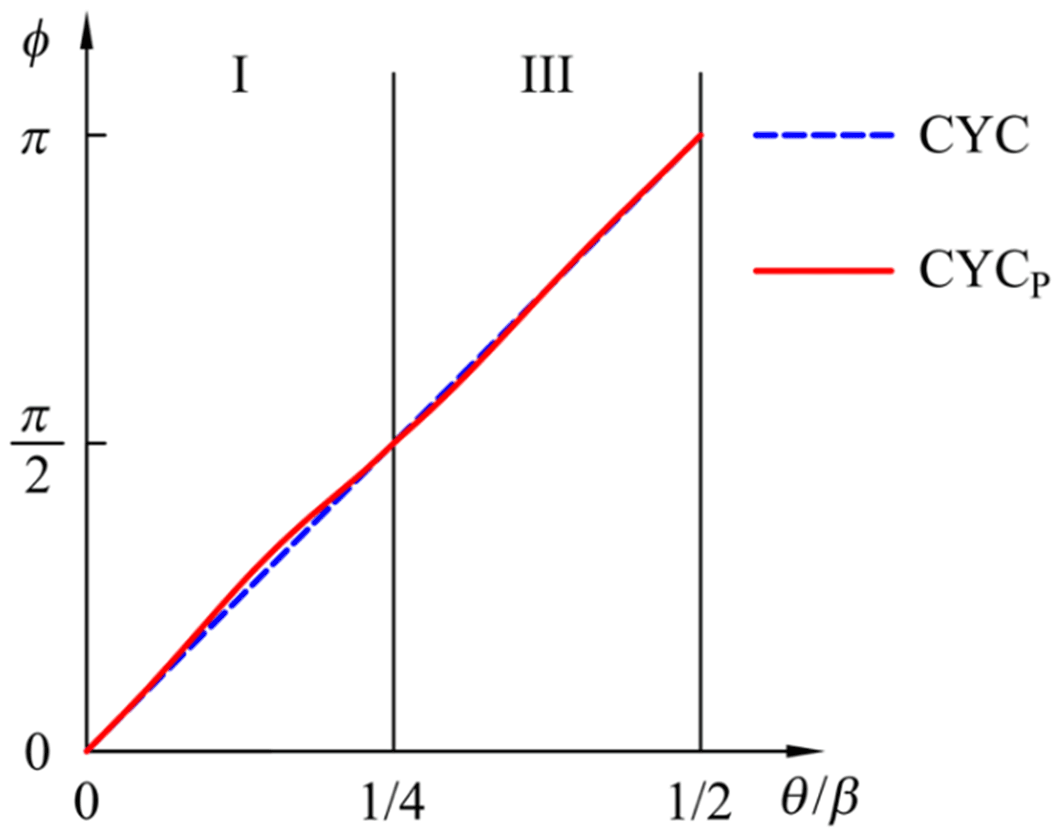
Example 1. Suppose that a motion program is synthesized by setting ${\mathit{\theta }}_{\mathrm{1}}={\mathit{\theta }}_{\mathrm{2}}=\mathit{\beta }/\mathrm{4}$, ${\mathit{\theta }}_{\mathrm{3}}=\mathit{\beta }/\mathrm{2}$, and coefficients $C_{\mathrm{1}}=\mathrm{1}/\mathrm{50}$ and $C_{\mathrm{2}}=\mathrm{1}/\mathrm{100}$. The zone arrangements of the synthesized motion program meet the same specification for the cycloidal motion (CYC). Once these design parameters are specified, the trapezoidal rule is adopted for approximating the scaled displacement function. Then, a solution satisfying the boundary condition $(\mathit{\theta },S)=(\mathit{\beta }/\mathrm{2},h/\mathrm{2})$ gives the value of C_A equal to 6.14. Thus, the varying acceleration functions of the synthesized motion program can be expressed as follows:

$$\begin{array}{}\text{(23)}& {\displaystyle }\begin{array}{rl}& \text{I:}\mathrm{0}\le \mathit{\theta }\le {\displaystyle \frac{\mathit{\beta }}{\mathrm{4}}}\\ & S^{\prime \prime }\left(\mathit{\theta }\right)=\mathrm{6.14}{\displaystyle \frac{h}{{\mathit{\beta }}^{\mathrm{2}}}}\sin [{\displaystyle \frac{\mathrm{52}\mathit{\pi }\mathit{\theta }}{\mathrm{25}\mathit{\beta }}}-{\displaystyle \frac{\mathrm{2}\mathit{\pi }\mathit{\theta }}{\mathrm{25}\mathit{\beta }}}\cos \left({\displaystyle \frac{\mathrm{8}\mathit{\pi }\mathit{\theta }}{\mathit{\beta }}}\right)]\end{array}\text{(24)}& {\displaystyle }\begin{array}{rl}& \text{III:}{\displaystyle \frac{\mathit{\beta }}{\mathrm{4}}}\le \mathit{\theta }\le {\displaystyle \frac{\mathit{\beta }}{\mathrm{2}}}\\ & S^{\prime \prime }\left(\mathit{\theta }\right)=\mathrm{6.14}{\displaystyle \frac{h}{{\mathit{\beta }}^{\mathrm{2}}}}\sin [{\displaystyle \frac{\mathrm{2}\mathit{\pi }\mathit{\theta }}{\mathit{\beta }}}-\left({\displaystyle \frac{\mathit{\pi }}{\mathrm{50}}}-{\displaystyle \frac{\mathit{\pi }\mathit{\theta }}{\mathrm{25}\mathit{\beta }}}\right)\\ & \cdot \sin \left({\displaystyle \frac{\mathrm{8}\mathit{\pi }\mathit{\theta }}{\mathit{\beta }}}\right)].\end{array}\end{array}$$

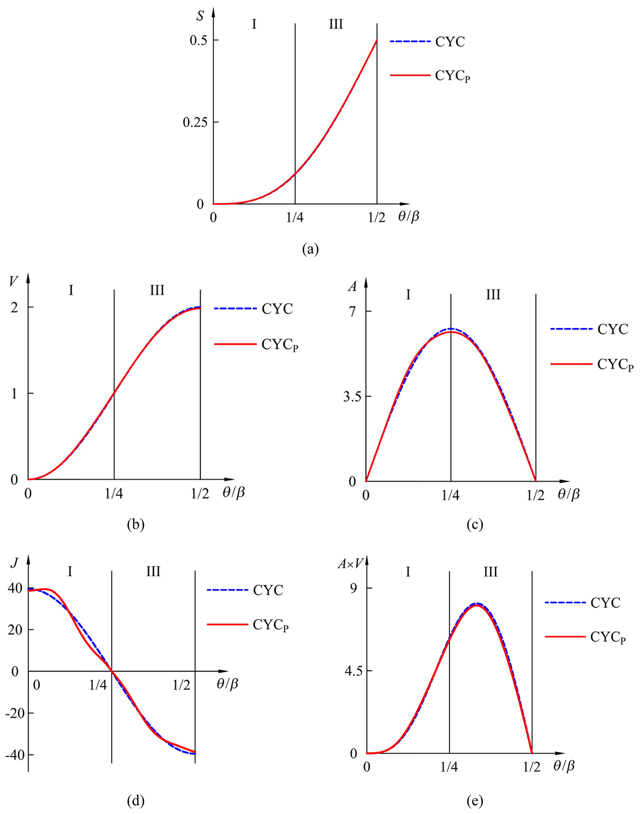
The phase angle functions are plotted in Fig. 4, and normalized S, V, A, J, and A×V functions are illustrated in Fig. 5. The synthesized motion (CYC_P) is a solid line, and the cycloidal motion (CYC) is a dashed line. The motion characteristics of the corresponding functions are listed in Table 2. Notice that the value f_c of synthesized motion CYC_P is smaller than that of cycloidal motion. The acceleration function of CYC_P is flatter at top interval. The jerk function also performs smooth connections at θ=0, $\mathit{\theta }=\mathit{\beta }/\mathrm{4}$, and $\mathit{\theta }=\mathit{\beta }/\mathrm{2}$. Table 2 indicates that these dimensionless coefficients C_V, C_A, C_J, and C_M fall slightly by applying the proposed phase angle function, and the average reduction in the motion characteristics is 1.36 %.

Figure 6 Variation in phase angle function in Example 2.

Figure 7 Variation in normalized motion program in Example 2.

Table 3 Motion characteristics of MS_P and MS.

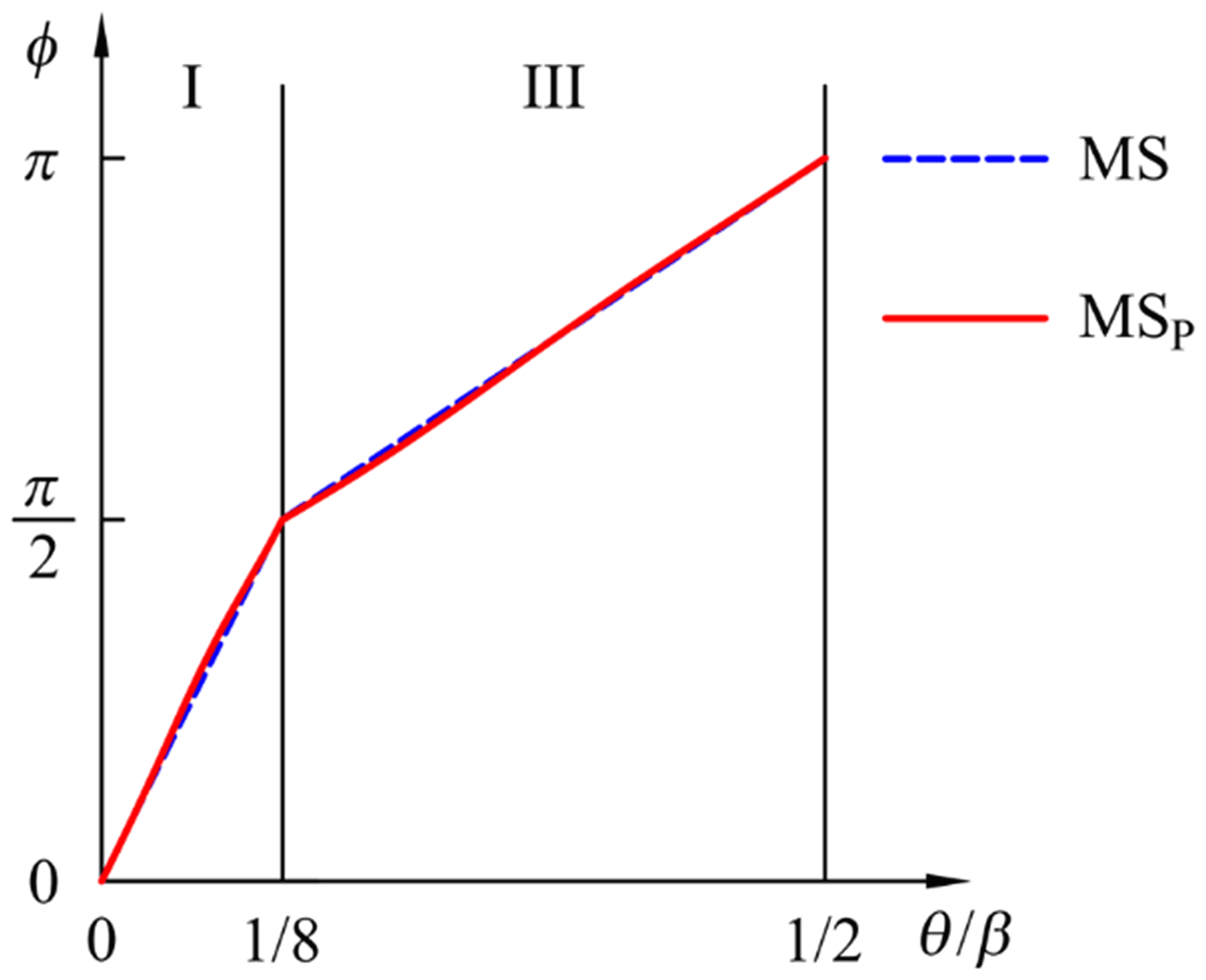
Example 2. Suppose that ${\mathit{\theta }}_{\mathrm{1}}={\mathit{\theta }}_{\mathrm{2}}=\mathit{\beta }/\mathrm{8}$, ${\mathit{\theta }}_{\mathrm{3}}=\mathit{\beta }/\mathrm{2}$, and coefficients $C_{\mathrm{1}}=\mathrm{1}/\mathrm{60}$ and $C_{\mathrm{2}}=\mathrm{1}/\mathrm{100}$. In doing so, the zone arrangements of the synthesized motion program meet the same specification as for modified sinusoidal motion (MS), which is regarded as the most widely used and is recommended as the standard motion program for general purposes (Norton, 2009; Tsay and Huey, 1989; Sandgren and West, 1989). With these design parameters specified, the derived value of C_A is equal to 5.47. Thus, the varying acceleration functions of the synthesized motion program can be expressed as follows:

$$\begin{array}{}\text{(25)}& {\displaystyle }\begin{array}{rl}& \text{I:}\mathrm{0}\le \mathit{\theta }\le {\displaystyle \frac{\mathit{\beta }}{\mathrm{8}}}\\ & S^{\prime \prime }\left(\mathit{\theta }\right)=\mathrm{5.47}{\displaystyle \frac{h}{{\mathit{\beta }}^{\mathrm{2}}}}\sin [{\displaystyle \frac{\mathrm{62}\mathit{\pi }\mathit{\theta }}{\mathrm{15}\mathit{\beta }}}-{\displaystyle \frac{\mathrm{2}\mathit{\pi }\mathit{\theta }}{\mathrm{15}\mathit{\beta }}}\cos \left({\displaystyle \frac{\mathrm{16}\mathit{\pi }\mathit{\theta }}{\mathit{\beta }}}\right)]\end{array}\text{(26)}& {\displaystyle }\begin{array}{rl}& \text{III}:{\displaystyle \frac{\mathit{\beta }}{\mathrm{8}}}\le \mathit{\theta }\le {\displaystyle \frac{\mathit{\beta }}{\mathrm{2}}}\\ & S^{\prime \prime }\left(\mathit{\theta }\right)=\mathrm{5.47}{\displaystyle \frac{h}{{\mathit{\beta }}^{\mathrm{2}}}}\sin [{\displaystyle \frac{\mathit{\pi }}{\mathrm{3}}}+{\displaystyle \frac{\mathrm{4}\mathit{\pi }\mathit{\theta }}{\mathrm{3}\mathit{\beta }}}-\left({\displaystyle \frac{\mathit{\pi }}{\mathrm{75}}}-{\displaystyle \frac{\mathrm{2}\mathit{\pi }\mathit{\theta }}{\mathrm{75}\mathit{\beta }}}\right)\\ & \cdot \sin \left({\displaystyle \frac{\mathrm{16}\mathit{\pi }\mathit{\theta }}{\mathrm{3}\mathit{\beta }}}-{\displaystyle \frac{\mathrm{2}\mathit{\pi }}{\mathrm{3}}}\right)].\end{array}\end{array}$$

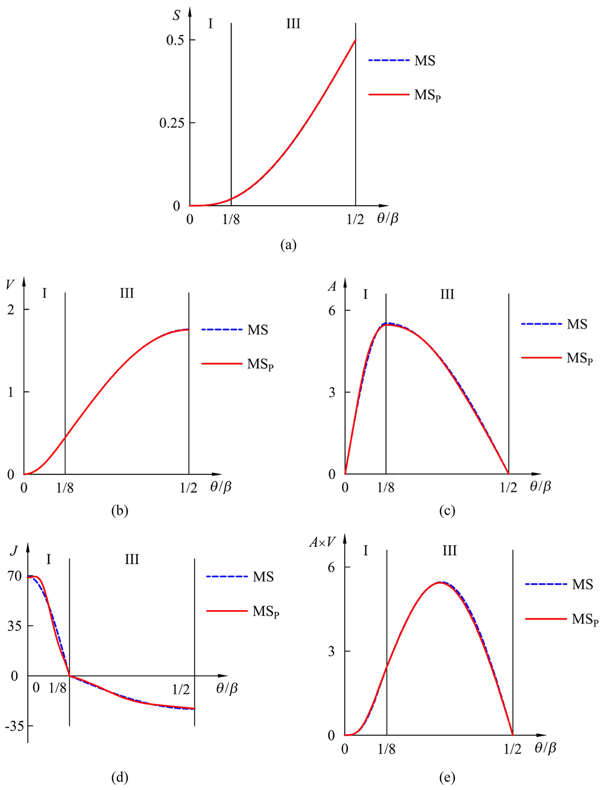
The phase functions are plotted in Fig. 6. The normalized S, V, A, J, and A×V functions are illustrated in Fig. 7. The synthesized motion (MS_P) is a solid line, and the modified sinusoidal motion (MS) is a dashed line. The motion characteristics of the corresponding functions are listed in Table 3. The top interval of acceleration function is smoother. Similar improvements also can be found at θ=0, $\mathit{\theta }=\mathit{\beta }/\mathrm{8}$, and $\mathit{\theta }=\mathit{\beta }/\mathrm{2}$ in the jerk function. Table 3 shows that the proposed phase angle function helps reduce these dimensionless coefficients of C_V, C_A, C_J, and C_M, whose average reduction in characteristic value is 0.64 %.

Figure 8 Variation in phase angle function in Example 3.

Figure 9 Variation in normalized motion program in Example 3.

Table 4 Motion characteristics of MT_P and MT.

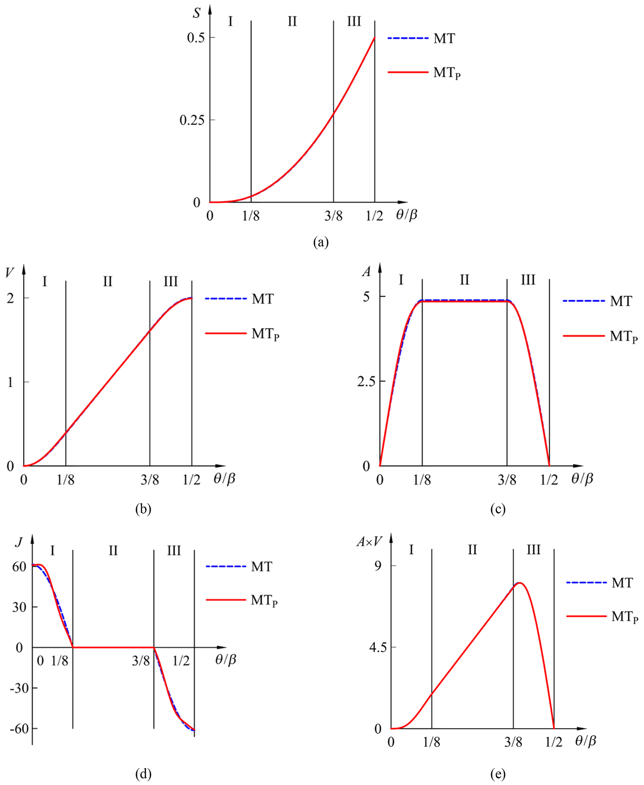
Example 3. In this example, a motion program which meets the same zone arrangements of modified trapezoidal motion is considered. The zones of the phase angle function are selected at ${\mathit{\theta }}_{\mathrm{1}}=\mathit{\beta }/\mathrm{8}$, ${\mathit{\theta }}_{\mathrm{2}}=\mathrm{3}\mathit{\beta }/\mathrm{8}$, ${\mathit{\theta }}_{\mathrm{3}}=\mathit{\beta }/\mathrm{2}$, and coefficients $C_{\mathrm{1}}=\mathrm{1}/\mathrm{70}$ and $C_{\mathrm{2}}=\mathrm{1}/\mathrm{100}$. Correspondingly, the characteristic value C_A is 4.85. Thus, the varying acceleration functions of the synthesized motion program can be expressed as follows:

$$\begin{array}{}\text{(27)}& {\displaystyle }\begin{array}{rl}& \text{I:}\mathrm{0}\le \mathit{\theta }\le {\displaystyle \frac{\mathit{\beta }}{\mathrm{8}}}\\ & S^{\prime \prime }\left(\mathit{\theta }\right)=\mathrm{4.85}{\displaystyle \frac{h}{{\mathit{\beta }}^{\mathrm{2}}}}\sin [{\displaystyle \frac{\mathrm{144}\mathit{\pi }\mathit{\theta }}{\mathrm{35}\mathit{\beta }}}-{\displaystyle \frac{\mathrm{4}\mathit{\pi }\mathit{\theta }}{\mathrm{35}\mathit{\beta }}}\cos \left({\displaystyle \frac{\mathrm{16}\mathit{\pi }\mathit{\theta }}{\mathit{\beta }}}\right)]\end{array}\text{(28)}& {\displaystyle }\begin{array}{rl}& \text{II:}{\displaystyle \frac{\mathit{\beta }}{\mathrm{8}}}\le \mathit{\theta }\le {\displaystyle \frac{\mathrm{3}\mathit{\beta }}{\mathrm{8}}}\\ & S^{\prime \prime }\left(\mathit{\theta }\right)=\mathrm{4.85}{\displaystyle \frac{h}{{\mathit{\beta }}^{\mathrm{2}}}}\end{array}\text{(29)}& {\displaystyle }\begin{array}{rl}& \text{III:}{\displaystyle \frac{\mathit{\beta }}{\mathrm{8}}}\le \mathit{\theta }\le {\displaystyle \frac{\mathit{\beta }}{\mathrm{2}}}\\ & S^{\prime \prime }\left(\mathit{\theta }\right)=\mathrm{4.85}{\displaystyle \frac{h}{{\mathit{\beta }}^{\mathrm{2}}}}\sin [-{\displaystyle \frac{\mathrm{4}\mathit{\pi }\mathit{\theta }}{\mathit{\beta }}}+\left({\displaystyle \frac{\mathit{\pi }}{\mathrm{25}}}-{\displaystyle \frac{\mathrm{2}\mathit{\pi }\mathit{\theta }}{\mathrm{25}\mathit{\beta }}}\right)\\ & \cdot \sin \left({\displaystyle \frac{\mathrm{16}\mathit{\pi }\mathit{\theta }}{\mathrm{3}\mathit{\beta }}}\right)].\end{array}\end{array}$$

The phase functions are plotted in Fig. 8. The normalized S, V, A, J, and A×V functions are illustrated in Fig. 9. The synthesized motion (MT_P) is a solid line, and the modified trapezoidal motion (MT) is a dashed line. The motion characteristics of the corresponding functions are listed in Table 4. As expected, applying the proposed phase angle function contributes to the reduction in these dimensionless coefficients C_V, C_A, C_J, and C_M, whose average reduction is 0.51 %. However, the value f_c of the synthesized acceleration function does not appear to change much in comparison to the foregoing examples. This result reveals that there is a smaller reduction in the value of C_V.

Figure 10 Variation in phase angle function in Example 4.

Figure 11 Variation in normalized motion program in Example 4.

Table 5 Motion characteristics of MCV50_P and MCV50.

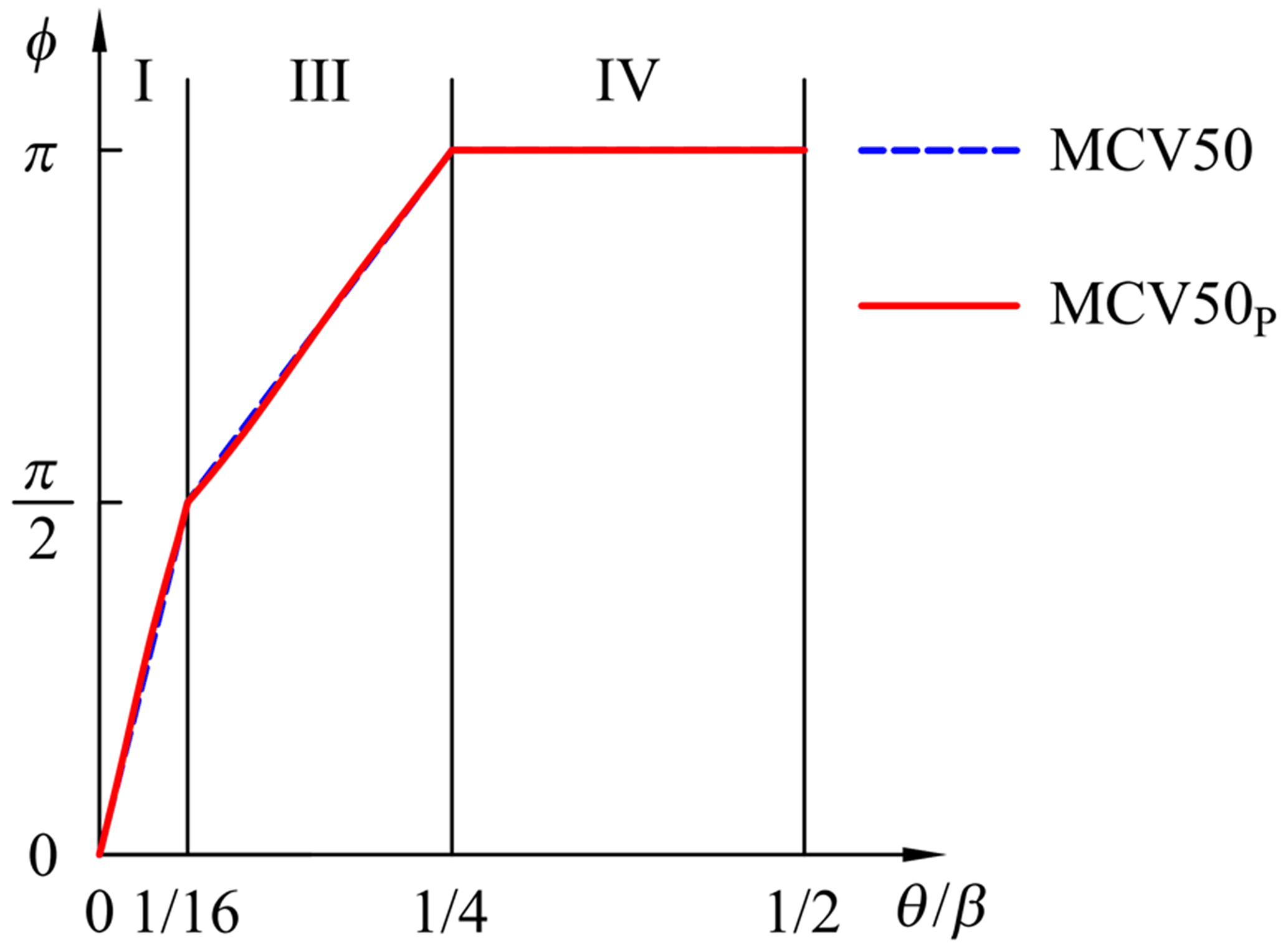
Example 4. The last example is to synthesize a motion program if its zone arrangements are identical to that of modified constant velocity 50 motion. The zones of the phase function are selected at ${\mathit{\theta }}_{\mathrm{1}}={\mathit{\theta }}_{\mathrm{2}}=\mathit{\beta }/\mathrm{16}$, ${\mathit{\theta }}_{\mathrm{3}}=\mathit{\beta }/\mathrm{4}$, and coefficients $C_{\mathrm{1}}=\mathrm{1}/\mathrm{65}$ and $C_{\mathrm{2}}=\mathrm{1}/\mathrm{100}$. Then, the characteristic value C_A is 7.95, which is solved by the aforementioned numerical computation. Thus, the varying acceleration functions of the synthesized motion program can be expressed as follows:

$$\begin{array}{}\text{(30)}& {\displaystyle }\begin{array}{rl}& \text{I:}\mathrm{0}\le \mathit{\theta }\le {\displaystyle \frac{\mathit{\beta }}{\mathrm{16}}}\\ & S^{\prime \prime }\left(\mathit{\theta }\right)=\mathrm{7.95}{\displaystyle \frac{h}{{\mathit{\beta }}^{\mathrm{2}}}}\sin [{\displaystyle \frac{\mathrm{536}\mathit{\pi }\mathit{\theta }}{\mathrm{65}\mathit{\beta }}}-{\displaystyle \frac{\mathrm{16}\mathit{\pi }\mathit{\theta }}{\mathrm{65}\mathit{\beta }}}\cos \left({\displaystyle \frac{\mathrm{32}\mathit{\pi }\mathit{\theta }}{\mathit{\beta }}}\right)]\end{array}\text{(31)}& {\displaystyle }\begin{array}{rl}& \text{III:}{\displaystyle \frac{\mathit{\beta }}{\mathrm{16}}}\le \mathit{\theta }\le {\displaystyle \frac{\mathit{\beta }}{\mathrm{4}}}\\ & S^{\prime \prime }\left(\mathit{\theta }\right)=\mathrm{7.95}{\displaystyle \frac{h}{{\mathit{\beta }}^{\mathrm{2}}}}\sin [{\displaystyle \frac{\mathit{\pi }}{\mathrm{3}}}+{\displaystyle \frac{\mathrm{8}\mathit{\pi }\mathit{\theta }}{\mathrm{3}\mathit{\beta }}}+\left({\displaystyle \frac{\mathit{\pi }}{\mathrm{75}}}-{\displaystyle \frac{\mathrm{4}\mathit{\pi }\mathit{\theta }}{\mathrm{75}\mathit{\beta }}}\right)\\ & \cdot \sin \left({\displaystyle \frac{\mathrm{32}\mathit{\pi }\mathit{\theta }}{\mathrm{3}\mathit{\beta }}}-{\displaystyle \frac{\mathrm{2}\mathit{\pi }}{\mathrm{3}}}\right)]\end{array}\text{(32)}& {\displaystyle }\begin{array}{rl}& \text{IV:}{\displaystyle \frac{\mathit{\beta }}{\mathrm{4}}}\le \mathit{\theta }\le {\displaystyle \frac{\mathit{\beta }}{\mathrm{2}}}\\ & S^{\prime \prime }\left(\mathit{\theta }\right)=\mathrm{0}.\end{array}\end{array}$$

The phase angle functions are plotted in Fig. 10. The normalized S, V, A, J, and A×V functions are illustrated in Fig. 11. The synthesized motion (MCV50_P) is a solid line, and modified constant velocity 50 motion (MCV50) is a dashed line. The motion characteristics of the corresponding functions are listed in Table 5. The average reduction in all motion characteristics is 0.30 %. Notice that the reduction percentage of the value f_c is quite close to that of Example 2. However, the reduction in the value of C_V is not as much as Example 2 yields. Besides, the value of C_M does not fall as expected in this example. The result suggests that the proposed phase angle function can be alternatively applied only by adopting the proposed phase angle function in zone I and keeping the other zones linear. Such a modified utilization may lead to a simultaneous reduction in these motion characteristics.

5 Discussion and remarks

Figure 12 illustrates the ratio of motion characteristics of synthesized motions to these of the corresponding trigonometric members. All motion characteristics, except for C_M of MCV50_P motion, fall down to a certain level. The reduction percentages range from 0.09 % to 2.22 %, and the average reduction in those values is 0.70 %. In addition, it can be further found that the reduction in motion characteristics in C_A and C_J, min is more significant than other coefficients.

Figure 12 Ratio of motion characteristics of synthesized motions to trigonometric motions.

Instead of being expressed as conventional piecewise functions, a family of trigonometric motion programs is characterized by a simplified and uniform function in this paper. The proposed function is in the form of a sinusoidal function used to describe the acceleration function. The acceleration function can be easily shaped by specifying the presented phase angle function to synthesize the desired trigonometric motion program. With the alternative phase angle function addressed in this paper, the maximum values of normalized velocity, acceleration, jerk, and acceleration multiplied by velocity of conventionally used trigonometric motions can be simultaneously reduced. From a kinematic point of view, a motion program with lower kinematic quantities is more preferable.