Low-harmonic trajectory synthesis using trajectory pattern method (TPM) for high-speed and high-precision machinery

In high-speed and high-precision machinery, trajectories with high-frequency harmonic content are one of the main sources of reduction of operational precision. Trajectories with high-frequency harmonic content generally demand even higher-harmonic actuating forces/torques due to the nonlinear dynamics of such systems, which may excite natural modes of vibration of the system and/or be beyond the dynamic response limitation of the actuation devices. In this paper, a global interpolation algorithm that uses the trajectory pattern method (TPM) for synthesizing low-harmonic trajectories is presented. The trajectory synthesis with the TPM is performed with a prescribed fundamental frequency and continuous jounce boundary condition, which would minimize the number of high-harmonic components in the required actuation forces/torques and avoid excitation of the system modes of vibration. The minimal curvature variation energy method, Lagrange multiplier method, and contour error control are used to obtain smooth kinematic profiles and satisfy the trajectory accuracy requirements. As an example, trajectory patterns that consist of a fundamental frequency sinusoidal time function and its first three harmonics are used to synthesize the desired trajectories for a selected dynamic system. The synthesized trajectories are shown to cause minimal system vibration during its operation. A comparison with a commonly used trajectory synthesis method clearly shows the superiority of the developed TPM-based approach in reducing vibration and demand on the actuator dynamic response, thereby allowing the system to operate at higher speeds and precision.

1 Introduction

For the trajectory synthesis (Chu et al., 2020; Dai et al., 2020; Van Loock et al., 2015) of high-speed machinery, such as CNC (computerized numerical control) machinery, robot manipulators and other computer-controlled machines, polynomial-based curves (Analooee et al., 2020; Liang and Su, 2019; Shen et al., 2020) are still the most widely used trajectories. It has the following advantages: (1) numerically stable algorithms; (2) it is more natural for designing and representing shape in a computer. The coefficients of functions possess considerable geometric significance. This translates into intuitive design methods. However, it is important to note that when expressed in Fourier series, all synthesized trajectories – such as those based on polynomial (Analooee et al., 2020; Shen et al., 2020), Akima (Bica, 2014; Wang et al., 2014), or B spline (Du et al., 2018; Simba et al., 2016) curves – contain significant high-harmonic content. In addition, the nonlinearity of the machine system dynamics would require actuating forces/torques with even higher-harmonic content to follow the prescribed trajectories. The lack of control over the harmonic content of the required actuating forces/torques and their frequencies in currently available and published methods for trajectory synthesis leads to excitation of natural modes of vibration of high-speed machinery.

In order to avoid exciting the natural modes of the mechanical structure or servo control system, many researchers have focused on flexible feed-rate planning methods for high-speed and high-precision machinery. Erkorkmaz and Altintas (2001) provided a continuous feed motion by constructing trapezoidal acceleration profiles along the quintic spline trajectory. Lee and Choi (2015) obtained smoother kinematic profiles with a discretized sinusoidal jerk function. To improve the flexibility, Wang (2015) proposed a trigonometric velocity scheduling algorithm, which could generate smooth velocity, acceleration, and jerk curves of parametric interpolation. Huang and Zhu (2016) represent jerk profiles by the sine series for feed-rate planning of parametric interpolator. The coefficients of the sine series are determined by selecting the geometric sequence. To reduce the time spent by the smoothing and planning process, Li et al. (2019) developed a real-time and look-ahead interpolation algorithm with axial jerk-smooth profiles. In one step, the algorithm finishes the trajectory synthesis and velocity planning by using the trigonometric velocity planning method. From these methods mentioned above, it can be seen that the vibration reduction effect is not obvious any more along with the increase of flexibility further, since the frequency distribution of synthesized kinematic profiles is not considered. The sine series method constructed jerk profiles with sinusoidal functions with an appropriate fundamental frequency and all harmonics, which contained considerable high-harmonic content. Although other methods did motion planning by using one sinusoidal function with a specified fundamental frequency, their velocity or/and displacement functions exist as polynomial items, which also results in significant high-harmonic components. Biagiotti and Melchiorri (2012) and Tajima et al. (2018) utilized finite impulse response filters to remove high-harmonic content of synthesized trajectories. However, filtering introduces unavoidable delay and induces large contouring errors in multi-axis motion that must be compensated since the filtered components are needed to achieve the prescribed motion.

Rastegar and Fardanesh (1990) introduced the concept of trajectory patterns that are constructed with sinusoidal functions with an appropriate fundamental frequency. Rastegar and Feng (2011) applied it to synthesis of trajectories with low-harmonic content such that the harmonic content of the required actuation forces/torques is controlled and does not contain significant high-harmonic content. The synthesized trajectory is a unique combination of a fundamental frequency harmonic and its second harmonic, which results in the minimum number of harmonics in the required actuation forces/torques and minimizes excitation of the system modes of vibrations. But this method is only used for point-to-point motions with zero end point velocity, acceleration, and jerk. To improve motion efficiency and precision, this paper, therefore, extends the trajectory pattern method (TPM) to construct trajectories with continuous velocity, acceleration, jerk, and jounce at mid-points. The fundamental frequency of the synthesized trajectories can be selected such that together with all its harmonics that appear in the trajectory and the required actuating forces/torques would not excite the natural modes of vibration of the system. The actuating forces/torques can then be readily optimized and used in a model-based control scheme to achieve high-speed and high-precision operation of the system.

In this paper, a path planning algorithm is presented that uses harmonic-based trajectory patterns for high-speed machinery. In Sect. 2, a global interpolation method using the TPM with a specified fundamental frequency, motion periods, and chord error is introduced. Minimal curvature variation energy and Lagrange multiplier method are used to synthesize the trajectories. The synthesized trajectories and axis kinematic profiles are smooth and only contain the fundamental frequency and its first three harmonics, which are designed to minimize vibration of the high-speed machinery. In Sect. 3, the effectiveness of the proposed algorithm is illustrated through computer simulations studies. Conclusions of the present study are presented in Sect. 4.

2 Low-harmonic trajectory patterns

In this section, a trajectory pattern method (TPM)-based global interpolation algorithm, which achieves smooth axis motion profiles with chord error constraint, is presented. In these profiles, trajectory patterns that are synthesized with a fundamental frequency and its first three harmonics are used to achieve minimum trajectory harmonic content (Rastegar and Feng, 2011).

2.1 Trajectory pattern

The class of trajectory patterns used in the present study is harmonic based and is formed by a fundamental sinusoidal function and (n−1) number of its harmonics:

$$\begin{array}{}\text{(1)}& g\left(t\right)=\sum _{i=\mathrm{0}}^n\left[a_i\cos \left(\mathrm{2}\mathit{\pi }ift\right)+b_i\sin \left(\mathrm{2}\mathit{\pi }ift\right)\right],n\in N,\end{array}$$

where a_i and b_i are trajectory parameters; t is the time, $t\in [\mathrm{0},T]$, and T is the motion period; f is the selected fundamental frequency of the trajectory pattern.

In the present study, the selected trajectory pattern used for trajectory synthesis consists of a fundamental frequency sinusoidal function and its first three harmonics. The displacement function is then expressed as

$$\begin{array}{}\text{(2)}& \begin{array}{rl}s\left(t\right)& =a_{\mathrm{0}}+a_{\mathrm{1}}\cos \left(\mathrm{2}\mathit{\pi }ft\right)+a_{\mathrm{2}}\cos \left(\mathrm{4}\mathit{\pi }ft\right)\\ & +a_{\mathrm{3}}\cos \left(\mathrm{6}\mathit{\pi }ft\right)+a_{\mathrm{4}}\cos \left(\mathrm{8}\mathit{\pi }ft\right)+b_{\mathrm{1}}\sin \left(\mathrm{2}\mathit{\pi }ft\right)\\ & +b_{\mathrm{2}}\sin \left(\mathrm{4}\mathit{\pi }ft\right)+b_{\mathrm{3}}\sin \left(\mathrm{6}\mathit{\pi }ft\right)+b_{\mathrm{4}}\sin \left(\mathrm{8}\mathit{\pi }ft\right).\end{array}\end{array}$$

From Eq. (2), the velocity, acceleration, jerk, and jounce functions are then derived as

$$\begin{array}{}\text{(3)}& {\displaystyle }\begin{array}{rl}v\left(t\right)& =-\mathrm{2}\mathit{\pi }f{a}_{\mathrm{1}}\sin \left(\mathrm{2}\mathit{\pi }ft\right)-\mathrm{4}\mathit{\pi }f{a}_{\mathrm{2}}\sin \left(\mathrm{4}\mathit{\pi }ft\right)\\ & -\mathrm{6}\mathit{\pi }f{a}_{\mathrm{3}}\sin \left(\mathrm{6}\mathit{\pi }ft\right)-\mathrm{8}\mathit{\pi }f{a}_{\mathrm{4}}\sin \left(\mathrm{8}\mathit{\pi }ft\right)\\ & +\mathrm{2}\mathit{\pi }f{b}_{\mathrm{1}}\cos \left(\mathrm{2}\mathit{\pi }ft\right)+\mathrm{4}\mathit{\pi }f{b}_{\mathrm{2}}\cos \left(\mathrm{4}\mathit{\pi }ft\right)\\ & +\mathrm{6}\mathit{\pi }f{b}_{\mathrm{3}}\cos \left(\mathrm{6}\mathit{\pi }ft\right)+\mathrm{8}\mathit{\pi }f{b}_{\mathrm{4}}\cos \left(\mathrm{8}\mathit{\pi }ft\right)\end{array}\text{(4)}& {\displaystyle }\begin{array}{rl}a\left(t\right)& =-\left(\mathrm{2}\mathit{\pi }f{)}^{\mathrm{2}}{a}_{\mathrm{1}}\cos \right(\mathrm{2}\mathit{\pi }ft)-(\mathrm{4}\mathit{\pi }f{)}^{\mathrm{2}}{a}_{\mathrm{2}}\cos \left(\mathrm{4}\mathit{\pi }ft\right)\\ & -\left(\mathrm{6}\mathit{\pi }f{)}^{\mathrm{2}}{a}_{\mathrm{3}}\cos \right(\mathrm{6}\mathit{\pi }ft)-(\mathrm{8}\mathit{\pi }f{)}^{\mathrm{2}}{a}_{\mathrm{4}}\cos \left(\mathrm{8}\mathit{\pi }ft\right)\\ & -\left(\mathrm{2}\mathit{\pi }f{)}^{\mathrm{2}}{b}_{\mathrm{1}}\sin \right(\mathrm{2}\mathit{\pi }ft)-(\mathrm{4}\mathit{\pi }f{)}^{\mathrm{2}}{b}_{\mathrm{2}}\sin \left(\mathrm{4}\mathit{\pi }ft\right)\\ & -\left(\mathrm{6}\mathit{\pi }f{)}^{\mathrm{2}}{b}_{\mathrm{3}}\sin \right(\mathrm{6}\mathit{\pi }ft)-(\mathrm{8}\mathit{\pi }f{)}^{\mathrm{2}}{b}_{\mathrm{4}}\sin \left(\mathrm{8}\mathit{\pi }ft\right)\end{array}\text{(5)}& {\displaystyle }\begin{array}{rl}j\left(t\right)& =\left(\mathrm{2}\mathit{\pi }f{)}^{\mathrm{3}}{a}_{\mathrm{1}}\sin \right(\mathrm{2}\mathit{\pi }ft)+(\mathrm{4}\mathit{\pi }f{)}^{\mathrm{3}}{a}_{\mathrm{2}}\sin \left(\mathrm{4}\mathit{\pi }ft\right)\\ & +\left(\mathrm{6}\mathit{\pi }f{)}^{\mathrm{3}}{a}_{\mathrm{3}}\sin \right(\mathrm{6}\mathit{\pi }ft)+(\mathrm{8}\mathit{\pi }f{)}^{\mathrm{3}}{a}_{\mathrm{4}}\sin \left(\mathrm{8}\mathit{\pi }ft\right)\\ & -\left(\mathrm{2}\mathit{\pi }f{)}^{\mathrm{3}}{b}_{\mathrm{1}}\cos \right(\mathrm{2}\mathit{\pi }ft)-(\mathrm{4}\mathit{\pi }f{)}^{\mathrm{3}}{b}_{\mathrm{2}}\cos \left(\mathrm{4}\mathit{\pi }ft\right)\\ & -\left(\mathrm{6}\mathit{\pi }f{)}^{\mathrm{3}}{b}_{\mathrm{3}}\cos \right(\mathrm{6}\mathit{\pi }ft)-(\mathrm{8}\mathit{\pi }f{)}^{\mathrm{3}}{b}_{\mathrm{4}}\cos \left(\mathrm{8}\mathit{\pi }ft\right)\end{array}\text{(6)}& {\displaystyle }\begin{array}{rl}jo\left(t\right)& =\left(\mathrm{2}\mathit{\pi }f{)}^{\mathrm{4}}{a}_{\mathrm{1}}\cos \right(\mathrm{2}\mathit{\pi }ft)+(\mathrm{4}\mathit{\pi }f{)}^{\mathrm{4}}{a}_{\mathrm{2}}\cos \left(\mathrm{4}\mathit{\pi }ft\right)\\ & +\left(\mathrm{6}\mathit{\pi }f{)}^{\mathrm{4}}{a}_{\mathrm{3}}\cos \right(\mathrm{6}\mathit{\pi }ft)+(\mathrm{8}\mathit{\pi }f{)}^{\mathrm{4}}{a}_{\mathrm{4}}\cos \left(\mathrm{8}\mathit{\pi }ft\right)\\ & +\left(\mathrm{2}\mathit{\pi }f{)}^{\mathrm{4}}{b}_{\mathrm{1}}\sin \right(\mathrm{2}\mathit{\pi }ft)+(\mathrm{4}\mathit{\pi }f{)}^{\mathrm{4}}{b}_{\mathrm{2}}\sin \left(\mathrm{4}\mathit{\pi }ft\right)\\ & +\left(\mathrm{6}\mathit{\pi }f{)}^{\mathrm{4}}{b}_{\mathrm{3}}\sin \right(\mathrm{6}\mathit{\pi }ft)+(\mathrm{8}\mathit{\pi }f{)}^{\mathrm{4}}{b}_{\mathrm{4}}\sin \left(\mathrm{8}\mathit{\pi }ft\right).\end{array}\end{array}$$

In the following sections, the present low-harmonic trajectory synthesis is presented by its application to a point-to-point trajectory synthesis. The method is however general and may be applied to other motion scenarios, for example for motions starting from rest and ending to start a constant velocity motion or from a constant velocity motion to a stop, a scenario that is very often encountered in high-speed and high-precision machine operations.

2.2 Low-harmonic trajectory synthesis for point-to-point motions

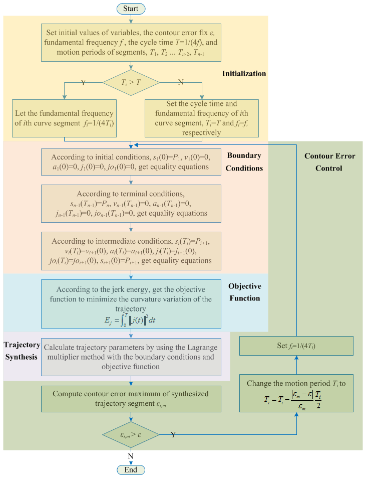
Figure 1 shows the flow diagram of the developed global interpolation algorithm. The trajectory synthesis includes five modules: an initialization module; a boundary conditions definition module; a jerk energy function definition module; a trajectory parameters calculation module; and a contour error control module. A Lagrange multiplier method is used to calculate the trajectory parameters with the indicated objective function and equality constraints. The above modules are described in more detail in the following sections.

Figure 1 Flowchart of the low-harmonic trajectory synthesis.

2.2.1 Initialization module

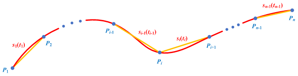
Figure 2 presents point-to-point motion from the point P₁ to the point P_n, which is divided into n−1 segments. In this example, the path segments are considered to line segments. The path of the point-to-point motion is therefore given by n number of data points, P₁, P₂ …P_n−1, P_n, and (n−1) number of segment trajectories s₁(t₁), s₂(t₂) …$s_{n-\mathrm{2}}\left(t_{n-\mathrm{2}}\right)$, $s_{n-\mathrm{1}}\left(t_{n-\mathrm{1}}\right)$ are to be synthesized. Here, n is a positive integer and n≥2, and t₁, t₂ …t_n−2, t_n−1 are trajectory segment times.

The user is to provide the required contour error ε, the motion period for each trajectory segment, T₁, T₂ …T_n−2, T_n−1, with $\mathrm{0}\le t_i\le T_i$, i=1, …, n−1, and the fundamental frequency f of the trajectory pattern for motion from P₁ to P_n, which must be selected such that together with its first three harmonics, the natural modes of vibration of the system are not excited.

To simplify the construction process and obtain continuous smooth axis motion profiles, the cycle time T is set equal to a quarter of the fundamental frequency period, i.e., $T=\mathrm{1}/\left(\mathrm{4}f\right)$.

For the trajectory segments, motion periods and corresponding fundamental frequencies f₁, f₂ …f_n−2, f_n−1 are adjusted to reduce the high-frequency harmonic content of the trajectory. In addition, for each trajectory segment, such as the segment P_iP_i+1, if T_i>T, we let $f_i=\mathrm{1}/\left(\mathrm{4}{T}_i\right)$; otherwise let T_i=T and f_i=f.

In Fig. 2, the trajectory segment curves are drawn in red and are shown to pass through the path segment ends P₁, P₂ …P_n−1, P_n with smooth kinematic profiles.

Figure 2 Path and synthesized trajectories.

2.2.2 Boundary conditions

To achieve continuous smooth axis motion profiles, boundary conditions are necessary. In addition, since the motion is point to point, the velocities, accelerations, jerks, and jounces at the start point P₁ and end point P_n−1 are set to zero. Then using Eqs. (2)–(6), the initial conditions of the first curve segment s₁(t₁) at t₁=0 are obtained as

$$\begin{array}{}\text{(7)}& {\displaystyle }{s}_{\mathrm{1}}\left(\mathrm{0}\right)=a_{\mathrm{1},\mathrm{0}}+a_{\mathrm{1},\mathrm{1}}+a_{\mathrm{1},\mathrm{2}}+a_{\mathrm{1},\mathrm{3}}+a_{\mathrm{1},\mathrm{4}}=P_{\mathrm{1}}\text{(8)}& {\displaystyle }{v}_{\mathrm{1}}\left(\mathrm{0}\right)=b_{\mathrm{1},\mathrm{1}}+\mathrm{2}{b}_{\mathrm{1},\mathrm{2}}+\mathrm{3}{b}_{\mathrm{1},\mathrm{3}}+\mathrm{4}{b}_{\mathrm{1},\mathrm{4}}=\mathrm{0}\text{(9)}& {\displaystyle }{a}_{\mathrm{1}}\left(\mathrm{0}\right)=a_{\mathrm{1},\mathrm{1}}+\mathrm{4}{a}_{\mathrm{1},\mathrm{2}}+\mathrm{9}{a}_{\mathrm{1},\mathrm{3}}+\mathrm{16}{a}_{\mathrm{1},\mathrm{4}}=\mathrm{0}\text{(10)}& {\displaystyle }{j}_{\mathrm{1}}\left(\mathrm{0}\right)=b_{\mathrm{1},\mathrm{1}}+\mathrm{8}{b}_{\mathrm{1},\mathrm{2}}+\mathrm{27}{b}_{\mathrm{1},\mathrm{3}}+\mathrm{64}{b}_{\mathrm{1},\mathrm{4}}=\mathrm{0}\text{(11)}& {\displaystyle }j{o}_{\mathrm{1}}\left(\mathrm{0}\right)=a_{\mathrm{1},\mathrm{1}}+\mathrm{16}{a}_{\mathrm{1},\mathrm{2}}+\mathrm{81}{a}_{\mathrm{1},\mathrm{3}}+\mathrm{256}{a}_{\mathrm{1},\mathrm{4}}=\mathrm{0}.\end{array}$$

Similarly, the terminal conditions of the last curve segment $s_{n-\mathrm{1}}\left(t_{n-\mathrm{1}}\right)$ at $t_{n-\mathrm{1}}=T_{n-\mathrm{1}}$ are expressed as

$$\begin{array}{}\text{(12)}& {\displaystyle }\begin{array}{rl}{s}_{n-\mathrm{1}}\left(T_{n-\mathrm{1}}\right)& =a_{n-\mathrm{1},\mathrm{0}}-a_{n-\mathrm{1},\mathrm{2}}+a_{n-\mathrm{1},\mathrm{4}}\\ & +b_{n-\mathrm{1},\mathrm{1}}-b_{n-\mathrm{1},\mathrm{3}}=P_n\end{array}\text{(13)}& {\displaystyle }\begin{array}{rl}{v}_{n-\mathrm{1}}\left(T_{n-\mathrm{1}}\right)& =-a_{n-\mathrm{1},\mathrm{1}}+\mathrm{3}{a}_{n-\mathrm{1},\mathrm{3}}\\ & -\mathrm{2}{b}_{n-\mathrm{1},\mathrm{2}}+\mathrm{4}{b}_{n-\mathrm{1},\mathrm{4}}=\mathrm{0}\end{array}\text{(14)}& {\displaystyle }\begin{array}{rl}{a}_{n-\mathrm{1}}\left(T_{n-\mathrm{1}}\right)& =\mathrm{4}{a}_{n-\mathrm{1},\mathrm{2}}-\mathrm{16}{a}_{n-\mathrm{1},\mathrm{4}}\\ & -b_{n-\mathrm{1},\mathrm{1}}+\mathrm{9}{a}_{n-\mathrm{1},\mathrm{3}}=\mathrm{0}\end{array}\text{(15)}& {\displaystyle }\begin{array}{rl}{j}_{n-\mathrm{1}}\left(T_{n-\mathrm{1}}\right)& =a_{n-\mathrm{1},\mathrm{1}}-\mathrm{27}{a}_{n-\mathrm{1},\mathrm{3}}\\ & +\mathrm{8}{b}_{n-\mathrm{1},\mathrm{2}}-\mathrm{64}{b}_{n-\mathrm{1},\mathrm{4}}=\mathrm{0}\end{array}\text{(16)}& {\displaystyle }\begin{array}{rl}j{o}_{n-\mathrm{1}}\left(T_{n-\mathrm{1}}\right)& =-\mathrm{16}{a}_{n-\mathrm{1},\mathrm{2}}+\mathrm{256}{a}_{n-\mathrm{1},\mathrm{4}}\\ & +b_{n-\mathrm{1},\mathrm{1}}-\mathrm{81}{b}_{n-\mathrm{1},\mathrm{3}}=\mathrm{0}.\end{array}\end{array}$$

In Fig. 2, for mid-points, P₂ …P_n−1, adjacent curve segments must have the same velocity, acceleration, jerk, and jounce at the nodes, that is

$$\begin{array}{}\text{(17)}& \left\{\begin{array}{l}{s}_i\left(T_i\right)=P_{i+\mathrm{1}}\\ v_i\left(T_i\right)=v_{i+\mathrm{1}}\left(\mathrm{0}\right)\\ a_i\left(T_i\right)=a_{i+\mathrm{1}}\left(\mathrm{0}\right)\\ j_i\left(T_i\right)=j_{i+\mathrm{1}}\left(\mathrm{0}\right)\\ j{o}_i\left(T_i\right)=j{o}_{i+\mathrm{1}}\left(\mathrm{0}\right)\\ s_{i+\mathrm{1}}\left(\mathrm{0}\right)=P_{i+\mathrm{1}}\\ i=\mathrm{1},\mathrm{\dots },n-\mathrm{2}\end{array}\right..\end{array}$$

Then substituting Eqs. (2)–(6) into Eq. (17), we can get

$$\begin{array}{}\text{(18)}& {\displaystyle }{a}_{i,\mathrm{0}}-a_{i,\mathrm{2}}+a_{i,\mathrm{4}}+b_{i,\mathrm{1}}-b_{i,\mathrm{3}}=P_{i+\mathrm{1}}\text{(19)}& {\displaystyle }\begin{array}{rl}& \mathrm{2}\mathit{\pi }{f}_i(a_{i,\mathrm{1}}-\mathrm{3}{a}_{i,\mathrm{3}}+\mathrm{2}{b}_{i,\mathrm{2}}-\mathrm{4}{b}_{i,\mathrm{4}})+\mathrm{2}\mathit{\pi }{f}_{i+\mathrm{1}}(b_{i+\mathrm{1},\mathrm{1}}\\ & +\mathrm{2}{b}_{i+\mathrm{1},\mathrm{2}}+\mathrm{3}{b}_{i+\mathrm{1},\mathrm{3}}+\mathrm{4}{b}_{i+\mathrm{1},\mathrm{4}})=\mathrm{0}\end{array}\text{(20)}& {\displaystyle }\begin{array}{rl}& \left(\mathrm{2}\mathit{\pi }{f}_i{)}^{\mathrm{2}}\right(\mathrm{4}{a}_{i,\mathrm{2}}-\mathrm{16}{a}_{i,\mathrm{4}}-b_{i,\mathrm{1}}+\mathrm{9}{b}_{i,\mathrm{3}})+(\mathrm{2}\mathit{\pi }{f}_i{)}^{\mathrm{2}}\\ & (a_{i+\mathrm{1},\mathrm{1}}+\mathrm{4}{a}_{i+\mathrm{1},\mathrm{2}}+\mathrm{9}{a}_{i+\mathrm{1},\mathrm{3}}+\mathrm{16}{a}_{i+\mathrm{1},\mathrm{4}})=\mathrm{0}\end{array}\text{(21)}& {\displaystyle }\begin{array}{rl}& \left(\mathrm{2}\mathit{\pi }{f}_i{)}^{\mathrm{3}}\right(a_{i,\mathrm{1}}-\mathrm{27}{a}_{i,\mathrm{3}}+\mathrm{8}{b}_{i,\mathrm{2}}-\mathrm{64}{b}_{i,\mathrm{4}})+(\mathrm{2}\mathit{\pi }{f}_i{)}^{\mathrm{3}}\\ & (b_{i+\mathrm{1},\mathrm{1}}+\mathrm{8}{b}_{i+\mathrm{1},\mathrm{2}}+\mathrm{27}{b}_{i+\mathrm{1},\mathrm{3}}+\mathrm{64}{b}_{i+\mathrm{1},\mathrm{4}})=\mathrm{0}\end{array}\text{(22)}& {\displaystyle }\begin{array}{rl}& \left(\mathrm{2}\mathit{\pi }{f}_i{)}^{\mathrm{4}}\right(\mathrm{16}{a}_{i,\mathrm{2}}-\mathrm{256}{a}_{i,\mathrm{4}}-b_{i,\mathrm{1}}+\mathrm{81}{b}_{i,\mathrm{3}})\\ & +\left(\mathrm{2}\mathit{\pi }{f}_i{)}^{\mathrm{4}}\right(a_{i+\mathrm{1},\mathrm{1}}+\mathrm{16}{a}_{i+\mathrm{1},\mathrm{2}}+\mathrm{81}{a}_{i+\mathrm{1},\mathrm{3}}\\ & +\mathrm{256}{a}_{i+\mathrm{1},\mathrm{4}})=\mathrm{0}\end{array}\text{(23)}& {\displaystyle }{a}_{i+\mathrm{1},\mathrm{0}}+a_{i+\mathrm{1},\mathrm{1}}+a_{i+\mathrm{1},\mathrm{2}}+a_{i+\mathrm{1},\mathrm{3}}+a_{i+\mathrm{1},\mathrm{4}}=P_{i+\mathrm{1}},\end{array}$$

where i=1, …, n−2.

2.2.3 Jerk energy function

The internal energy of curve segments can affect its shape and smoothness. The well-known examples of internal energy functions (Zhang et al., 2001) are the stretch energy, strain energy, and jerk energy. The stretch energy measures the length of a curve. The strain energy measures how much a curve is bent. And the jerk energy (Meier and Nowacki, 1987) measures the curvature variation of a curve. In this paper, we use the jerk energy to obtain continuous smooth axis kinematic profiles with low-harmonic content. The jerk energy is defined as

$$\begin{array}{}\text{(24)}& E_j=\underset{\mathrm{0}}{\overset{T}{\int }}{∥j\left(t\right)∥}^{\mathrm{2}}\mathrm{d}t.\end{array}$$

2.2.4 Trajectory parameter calculation

As can be seen in Fig. 2, we have the following (9n−9) number of trajectory parameters: a_1,0, a_1,1, a_1,2, a_1,3, a_1,4, b_1,1, b_1,2, b_1,3, b_1,4 …$a_{n-\mathrm{1},\mathrm{0}}$, $a_{n-\mathrm{1},\mathrm{1}}$, $a_{n-\mathrm{1},\mathrm{2}}$, $a_{n-\mathrm{1},\mathrm{3}}$, $a_{n-\mathrm{1},\mathrm{4}}$, $b_{n-\mathrm{1},\mathrm{1}}$, $b_{n-\mathrm{1},\mathrm{2}}$, $b_{n-\mathrm{1},\mathrm{3}}$, and $b_{n-\mathrm{1},\mathrm{4}}$. In addition, Eqs. (7)–(17) define (6n−2) number of boundary conditions. To calculate the trajectory parameters, the Lagrange multiplier method is used in the present study. In this formulation, the jerk energy (Eq. 24) is used as the objective function to be minimized. The optimization problem is thereby defined as

$$\begin{array}{}\text{(25)}& \begin{array}{rl}minG& =E_j+\sum _{i=\mathrm{1}}^{\mathrm{5}}{\mathit{\lambda }}_i\mathrm{Eq}.(\mathrm{6}+i)+\sum _{i=\mathrm{1}}^{\mathrm{5}}{\mathit{\xi }}_i\mathrm{Eq}.(\mathrm{11}+i)\\ & +\sum _{i=\mathrm{1}}^{n-\mathrm{2}}[{\mathit{\phi }}_{\mathrm{6}(i-\mathrm{1})+\mathrm{1}}\mathrm{Eq}.(\mathrm{18})+{\mathit{\phi }}_{\mathrm{6}(i-\mathrm{1})+\mathrm{2}}\mathrm{Eq}.(\mathrm{19})\\ & +{\mathit{\phi }}_{\mathrm{6}(i-\mathrm{1})+\mathrm{3}}\mathrm{Eq}.\left(\mathrm{20}\right)+{\mathit{\phi }}_{\mathrm{6}(i-\mathrm{1})+\mathrm{4}}\mathrm{Eq}.\left(\mathrm{21}\right)\\ & +{\mathit{\phi }}_{\mathrm{6}(i-\mathrm{1})+\mathrm{5}}\mathrm{Eq}.\left(\mathrm{22}\right)+{\mathit{\phi }}_{\mathrm{6}(i-\mathrm{1})+\mathrm{6}}\mathrm{Eq}.\left(\mathrm{23}\right)],\end{array}\end{array}$$

where λ_i, ξ_i, ${\mathit{\phi }}_{\mathrm{6}(i-\mathrm{1})+\mathrm{1}}$, ${\mathit{\phi }}_{\mathrm{6}(i-\mathrm{1})+\mathrm{2}}$, ${\mathit{\phi }}_{\mathrm{6}(i-\mathrm{1})+\mathrm{3}}$, ${\mathit{\phi }}_{\mathrm{6}(i-\mathrm{1})+\mathrm{4}}$, ${\mathit{\phi }}_{\mathrm{6}(i-\mathrm{1})+\mathrm{5}}$, and ${\mathit{\phi }}_{\mathrm{6}(i-\mathrm{1})+\mathrm{6}}$ are Lagrange multipliers. Now let

$$\begin{array}{rl}X& =(a_{\mathrm{1},\mathrm{0}},a_{\mathrm{1},\mathrm{1}},a_{\mathrm{1},\mathrm{2}},a_{\mathrm{1},\mathrm{3}},a_{\mathrm{1},\mathrm{4}},b_{\mathrm{1},\mathrm{1}},b_{\mathrm{1},\mathrm{2}},b_{\mathrm{1},\mathrm{3}},b_{\mathrm{1},\mathrm{4}}\mathrm{\dots }\\ & a_{n-\mathrm{1},\mathrm{0}},a_{n-\mathrm{1},\mathrm{1}},a_{n-\mathrm{1},\mathrm{2}},a_{n-\mathrm{1},\mathrm{3}},a_{n-\mathrm{1},\mathrm{4}},b_{n-\mathrm{1},\mathrm{1}},b_{n-\mathrm{1},\mathrm{2}},\\ & b_{n-\mathrm{1},\mathrm{3}},b_{n-\mathrm{1},\mathrm{4}},{\mathit{\lambda }}_{\mathrm{1}},{\mathit{\lambda }}_{\mathrm{2}},{\mathit{\lambda }}_{\mathrm{3}},{\mathit{\lambda }}_{\mathrm{4}},{\mathit{\lambda }}_{\mathrm{5}},{\mathit{\xi }}_{\mathrm{1}},{\mathit{\xi }}_{\mathrm{2}},{\mathit{\xi }}_{\mathrm{3}},{\mathit{\xi }}_{\mathrm{4}},{\mathit{\xi }}_{\mathrm{5}},\\ & {\mathit{\phi }}_{\mathrm{1}}\mathrm{\dots }{\mathit{\phi }}_{\mathrm{6}(n-\mathrm{2})}).\end{array}$$

Then, the gradient as the first-order partial derivative of Eq. (25) with respect to X is set to zero, i.e.,

$$\begin{array}{}\text{(26)}& {\displaystyle \frac{\partial G}{\partial X}}=\mathrm{0}.\end{array}$$

The trajectory parameters, a_1,0, a_1,1, a_1,2, a_1,3, a_1,4, b_1,1, b_1,2, b_1,3, b_1,4 …$a_{n-\mathrm{1},\mathrm{0}}$, $a_{n-\mathrm{1},\mathrm{1}}$, $a_{n-\mathrm{1},\mathrm{2}}$, $a_{n-\mathrm{1},\mathrm{3}}$, $a_{n-\mathrm{1},\mathrm{4}}$, $b_{n-\mathrm{1},\mathrm{1}}$, $b_{n-\mathrm{1},\mathrm{2}}$, $b_{n-\mathrm{1},\mathrm{3}}$, $b_{n-\mathrm{1},\mathrm{4}}$, can then be obtained by solving Eq. (26). By substituting the calculated trajectory parameters into Eqs. (2)–(6), a continuous smooth trajectory with low-harmonic content is then obtained.

2.2.5 Contour error control

After segment trajectories are synthesized using the above steps, the following process is used in this study for bounding the contour error. In the present example, the path segments are presented as lines as shown in Fig. 2, and since the segment trajectories are synthesized with a fundamental frequency time function and its three harmonics, by checking contour error at a limited number of intervals in each segment the maximum contour error is accurately estimated. In addition, since the harmonic structure of each segment trajectory and the harmonic amplitudes and phases are known, a more exact analytic formulation is possible and will be presented in future publications.

In general, the path segments may not be lines and the maximum contour error must then be determined, for example, numerically by calculating the error at appropriate time or distance intervals or by various search or approximation methods. In the present example, the contour error is calculated at three equal intervals in each segment of the path and used for maximum contour error determination. Then if the contour error is larger than the prescribed threshold ε, the period of the fundamental frequency of the trajectory of that segment is then reduced as described in the following steps.

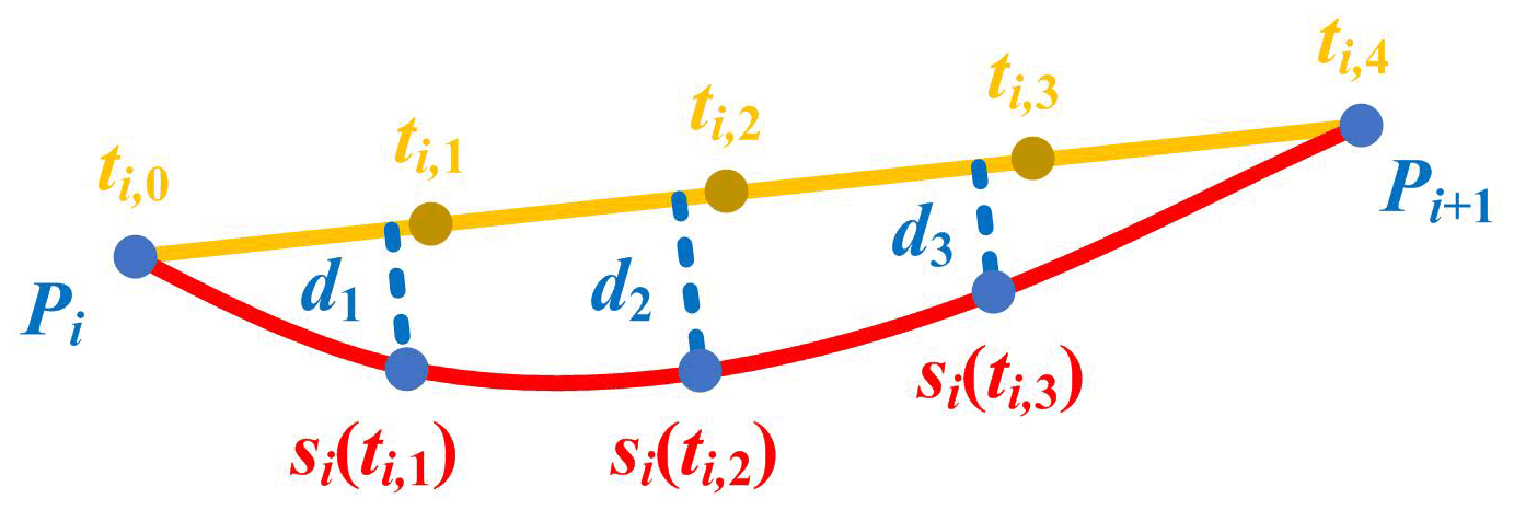
• Step 1. For the ith trajectory segment P_iP_i+1, as shown in Fig. 3, let $t_{i,\mathrm{0}}=\mathrm{0}$, $t_{i,\mathrm{4}}=T_i$ and the maximum contour error ${\mathit{\epsilon }}_{i,m}=\mathrm{0}$.

• Step 2. Set the times $t_{i,\mathrm{1}}=(t_{i,\mathrm{4}}-t_{i,\mathrm{0}})/\mathrm{4}$, $t_{i,\mathrm{2}}=\mathrm{2}(t_{i,\mathrm{4}}-t_{i,\mathrm{0}})/\mathrm{4}$, and $t_{i,\mathrm{3}}=\mathrm{3}(t_{i,\mathrm{4}}-t_{i,\mathrm{0}})/\mathrm{4}$. Calculate the corresponding position points s_i(t_i,1), s_i(t_i,2), and s_i(t_i,3) for each indicated time from Eq. (2) with the calculated trajectory parameters. Then compute the distances d₁, d₂, and d₃ to the line segment P_iP_i+1 (Fig. 3).

• Step 3. Set ${\mathit{\epsilon }}_{i,m}=max(d_{\mathrm{1}}$, d₂, d₃). If ${\mathit{\epsilon }}_{i,m}>\mathit{\epsilon }$, the maximum contour error of the ith segment curve s_i(t_i) exceeds the prescribed threshold and the motion period T_i is reduced in proportion to the amount that the contour error threshold has been exceeded as

  $$\begin{array}{}\text{(27)}& T_i=T_i-{\displaystyle \frac{\left|{\mathit{\epsilon }}_m-\mathit{\epsilon }\right|}{{\mathit{\epsilon }}_m}}{\displaystyle \frac{T_i}{\mathrm{2}}}.\end{array}$$

  And let $f_i=\mathrm{1}/\left(\mathrm{4}{T}_i\right)$; otherwise, contour error threshold has been met in the ith segment of the trajectory.

• Step 4. For all synthesized trajectory segments, go through the above steps to control their contour errors. If contour error threshold has been exceeded in any segment, go to the Sect. 2.2.4 and recalculate trajectory parameters with the updated segment trajectory periods and fundamental frequencies.

Figure 3 Contour error of the ith segment.

3 Simulation validations

In this section, simulations demonstrating the effectiveness and performance of the proposed low-harmonic trajectory synthesis algorithm are presented. The results are also compared with those obtained with one of the commonly used polynomial algorithms for synthesizing robot trajectories. Visual Studio 2013 was used to implement both algorithms, and results are plotted in MATLAB 2015.

To evaluate the proposed algorithm, a quintic polynomial algorithm (Perumalsamy et al., 2019), which interpolates data points using quintic polynomials with continuous displacement, velocity, acceleration, and jerk values, is used as the comparison algorithm.

As shown in Fig. 4, a letter Z-shaped pattern is selected as the path, which contains five data points, P₁(0,3), P₂(3,3), P₃(1.5,1.5), P₄(0,0), P₅(3,0), and consists of four segments, P₁P₂, P₂P₃, P₃P₄, P₄P₅. The following variables were initialized: a fundamental frequency of f=20 Hz, the motion periods of segments, T₁=0.68 s, T₂=0.32 s, T₃=0.32 s, T₄=0.68 s, and a contour error limit of ε=0.25 mm. The synthesized trajectories synthesized by applying the two algorithms are shown in Fig. 4, and we can see that they are all smooth.

Figure 4 Letter Z-shaped path and synthesized trajectories.

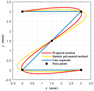
Figure 5 shows that both algorithms can obtain smooth axis displacement, velocity, and acceleration profiles, and the jerk of the proposed algorithm is also smooth because of satisfying continuous jounce conditions, while that of the comparison algorithm is not smooth.

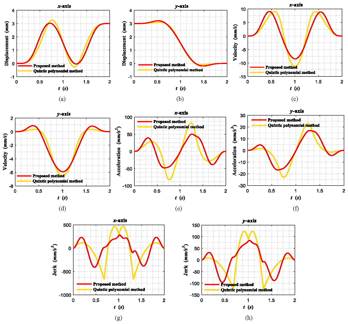
Figure 5 Comparison of kinematic profiles: (a) x-axis displacement profiles, (b) y-axis displacement profiles, (c) x-axis velocity profiles, (d) y-axis velocity profiles, (e) x-axis acceleration profiles, (f) y-axis acceleration profiles, (g) x-axis jerk profiles, and (h) y-axis jerk profiles.

To evaluate the proposed algorithm further, frequency spectrum distribution of the synthesized kinematic profiles is studied using Fourier integration. In the plots of Fig. 6, the axial displacements, velocities, accelerations, and jerks of the trajectory synthesized using the quintic polynomial algorithm are shown to contain a considerable number of high-harmonic components. As a result, the related actuators are required to produce high-frequency components, which for high-speed motions would in general be beyond their dynamic response and could excite natural modes of vibration of the system. As expected, the velocity, acceleration, and jerk profiles of the synthesized trajectory with the proposed algorithm are seen in Fig. 6 to only contain a finite number of low-harmonic components.

Figure 6 Comparison of the Fourier analysis: (a) x-axis displacement profiles, (b) y-axis displacement profiles, (c) x-axis velocity profiles, (d) y-axis velocity profiles, (e) x-axis acceleration profiles, (f) y-axis acceleration profiles, (g) x-axis jerk profiles, and (h) y-axis jerk profiles.

To explain how trajectories with high-harmonic components affect vibration of machinery, an undamped, 1-degree-of-freedom linear spring–mass system of Fig. 7 is used to model the vibration behavior of a machine. Let the spring have a spring rate and free length of k and l, respectively, and the mass of the system be m. The displacements of the mass and the system from their initial position are u and d, respectively. From the Newton's second law, the system equation of motion is seen to be

$$\begin{array}{}\text{(28)}& m\ddot{u}=-k(u-d-l).\end{array}$$

Let $z=u-d-l,\ddot{z}=\ddot{u}-\ddot{d}$, and set the natural frequency of the spring–mass system to be

$$\begin{array}{}\text{(29)}& f_n={\displaystyle \frac{\mathrm{1}}{\mathrm{2}\mathit{\pi }}}\sqrt{{\displaystyle \frac{k}{m}}}=\mathrm{27}\mathrm{Hz}.\end{array}$$

Then, Eq. (28) can be rewritten as

$$\begin{array}{}\text{(30)}& \ddot{z}=-{\left(\mathrm{2}\mathit{\pi }{f}_n\right)}^{\mathrm{2}}z-\ddot{d}.\end{array}$$

Figure 7 Spring–mass system.

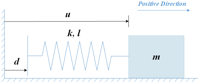
Now, take the x-axis motion profiles calculated using the aforementioned two algorithms as input to the dynamic system described by Eq. (30). The input motion $\ddot{d}$ is the x-axis acceleration profile, i.e., $\ddot{d}=a_x\left(t\right)$. Substituting $\ddot{d}=a_x\left(t\right)$ into Eq. (30) and solving the resulting second-order ordinary differential equation, the vibrational motion of the mass m of the spring–mass system of Fig. 7 is determined.

As can be seen in Fig. 8, the displacement z of the proposed algorithm is smoother than that of the quintic polynomial algorithm. In addition, when the x-axis motion ends, the mass m comes to a stop with the proposed algorithm, while the mass of the quintic polynomial algorithm continues to vibrate with its natural mode. It is noted that the trajectories synthesized using the quintic polynomial algorithm contain a significant number of high-harmonic content, which would in general cause excitation of the system modes of vibration irrespective of their frequencies. The synthesized trajectories of the proposed algorithm, however, only contain a finite number of low-frequency harmonics in its velocity, acceleration, and jerk terms and even in their higher-order derivatives, which would minimize the number of high-harmonic components in the required actuation forces/torques. The fundamental frequency of the trajectory pattern can also be selected to avoid natural modes of vibration of the system. As a result, the system should be capable of operating with minimal vibration.

Figure 8 Vibrations of the mass–spring system of Fig. 6: (a) quintic polynomial algorithm, (b) proposed algorithm.

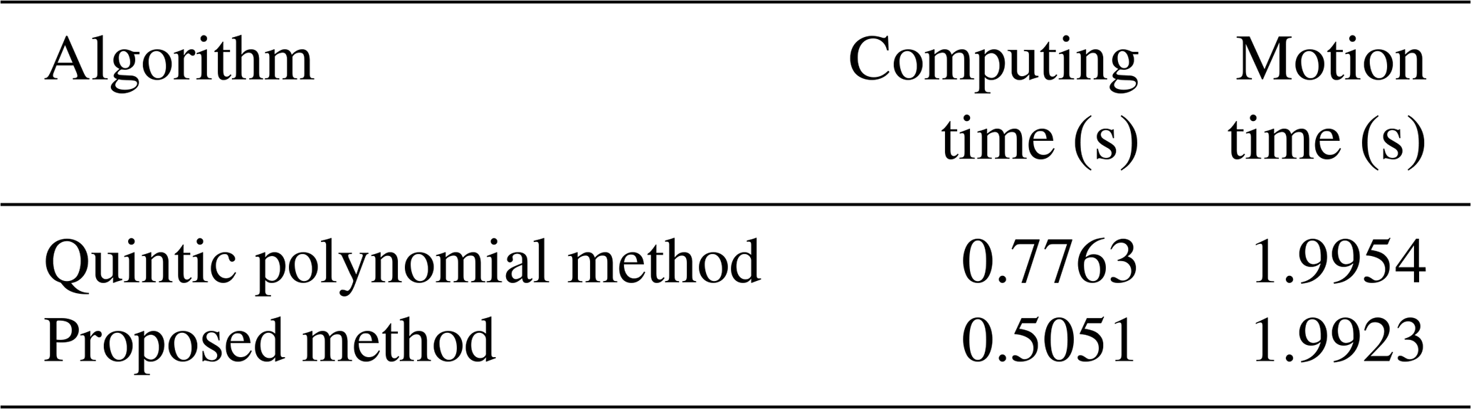
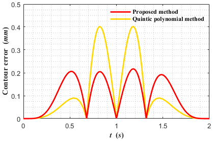
Table 1 shows that the motion times of both algorithms are almost same and that the computing time cost by the proposed algorithm (0.5051 s) is shorter than the quintic polynomial algorithm (0.7763 s). The contour errors with both algorithms are presented in Fig. 9. As can be seen, the maximum contour error of the quintic polynomial algorithm is also significantly larger than that of the proposed algorithm.

Table 1 Comparison of computing and motion times.

Figure 9 Contour errors.

4 Conclusions

A trajectory pattern method (TPM)-based method and related algorithm has been developed for synthesis of low-harmonic trajectories for high-speed and high-precision machinery. The trajectory synthesis with the TPM is performed with a prescribed fundamental frequency and continuous jounce boundary condition, which would minimize the number of high-harmonic components in the required actuation forces/torques and avoid excitation of the system modes of vibration.

The developed TPM-based algorithm is shown to yield smooth axial kinematic profiles with low-harmonic content and thereby reduces demand on the dynamic response of the drive actuators. As a result, and with the capability of selecting the frequency of the fundamental harmonic of the synthesized trajectory and its harmonics present in the actuating forces/torques, a machine can operate at high speed and high precision.

In comparison with the previously published algorithms, the developed algorithm has the following advantages:

• i.

  The trajectories are constructed with a sinusoidal function with a selected fundamental frequency, which can avoid excitation of the natural modes of vibration of the machinery system.

• ii.

  All segment displacement, velocity, acceleration, and jerk profiles are expressed by a sinusoidal time function consisting of a selected frequency fundamental harmonic and at least its first three harmonics, and the overall synthesized trajectories only contain a finite number of low harmonics, which minimizes the number of high-frequency harmonics of the required actuation forces/torques with the aforementioned operational advantages.

• iii.

  The developed algorithm can realize smooth axial kinematic control action with specified contour error limitation.

In the provided example, since the trajectory synthesis with the TPM is performed with a prescribed fundamental frequency and continuous jounce boundary condition, the trajectory pattern must include at least three harmonics of the fundamental frequency. More harmonics may, however, be used to provide more trajectory parameters to achieve, for example, higher precision, usually at the expense of operating speed.

In the provided example, a point-to-point trajectory was shown to be synthesized. The method and algorithm may readily be used to synthesize general trajectories with or without defined intermediate precision points or with more loosely defined precision points to, for example, minimize contour errors.