the Creative Commons Attribution 4.0 License.
the Creative Commons Attribution 4.0 License.
 | 20 May 2021
Programming piston displacements for constant flow rate piston pumps with trigonometric transition functions
Zhongxu Tian
An analytical method for programming piston displacements for constant flow rate piston pumps is presented. A total of two trigonometric transition functions are introduced to express the piston velocities during the transition processes, which can guarantee both constant flow rates and the continuity of piston accelerations. A kind of displacement function of pistons, for two-piston pumps, and two other kinds, for three-piston pumps, are presented, and the physical meaning of their parameters is also discussed. The results show that, with the given transition functions, cam profiles can be designed analytically with parameterized forms, and the maximum accelerations of the pistons are determined by the width of the transition domain and the rotational velocities of the cams, which will affect contact forces between cams and followers.
- Article
(1822 KB) - Full-text XML
- BibTeX
- EndNote


The piston pump is a type of positive displacement pump in which the high-pressure seal reciprocates with the piston, which is a vital component in hydraulic fluid power systems. There are four types of displacement pumps commonly used in the industry, i.e. gear pumps, vane pumps, radial piston pumps, the axial piston pumps (Ye et al., 2019). Piston pumps are widely used in many fields, such as oil exploitation, hydraulic circuits, and control systems, owing to their high specific power, efficiency, and reliability. However, piston pumps also have some shortcomings when compared to when compared to equivalent pumps.
Piston pumps usually contain several cylinders. Multiphase pumps can efficiently increase oil and gas production in crude oil drilling owing to their good internal compression and anti-gas resistance performance (Deng et al., 2018; Dogru et al., 2004; Falcimaigne and Decarre, 2008; Hua et al., 2011). However, oscillations in the pump flow rate may give rise to pressure pulsations which can lead to vibrations, noise, and harmful impacts on pipelines (Karassik et al., 2001). Therefore, the flow rate of the piston pump must be kept constant. The invariability in the pump flow rate is also essential for controlling systems, and one can obtain the desired control only through adjusting the rotational speed of the pump cams. Pre-pressure airbags and infusion pumps are generally used to fulfil the constant flow rate requirement. Still, there are some patents aiming at solving this problem (Couillard and Garnier, 1998; Sipin, 2002). They provide the methods and apparatus for supplying constant liquids. The system, according to the invention, comprises several primary pumping units in parallel on a single mixing head. By adjusting the phases, the piston strokes, and their velocities, each piston output flows intermittently in order to obtain a substantially constant discharge rate. Furthermore, a novel variable displacement pump architecture (Foss et al., 2017) was designed for displacement control circuits that uses the concept of alternating flow (AF) between piston pairs that share a common cylinder. The AF pump was constructed from two inline triplex pumps, which is efficient across a wide operating range. Wilhelm and Van De Ven (2014a) presented the optimization and machine design of an 8.5 kW, high-pressure, variable displacement, triplex prototype. The pump can be applied to a wide range of applications with little compromise, compared with present variable displacement pumps. These scholars have improved the structure of the piston pumps to obtain a more stable flow rate. However, if the suitable combination of the velocity of multiple piston pumps can be achieved, the total flow rate can be kept constant.

To make the piston pump adapt to the developmental needs of the modern industrial sector, high efficiency and energy saving, small flow, and pressure pulsation are the goals of piston pump design (Gandhi et al., 2014; Huang et al., 2017; Wilhelm and Van De Ven, 2014b). Initially, most of the piston pumps were driven by the crank-connecting rod mechanism. Its remarkable feature was the transient flow rate, which caused a pressure pulsation in the discharge and suction system and had a direct impact on the working effect (Berezovskii and Nakorneeva, 1969). Therefore, the low shear, constant flow, non-fluctuating piston pump with a cam transmission mechanism as the power solved the problem of flow and pressure fluctuations. Dong et al. (2002) compared and analysed the performances of the crank-connecting rod piston pump and the cam piston pump. In the end, they pointed out that, under the same conditions, the cam-driven piston pump had a smaller flow pulsation and inertial load, which was conducive to extending the service life. Therefore, in this paper, the pistons are driven by rotational cams to pump liquid out in turns. The structural diagram of the piston pump is shown in Fig. 1. The piston pumps contain three cylinders driven by cam systems with a flat-faced follower.
By changing the speed of the drive motor to adjust the flow, it is necessary to add a corresponding control and detection system, which increases the design difficulty and the design cost. Therefore, the improvement of the cam profile is a fundamental improvement. With the development of technology, the cam profile has been deeply studied, which makes the cam system drive more flexible, and it has less impact vibration (Gatti and Mundo, 2010; Hsieh, 2010). The proposed piston pump motion law determines the shape of the cam profile curve. In turn, the cam profile surface parameters affect the motion and dynamic characteristics of the plunger and even the whole machine. The cam profile includes the transition section and the working section. The transition section can eliminate the impact of the pressure pulsations of the piston pump, and the working section directly affects the work efficiency of the piston pump (Li et al., 2013). To this end, we must first determine the movement law of the follower, namely the plunger.
The simplest way to keep constant flow rates is to give proper design schemes of piston displacements that are finally determined by the profiles of cams. Traditionally, the design of cams was based on the desired movement function by specifying translated displacements of the follower in terms of a cam rotational angle φ, and the movement is usually expressed analytically. During the process of designing cam profiles, the designer is often confronted with many problems, such as the satisfaction of the specific displacement, velocity, and acceleration constraints. Also, the continuity of the displacement curve, at least through the second derivative, becomes necessary, especially for high-speed cams. The cam profile synthesis method, using spline functions, was well used in the design of cam profiles because of its superior controllability (Nguyen and Kim, 2007; Tsay and Huey, 1993; Yoon and Rao, 1993). However, when the higher order of the derivative for a displacement curve is required continuously, the order and term number in the spline curves increase and more coefficients of the terms have to be determined, which causes the amount of calculation to be much larger (Zhou et al., 2016). When the inertia force and load change according to the harmonic curve, it only corresponds to a few harmonic frequencies, while the polynomial corresponds to more frequencies, making it difficult to plan frequency and avoid resonance (Di et al., 2006; Tian and Chen, 2006). To achieve the goal of continuity in piston movements, trigonometric splines (Choubey and Ojha, 2007; Neamtu et al., 1998) are usually employed in the design of various cam mechanisms.
In the existing literature, the acceleration of this kind of cam was not continuous, and the transition function was difficult to use when planning frequency and avoiding resonance. Moreover, these researchers are devoted to optimizing the structure of piston pumps and lack a systematic method for the design of piston pumps driven by the cam mechanism. Therefore, this paper presents the study on an innovative design method for high-speed cams using trigonometric transition function, selects the basis and law of intermediate parameter, and discusses the physical meaning of their parameters.
In order to meet the constant flow rates of the pumps and C1 property of their piston velocities, this paper is devoted to the study of the design method of proper cams to meet both of these two conditions at the same time. Furthermore, a kind of displacement function of pistons, for two-piston pumps, and two other kinds, for three-piston pumps, are also presented analytically. The main structure of this paper is as follows: in Sect. 1, the research status and the drawbacks of previous studies are summarized. In Sect. 2, the transition functions are defined. In Sect. 3, cams for two-piston pumps are designed. In Sect. 4, the design parameters of two-piston pumps, including the flow rate and the maximum accelerations, are reported. In Sect. 5, one type of piston velocity, driven by cam A for three-piston pumps, is presented, and for which the method is similar to two-piston pumps. In Sect. 6, two types of piston velocities are applied to cam B. In each subdomain, one piston is designated in the backward stroke, and the other two are designated in the forward stroke. In Sect. 7, the cam profiles are computed by rational theories. In Sect. 8, the conclusions are given.
For piston pumps with a constant flow rate and a good performance, the piston velocities should meet the requirements of constant flow rates and C1 continuity in the whole movement cycles.
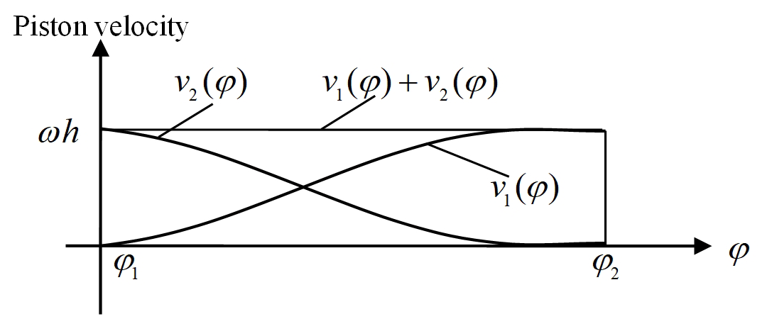
The velocities of the forward and backward strokes, corresponding with the output and input processes of the cylinder, have to be changed between the two processes in some transition domains. Suppose that when one piston moves forward with a speed-up velocity v1(φ) from 0 to ωh in an angular domain [φ1,φ2], there should be another piston moving forward with a speed-down velocity v2(φ) from ωh to 0 in the same domain to provide a constant flow rate of the pump, and the two velocities should satisfy the following (shown in Fig. 2):
where ω is the constant angular velocity of the cams driving the pistons, and h is a constant to be determined by the desired flow rate of pumps.
According to the C1 properties of the velocities, v1(φ) and v2(φ) should be smooth and meet the following:
In order to simplify the task, a couple of standard transition functions, f1(θ) and f2(θ), are searched in the standard domain [0,π] to express the velocities in the following forms:
According to conditions (1) and (2), f1(θ) and f2(θ) should satisfy the following requirements.
-
Transition function f1(θ) should be C1 in [0,π] and satisfy the following:
-
In order to meet condition (1), f2(θ) should satisfy the following:
and the following boundary conditions:
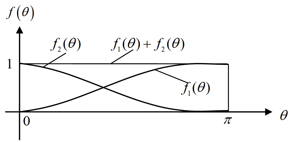
In Fig. 3, f1(θ) and f2(θ) are similar to cosine or sine functions; therefore, f1(θ) is supposed to take the following trigonometric form:
Using boundary conditions (4) and (5), unknown parameters b and c are determined, and Eq. (9) becomes the following:
According to boundary condition (6), f2(θ) should take the following form:
Obviously, f2(θ) meets boundary conditions (7) and (8). At last, the velocities in the transition domain [φ1,φ2] can be expressed in the following forms:
The acceleration of the piston is another important factor for piston pumps, which affects the contact forces between cams and the followers. According to Eq. (12), the accelerations in the transition domain are as follows:
Ignoring the directions, the maximum accelerations are [φ1,φ2] are as follows:
From Eq. (14), we can see that the maximum accelerations in the transition domain are determined by angular velocities of the cam, the width of the transition domain, and h, which should be included in the designation of the pumps.
It should be noted that spline functions might be workable, but they are more complex and could cause more difficulties in the computation of displacement functions.
By lending the previous transition functions to the design of cam profiles, the goal of achieving the constant flow rate and the continuity of piston displacement through the second derivative can be achieved easily.
For a two-piston pump, the phase between the two pistons is usually 180∘. Figure 3 shows a simple velocity curve for the two-piston pump. The liquid is pumped out alternately, and the flow rate remains constant.
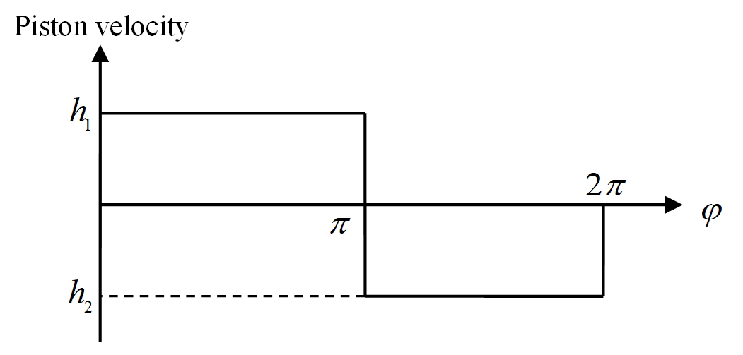
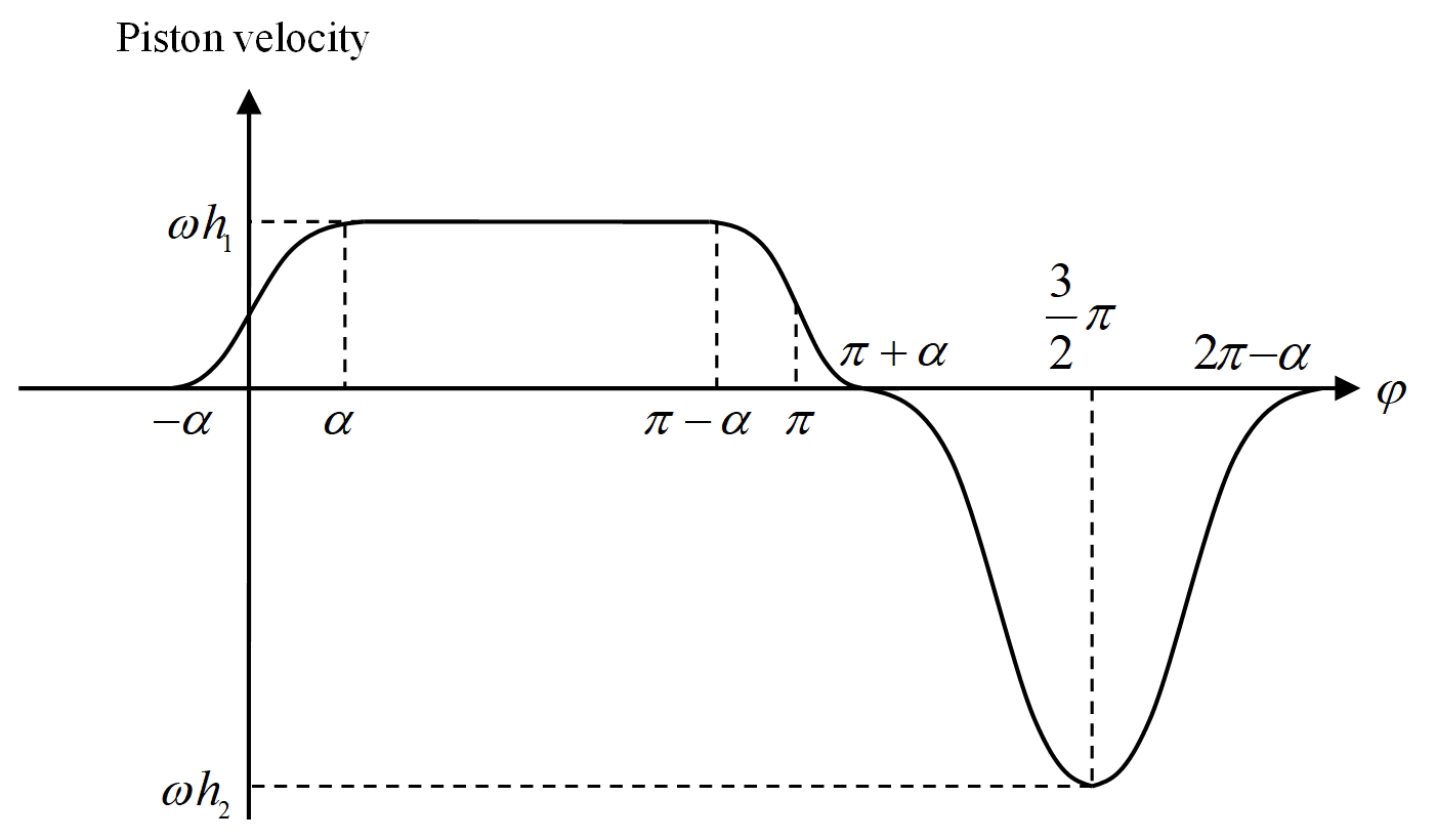
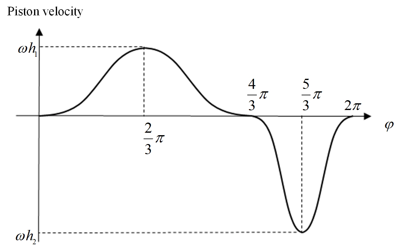
However, the velocity is not continuous, as shown in Fig. 4. Given the fact that the acceleration goes to infinity sometimes, serious collisions between cams and pistons will occur. Therefore, transition processes are needed to guarantee the C1 property of the velocities and the C0 property of the accelerations. By introducing the transition functions defined in Sect. 2, the piston velocity v(φ) can be expressed with piecewise functions in the following forms (see Fig. 5):
where φ denotes the cam rotational angle, h1 and h2 are constants determining the maximum velocity of the pistons in the forward stroke and the backward stroke, and α is the half-width of the transition domain.
The velocity of the pistons in the backward stroke is not constant since it has no effect on the constant flow rates, and it can obtain the minimum acceleration, so contact forces are also reduced. It easy to verify that the velocity function, given by Eq. (15), is C1, and the acceleration is continuous.
For a two-piston pump, Eq. (15) describes the velocity of piston 1. The same function applies to the velocity of piston 2, provided (φ+π) is substituted for φ. Thus, for the interval , piston 1 and 2 have velocities given, respectively, by the first and the third expression in Eq.. (15), and their sum is ωh1. For the interval , the second expression in Eq. (15) gives the velocity of piston 1, while piston 2 is executing a backward stroke and not delivering any flow. Therefore, the total flow rate is again given by ωh1.
The displacement function s(φ) can be obtained, as follows, by integrating the velocity (Eq. 15) over time:
where C1, C2, C3, C4, and C5 are constants. As the displacement is continuous, we should have the following:
Therefore, C2, C3, C4, C5, and h2 can be expressed in the following forms with h1 and C1:
The velocity v(φ) and height s(φ) can be determined after h1 and C1 are given appropriate values.
When the cams run with the angular velocity ω, and the velocity of the pistons is ωh1, then the flow rate per minute of the pump is as follows:
where r denotes the number of revolutions per minute, and S is the cross-sectional area of the cylinders.
From Eq. (16), the minimum and maximum displacements of the pistons can be obtained as follows:
For knife-edge and flat-faced follower systems, smin is the base circle radius of the cam. For the roller follower system, the base circle radius is smaller than smin, and the difference is the follower radius. Similar results are also obtained for three-piston pumps, as discussed in Sect. 7.
The stroke of the pistons H, which is the difference between the maximum and the minimum heights, is as follows:
According to Eqs. (20) and (21), C1 determines the size of the cam.
From Eq. (15), the accelerations of pistons are derived in the following form:
Therefore, the maximum accelerations in the forward and backward strokes, and , are as follows:
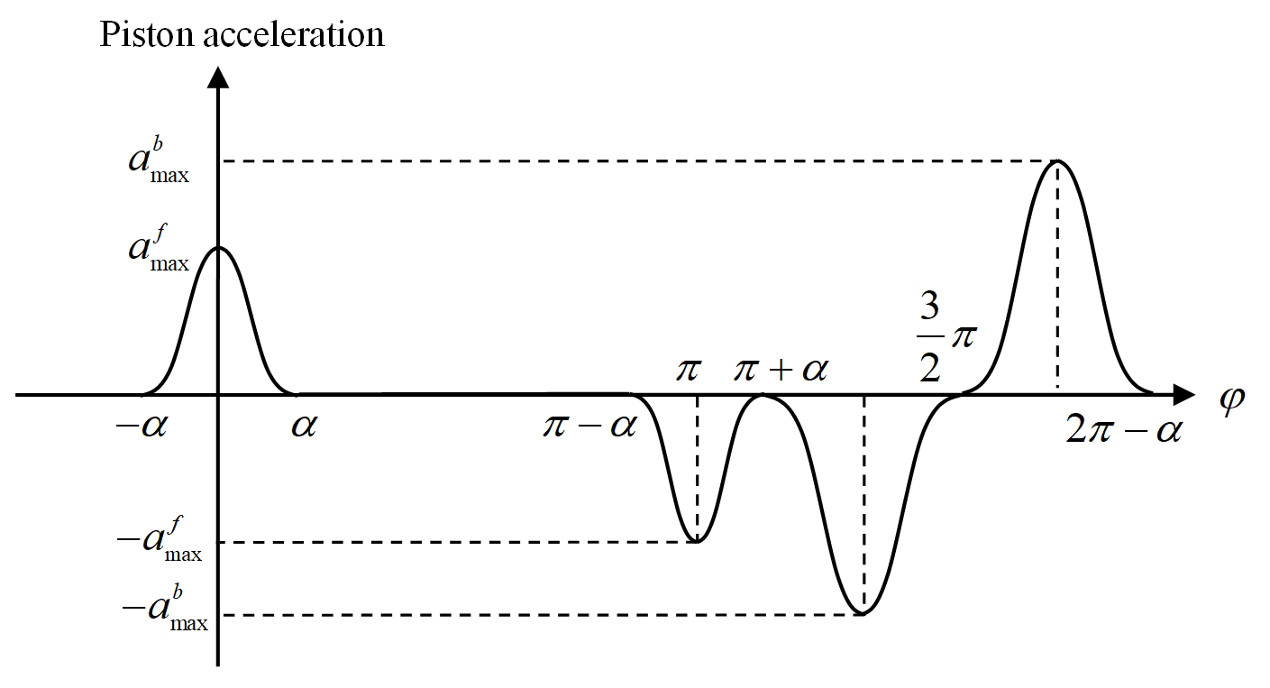
In Eq. (25), the relationship between h1 and h2 (Eq. 18), is used. Figure 6 shows the acceleration curve in one cycle. The maximum accelerations of the pistons in every forward stroke come twice, and one is positive and the other negative. The procedure is similar for the backward stroke.
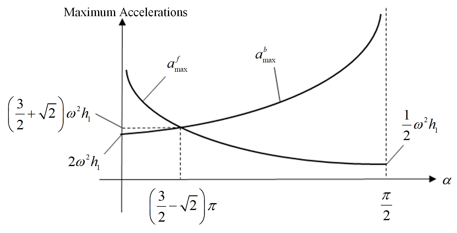
Figure 7Piston maximum accelerations respect to transition angles (α) of the two-piston pump.
Figure 7 shows the maximum accelerations corresponding to different transition angles α. It can be seen that the maximum accelerations in the forward stroke decrease as the angle α increases and that the maximum accelerations in the backward stroke increase at the same time. Synthetically, α can be determined according to practical applications.
The three-piston pumps are used in many places, such as polymer injection in the exploitation of oil and control systems. In general, the difference in phase among the three pistons is 120∘, and two types of piston velocities, driven by cam A and cam B, are presented in this and the next section.
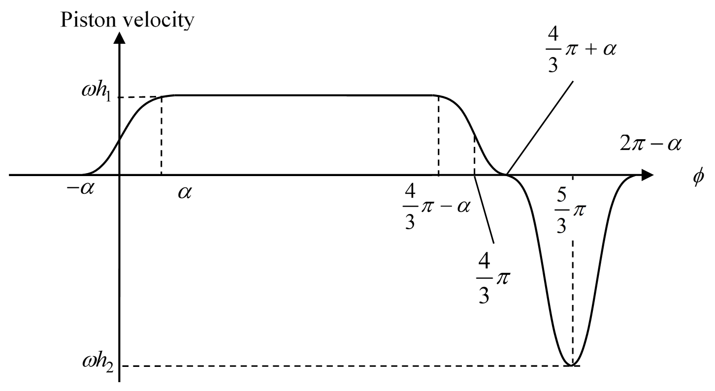
Using a similar method to that of two-piston pumps, the piston velocity v(φ), using cam A, is chosen in the forms shown in Fig. 8, and consists of five piecewise functions expressed with the following formula:
where h1 and h2 are constants determining the maximum velocities in forward and backward strokes, and α is a half-width of the transition domain.
For a three-piston pump, Eq. (26) gives the velocity of piston 1. The same equations apply to the velocity of piston 2 and piston 3, provided () and () are substituted for φ, respectively. Thus, for the interval , pistons 1, 2, and 3 have velocities given, respectively, by the first, second, and third expressions in Eq. (26), and their sum is 2ωh1. For the interval , the second expression in Eq. (26) gives the velocity of piston 1 and 2, while piston 3 is executing the backward stroke and not delivering any flow. Therefore, the total flow rate is again given by 2ωh1.
Thus, the flow rate of the three-piston pump is constant, and the flow rate per minute has the following form:
where r denotes the number of revolutions per minute of the cam, and S is the cross-sectional area of the cylinders.
By integrating the velocity Eq. (26) over time, we can obtain the following displacement function:
where C1, C2, C3, C4, and C5 are constant parameters.
By means of the following continuity conditions:
C2, C3, C4, C5, and h2 can be determined as follows:
As s4(φ) and s5(φ) share the same form, Eq. (28) can be rewritten as follows:
After the values of h1 and C1 are chosen, the displacement curve of the cams can be determined. The physical meaning of h1 and C1 is the same as that of the two-piston pumps presented in Sect. 3.
According to Eq. (31), the minimum and maximum displacements of the pistons are as follows:
and the stroke of the pistons H is as follows:
Similarly, the acceleration is as follows:
and the maximum accelerations in the forward and backward strokes, and , are as follows:
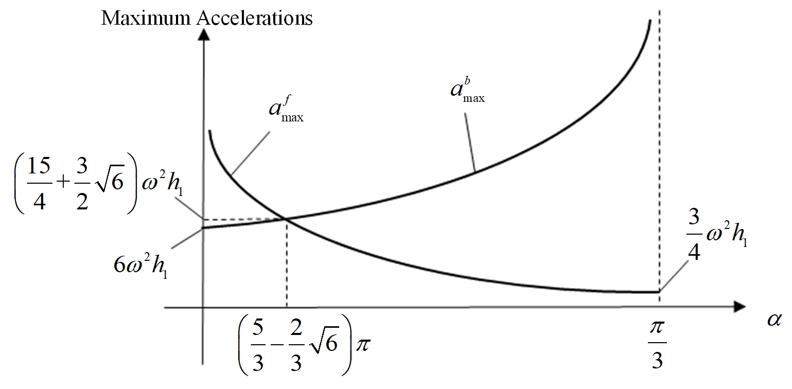
Figure 9 shows the accelerations corresponding to different transition angles α. It can be seen that the maximum accelerations in the forward stroke decrease as α increases, and that the maximum accelerations in the backward stroke increase simultaneously.
For two-piston pumps, one piston must be in the forward stroke with constant velocity to provide a constant flow rate when the other piston is in the backward stroke. For three-piston pumps, there can be two pistons in the forward stroke to provide the total constant flow rate when the third piston is in the backward stroke. Thus, each cycle can be divided into three 120∘ subdomains. In each subdomain, one piston is designed to be in the backward stroke, and the other two are designed to be in the forward stroke to achieve the total constant flow rate. The velocity v(φ), specified by cam B, can be designed in the form illustrated in Fig. 10 and expressed with the following piecewise functions:
where h1 and h2 are constants determining the maximum piston velocity in the forward and backward strokes.
According to Eqs. (9) and (11), f1(t) and f2(t) satisfy the following:
Therefore, Eq. (38) can be rewritten as follows:
For a three-piston pump, Eq. (40) gives the velocity of piston 1. The same equations apply to the velocity of piston 2 and piston 3, provided () and () are substituted for φ, respectively. Thus, for interval , piston 1 and 2 have velocities given, respectively, by the first expression in Eq. (40), while piston 3 is executing a backward stroke and not delivering any flow. Therefore, the total flow rate is given by ωh1. Similar results will be drawn for intervals and . Therefore, the flow rate of the pump is constant, which can be put as follows:
where r denotes the revolutions of the cam per minute, and S is the cross-sectional area of the cylinders.
By integrating the velocity function over time, the displacement curve s(φ) can be obtained in the following forms:
where C1 and C2 are the constants of the integrations.
Since the cam profiles are continuous, the height function must obey the following:
From Eq. (43), we have the following:
At last, Eq. (42) can be rewritten as follows:
Noting Eq. (42), the minimum and maximum displacements of the pistons are as follows:
and the stroke of the pistons, H, is as follows:
Similarly, the acceleration is as follows:
and the maximum accelerations in the forward and backward strokes, and , are as follows:
As it provides a greater width of transition domains than cam A in both the forward and backward processes, cam B can run with lower accelerations of pistons, which can also be seen through the comparison among Eqs. (34), (35), (48), and (49).
The displacements corresponding to the cams are designed in the previous sections, and the cam profiles corresponding to different followers can be determined by rational theories (Casciola and Morigi, 1996; González-Palacios and Angeles, 2012; Jensen, 2020). The computational formulas of the cam profiles corresponding to these followers are given in the following.
The cam profiles corresponding to knife-edge followers can be prescribed by the following functions:
where the displacement function, s(φ), is described by Eqs. (11), (20), (28), and (32).
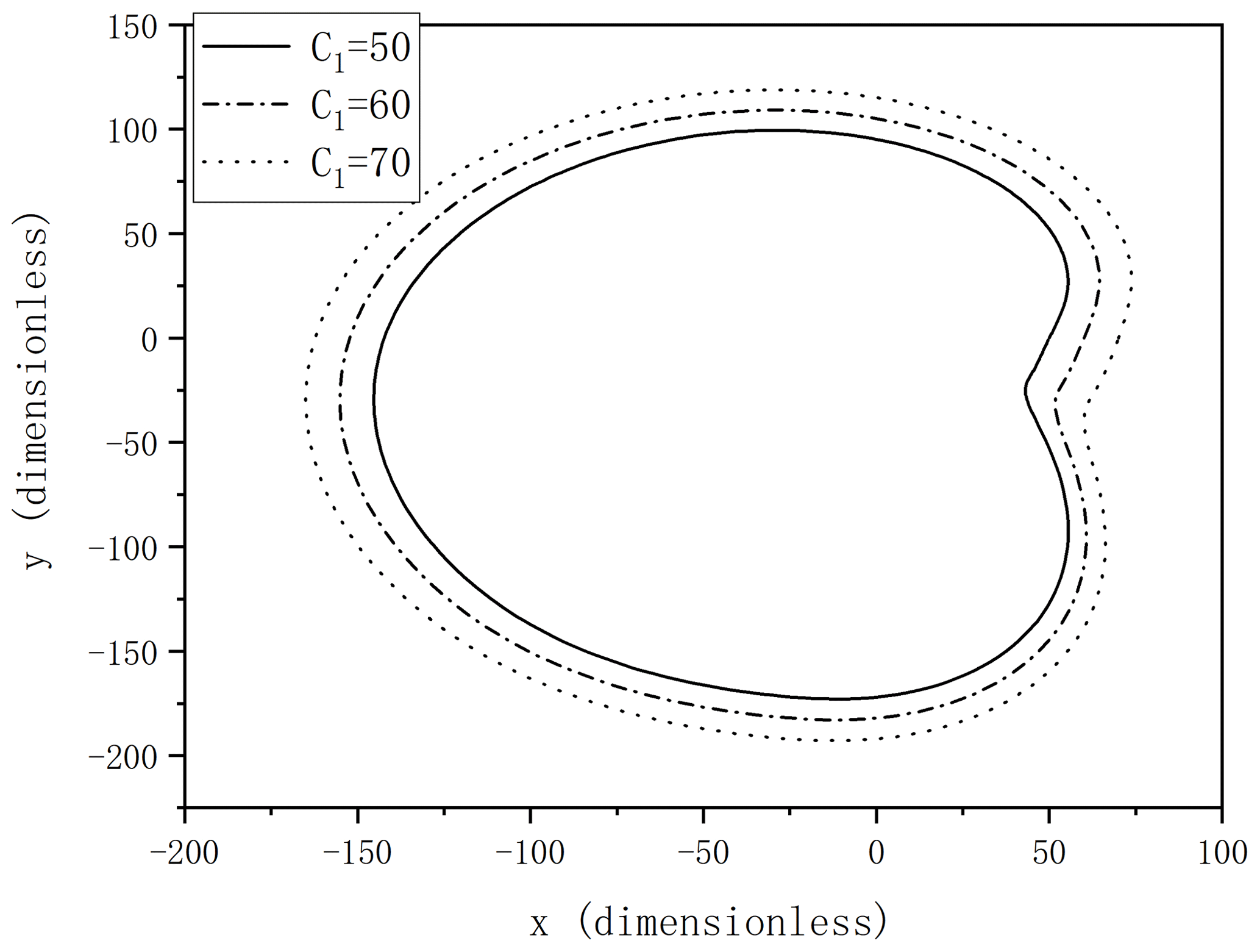
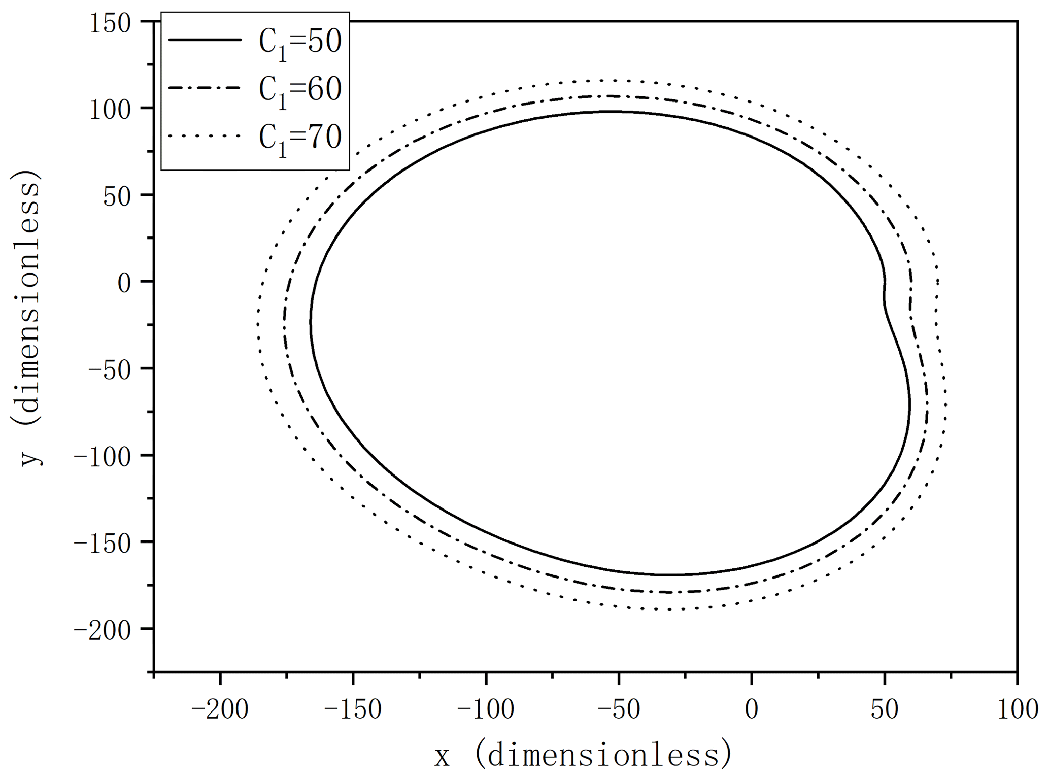
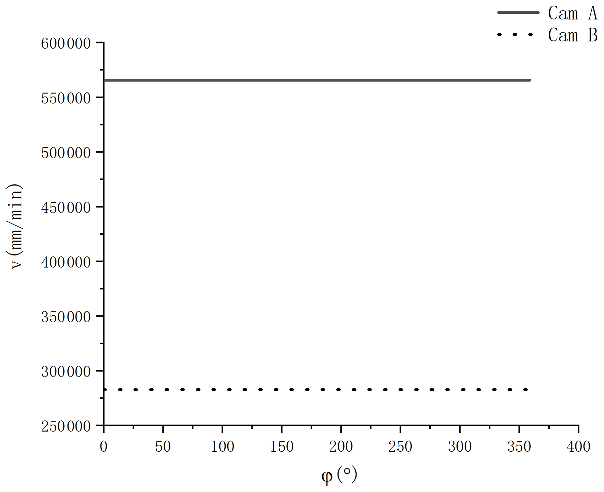
Take the cams driven by hydraulic fluid power systems as a specific calculation example. According to the flow rate and the application requirements, the system parameters were fixed as h1 = 30 mm, α = 10∘, and the sizes of the cam C1 are, respectively, 50, 60, and 70 mm. The contour shapes of cam A and cam B are obtained as shown in Figs. 11 and 12. When the cams ran with an angular velocity, the cross-sectional area of the cylinders were fixed as r = 1500 r min−1, S = 100π mm2, and π = 3.1416, leading to the velocities of the piston pumps in cam A and cam B shown in Fig. 13. The velocities of the piston pumps are both kept constant, and the values are, respectively, 565 488 and 282 744 mm min−1. Therefore, the flow rates per minute of the piston pumps are, respectively, QA = 177.65 L min−1 and QB = 88.83 L min−1.
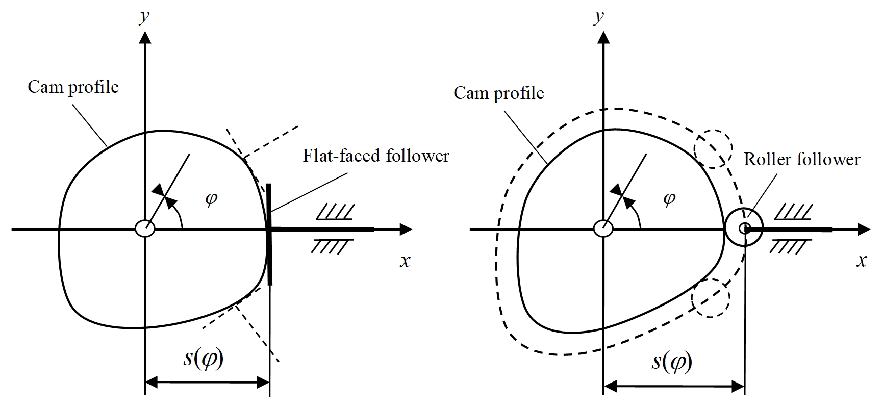
Flat-faced and roller followers have usually been used in high-speed cams rather than knife-edge followers because of the rapid rate of wear. Flat-faced followers can only work with the cam profile of all external curves with a small pressure angle, high efficiency, and good lubrication. The roller followers improved the contact condition between the follower and the cam profile, which can greatly reduce frictional losses and bear a high load.
Flat-faced followers (Fig. 14) are the most common in piston pumps, and the cam profiles, described by the coordinates x and y, can be given with the following formulae:
Corresponding to the roller followers (Fig. 14), the cam profile, coordinating with X and Y, can be expressed by the following formulae:
where rr denotes the radius of the roller, and (x,y) corresponds to the cam profile with knife-edge follower given by Eq. (52).
Trigonometric splines are employed in the design of various cam mechanisms as transition functions, which can to help to plan the frequency and avoid resonance. With the given transition functions, cam profiles, required to provide a constant flow rate, can be designed analytically with parameterized forms, and the parameters can be determined according to application requirements. The piston acceleration continuity can also be guaranteed simultaneously.
Defined in a standard domain, the transition functions are uniformly described, with very simple forms, and can be used conveniently by lending coordinate transformations.
Two types of piston velocities among the three pistons and two types of cam systems with different followers are presented to provide more choices for the design of the piston pumps.
The maximum accelerations of the pistons are determined by the width of the transition domain and the rotational velocities of the cams, which will affect contact forces between cams and followers. The two parameters should be noted during the designation of the cams.
| φ | Cam rotational angle |
| C1 | Property of piston velocities |
| C0 | Property of the accelerations |
| ω | Constant angular velocity of cam |
| h | A constant |
| v(φ) | Piston velocity |
| α | Half-width of the transition domain |
| f(θ) | Standard transition function |
| s(φ) | Piston displacement |
| a(φ) | Piston accelerations |
| Q | Flow rate |
| r | Number of revolutions per minute |
| S | Cross-sectional area of the cylinders |
| Maximum accelerations in the forward strokes | |
| Maximum accelerations in the backward strokes | |
| H | Stroke of the piston |
All codes generated or used during the study are available from the corresponding author upon request.
All data sets used in the paper can be requested from the corresponding author.
All work related to this paper has been accomplished by the efforts of both authors. ZT proposed the design of the piston pumps, analysed the numerical results, and wrote the paper. XL provided guidance on theoretical methods, edited the paper, and prepared the figures.
The authors declare that they have no conflict of interest.
Zhongxu Tian and Xingxing Lin greatly acknowledge the financial support from the National Key Research and Development Program of China and the Shanghai Engineering Research Center of Marine Renewable Energy, which made this research possible.
This research has been supported by the National Basic Research Program of China (973 Program; grant no. 2019YFD0900800) and the Shanghai Engineering Research Center of Marine Renewable Energy (grant no. 19DZ2254800).
This paper was edited by Daniel Condurache and reviewed by three anonymous referees.
Berezovskii, L. and Nakorneeva, T.: Failure characteristics of cranks of piston type circulating pumps and high pressure compressors, Chem. Petrol. Eng+., 5, 805–809, https://doi.org/10.1007/bf01153179, 1969.
Casciola, G. and Morigi, S.: Modelling of curves and surfaces in polar and Cartesian coordinates, Dept. of Math., Bologna, Italy, 21 pp., 1996.
Choubey, N. and Ojha, A.: Constrained curve drawing using trigonometric splines having shape parameters, Comput. Aided Design, 39, 1058–1064, https://doi.org/10.1016/j.cad.2007.06.005, 2007.
Couillard, F. and Garnier, D.: Piston pumping system delivering fluids with a substantially constant flow rate, Office, Patent No. 5755561, 1998.
Deng, H. Y., Liu, Y., Li, P., Ma, Y., and Zhang, S. C.: Integrated probabilistic modeling method for transient opening height prediction of check valves in oil-gas multiphase pumps, Adv. Eng. Softw., 118, 18–26, https://doi.org/10.1016/j.advengsoft.2018.01.003, 2018.
Di, Y., Tian, Z. X., and Ma, L.: Designing Cam Profile Curves of Constant Flow Pump Based on Analytical Method in Chinese, Machine Tool & Hydraulics, 10, 83–85, https://doi.org/10.3969/j.issn.1001-3881.2006.10.027, 2006.
Dogru, A. H., Hamoud, A. A., and Barlow, S. G.: Multiphase pump recovers more oil in a mature carbonate reservoir, J. Petrol. Technol., 56, 64–67, https://doi.org/10.2118/83910-Jpt, 2004.
Dong, H. R., Zhang, H. F., and Pei, J. F.: The correlation analyses of the performances between the cam-drive mechanism reciprocating pump and the crack-connecting rod reciprocating pump, Journal of Jiangsu Institute of Petrochemical Technology, 14, 10–13, https://doi.org/10.3969/j.issn.2095-0411.2002.04.004, 2002 (in Chinese).
Falcimaigne, J. and Decarre, S.: Multiphase production: pipeline transport, pumping and metering, Editions Technip, Paris, 2008.
Foss, R. J., Li, M., Barth, E. J., Stelson, K. A., and Van de Ven, J. D.: Experimental Studies of a Novel Alternating Flow (AF) Hydraulic Pump, in: ASME/BATH 2017 Symposium on Fluid Power and Motion Control, Sarasota, Forida, USA, 2017, https://doi.org/10.1115/fpmc2017-4315, 2017.
Gandhi, V. C. S., Kumaravelan, R., Ramesh, S., Kumar, K. N., and Chinnaiah, S.: Design and analysis of quad-acting reciprocating pump: A novel approach, International Journal for Engineering Modelling, 27, 125–130, 2014.
Gatti, G. and Mundo, D.: On the direct control of follower vibrations in cam-follower mechanisms, Mech. Mach. Theory, 45, 23–35, https://doi.org/10.1016/j.mechmachtheory.2009.07.010, 2010.
González-Palacios, M. A. and Angeles, J.: Cam synthesis, Springer Science & Business Media, Berlin, 2012.
Hsieh, J. F.: Design and analysis of cams with three circular-arc profiles, Mech. Mach. Theory, 45, 955–965, https://doi.org/10.1016/j.mechmachtheory.2010.02.001, 2010.
Hua, G., Falcone, G., Teodoriu, C., and Morrison, G.: Comparison of Multiphase Pumping Technologies for Subsea and Downhole Applications, Oil Gas Facilities, 1, 36–46, https://doi.org/10.2118/146784-MS, 2011.
Huang, Y. Q., Nie, S. L., Ji, H., and Nie, S.: Development and Optimization of a Linear-Motor-Driven Water Hydraulic Piston Pump, T. Can. Soc. Mech. Eng., 41, 227–248, https://doi.org/10.1139/tcsme-2017-1016, 2017.
Jensen, P. W.: Cam design and manufacture, CRC Press, New York, 2020.
Karassik, I. J., Messina, J. P., Cooper, P., and Heald, C. C.: Pump Handbook, McGraw-Hill Education, New York, 2001.
Li, Y., Yang, J., and Li, K.: Analysis and Optimization of High-speed Gasoline Engine Cam Profile, Appl. Mech. Mater., 278–280, 184–188, https://doi.org/10.4028/www.scientific.net/AMM.278-280.184, 2013.
Neamtu, M., Pottmann, H., and Schumaker, L. L.: Designing NURBS cam profiles using trigonometric splines, J. Mech. Design, 120, 175–180, https://doi.org/10.1115/1.2826956, 1998.
Nguyen, V. T. and Kim, D. J.: Flexible cam profile synthesis method using smoothing spline curves, Mech. Mach. Theory, 42, 825–838, https://doi.org/10.1016/j.mechmachtheory.2006.07.005, 2007.
Sipin, A. J.: Continuous fluid injection pump, Office, Patent No. 6368080, 2002.
Tian, Z. X. and Chen, X. C.: The Designation of Cam's Contour for Piston Pump with Steady Flux, in: IFIP International Federation for Information Processing, Springer, Boston, MA, 231–236, https://doi.org/10.1007/0-387-34403-9_31, 2006.
Tsay, D. M. and Huey, C. O., Jr.: Application of Rational B-Splines to the Synthesis of Cam-Follower Motion Programs, J. Mech. Design, 115, 621–626, https://doi.org/10.1115/1.2919235, 1993.
Wilhelm, S. R. and Van De Ven, J. D.: Design of a Variable Displacement Triplex Pump, in: International Fluid Power Exposition, Las Vegas, NV, 2014a.
Wilhelm, S. R. and Van De Ven, J. D.: Efficiency Testing of an Adjustable Linkage Triplex Pump, V001T001A037, in: ASME/BATH 2014 Symposium on Fluid Power and Motion Control, Bath, United Kingdom, https://doi.org/10.1115/fpmc2014-7856, 2014b.
Ye, S., Zhang, J. H., Xu, B., Zhu, S. Q., Xiang, J. W., and Tang, H. S.: Theoretical investigation of the contributions of the excitation forces to the vibration of an axial piston pump, Mech. Syst. Signal Pr., 129, 201–217, https://doi.org/10.1016/j.ymssp.2019.04.032, 2019.
Yoon, K. and Rao, S. S.: Cam Motion Synthesis Using Cubic Splines, J. Mech. Design, 115, 441–446, https://doi.org/10.1115/1.2919209, 1993.
Zhou, C., Hu, B., Chen, S., and Ma, L.: Design and analysis of high-speed cam mechanism using Fourier series, Mech. Mach. Theory, 104, 118–129, https://doi.org/10.1016/j.mechmachtheory.2016.05.009, 2016.
- Abstract
- Introduction
- Transition functions
- Design of cams for two-piston pumps
- Design parameters of two-piston pumps
- Design of cam A for three-piston pumps
- Design of cam B for three-piston pumps
- Computation of cam profiles
- Conclusions
- Appendix A: Nomenclature
- Code availability
- Data availability
- Author contributions
- Competing interests
- Acknowledgements
- Financial support
- Review statement
- References