the Creative Commons Attribution 4.0 License.
the Creative Commons Attribution 4.0 License.
 | 18 May 2021
Center-point steering analysis of tracked omni-vehicles based on skid conditions
Yunan Zhang
Yinghui Shang
Tao Huang
Mengfei Yan
Existing center-point steering models of a tracked omni-vehicle seldom consider the skid of the track (roller) grounding section, which is inconsistent with the actual steering process. In this study, for the three typical layout types, rectangular, hybrid, and centripetal, the steady center-point steering motion of a tracked omni-vehicle under skid conditions is analyzed and a correction model is investigated. The numerical solution of the absolute lateral offset of the steering pole is obtained, and the influences of various structural parameters on the numerical solution are discussed. The steering angular velocity reduction coefficient is calculated, and the angular velocity of vehicles is corrected. The simulation of center-point steering motion is carried out on eight virtual prototypes, and the center-point steering motion experiment is carried out on three physical prototypes. The results show that the established correction model is more in line with the steering reality of the tracked omni-vehicle, and it can play a role in correcting the center-point steering angular velocity.
- Article
(6478 KB) - Full-text XML
- BibTeX
- EndNote


An omnidirectional mobile robot (vehicle) system can move in any direction for the 3 degrees of freedom on a plane, and it can also rotate at any angle with zero radius in situ, with flexible movement and convenient control. It has unparalleled advantages in narrow areas requiring high speed and high mobility (Wang, 2018). With the exception of robots containing running mechanisms similar to universal wheels (caster wheels) (Cao, 2018; Clavien et al., 2018; Yang et al., 2018) and robots in the form of a single ball (Karavaev and Kilin, 2017; Madhushani et al., 2017), omnidirectional mobile robots are divided into wheeled and tracked omni-robots according to different running mechanisms.
The running mechanisms that constitute wheeled omni-robots (hereinafter referred to as the “wheeled omni-mechanisms”) mainly include the Mecanum wheel (Wang, 2018), alternate wheel (Park et al., 2016), MY wheel (Tong, 2017), and spherical omnidirectional wheel (Tadakuma et al., 2008, 2009). Poor load capacity, high requirements for flatness and cleanliness of the walking environment, and poor off-road and obstacle crossing performance are the common shortcomings of wheeled omni-robots. One of the improvement measures is to develop tracked omni-robots.
The running mechanisms of tracked omni-robots (hereinafter referred to as the “tracked omni-mechanisms”) mainly include the free-roller track (Chen et al., 2002), Vuton crawler (Roh et al., 2013), Mecanum wheel crawler (Mortensen Ernits et al., 2017; Guan and Yuan, 2019), omnidirectional mobile track (Zhang, 2017; Li et al., 2012; Xing et al., 2018; Ma et al., 2015), planar omnidirectional crawler mobile mechanism (Tadakuma et al., 2017; Takane et al., 2019; Yu et al., 2020), omni-crawler (Tadakuma et al., 2012, 2014), and other omnidirectional tracks. According to whether it has the ability of active movement in two non-collinear directions, the tracked omni-mechanism can be divided into two types: active tracked and semi-active tracked omni-mechanisms. An active tracked omni-mechanism has problems such as a complex structure and poor load capacity. The semi-active tracked omni-mechanism has strong load capacity and a wide range of applications, and it is suitable for small robots (Roh et al., 2013; Zhang and Yang, 2018) and large machinery (Mortensen Ernits et al., 2017; Fang et al., 2020). From the perspective of the projection of the grounding section of the running mechanism, an omnidirectional mobile track is the more representative of a semi-active tracked omni-mechanism. The research on vehicles using the omnidirectional mobile track (hereinafter referred to as a “tracked omni-vehicles”) is more mature (Zhang and Yang, 2018; Zhang and Huang, 2015).
The center-point steering motion is one of the important motion forms of a tracked omni-robot. The center-point steering theory of a traditional tracked vehicle (such as the tank) cannot be directly applied to a tracked omni-robot. For a tracked omni-vehicle with a rectangular layout, Huang et al. (2014) analyzed the velocity relationship between the base point on the track grounding section and the maximum slip point during the steering process and obtained the relationship between the maximum steering slip ratio and the structural parameters of the vehicle. Huang et al. (2014) lacked analysis of other points on the track except the maximum slip point. The maximum steering slip ratio cannot represent all the characteristics of the center-point steering motion of the vehicle. For a tracked omni-vehicle with a rectangular layout, Zhang et al. (2015) analyzed the velocity relationship between the center point of the grounding section of a single track and other points during the turning process and obtained the expression of the average slip velocity of the grounding section of a single track. Zhang et al. (2015) lacked an analysis of the track layout and did not consider the impact of the track slip on the steering angular velocity of the vehicle. For a tracked omni-vehicle with hybrid layout, Yang et al. (2019b) analyzed the influence of the roller offset angle on steering motion from the perspective of steering torque. Yang et al. (2019b) lacked design parameter analysis other than the roller offset angle, and lacked the analysis of the center-point steering motion of the whole vehicle.
A theoretical analysis of center-point steering motion should be carried out for a variety of typical layout tracked omni-vehicle, and a correction model should be established. The research object should be all the points of the track grounding section while focusing on the analysis of the motion relationship between the track grounding section and the vehicle. The correction model can correct the angular velocity and time of the vehicle, as well as give the relationship between the design parameters such as the roller offset angle and the steering performance. This allows the designer to evaluate the steering performance of the vehicle during the design stage and then optimize the design.
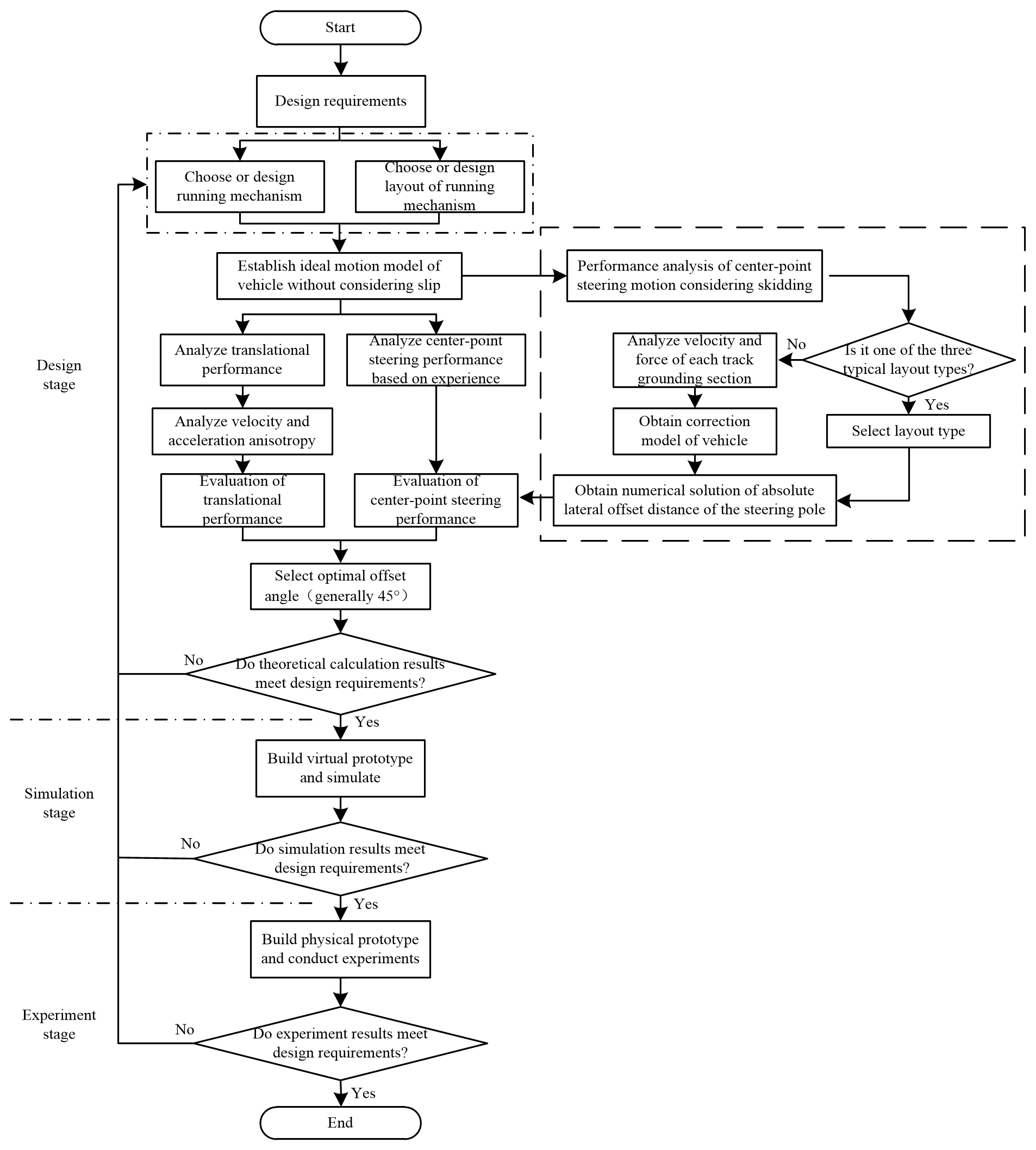
The current design process of the tracked omni-vehicle, as shown in Fig. 1, is divided into three steps.
-
Select or design the preliminarily structure and layout of the mobile mechanism according to the design requirements.
-
Establish a motion model of the vehicle. Because the slip in translational motion can be ignored, the performance and anisotropy of translational motion are analyzed based on the ideal motion model. Because the slip in the center-point steering motion cannot be ignored, the performance of the center-point steering motion cannot be analyzed based on the ideal motion model, and the performance can only be analyzed based on experience. Based on the results of the analysis, the performance of the vehicle's translational and center-point steering motion is evaluated. Through the evaluation results, the optimal value of the roller offset angle (generally 45∘) is obtained.
-
Compare the theoretical results with the design requirements to see if the design requirements are met.
Analyzing the performance of the center-point steering motion of the vehicle based on experience introduces uncertainty. The performance of the center-point steering motion of the vehicle should be analyzed according to the content in the dashed box in Fig. 1. If the layout of the vehicle to be designed belongs to one of the three types studied in this paper, then the theoretical model given in this article will be directly applied. If not, we should first analyze the velocity and force of the track grounding section and then obtain the correction model of the vehicle. According to the correction model, the numerical solution of absolute lateral offset distance of the steering pole is obtained. The center-point steering motion performance of the vehicle is evaluated according to the numerical solution.
Based on an omnidirectional mobile track, in this study, the center-point steering motion of the three typical types of tracked omni-vehicles, with rectangular, hybrid, and centripetal layouts, is analyzed and the mathematical model is established. Eight virtual prototypes are established in ADAMS, and the center-point steering motion simulation is performed. Three physical prototypes are established, and center-point steering experiments are performed. The simulation and experimental data are analyzed and compared with the theoretical model. The research results of this study can provide guidance for the structural design of the semi-active tracked omni-mechanism represented by the omnidirectional mobile track and a vehicle with this mechanism, and the results can provide a basis for analysis and evaluation. The research results of this study can also provide a reference for the research of an active tracked omni-mechanism and a vehicle with this mechanism and other tracked omni-robots.
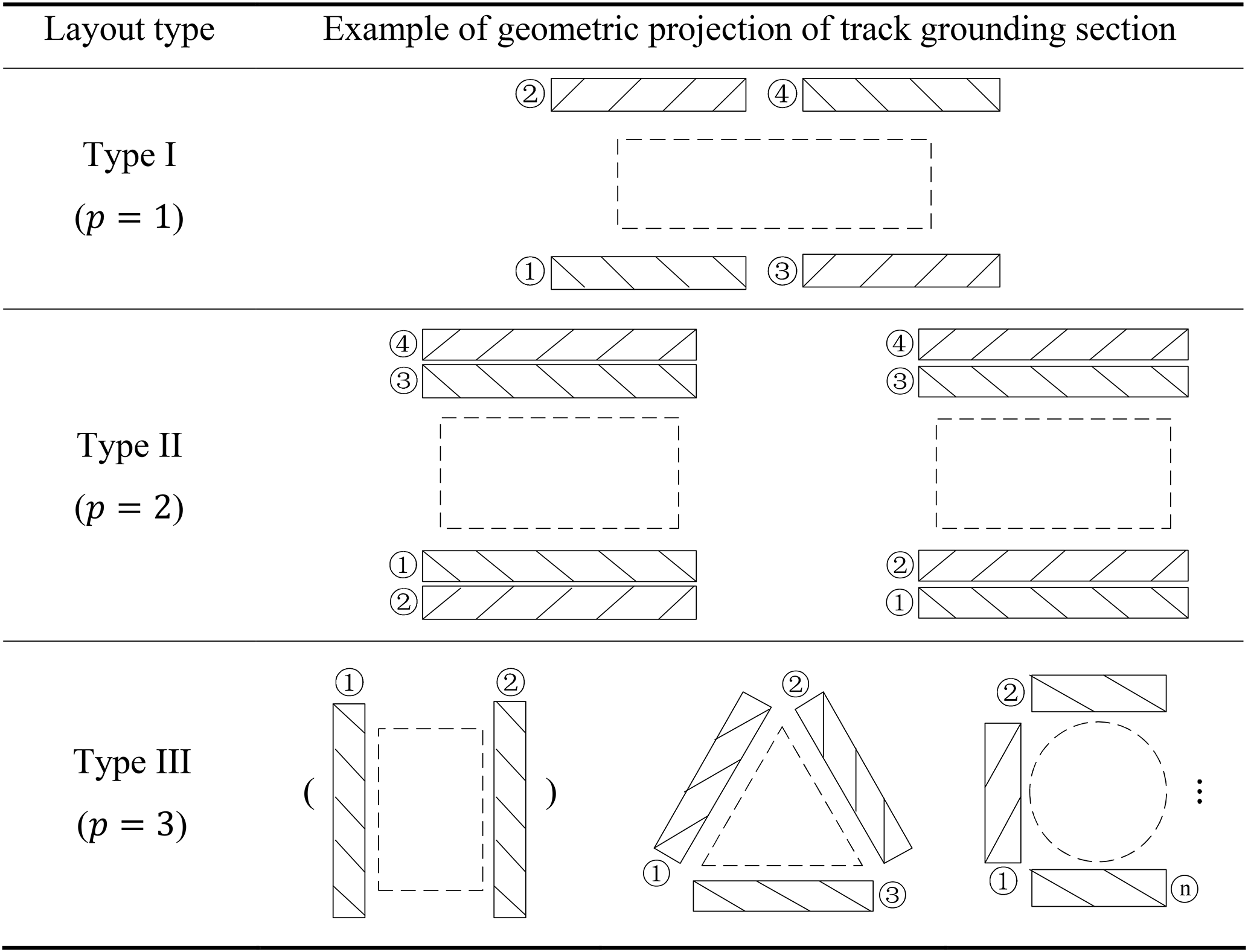
The typical layout types of tracked omni-vehicles and other tracked omni-robots are mainly rectangular (Mortensen Ernits et al., 2017; Zhang and Yang, 2018; Zhang and Huang, 2015; Zhang et al., 2015; Huang et al., 2014; Singh et al., 2017; Hua and Zhang, 2019; denoted Type I), hybrid (Yang et al., 2019a, b; Liu et al., 2018; denoted Type II), and centripetal layouts (Chen et al., 2002; Roh et al., 2013; Y. Zhang et al., 2017, 2019; Zhang, 2018; X. Zhang et al., 2016; denoted Type III). A schematic of the layout of the three types of tracked omni-vehicles is shown in Table 1, where p represents the types, with (refer to Appendix A for the meaning of all of the symbols in this article). The tracks are numbered in Table 1. The solid rectangle represents the geometric projection of the track grounding section, the short oblique line represents the axis of the ground roller, and the dotted line represents the vehicle body. The Type III vehicle with two tracks can complete the center-point steering motion but cannot complete the omnidirectional motion, so it is not an omni-vehicle and it is distinguished by brackets in Table 1.
According to the ideal inverse kinematics equation of the tracked omni-vehicle given in Zhang and Huang (2015) without considering the slip, the ideal inverse kinematics equations of the three types shown in Table 1 can be obtained as shown in Eq. (1), wherein the subscript i represents the number i track of the vehicle, . The applicable condition of Eq. (1) is that the track has a shorter landing length (Zhang and Huang, 2015):
where
In the formula, , vxp is the translational velocity along the x axis and vyp is the translational velocity along the y axis. ωzp is the angular velocity of the theoretical center-point steering motion without considering slippage (hereinafter referred to as “ideal center-point steering motion”). ωpi is the speed of the driving sprocket, rpi the radius of the pitch circle of the driving sprocket, and αpi the offset angle of the roller, . βpi is the angle between the center of the track and the center of the vehicle, and lpi is the distance between the center of the track and center of the vehicle. θpi is the angle between the coordinate system of the track and the coordinate system of the vehicle. The necessary condition for the vehicle to achieve omnidirectional motion is that the velocity inverse Jacobian matrix of the system is full rank (Wang, 2018), i.e., rank(Jωp)=3. It should be pointed out that Eq. (1) is also the ideal inverse kinematics equation of the omni-platform composed of Mecanum wheels. This means that the essence of Eq. (1) is to equate the omnidirectional mobile track to the Mecanum wheel located in the center of the track, that is, ignoring all grounding points except the center point of the track.
Letting Lpi be the length of the track grounding section, generally, the radius of each driving sprocket of the same vehicle is the same and the grounding length of each track is the same, i.e., rpi=rp1 and Lpi=Lp1. If only the center-point steering motion is studied, the rotation speed of all driving sprockets in a vehicle can be set to be the same, i.e., ωpi=ωp1.
The Type I vehicle consists of four tracks, which are located at the four corners of the vehicle body. Tracks (1) and (2) are symmetrical along the longitudinal axis of the vehicle body, tracks (3) and (4) are symmetrical along the longitudinal axis of the vehicle body, tracks (1) and (3) are symmetrical along the transverse axis of the vehicle body, and tracks (2) and (4) are symmetrical along the transverse axis of the vehicle body. Tracks (1) and (4) have the same roller offset angle, and tracks (2) and (3) have the same roller offset angle. The signs of the roller offset angles of tracks (1) and (4) are opposite to those of tracks (2) and (3). For a Type I vehicle, in Eq. (1), l1i=l11, , , , , , , and , where . Setting Bypi=|lpisin βpi| and Bxpi=|lpicos βpi|, By1i=By11, Bx1i=Bx11.
A Type II vehicle consists of four tracks, with two tracks arranged on each side of the vehicle body, and the roller offset angles of the same side track are opposite. For a Type II vehicle, in Eq. (1), l21=l23, l22=l24, , , , , , , By2i=0, Bx21=Bx23, and Bx22=Bx24.
A Type III vehicle consists of several tracks that are evenly distributed around the geometric center of the vehicle body, and the roller offset angles of each track are equal. For a Type III vehicle, in Eq. (1), l3i=l31, , and α3i=λ3.
In summary, the ideal center-point steering model (kinematic equations) of the three types of vehicles can be obtained from Eq. (1) as shown in Eq. (2):
To establish a motion correction model based on skid conditions (hereinafter referred to as the “correction model”) for the smooth steering of a tracked omni-vehicle on a horizontal road surface, the following assumptions are made (Cheng et al., 2006, 2007).
-
The vehicle is symmetrical about its longitudinal and transverse planes, and the center of mass and the geometric center of the vehicle coincide.
-
The ground pressure of the track (roller) is uniformly distributed, regardless of the pressure changes of the roller when it approaches the ground and when it leaves the ground.
-
The vehicle has low-speed uniform steering, ignoring the influences of the centrifugal force and angular velocity changes.
-
The track is a uniform and flexible belt, regardless of the width and misalignment of the track.
-
The driving resistance coefficient of the vehicle does not change due to steering.
The following is an analysis of the center-point steering motion for Type I, II, and III vehicles.
3.1 Analysis of center-point steering motion of Type I vehicle
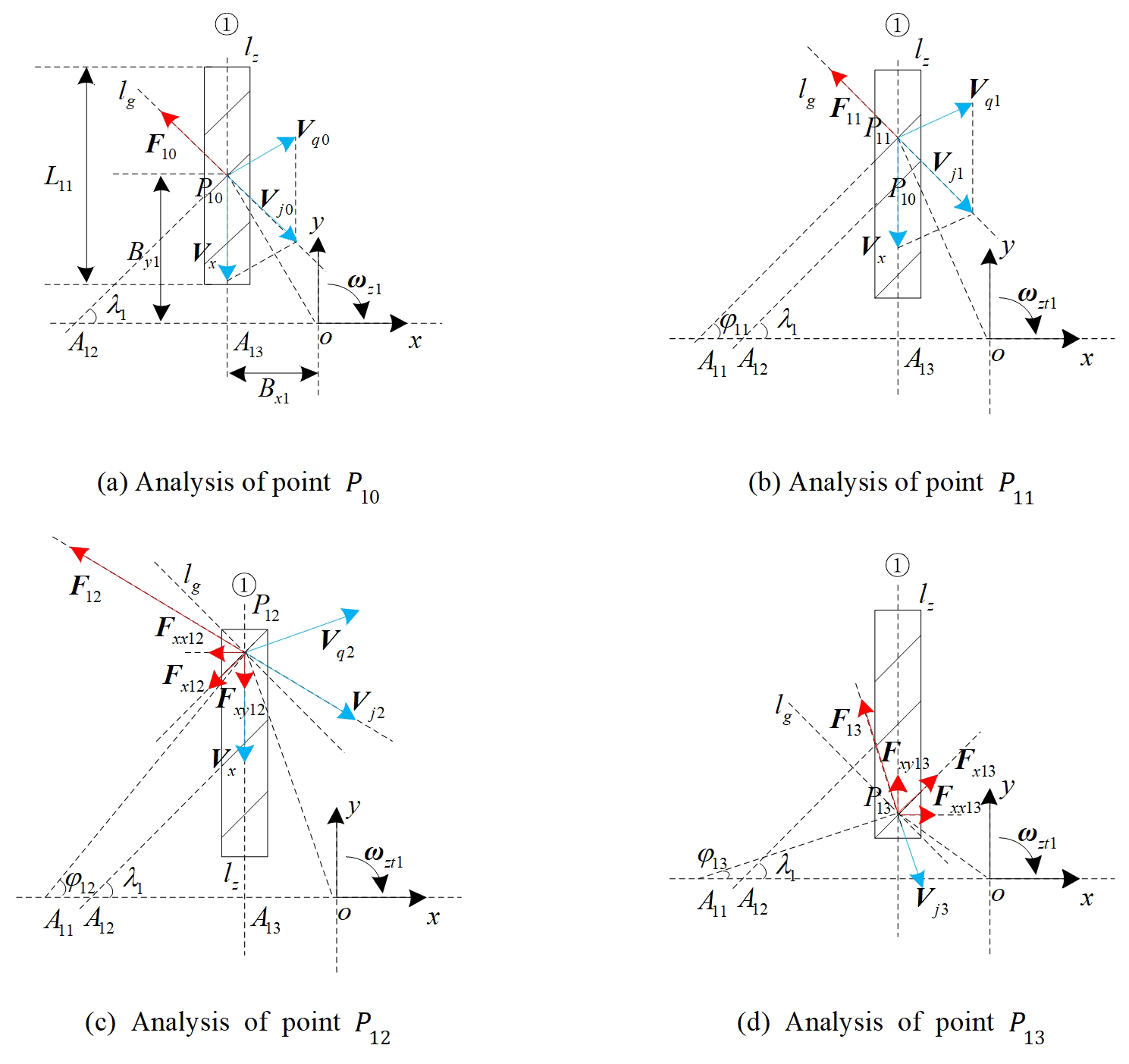
Taking track (1) of the Type I vehicle as an example, the point on the longitudinal symmetry axis of the track grounding section is selected and the center-point steering motion in four parts, as shown in Fig. 2a–d, is analyzed. The vehicle has a clockwise center-point steering motion, with clockwise as the positive direction. In Fig. 2a–d, the blue arrow represents the velocity vector, and the red arrow represents the force vector. The parameters, such as the amplitude and angle of each vector in Fig. 2, are slightly exaggerated for the convenience of presentation and do not represent the actual values. Taking the horizontal ground as the Earth absolute coordinate system XOY, a follow-up coordinate system xoy is established on the vehicle body, where point o is the plane projection of the geometric center of the vehicle. lz is the straight line where the longitudinal symmetry axis of the track grounding section lies. Ppk is the type k grounding point between the rollers on track (1) of the p-type vehicle and the ground, and . Pp0 is the grounding point in the ideal center-point steering motion. Pp1, Pp2, and Pp3 are the grounding points in the center-point steering motion considering the slip. Pp1 is the grounding point at which the degree of slippage is zero, Pp2 the grounding point with an ordinate greater than Pp1, and Pp3 the grounding point with an ordinate smaller than Pp1.
3.1.1 Analysis of ideal center-point steering motion
First, the ideal center-point steering motion, as shown in Fig. 2a, is analyzed. Point P10(−Bx11By11) is the geometric center of the ground plane of track (1). lg is the straight line in the free rotation direction of the grounded roller, and it is the vertical line of the roller axis. A13 is the intersection of lz and the ox axis. The extension line of the roller axis direction passing point P10 and the straight line where the ox axis is located intersect at point A12. Vx is the relative velocity vector of the track, and the direction is along the negative direction of the y axis. Vqk is the following velocity vector, which is perpendicular to the oPk vector. Vjk is the absolute velocity vector, which is perpendicular to the A11P1k vector. Due to the interaction between the ground and the grounded roller, a reverse force F1k vector is generated in the opposite direction of its absolute speed. Letting , where μ is the steering resistance coefficient (Song et al., 2008, 2009), mp the mass of the p-type velocity, and g the acceleration of gravity, it is noted that Mpk and Tpk are the steering resistance torque and the driving torque, respectively, of the k-type grounding point of track (1) of the p-type vehicle.
According to the derivation process (Zhang and Huang, 2015) of Eq. (1), it can be seen that Eq. (1) is only applicable to the geometric center point of the plane of the track grounding section, as shown in point P10 in Fig. 2a. At this time, Vj0 and lg are collinear, while F10 and Vj0 are collinear and opposite in direction. Because Vj0 is in the free-rotation direction of the roller, no slippage occurs. At this time, the effect of F10 on the roller is only the free rotation of the roller. Therefore, A12 is the instantaneous turning center of the grounding section of track (1) without considering the slip.
In the ideal center-point steering motion, the instantaneous turning center of the left-hand track grounding section of a traditional dual-track longitudinally symmetrical tracked vehicle represented by a tank (hereinafter referred to as the “traditional tracked vehicle”) is point A13. The comparison shows that the steering pole of the Type I vehicle has an original lateral offset from A13 to A12 under ideal circumstances.
3.1.2 Analysis of point at which slip is zero
The movement of point P11(−Bx11y0) shown in Fig. 2b is now analyzed. Because the track is slipping at this time, ωz1<|ωzt1|, where ωzt1 represents the theoretical angular velocity vector of the center-point steering motion considering the slip. To cause Vj1 to be in the free-rotation direction of the roller, P11 must be above P10. The extension line of the roller axis direction passing through point P11 and the straight line of the ox axis intersect at point . A11 is the instantaneous turning center (turning pole) of the grounding section of track (1) considering slippage. Api is the absolute lateral offset distance of the steering pole. According to the symmetry, A1i=A11. lg is perpendicular to the line at which A11P11 is located. φ1k is the acute angle between the line at which the ox axis is located and that at which the A11P11 is located, and φ1k>0. At this time, φ11=λ1. Similar to the analysis in Fig. 2a, at this time, Vj1 and lg are collinear, F11 and Vj1 are collinear and in opposite directions, and no slipping occurs. In addition, at this time, .
3.1.3 Analysis of upper point
The movement of point P12 shown in Fig. 2c is now analyzed. Vj2 is perpendicular to the A11P12 vector, and it lies on the right-hand half of lg; φ12>λ1.The vector decomposition of F12 is conducted along the direction perpendicular to lg, and the decomposed vector is denoted as F12x. F12x is decomposed along the ox axis and oy axis directions, and the decomposed vectors are denoted as F12xx and F12xy, respectively. , |F12xx|=|F12x|cos λ1, and |F12xy|=|F12x|sin λ1. In summary, and can be obtained, where and .
3.1.4 Analysis of lower point
The movement of point P13 shown in Fig. 2d is now analyzed. Vj3 is perpendicular to the A11P13 vector, and it lies on the left-hand half of lg; φ13<λ1. The vector decomposition of F13 is carried out along the direction of lg, and the decomposed vector is denoted as F13x. F13x is decomposed along the ox axis and oy axis directions, and the decomposed vectors denote F13xx and F13xy, respectively. , |F13xx|=|F13x|cos λ1, and |F13xy|=|F13x|sin λ1. In summary, and can be obtained, where .
3.1.5 Synthesis
Synthesizing the analysis of the above four parts and setting and , the steering resistance torque is and the driving torque is . Letting api be the relative lateral offset distance of the steering pole, . For a Type I vehicle, a1i=a11. Letting fTpi be the total torque of the grounding section of track i of a p-type vehicle, and given the initial conditions api>0 and ymin>0, then
where and .
In the Type I vehicle, the analysis of the steering resistance and driving torque of the grounding section of tracks (2)–(4) is similar to that of track (1), and the expressions have the same form. The derivation process is omitted here. Letting fzp be the total center-point steering torque of p-type vehicle, then
3.2 Analysis of center-point steering motions of Type II and III vehicles
First, the Type II vehicle is analyzed. The analysis of the center-point steering motion of the Type II vehicle based on skid conditions is similar to that of the Type I vehicle. Here, track (1) is again taken as an example for analysis, as shown in Fig. 3. For brevity, the expression and the analysis of the velocity vector are omitted here, and only the force vector is expressed and analyzed. In Fig. 3, only the lower half of the grounding section of track (1) is analyzed, because the analysis of the upper half is the same as that of the grounding section of track (1) of the Type I vehicle. The establishment of the coordinate system is the same as that in Sect. 3.1. Point A22 is the intersection of lz and the ox axis. Point is the instantaneous steering center of the center-point steering motion based on skid conditions. lYang is the design criterion line of the Type II vehicle track proposed by Yang et al. (2019b). The acute angle between lYang and the ox axis is equal to the roller offset angle. Yang et al. (2019b) pointed out that a design should follow the rule that the end point of the track (roller) grounding section does not exceed lYang. To discuss the general situation, this rule is ignored in the following discussion. At this time, , where H is half of the length of the track grounding section, .
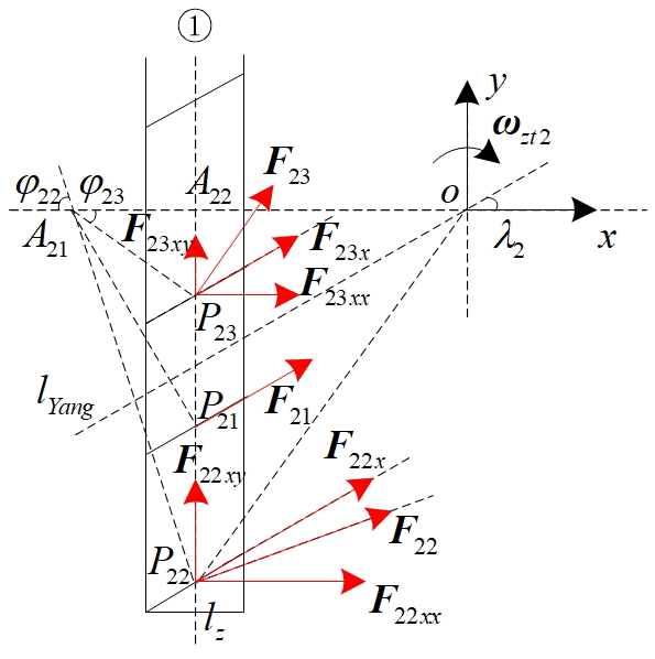
in Fig. 3 is the instantaneous steering center of track (1) of the grounding section of the ideal center-point steering motion. Letting φ2k be the acute angle between the ox axis and the line where A21P2k is, φ2k>0. Then, (for brevity, this is not marked in Fig. 3), , and . The vector decomposition of F2k is conducted along the direction of the roller axis, and the decomposed vector denotes F2kx. F2kx is decomposed along the ox axis and oy axis directions, and the decomposed vectors denote F2kxx and F2kxy. Additionally, , |F2kxx|=|F2kx|cos λ2, and |F2kxy|=|F2kx|sin λ2.
Letting M2k be the steering resistance torque and letting T2k be the driving torque, then and . Analyzing the entire track grounding section (1) of the Type II vehicle, the total steering resistance torque is and the total driving torque is . Given the initial conditions H>0, the expression of the total torque of the grounding section of track (1) of the Type II vehicle is
The analysis of the steering resistance torque and the driving torque of the grounding section of tracks (2)–(4) is similar to that of track (1), and here,
For the Type II vehicle, A21=A23, A22=A24, a21=a23, a22=a24, fT21=fT23, and fT22=fT24.
It can be seen from the above analysis that the two example layouts of Type II shown in Table 1 are equivalent in the center-point steering analysis. The overall center-point steering torque of the Type II vehicle can be expressed as
The analysis of the center-point steering based on the skid conditions of the Type III vehicle is the same as that of the Type II vehicle. The first step of the analysis is to analyze a certain track and then extend the analysis results to other tracks. According to the central symmetry of the Type III layout, the expression of the total torque of the center-point steering of the Type III vehicle is
Supposing that the driving torque of the center-point steering motion of the traditional tracked vehicle is Tc, and the steering resistance torque is Mc, and comparing the expressions in Cheng et al. (2006), with the premise that the direction of the reference frame and the parameters are consistent,
Equation (9) is consistent with the derivation process of the center-point steering motion formula of the Type II vehicle. It can be seen that due to the decomposition of the rollers on the force the driving torque and the steering resistance torque of the Type II vehicle are both the secondary components of the stress moment of the traditional tracked vehicle.
Considering the driving resistance, a model of the center-point steering motion based on the skid conditions of the p-type vehicle is established. Substituting the specific structural parameters of the p-type vehicle and using the numerical solution to solve the equation to obtain Api, Api is used to modify the ideal center-point steering motion equation of the p-type vehicle and to calculate the center-point steering angular velocity reduction coefficient of the p-type vehicle.
4.1 Models of center-point steering motion based on skid conditions
The three types of vehicles have a low-speed uniform center-point steering motion on level ground. According to the plane motion equation of a rigid body,
where Mrp is the driving resistance torque. , where N is the number of tracks of the p-type vehicle and γ the road resistance coefficient. To express Eq. (10) in the form of a function,
When the parameters μ, Bypi, Lp1, λp, Bxpi, and γ in Eq. (11) are known, the equation can be solved and Api can be obtained. Equation (11) is a transcendental equation and an analytical solution cannot be obtained. A numerical iterative solution method is used to find Api.
The roller material of the tracked omni-vehicle is generally hard rubber or polyurethane. The working environment of the tracked omni-vehicle is generally a factory workshop or an outdoor flat road, and a cement road is the common working road. In summary, the parameter values of the ground are set to μ=0.7 and γ=0.04. An example containing specific parameters for each type of the tracked omni-vehicle is chosen, and the absolute lateral offset distance is calculated. Taking vehicles (1), (3), and (7) in Table 2 as examples, A is calculated and a comparative analysis is performed. Table 2 shows the basic parameters of virtual prototypes (1)–(8), where Λ is the length-to-width ratio of the track grounding section.
The relationship between the two sets of parameters {L,A} and {α,A} of the virtual prototypes (1), (2), and (7) is calculated as shown in Fig. 4a and b, where the blue curve is the average value of A for the two tracks on the same side of virtual prototype (3). In engineering design, the design experience of is generally followed because a roller offset angle that is too small or too large will complicate the design and processing of track shoes, and it will affect the anisotropic distribution of the translational velocity and the acceleration of the omni-vehicle (Zhang and Huang, 2015; Yang et al., 2019b; Zhang et al., 2017). Therefore, is taken in Fig. 4b.
It can be seen from Fig. 4 that A increases as L increases and A decreases as α increases. The A value of the Type II and III vehicles is more affected by the change of α and that of the Type I vehicle is less affected. Using a similar drawing method to analyze the relationship between ByA, BxA, and Bxa of the three vehicles, it can be seen that A increases with the increasing By and Bx, and a decreases with the increasing Bx.
4.2 Angular velocity correction of center-point steering motion
The theoretical center-point steering angular velocity ωzt of the three vehicles based on skid conditions can be obtained according to the following formula:
Combining Eqs. (2) and (12), the ratio of ωzt to ωz can be obtained as shown in Eq. (13):
The descent coefficient function is defined as , and , , , , and , where ωzs is the average value of the center-point steering angular velocity of the virtual prototype in the simulation and ωzr is the average value of the center-point steering angular velocity of the physical prototype in the experiment. is the steering angular velocity reduction coefficient of the virtual prototype before and after correction, and is the steering angular velocity reduction coefficient of the physical prototype before and after correction.
Taking the virtual prototypes (1), (3), and (7) in Table 2 as examples, the relationship curve between ψzt and α is drawn as shown in Fig. 5, from which it can be seen that ψzt always decreases with increasing α. It can be seen from Fig. 5 that in the Type II and III vehicles, ψzt is more sensitive to changes in α. When , the ψzt value of virtual prototype (1) is always smaller than that of virtual prototypes (3) and (7). When , the ψzt value of virtual prototype (7) is always smaller than that of virtual prototype (3). This is because the ratio of virtual prototype (7) is smaller than that of virtual prototype (3).
According to the analysis of the translational velocity and the acceleration anisotropy of the tracked omni-vehicle (Zhang and Huang, 2015; Fang et al., 2020; Yang et al., 2019b; Zhang et al., 2017), the optimal value of the roller offset angle in translational motion is rad. For the Type I vehicle, the roller offset angle is set to rad, and this can take into account the best translational motion and center steering motion performance. For the Type II and III vehicles, the offset angle of rad will cause serious slippage in the center-point steering. Therefore, the offset angle should be greater than rad . Additionally, the general value is rad. At this time, the optimal translational performance cannot be considered.
According to the design parameters in Table 2, virtual prototypes (1)–(8) are established in ADAMS, and the center-point steering motion simulation is performed. The correction model is applied to correct ωz. ψzs, ψts and ψs are calculated, and the calculation results are compared and analyzed. Physical prototypes corresponding to the virtual prototypes (1), (2), and (4) are established, and center-point steering motion experiments are conducted. ψzr, ψtr, and ψr are calculated, and the calculation results are compared and analyzed.
5.1 Simulation and analysis
Virtual prototypes established in ADAMS based on Table 2 are shown in Fig. 6.
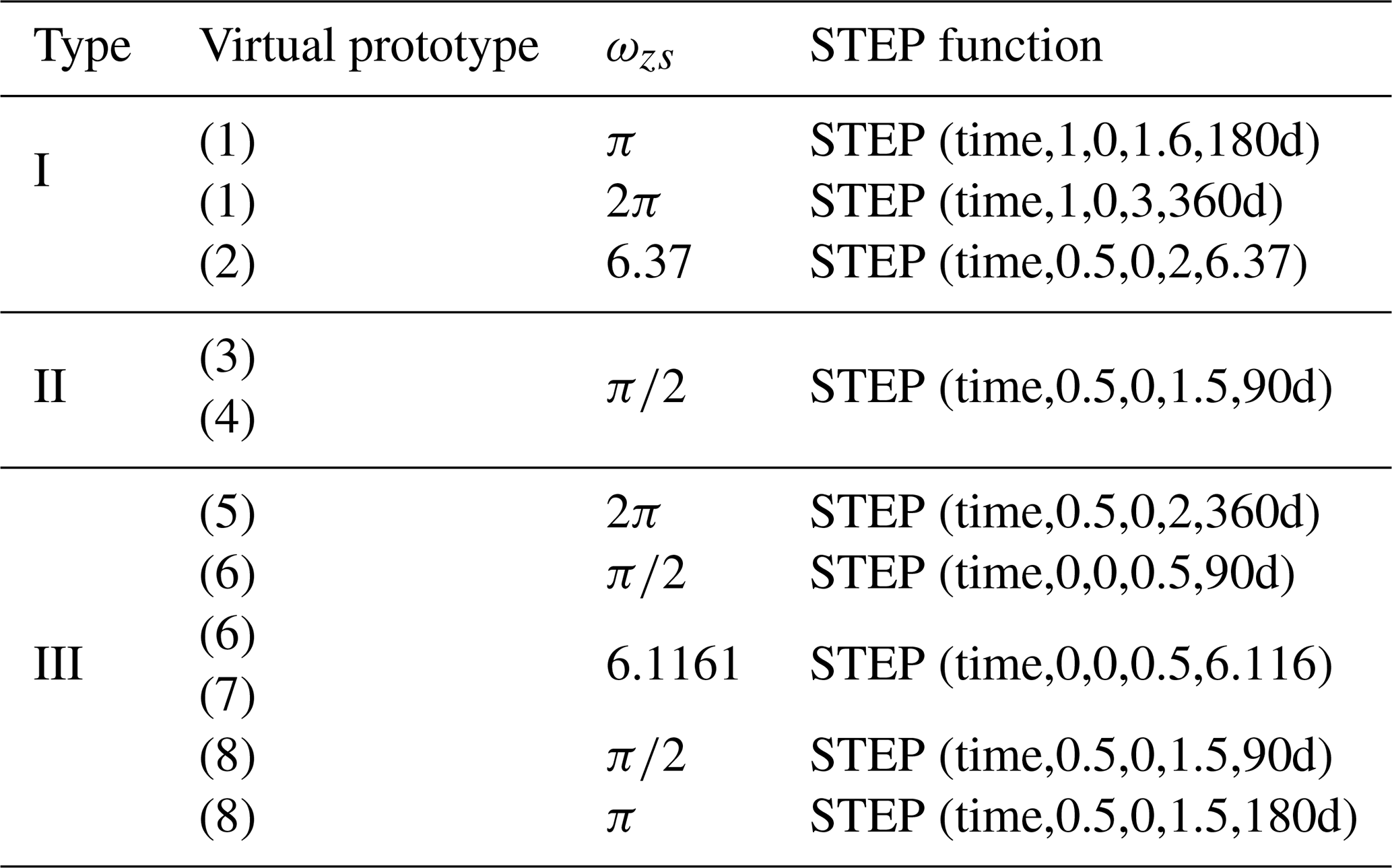
In the simulation, each driving wheel of the same vehicle is driven by the same form of STEP function. The STEP function is applied to the revolute joint of the driving wheel. The syntax of the STEP function is “STEP(x0, x1, h1, x2, h2)”, where x0 represents the independent variable, x1 represents the initial value of the independent variable, h1 represents the initial value of the STEP function, x2 represents the end value of the independent variable, and h2 represents the end value of the STEP function. The STEP functions of the eight virtual prototypes in the simulation are shown in the Table 3.
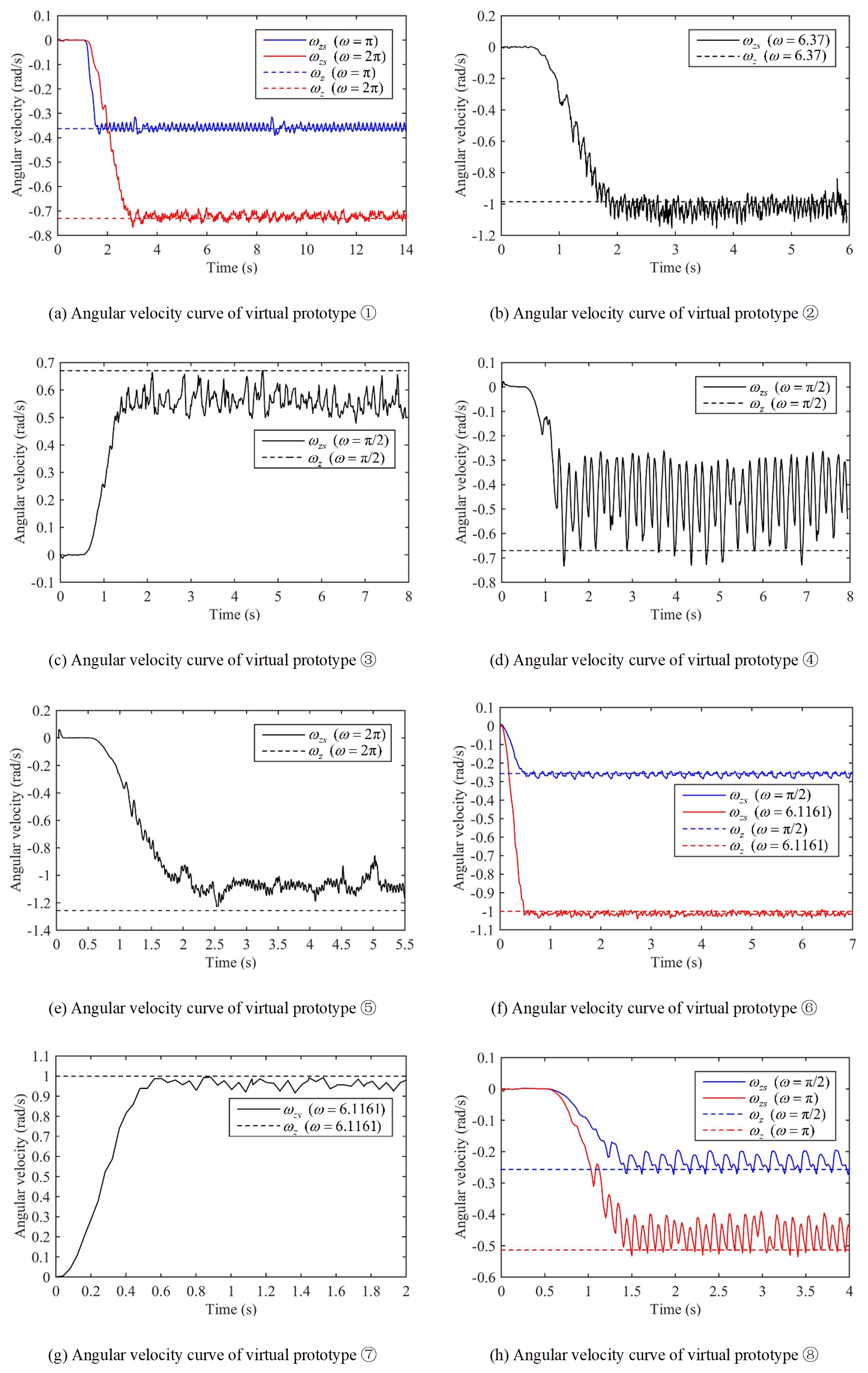
The angular velocity curve of the center-point steering of virtual prototypes (1)–(8) is shown in Fig. 7. The solid line in the figure represents the simulated angular velocity value of the virtual prototype measured. The dotted line represents the calculated ωz value. A positive angular velocity indicates that the virtual prototype turns counterclockwise, and a negative angular velocity indicates that the virtual prototype turns clockwise. Comparing the solid and dashed lines in Fig. 7a–h, it can be seen that the simulated angular velocity values of virtual prototypes (3), (4), (5), and (8) are far from the ideal angular velocity values.
The parameters of the center-point steering of virtual prototypes (1)–(8) obtained by calculation are shown in Table 4.
Table 4Calculation of center-point steering parameters of virtual prototypes (1)–(8).
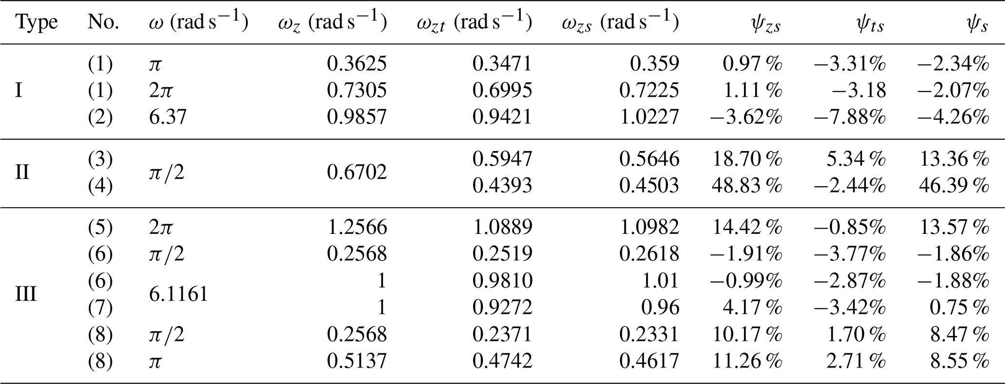
From the information about the virtual prototypes (1), (6), and (8) in Fig. 7 and Table 4, it can be seen that the difference in the speed of the driving wheels does not cause drastic changes in the values of parameters such as ψzs and ψts, which shows the correctness of the built simulation model and the modified model. It can be seen from Fig. 7 and Table 4 that the ψzs values of virtual prototypes (1) and (2) are relatively small because of the low slippage characteristics of the Type I vehicle. The ψzs value of virtual prototype (6) is small because the L1 value of (6) (as shown in Table 2) is small.
Compared with ψs in Table 4, it can be seen that the correction effects of virtual prototypes (1), (2), and (6) are not good, but the corrections increase the absolute values of the errors. The correction effects of virtual prototypes (7) and (8) are not obvious, and the absolute values of the errors are slightly reduced after correction. The correction effects of virtual prototypes (3)–(5) are better, and the absolute value of the error is greatly reduced after correction. The reason for the above correction difference is that the Λ values of virtual prototypes (1), (2), and (6) (as shown in Table 2) are small, which makes it impossible to ignore the influence of the track width on center-point steering, which contradicts the assumption (4) in Sect. 2. According to design experience, the condition of the assumption (4) is Λ>10. From the perspective of the three types, it can be seen that the modified model is generally suitable for theoretical calculation and the correction of Type II and III vehicles, and it is generally not necessary to modify the Type I vehicle.
5.2 Experiments and analysis
Physical prototypes (1), (2), and (4) corresponding to the virtual prototypes (1), (2), and (4), respectively, in Table 2 and Fig. 6 are established and center-point steering motions are conducted, as shown in Fig. 8. The wheels of the physical prototypes (1), (2), and (4) are all hard rubber, and the road conditions are all dry cement roads. The center-point steering process of physical prototypes (1) and (2) is smooth. In the process of center-point steering, the shift of the steering center of physical prototype (4) is more obvious, and the tracks near the vehicle body vibrated more than those far from the vehicle body do, and the phenomenon of blocking in motion manifests.
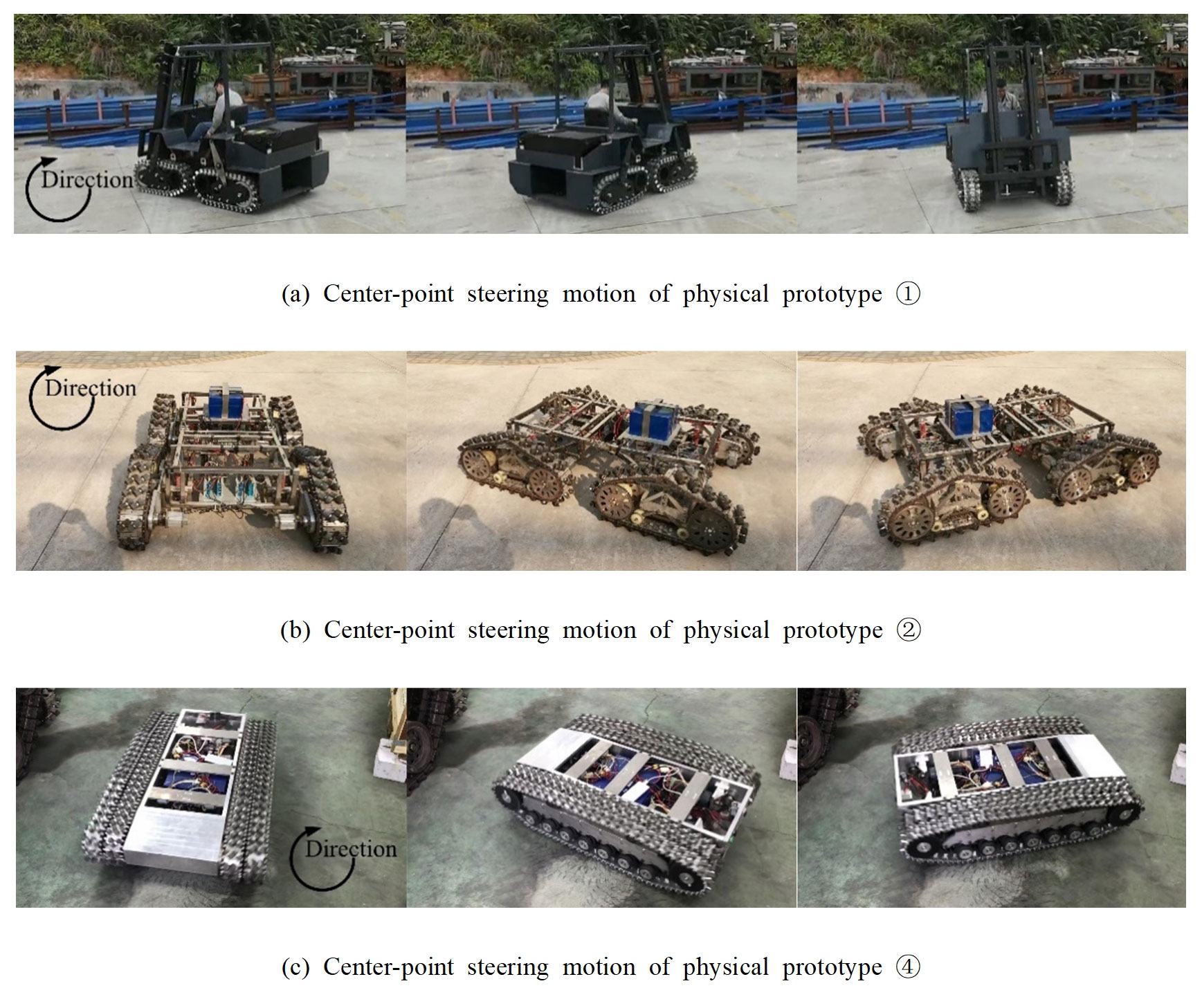
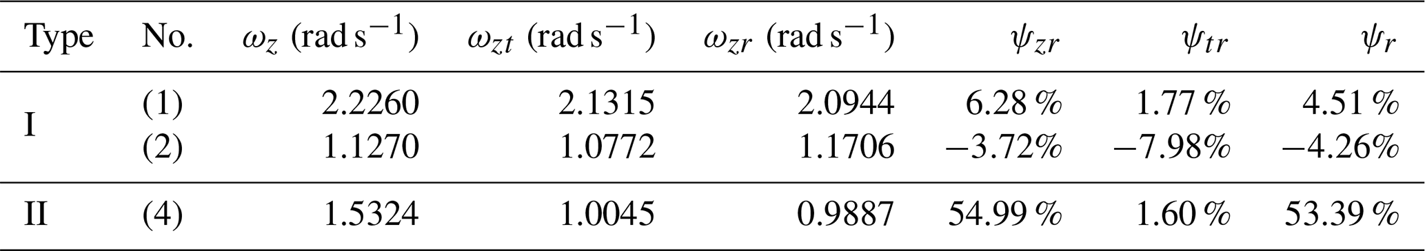
According to Eqs. (2), (12), and (13), ωz, ωzt, ψzr, ψtr, and ψr are calculated as shown in Table 5. Compared with ψr, it can be seen that the correction model has a positive correction effect on physical prototypes (1) and (4), reducing the speed error, and it has a significant correction effect on physical prototype (4). The correction model has a negative correction effect on physical prototype (2), but it increases the speed error. The conclusion obtained with the analysis of ψr is consistent with the conclusion obtained with the analysis of ψs. It can be seen that the correction model and the virtual prototypes are correct.
Table 5Data for center-point steering motion of physical prototypes.
Taking three typical layouts as examples, in this study, the center-point steering motion of a tracked omni-vehicle based on skid conditions is analyzed, and the analysis results are compared and analyzed using the simulation and experimental data. The following conclusions are drawn.
-
Compared with traditional tracked vehicles, the rectangular layout of a tracked omni-vehicle has a horizontal original offset of the steering pole in the center-point steering motion. This original offset is related to the roller offset angle and the track grounding length of the vehicle. The parameters are directly related.
-
In the center-point steering motion, due to the force decomposition of the rollers, the driving torque and the steering resistance torque of the Type II and III vehicles are the secondary components of the corresponding torque of the traditional tracked vehicle.
-
For the case of the same roller offset angle, in center-point steering, the slips of the Type II and III vehicles are more serious than that of the Type I vehicle. When higher requirements for the center-point steering exist in the design stage, the Type I vehicle should be selected for structural design first. When comprehensively considering the translation and center-point steering motion performance, the optimal value of the roller offset angle of the Type I vehicle is generally rad. The optimal value of the roller offset angle of the hybrid and centripetal layout vehicles should generally be greater than rad, and rad is usually chosen as a compromise.
-
The analysis of the simulation and experimental data shows that the reduction coefficient of the center-point steering angular velocity of the tracked omni-vehicle given in this article can play a corrective role. The correction effect on the Type II and III vehicles is more obvious than that of the Type I vehicle. The corrective effect is obvious when the length-to-width ratio of the track grounding is relatively large.
Based on the research in this article, the following four directions are worthy of further research in the future.
-
Researchers should consider studying equations of motion such as Eq. (7) from the perspective of force and power, e.g., by analyzing the relationship between the power of the vehicle's driving wheel and center-point steering radius, and obtaining the law of the vehicle's steering power.
-
Researchers should consider reducing the number of assumptions in Sect. 3 and conduct a more detailed study on the center-point steering motion of the tracked omni-vehicle. For example, researchers do not ignore the width of the track grounding section or study the center-point steering motion when the position of the center of gravity changes.
-
Researchers should consider the influence of the ground and soil on the center-point steering motion, explore the vehicle's moving capabilities on unstructured roads, and expand the application environment of the vehicle.
-
Different degrees of velocity and trajectory deviations will occur in the center-point steering motion. It is necessary to study the control methods to correct this deviation and find the control laws and methods to improve the steering performance.
| a | relative offset distance of steering pole (m) |
| A | absolute lateral offset distance of steering pole (m) |
| Bx, By | length of projection of distance between center of track and center of vehicle in the x axis |
| and y axis directions (m) | |
| fT | total torque of grounding section of track (N m) |
| fz | total center-point steering torque (N m) |
| F | reverse force vector |
| Fx | component force of F along axis of roller |
| Fxx | component force of Fx along ox axis direction |
| Fxy | component force of Fx along oy axis direction |
| g | acceleration due to gravity (m s−2) |
| H | half of length of track grounding section (m) |
| Jω | Jacobian matrix |
| l | distance between center of track and center of vehicle (m) |
| L | length of single track grounding section (m) |
| m | vehicle mass (kg) |
| M | steering resistance torque (N m) |
| Mc | steering resistance torque of traditional tracked vehicle (N m) |
| Mr | resistance moment during driving (N m) |
| N | number of tracks of p-type vehicle |
| r | radius of driving wheel (m) |
| T | steering driving torque (N m) |
| Tc | steering driving torque of traditional tracked vehicle (N m) |
| vx | translational velocity in x axis direction (m s−1) |
| vy | translational velocity in y axis direction (m s−1) |
| Vj | absolute velocity vector |
| Vq | following velocity vector |
| Vx | relative velocity vector |
| Greek symbols | |
| α | roller offset angle (rad) |
| β | angle between center of track and center of vehicle (rad) |
| γ | road resistance coefficient |
| η | angle between roller axis and vehicle coordinate system (rad) |
| θ | angle between coordinate system of track and coordinate system of vehicle (rad) |
| λ | absolute value of roller offset angle (rad) |
| Λ | length-to-width ratio of track grounding section |
| μ | steering resistance coefficient |
| φ | acute angle between ox axis and straight line connecting point on ground roller |
| and instantaneous steering center (rad) | |
| ψ | descent coefficient function |
| ψr | steering angular velocity reduction coefficient of physical prototype before and after correction |
| ψs | steering angular velocity reduction coefficient of virtual prototype before and after correction |
| ω | angular velocity of driving wheel (rad s−1) |
| ωz | angular velocity of center-point steering motion without considering slippage (rad s−1) |
| ωzr | average value of center-point steering angular velocity of physical prototype in experiment (rad s−1) |
| ωzs | average value of center-point steering angular velocity of virtual prototype in simulation (rad s−1) |
| ωzt | angular velocity of center-point steering motion considering slippage (rad s−1) |
| Subscripts | |
| i | different tracks on same tracked omni-vehicle, |
| k | different roller grounding points on same track, |
| p | different types of tracked omni-vehicle, |
All the data used in this paper can be obtained from the corresponding author on request.
Conceptualization was by YF and YZ. Data curation was done by YF, TH, and MY. Formal analysis was made by YF. Investigations were carried out by YF, TH, and MY. The methodology was by YF and YZ. Project administration was performed by YZ and YS. Resources came from YZ. Software came from YF. Supervision was by YZ and YS. Visualization was by YF, TH, and MY. YF wrote the original draft. Writing, review, and editing were done by YZ and YS.
The authors declare that they have no conflict of interest.
We thank LetPub (https://www.letpub.com, last access: 1 April 2021) for its linguistic assistance during the preparation of the manuscript.
This research has been supported by the State Administration for Science, Technology and Industry for National Defense (grant no. 2015ZB15).
This paper was edited by Daniel Condurache and reviewed by three anonymous referees.
Cao, A.: Omni-directional all-terrain six-wheeled tracked vehicle, Patent: National Intellectual Property Administration, PRC, CN106240663B, Beijing, China, 2018.
Chen, P., Mitsutake, S., Isoda, T., and Shi, T.: Omni-directional robot and adaptive control method for off-road running, IEEE Trans. Robot. Autom., 18, 251–256, https://doi.org/10.1109/TRA.2002.999654, 2002.
Cheng, J., Gao, L., and Wang, H.: Steering analysis of tracked vehicles based on skid condition, Chinese J. Mech. Eng., 42, 192–195, 2006.
Cheng, J., Gao, L., Wang, H., and Liu, F.: Analysis on the Steering of Tracked Vehicles, Acta Armamentarii, 28, 1110–1115, https://doi.org/10.3321/j.issn:1000-1093.2007.09.017, 2007.
Clavien, L., Lauria, M., and Michaud, F.: Instantaneous centre of rotation based motion control for omnidirectional mobile robots with sidewards off-centred wheels, Rob. Auton. Syst., 106, 58–68, https://doi.org/10.1016/j.robot.2018.03.014, 2018.
Fang, Y., Zhang, Y., Li, N., and Shang, Y.: Research on a medium-tracked omni-vehicle, Mech. Sci., 11, 137–152, https://doi.org/10.5194/ms-11-137-2020, 2020.
Guan, J. and Yuan, K.: Omni-directional moving transmission continuous track, Patent: National Intellectual Property Administration, PRC, CN106515886B, Beijing, China, 2019.
Hua, J. and Zhang, C.: Four-axis drive crawler wheel type forklift, Patent: National Intellectual Property Administration, PRC, CN110356483A, Beijing, China, 2019.
Huang, T., Zhang, Y., Tian, P., Yan, N., and Zhang, J.: Design & kinematics analysis of a tracked omnidirectional mobile platform, J. Mech. Eng., 50, 206–212, https://doi.org/10.3901/JME.2014.21.206, 2014.
Karavaev, Y. L. and Kilin, A. A.: Nonholonomic dynamics and control of a spherical robot with an internal omniwheel platform: Theory and experiments, Proc. Steklov Inst. Math., 295, 158–167, https://doi.org/10.1134/s0081543816080095, 2017.
Li, X., Xie, F., Liu, D., Huang, L., Ye, Q., and Yuan, K.: Omni-directional moving track, Patent: National Intellectual Property Administration, PRC, CN102756764A, Beijing, China, 2012.
Liu, Y., Huang, T., Li, H., and Yan, Y.: Combined crawler belt walking mechanism with omni-directional movement and platform thereof, Patent: National Intellectual Property Administration, PRC, CN108163072A, Beijing, China, 2018.
Ma, D., Chen, D., Li, M., Zhou, X., and Chen, Z.: Qxcomm technology's track based on mecanum wheel, Patent: National Intellectual Property Administration, PRC, CN204821767U, Beijing, China, 2015.
Madhushani, T. W. U., Maithripala, D. H. S., Wijayakulasooriya, J. V., and Berg, J. M.: Semi-globally exponential trajectory tracking for a class of spherical robots, Automatica, 85, 327–338, https://doi.org/10.1016/j.automatica.2017.07.060, 2017.
Mortensen Ernits, R., Hoppe, N., Kuznetsov, I., Uriarte, C., and Freitag, M.: A new omnidirectional track drive system for off-road vehicles, 2017 XXII Int. Conf., MATERIAL Handl. Constr. Logist., 105–110, 2017.
Park, Y. K., Lee, P., Choi, J. K., and Byun, K. S.: Analysis of factors related to vertical vibration of continuous alternate wheels for omnidirectional mobile robots, Intell. Serv. Robot., 9, 207–216, https://doi.org/10.1007/s11370-016-0196-3, 2016.
Roh, S.-G., Taguchi, Y., Nishida, Y., Yamaguchi, R., and Hirose, S.: Development of the portable ground motion simulator of an earthquake, in: 2013 IEEE/RSJ International Conference on Intelligent Robots and Systems (IROS), 5339–5344, https://doi.org/10.1109/IROS.2013.6697129, 2013.
Singh, A., Sachdeva, E., Sarkar, A., and Krishna, K. M.: COCrIP: Compliant omniCrawler in-pipeline robot, in: 2017 IEEE/RSJ International Conference on Intelligent Robots and Systems (IROS), IEEE, 5587–5593, https://doi.org/10.1109/IROS.2017.8206446, 2017.
Song, H., Gao, L., Li, J., and Yao, X.: Correction and Experiment of Steering Performance Index of Tracked Vehicles, J. Acad. Armored Force Eng., 22, 65–68, https://doi.org/10.3969/j.issn.1672-1497.2008.06.016, 2008.
Song, H., Yao, X., Gao, L., and Yu, K.: Correction and experiment of zero radio turning index of tracked vehicle, Veh. Power Technol., 3, 5–8, 17, https://doi.org/10.3969/j.issn.1009-4687.2009.03.002, 2009.
Tadakuma, K., Tadakuma, R., and Berengueres, J.: Tetrahedral Mobile Robot with Spherical Omnidirectional Wheel, J. Robot. Mechatronics, 20, 125–134, https://doi.org/10.20965/jrm.2008.p0125, 2008.
Tadakuma, K., Tadakuma, R., Nagatani, K., Yoshida, K., Aigo, M., and Shimojo, M.: Throwable tetrahedral robot with transformation capability, 2009 IEEE/RSJ Int. Conf. Intell. Robot. Syst., 2801–2808, https://doi.org/10.1109/IROS.2009.5354196, 2009.
Tadakuma, K., Tadakuma, R., Higashimori, M., and Kaneko, M.: Robotic finger mechanism equipped omnidirectional driving roller with two active rotational axes, in: 2012 IEEE International Conference on Robotics and Automation, 3523–3524, https://doi.org/10.1109/ICRA.2012.6225378, 2012.
Tadakuma, K., Ogata, H., Higashimori, M., Kaneko, M., Tadakuma, R., and Berengueres, J.: Torus omnidirectional driving unit mechanism realized by curved crawler belts, Proc.-IEEE Int. Conf. Robot. Autom., 2567, https://doi.org/10.1109/ICRA.2014.6907224, 2014.
Tadakuma, K., Takane, E., Fujita, M., Nomura, A., Komatsu, H., Konyo, M., and Tadokoro, S.: Planar omnidirectional crawler mobile mechanism – development of actual mechanical prototype and basic experiments, IEEE Robot. Autom. Lett., 3, 395–402, https://doi.org/10.1109/LRA.2017.2739101, 2017.
Takane, E., Tadakuma, K., Shimizu, T., Hayashi, S., Watanabe, M., Kagami, S., Nagatani, K., Konyo, M., and Tadokoro, S.: Basic Performance of Planar Omnidirectional Crawler during Direction Switching using Disturbance Degree of Ground Evaluation Method, IEEE Int. Conf. Intell. Robot. Syst., 2732–2739, https://doi.org/10.1109/IROS40897.2019.8968507, 2019.
Tong, Z.: A motion study of the omnidirectional mobile robot, Master Degree, Shenyang Aerospace University, Shen Yang, Liao Ning, China, 2017.
Wang, X.: Theory and application of Mecanum wheel based omni-directional mobile, Southeast University Press, Jiang Su, 2018.
Xing, Q., Wu, H., Liu, Y., Yang, C., Zhu, Y., Liao, H., Cheng, S., and Wu, J.: Novel Mecanum wheel creeper truck, Patent: National Intellectual Property Administration, PRC, CN108016518A, Beijing, China, 2018.
Yang, H., Zhang, Y., Fang, Y., Cui, Z., and Dong, Z.: Analysis and Simulation of Omnidirectional Platform in Complex Environments, Fire Control Command Control, 44, 135–138, https://doi.org/10.3969/j.issn.1002-0640.2019.09.026, 2019a.
Yang, H., Zhang, Y., Huang, T., Fang, Y., Zhang, Q., and Zhang, J.: Motion analysis of novel track omnidirectional platform, J. Zhejiang Univ. Sci., 52, 1345–1353, https://doi.org/10.3785/j.issn.1008-973X.2018.07.015, 2019b.
Yang, Y., Yang, G., Tian, Y., Zheng, T., Li, L., and Wang, Z.: A robust and accurate SLAM algorithm for omni-directional mobile robots based on a novel 2.5D lidar device, 2018 13th IEEE Conf. Ind. Electron. Appl., 2123–2127, https://doi.org/10.1109/ICIEA.2018.8398060, 2018.
Yu, C., Lin, J., and Liu, B.: Crawler-type omnidirectional mobile platform, Patent: National Intellectual Property Administration, PRC, CN210310616U, Beijing, China, 2020.
Zhang, J.: Omni-directional tracked vehicle, Patent: National Intellectual Property Administration, PRC, CN108583704A, Beijing, China, 2018.
Zhang, X., Yang, S., Sun, L., and Zhang, J.: Novel all-round track moving platform structure, Patent: National Intellectual Property Administration, PRC, CN205769664U, Beijing, China, 2016.
Zhang, Y.: Omnidirectional mobile track, Patent: National Intellectual Property Administration, PRC, CN103043128B, Beijing, China, 2017.
Zhang, Y. and Huang, T.: Research on a tracked omnidirectional and cross-country vehicle, Mech. Mach. Theory, 87, 18–44, https://doi.org/10.1016/j.mechmachtheory.2014.12.016, 2015.
Zhang, Y. and Yang, H.: Designing of a small reconnaissance platform based on omnidirectional chassis, Fire Control Command Control, 43, 130–134, https://doi.org/10.3969/j.issn.1002-0640.2018.07.024, 2018.
Zhang, Y., Huang, T., Zhang, S., and Zhang, J.: Analysis about steering slip power ratio of a tracked omnidirectional mobile platform, Acta Armamentarii, 36, 1562–1568, https://doi.org/10.3969/j.issn.1000-1093.2015.08.026, 2015.
Zhang, Y., Yang, H., Huang, T., Zhang, S., and Fang, Y.: Analysis about motion of centripetal tracked omnidirectional mobile platforms, Acta Armamentarii, 38, 2309–2320, https://doi.org/10.3969/j.issn.1000-1093.2017.12.003, 2017.
Zhang, Y., Fang, Y., Yang, H., Cui, Z., and Shi, H.: Kinematics Analysis & Simulation of a Tracked Omnidirectional Mobile Platform, Fire Control Command Control, 44, 132–136, https://doi.org/10.3969/j.issn.1002-0640.2019.06.026, 2019.
- Abstract
- Introduction
- Typical layout and ideal kinematics equation
- Center-point steering analysis based on skid conditions
- Models and angular velocity correction
- Center-point steering analysis based on skid conditions
- Conclusions
- Appendix A: List of symbols
- Data availability
- Author contributions
- Competing interests
- Acknowledgements
- Financial support
- Review statement
- References