the Creative Commons Attribution 4.0 License.
the Creative Commons Attribution 4.0 License.
 | 30 Mar 2021
Design and analysis of a light electric vehicle
Chang-Sheng Lin
Chang-Chen Yu
Yue-Hao Ciou
Yi-Xiu Wu
Chuan-Hsing Hsu
Yi-Ting Li
This paper discusses a systematic vehicle design process in which light weight is taken as the vehicle design objective, and the designed frame is analyzed in detail. The load condition of a vehicle under different circumstances is calculated according to the distances from the front and rear wheels to the centroid position. The stress on the components in the condition is analyzed by finite element analysis, the steering geometry of the vehicle is analyzed, and the vehicle's turning angle and radius are designed. The displacement of the vehicle under a load is calculated by rigidity analysis to determine the stability of the vehicle in motion. The experimental modal analysis of the real frame and the finite element method are verified mutually for the electric vehicle body-in-white (BIW) manufacturing process to determine the consistency of model formation and the real frame. In terms of the circuit design, we used no-fuse switches and fuses to provide overcurrent protection for the main power supply, and the chip is combined with an optically coupled circuit and current sensor, which is driven by a restriction controller for protection. Moreover, a solid-state relay (SSR) is used for current protection and for controlling the forward/reverse rotation of the motor.
- Article
(8791 KB) - Full-text XML
- BibTeX
- EndNote


At present, with the advancement of society, electric vehicles have been popularized in various countries' markets. With the rise of recreational sports, various activities are held all over the world. Electric vehicle races show lightweight vehicle bodies with an adequate sense of speed, and the feeling is fed back to the driver by the vehicle, which cannot be achieved by most recreational sports. Therefore, building a low-cost and simple light electric racing car is the design objective for this vehicle.
In this vehicle design, the designed vehicle's turning radius is obtained by steering geometry analysis (Afkar et al., 2012) and is judged by whether the design could pass every curve in the racing field smoothly (Pourasad et al., 2016). The loads on the front and rear axles of the vehicle in constant speed motion, acceleration, braking, and cornering are calculated by front and rear axle load analysis. The stress on the axle parts is analyzed by finite element analysis, according to the calculation result, to ensure that the part would not suffer from plastic deformation under the loading condition. The rigidity of the frame before and after being equipped with stiffeners is analyzed to check whether the reinforcement design could enhance the rigidity effectively. Finally, modal analysis is performed for the frame, and the modal frequency and vibration mode shape are verified mutually by experimental modal analysis to guarantee the model verification.
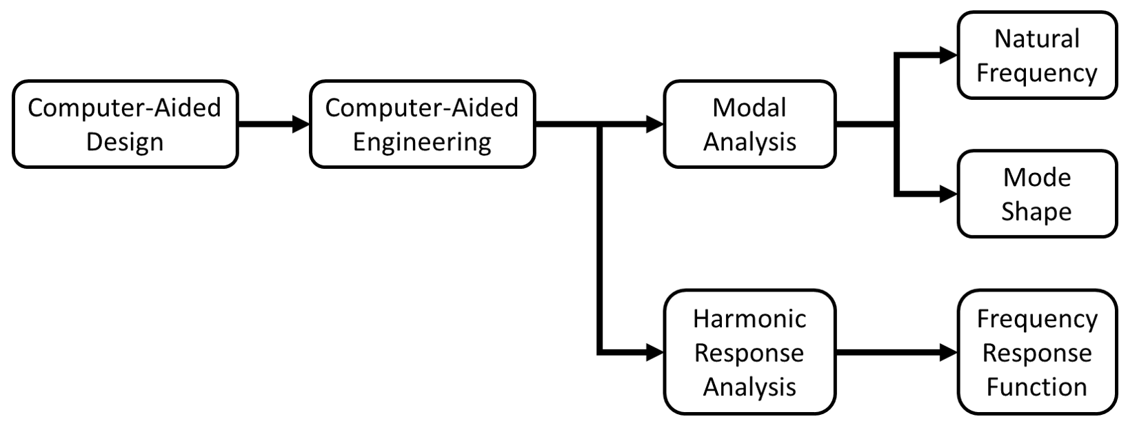
The power and safety switches of the electric vehicle are designed based on a power requirement evaluation, and the steering geometry is designed and analyzed so that the electric vehicle can pass every curve in the racing fields smoothly. The loads on the front and rear axles of the vehicle in constant speed motion, acceleration, braking, and cornering are calculated using front and rear axle load analysis, and the stress on the axle part is analyzed by finite element analysis to ensure that the part would not suffer from plastic deformation under different loading conditions. The rigidity of the frame before and after being equipped with stiffeners is analyzed to check whether the design could enhance the rigidity effectively (Marzbanrad et al., 2015). Finally, modal analysis is performed on the frame, and the modal frequency and vibration mode shape are verified mutually by experimental modal analysis to guarantee the model verification. The process of analysis is shown in Fig. 1.

3.1 Power system
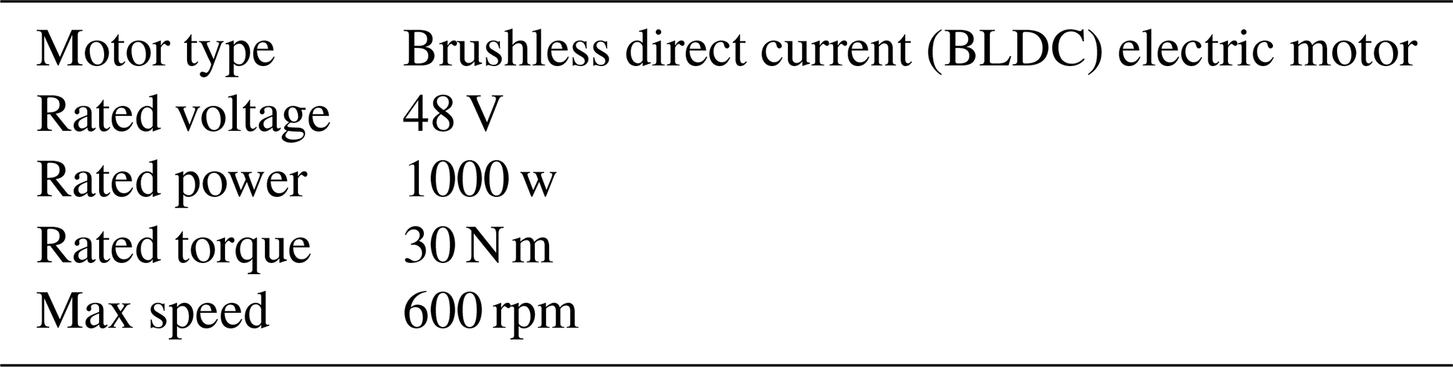
The style of the light electric vehicle is that it is designed with two front wheels and one rear wheel. In order to improve high transmission efficiency and high torque, a hub motor is installed on the rear wheel to directly drive the vehicle without a gear-reduction mechanism. The hub motor is an outer rotor brushless direct current (DC) motor, and its basic specifications are shown in Table 1.
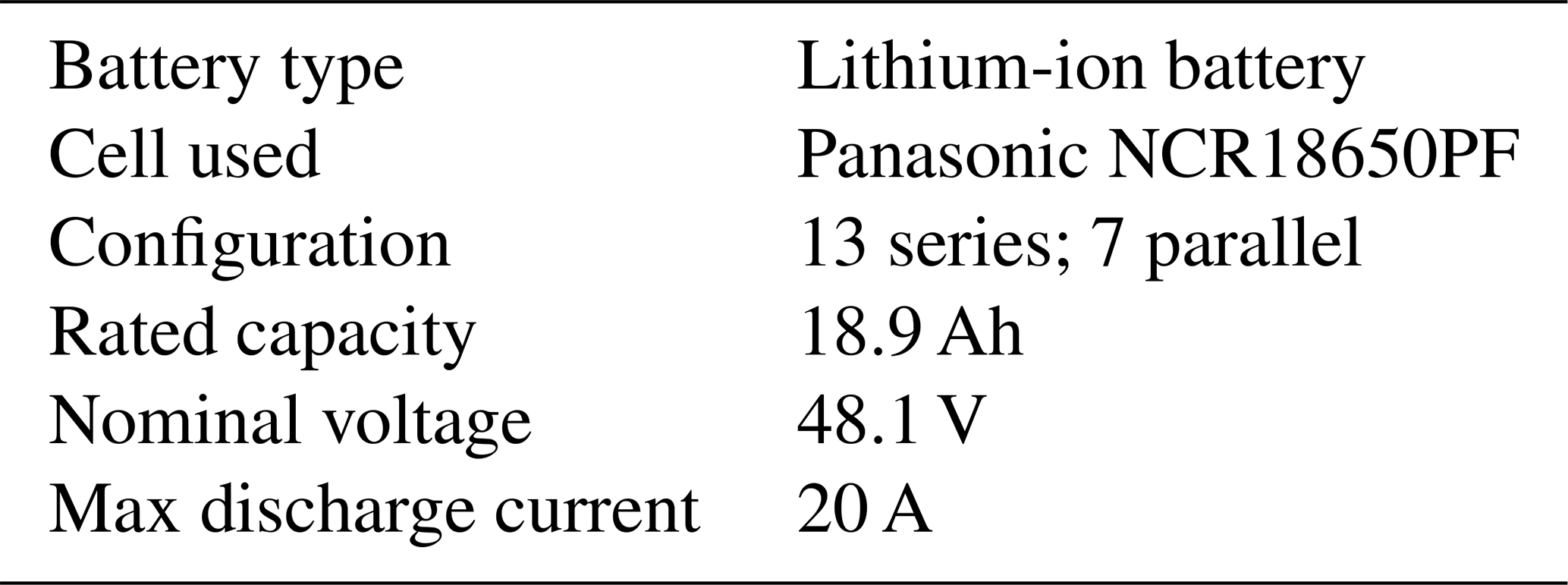
Figure 2 shows the electrical frame of the power system, mainly including the battery, inverter, hub motor, etc. This study uses a high energy density lithium battery as the energy source of the electric vehicle, and its specifications are shown in Table 2. The motor inverter uses a commercially available driver and directly determines the output power of hub motor through the accelerator pedal (ACCP).
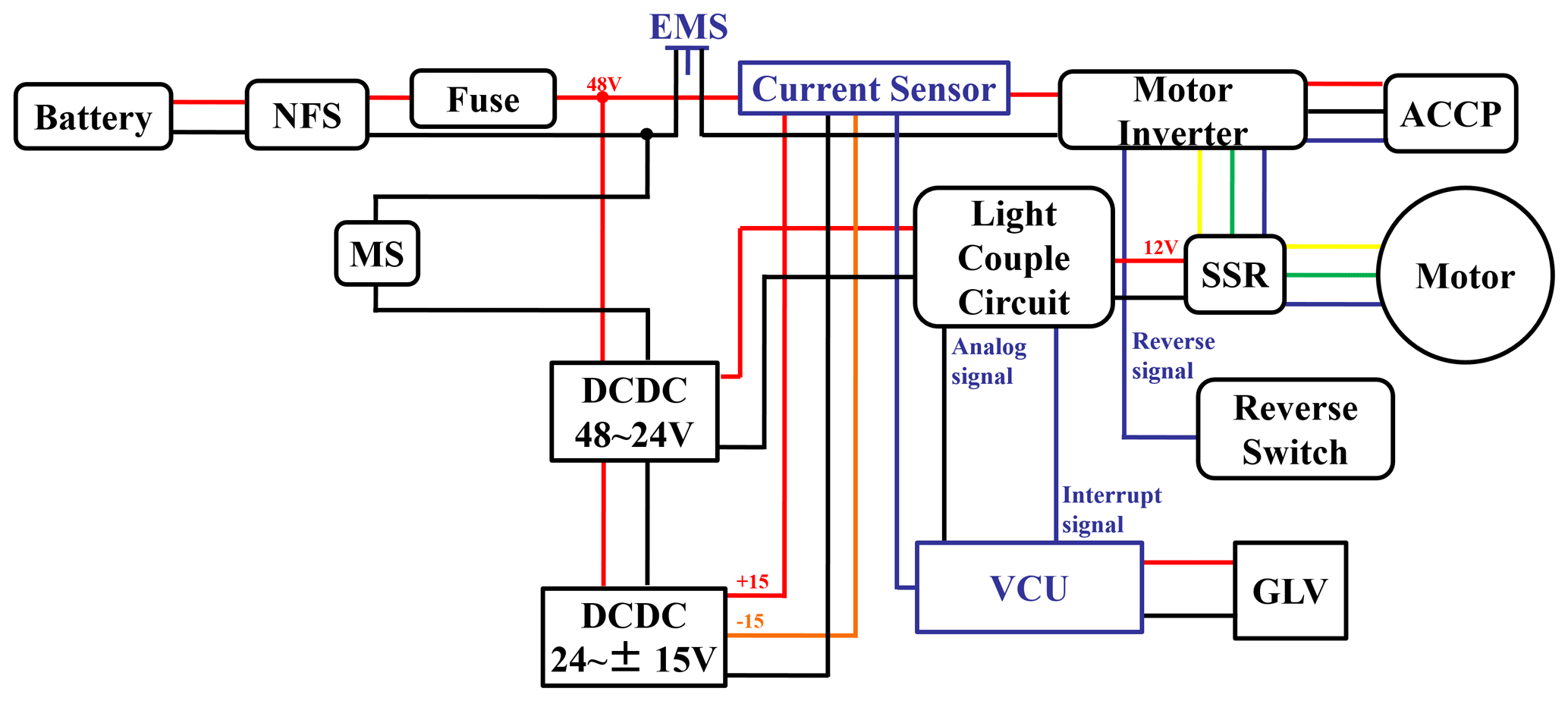
In order to meet the electrical safety requirements of an electric vehicle, it is necessary to establish a complete management strategy for battery safety issues. Therefore, real-time diagnosis of high and low voltage protection, short circuit faults, etc. is necessary to make accurate judgments and automatically take effective protective measures before or when power system faults occur to effectively protect the lives and property safety of drivers. In the design of the emergent protection measures, the main switch is set as a no-fuse switch (NFS) to control the power supply of the automotive electrical system. There are emergency switches (EMSs) installed on the steering wheel and on the back of the seat so that the driver or people outside the car can cut off the power in an emergency. In terms of overload protection function, the vehicle control unit (VCU) is responsible for monitoring the battery voltage and current value. If an abnormal situation occurs, it will transmit the control signal to the optically coupled circuit and then drive the solid-state relay (SSR) to cut off the motor's three-phase power wires (labeled as a U–V–W phase sequence).
3.1.1 Expected performance of the electric vehicle
In the initial design stage, there are two main parts that affect the weight estimation. The first part is the design goal. This vehicle design is aimed drivers participating in leisure activities, so performance will be more important, but, at the same time, safety will be too; any part of the design that touches the target must be compromised, including weight. One of the design goals is to reduce part of the mass for better acceleration performance of the motor. The second goal is the system design priority. In the process of making the finished product, we cannot ensure that all components can be produced independently. To achieve a balance between production cost and time, the control of the maximum weight is the autonomy of the fulfillable goal of the production parts, and components that compromise on production cost and time will be provided by reliable suppliers. Since the components provided by the supplier have only low design flexibility, the corresponding weight must be given priority in the estimation.
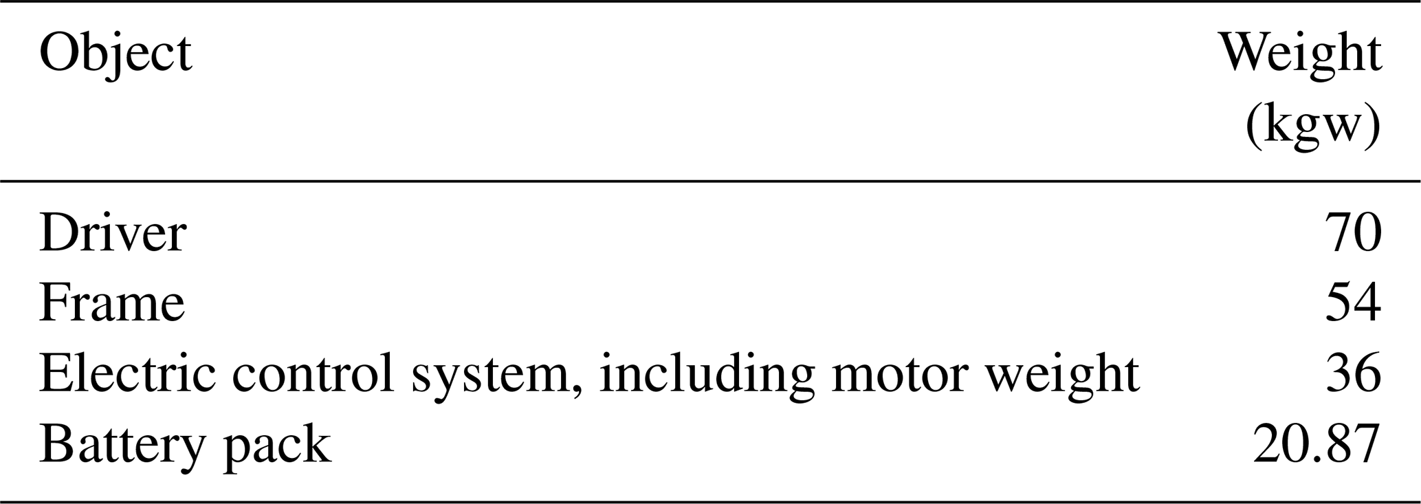
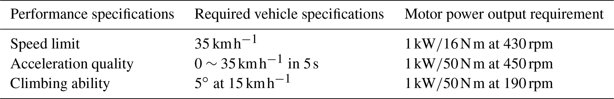
The remaining weight will be designed and produced by the original parts to achieve the initial design weight to ensure the performance of the finished product. The design performance is controlled within a smaller error range. We have added up the weight of the components provided by the supplier, and the estimated driving weight is 70 kg, and the remaining distance target is 54 kg, which is a component designed and produced by ourselves. The parameters associated with the weight of the designed car are listed in Table 3. According to the condition of the racing track and the regulations of the race, we hoped that the speed could be up to 15 km h−1 on the steepest racing track. The expected performance is determined according to the conditions shown in Table 4.
Table 3The parameters associated with the weight of the designed car.
3.1.2 Elementary calculation
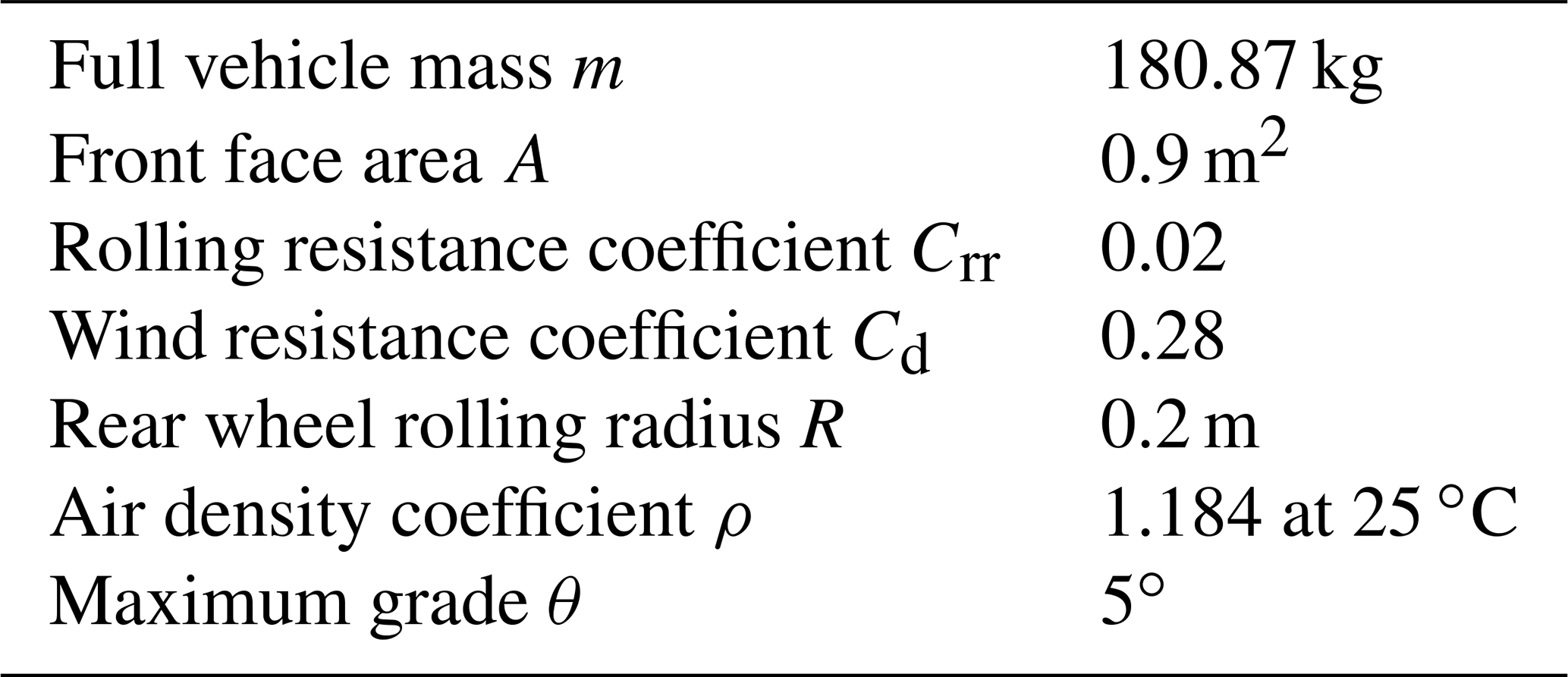
The following basic parameters are obtained according to our designed vehicle and the racing track conditions, as shown in Table 5.
The vehicle dynamics equation could be expressed as follows:
The torsion equation is deduced from Eq. (1) to calculate the required motor torque of the designed vehicle, which is expressed as follows:
The parameters in Table 2 are substituted in Eq. (2) to calculate the required torsion for a flat road start (0∘ slope) and an acceleration of 1.39 m s−2 in the expected performance index (air drag not considered; start on 0∘ slope, so there is no g). The starting torsion is T=53.93 N m, which the torsion for maintaining the speed of 15 km h−1 on 5∘ slope (air drag not considered; acceleration is 0). For a traveling torsion on 5∘ slope, T=48.6 N m, and the required motor speed is RPM=198 rpm, according to 15 km h−1 of the performance index. The propulsion motor is selected according to the aforesaid torsion and the corresponding RPM level.
3.1.3 Capacity estimation
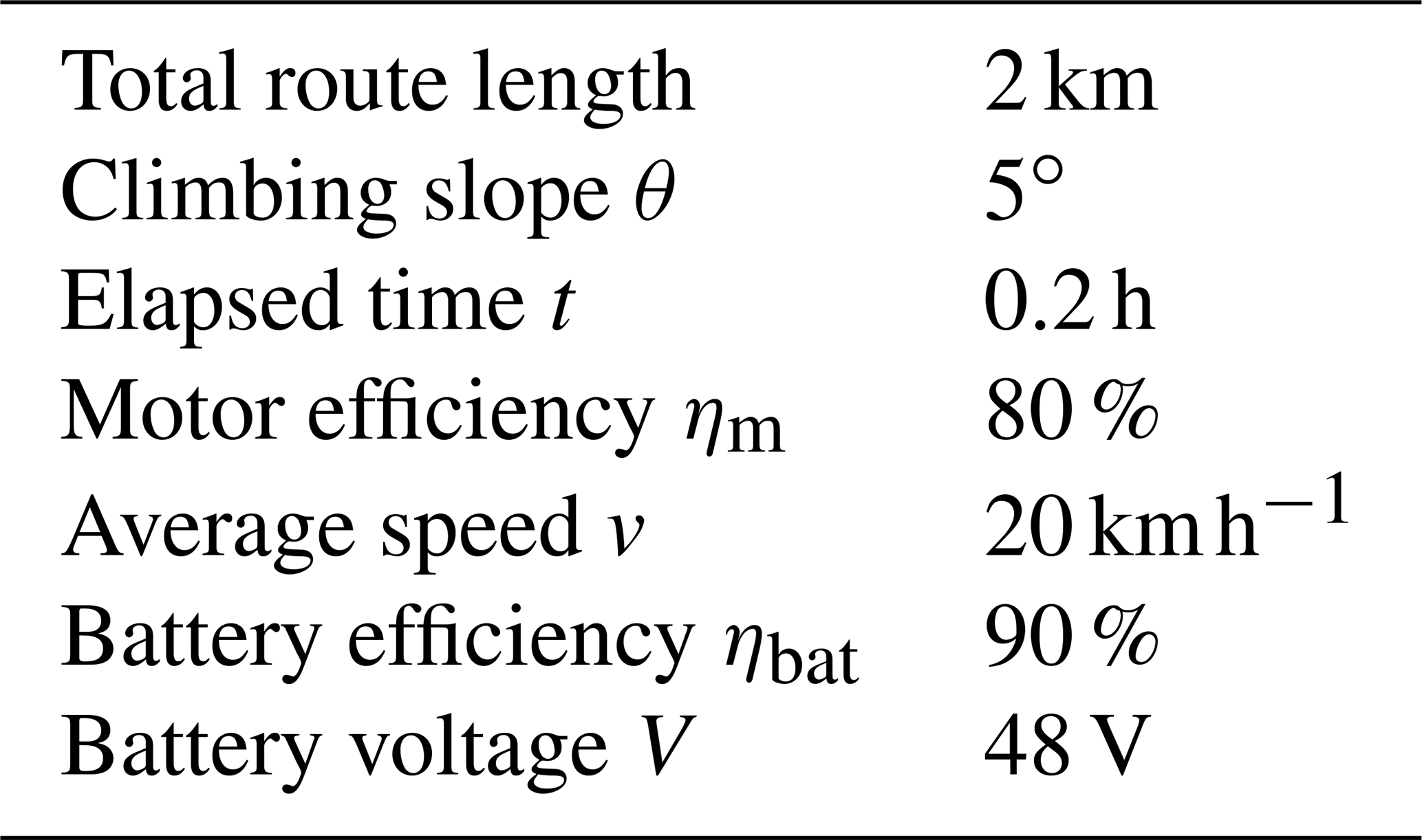
According to the racing track and regulations of this match, the following parameters are studied, and the minimum limit of our battery pack specification is calculated by the equation listed in Table 6.
To obtain the motor power, the relation of the value to the torsion and speed is as follows:
The calculated minimum motor torque of 53.93 N m and the required motor speed of 198 rpm are put into Eq. (3) to obtain the motor power P=716 W.
In order to obtain the motor discharging current, the relation of the value to the battery and motor parameters is as follows:
The battery and motor parameters derived from Table 3 are substituted into Eq. (4) to obtain the maximum motor discharge current I=20.72 A. The capacitance is worked out of the value, and the relation is as follows:
The parameters in Table 3 are substituted into Eq. (5) to obtain a capacitance of 4.14 Ah.
If, under full-load conditions, the minimum capacitance for finishing the full distance in 12 min is 4.14 Ah, then the actual battery capacity needs to be twice as large to prevent other running processes from influencing the available electric quantity for the race.
3.2 Steering geometry analysis
The racing track condition needed to be considered during the design. According to a practical survey of the race tracks, the minimum curve radius is 6.00 m, as shown in Fig. 3.

The front wheel assembly mechanism is simulated by software to obtain the maximum turning angle, as shown in Fig. 4. The inner wheel turning radius of the vehicle is determined by the Ackermann theorem. The maximum turning angle is 23.62∘, and the maximum turning radius is 3.44 m, as shown in Fig. 5.

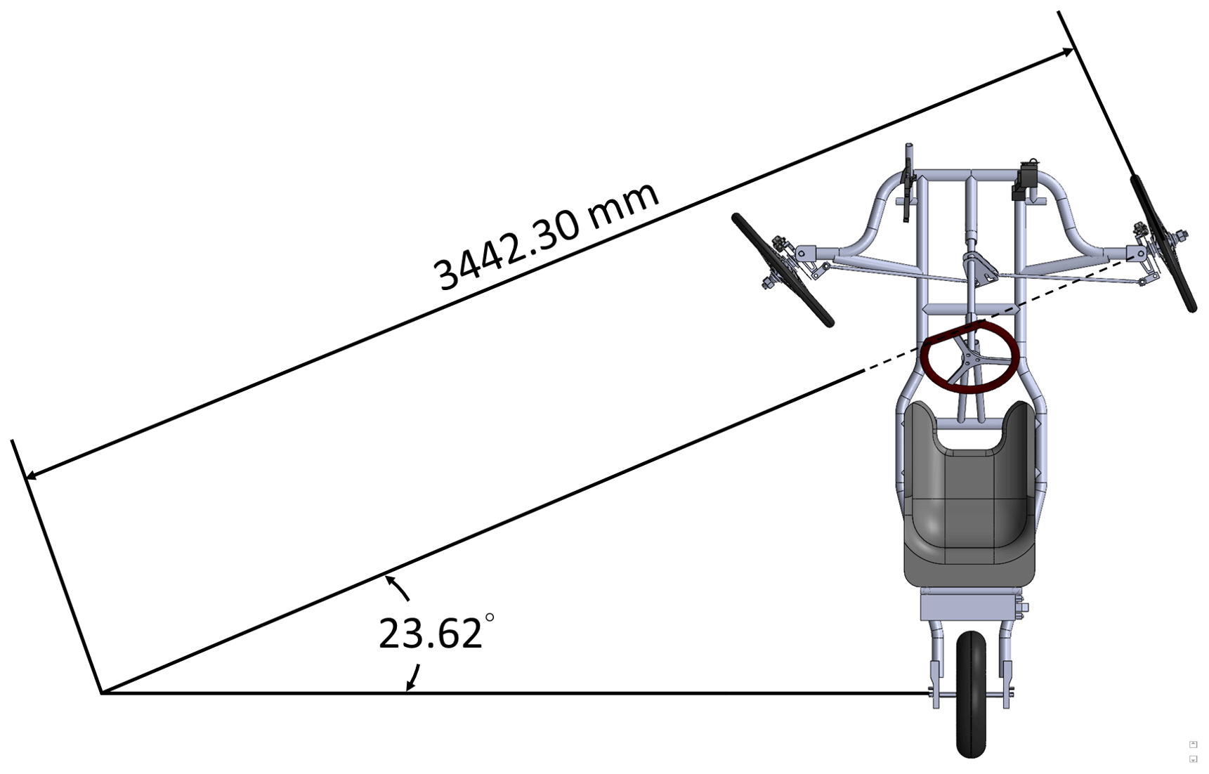
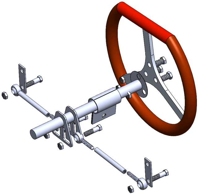
The system steering geometry is the main factor considered in the steering design. According to the vehicle running speed and racing track condition, the steering design used positive Ackermann steering to implement low-speed curves, and the wheel path corresponding to the theoretical turning radius in the cornering of the vehicle is calculated. As the designed turning radius (RS=3.44 m) is smaller than the curve in the competition area (RL=6.0 m), the vehicle can complete in passing this curve, as shown in Fig. 6. An exploded view of the steering system is shown in Fig. 7.
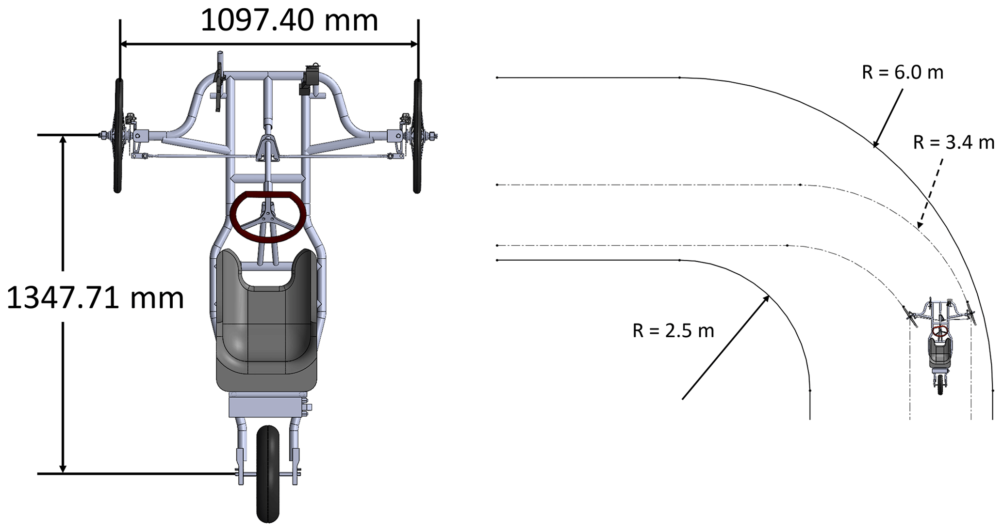
Figure 6Schematic diagrams of the Ackermann steering geometry (positive Ackermann) and the wheel path.
3.3 Front and rear axle load parameter analysis
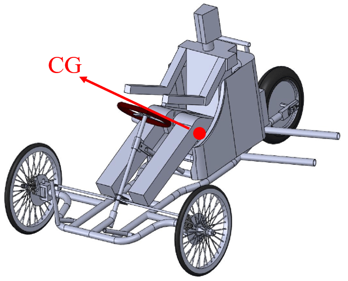
The center of gravity of the vehicle is defined as the position of the center of mass; thus, the individual centroid position of each object on the vehicle is determined, and then the weights on the front and rear axles are worked out respectively, as shown in Fig. 8.
3.3.1 Static state
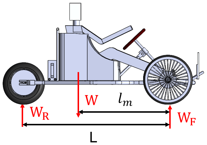
According to the static load equation (Seward, 2014), the rear wheel load WR could be expressed as follows:
where, W is the full-vehicle weight, lm is the wheel base from the center of gravity position of the vehicle to the front wheel, and L is the axial length from the rear wheel to front wheel. The front wheel load WF could be expressed as follows:
The distance from the center of gravity to the front and rear wheel center is worked out, as shown in Fig. 9. The substitution parameter is obtained by Eqs. (6) and (7) to obtain the static load state, in which W=1774.3347 N, lm=0.83 m, L=1.34 m, WR=1095.64 N, and WF=678.68 N.


3.3.2 Acceleration
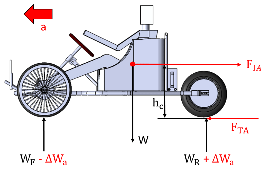
When the vehicle is in motion, the inertia force FIA generated by acceleration would change the stress on the parts, and the rear wheel axle part would bear the maximum load, as shown in Fig. 10. Therefore, the traction force FTA generated by the acceleration of the vehicle is (Seward, 2014) as follows:
where, μs is the tire friction coefficient, hC is the height of the center of gravity to the ground, and FTA is the traction force induced by acceleration. To obtain the maximum load on the rear wheel axle part during acceleration, the weight transfer during vehicle acceleration is (Seward, 2014) as follows:
where μs=1.35 and hC=0.30, FTA=2119.25 N, and ΔWa=474.10 N for the case of the designed frame structure.
3.3.3 Braking
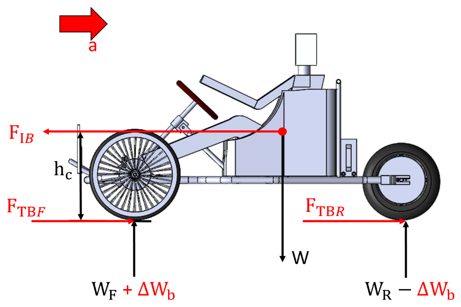
According to the aforementioned concept, when the vehicle is braking, the front wheel axle part would bear the maximum load, as shown in Fig. 11. The traction force FTB will be equal to the inertial force FIB generated at this time. Therefore, the traction force FTB generated when the vehicle is braking is (Seward, 2014) as follows:
To obtain the maximum load on the front wheel axle part during braking, the weight transfer during braking is obtained (Seward, 2014) as follows:
FTB=2395.35 N and ΔWb=535.87 N after calculation, and the deceleration during braking is derived from FTB=2395.35 N and m=180.87 kg.
3.3.4 Cornering
To prevent the vehicle from overturning when cornering, the object centroid position is analyzed first, and the right and left distances from the center of gravity to the front wheels are worked out, as shown in Fig. 12. The maximum cornering force FTc generated during the cornering of the overall vehicle is established on the rare skid of tires; therefore, the cornering force FTc will be equal to the centrifugal force of the vehicle. The total transverse weight transfer is (Seward, 2014) as follows:
where FTc of the vehicle can be expressed as follows:
In the design, the target working condition is at a speed of 40 km h−1 so that it can pass through the 71.31 m curve in the track. The parameter LF=950 mm and the calculated FTc=331.13 N are substituted into it, and ΔWc=98.88 N is obtained. It can be seen that, when the vehicle is not suspended, it can cope with the planned working conditions, so the shock absorber is removed to reduce the weight of the vehicle.
3.4 Part stress analysis
Finite element analysis is used to combine the calculation result with the free body diagram for stress analysis. The stress distribution trend and the position of maximum stress are observed to ensure sure that the received stress would not exceed the yield strength to induce plastic deformation. SS400 low carbon steel, with the same carbon dosage as the frame tube, is used to avoid cold cracking during welding. The material parameters of the designed car parts are listed in Table 7.

3.4.1 Front wheel steering knuckle
The caliper locking point received the maximum pull during braking, and the knuckle pin hole site is given boundary conditions, as shown in Fig. 13. The front wheel assembly free body diagram and the pressure in the direction of the knuckle locking point position, shown in Eq. (9), are used for analysis, as shown in Fig. 14.
where f is the friction of the brake pad to the disc, ri is the effective radius from the wheel center to the brake pad, (WF+Wb)μs is the friction of the tire to the ground during braking, and ro is the tire radius.
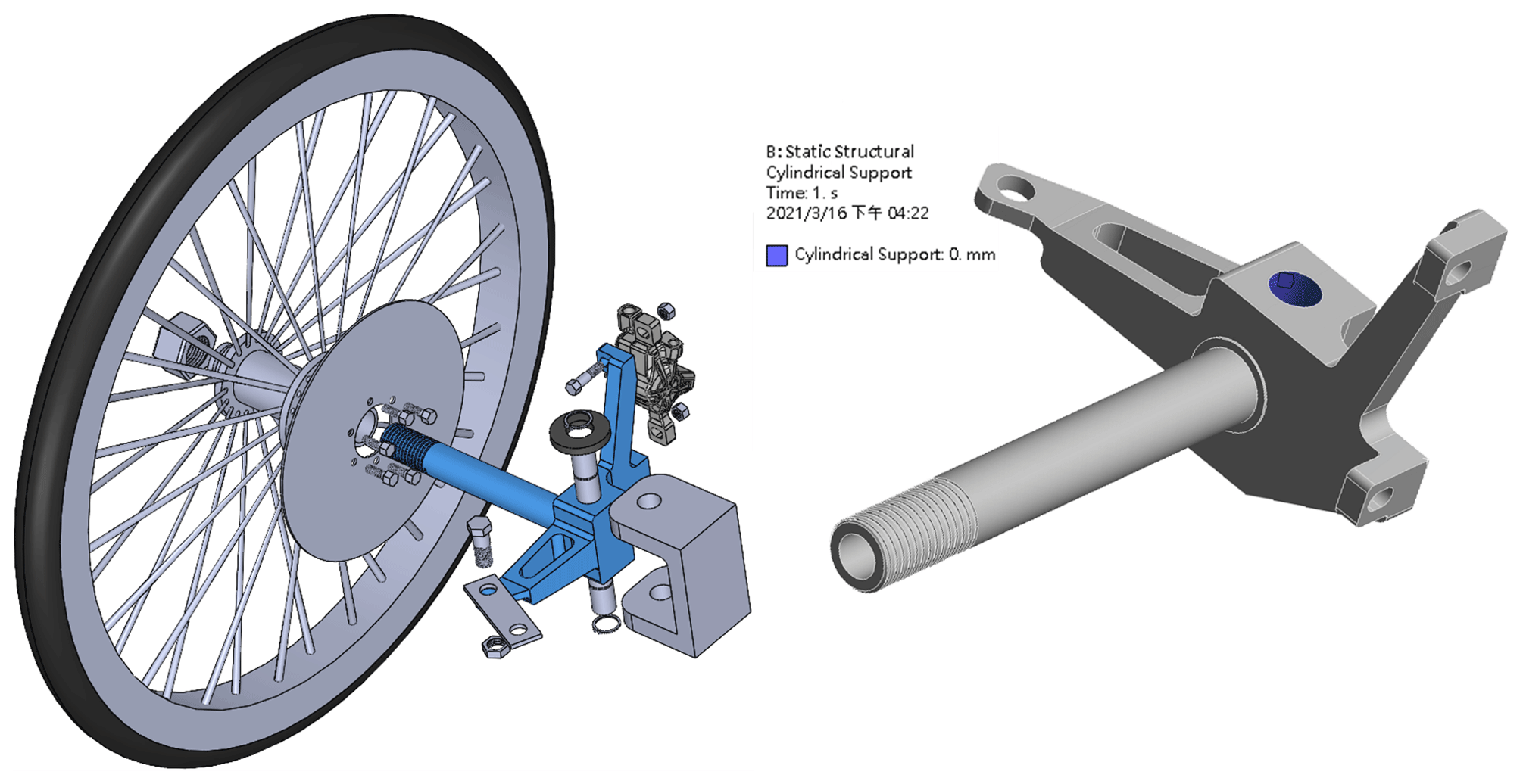
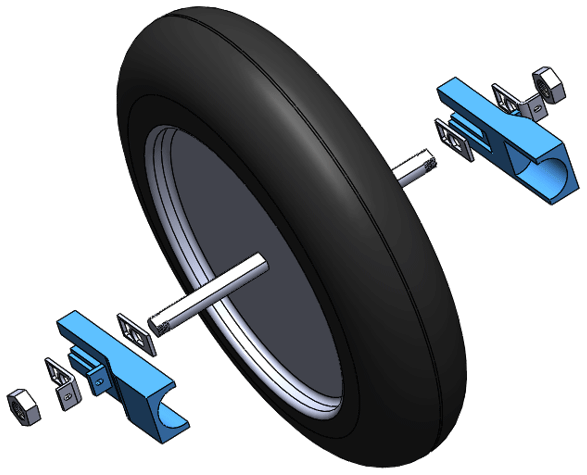
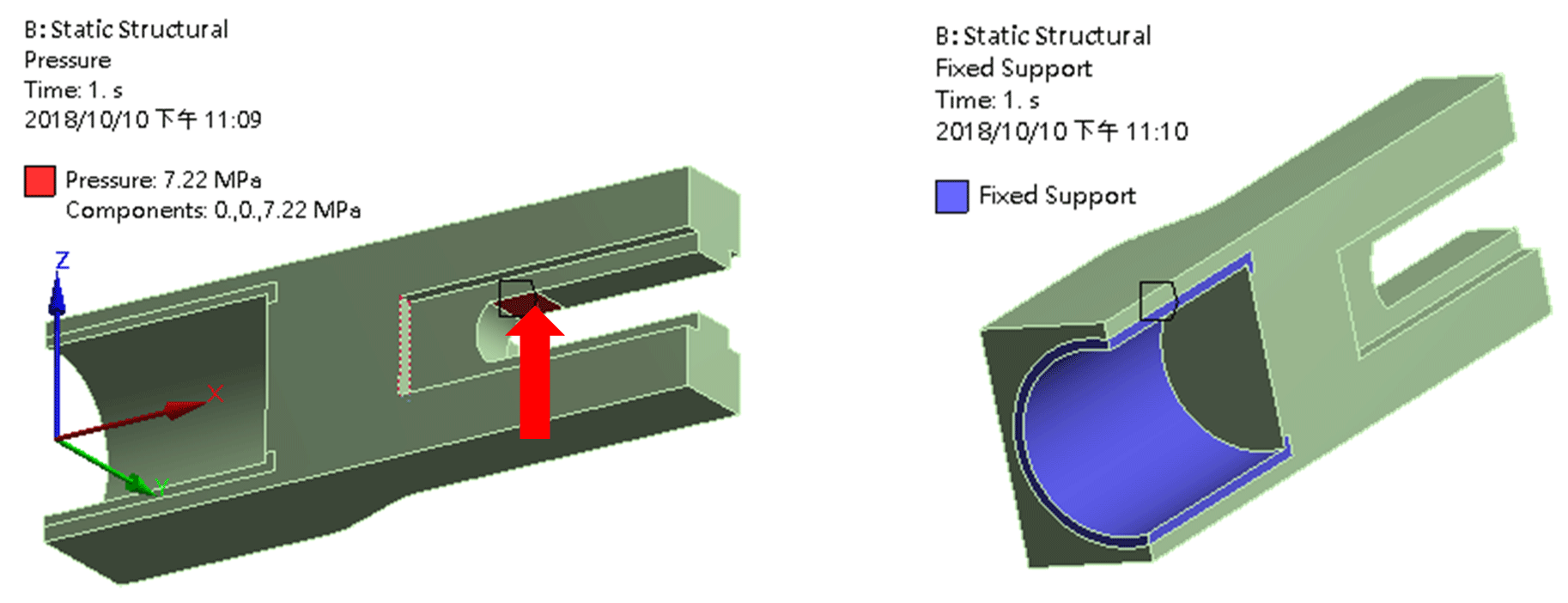
3.4.2 Rear wheel axle fastener
The exploded view of the rear wheel assembly is shown in Fig. 15. When the vehicle is accelerating, the rear wheel axle fastener would bear the maximum load; it is joined to the frame by welding, so the contact with the frame beam is complete contraction, and the effective area of the axle connection is a given load, as shown in Fig. 16.
3.5 Frame rigidity analysis
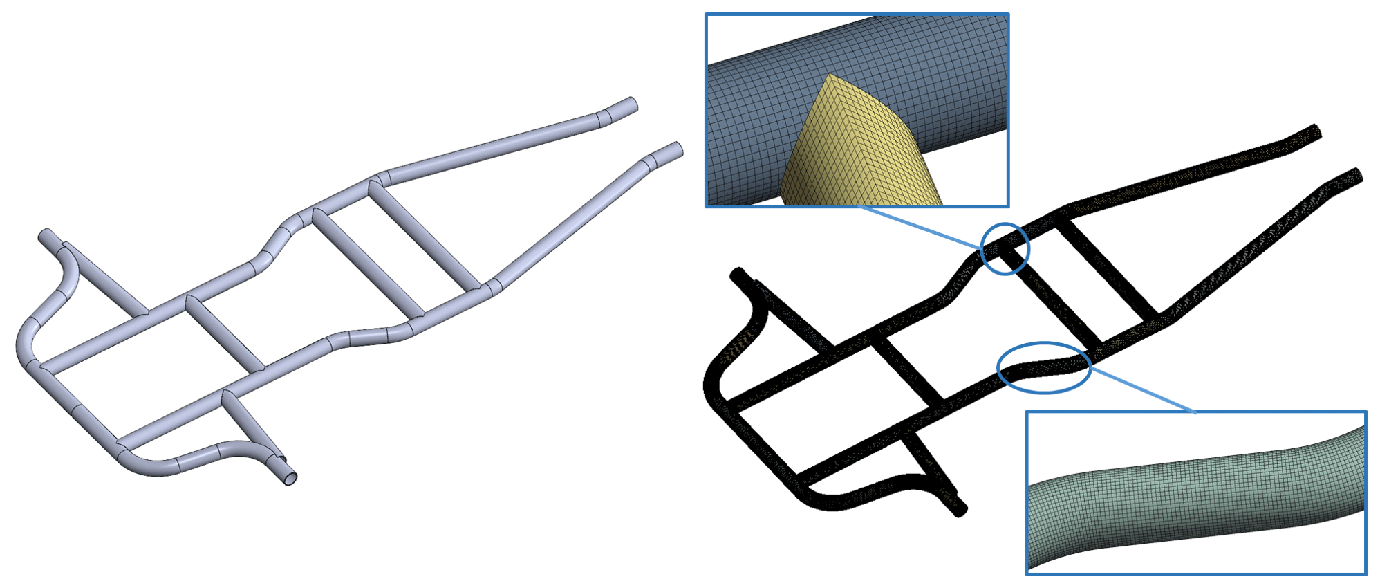
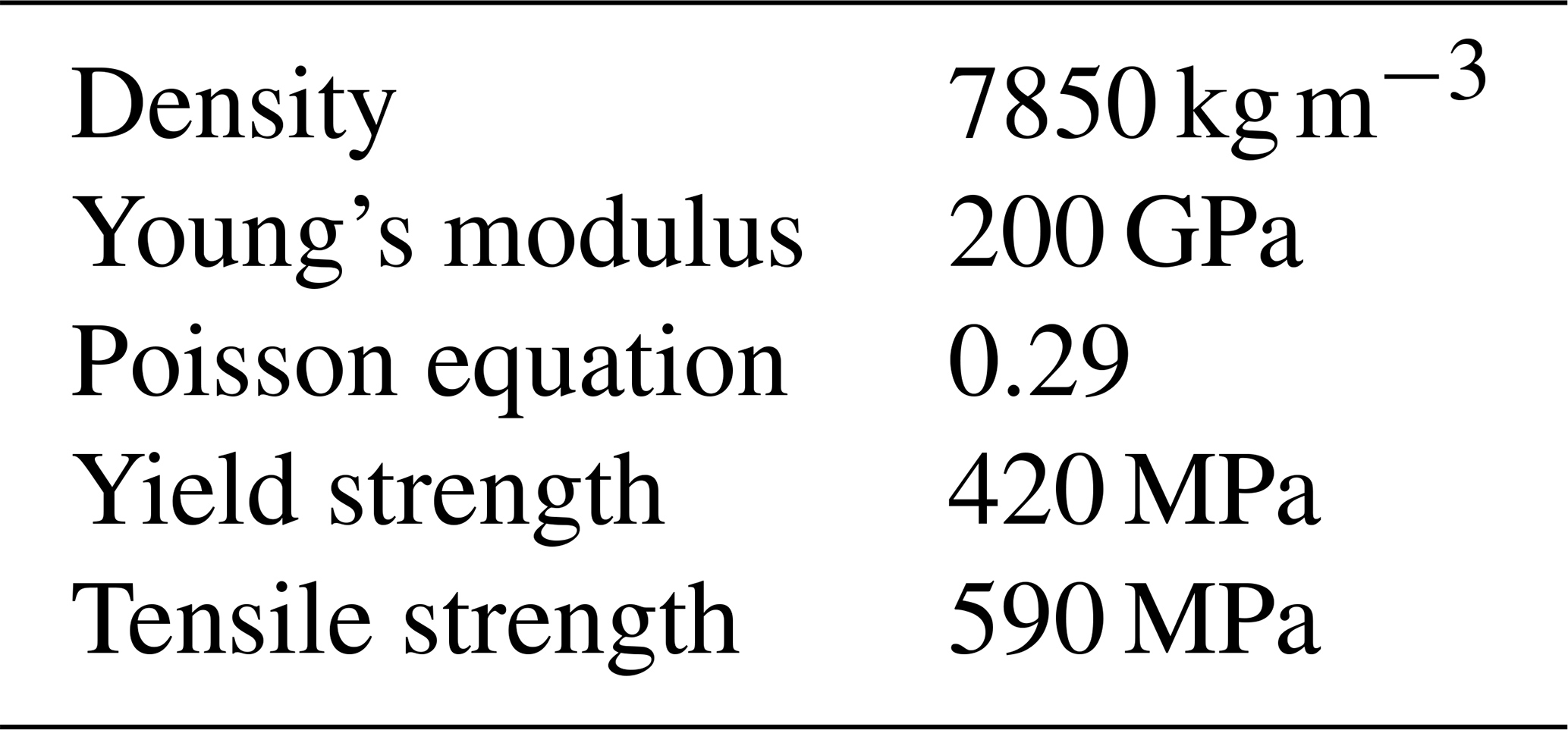
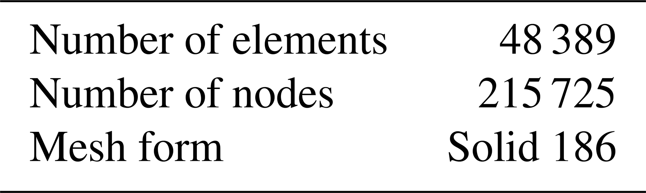
Rigidity refers to the resistance to the deformation of an object (Barton and Fieldhouse, 2018). This analysis discussed whether the frame rigidity could be enhanced effectively after stiffeners are applied (Curti, 1997). Our frame is welded and free of a suspension design, and the tube is made of SPFH590 (low carbon steel). The schematic diagram of the frame model and finite element model is shown in Fig. 17. The material parameters of SPFH590 and the finite element model parameters of the frame are, respectively, listed in Tables 8 and 9. In comparison to medium carbon steel and high carbon steel, low carbon steel has better elongation and weldability.
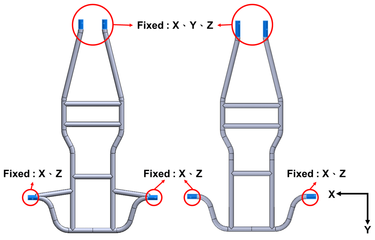
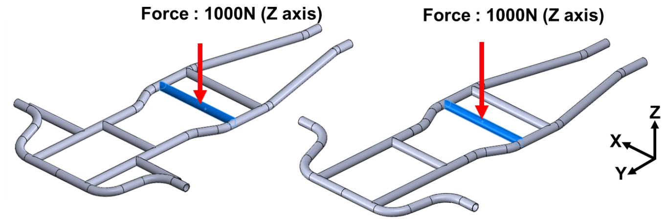
3.5.1 Bending rigidity
The bending rigidity is an index for evaluating the structural performance of a vehicle body. The three wheels supporting the vehicle body are restrained, and the vehicle load is applied to the vehicle centroid. The vertical power induced by acceleration and deceleration would increase the vertical deformation and increase deformation of the chassis (Mahmoodi-Kaleibar et al., 2014). For vehicles with a longer wheel base, the bending rigidity of the frame requires closer attention. According to the definition of bending rigidity (Milliken, 1994), load force F is given to the center of gravity of the frame, and the axle position is restrained during simulation, as shown in Figs. 18 and 19, and maximum displacement D is obtained. The relation could be expressed as follows:
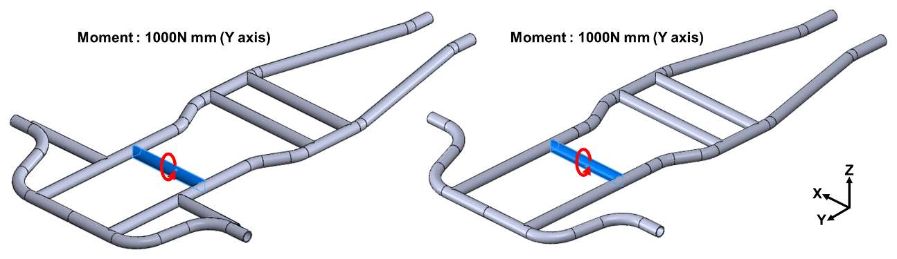
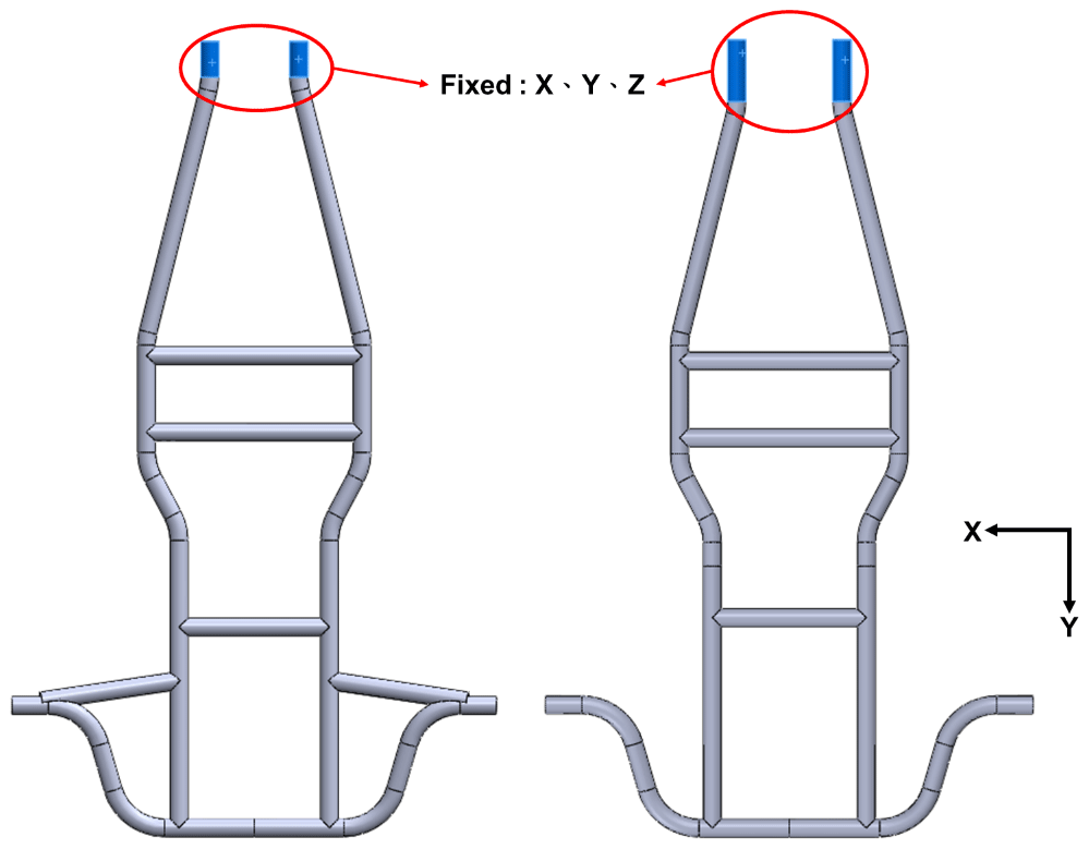
3.5.2 Torsional rigidity
Torsional rigidity (Parlaktaş et al., 2019; Tanik and Parlakta, 2015) refers to the resistance of the vehicle body structure to torsional deformation when the vehicle is cornering or running on a rough road, and it is an important index of road surface adaptability (Pourasad et al., 2016). Torsional rigidity is also one of the factors in handling performance of a vehicle. According to the definition of torsional rigidity (Milliken, 1994), the frame is given torque T at the steering column end, and the rear wheel axle position is restrained, as shown in Figs. 20 and 21. The frame generated an angle of torsion θ. The relation of torsional rigidity KT to torque T and the angle of torsion θ could be expressed as follows:
3.6 Modal analysis
The modal analysis is based on the finite element method. The analysis obtained the modal parameters of the system under the free boundary condition (Mishra and Sahu, 2012), including the modal frequencies and vibration mode shapes to know the dynamic characteristics of the system. The finite element method is used for the theoretical modal analysis of the built frame model, and the modal frequencies and corresponding vibration mode shapes of the model are obtained. The simple harmonic response analysis obtained the frequency response function between the simple harmonic external force input signal and the system output to obtain the sizes and phases of various measuring points for subsequent verification. The process is shown in Fig. 22.
3.7 Experimental modal analysis
The vibration mode shape corresponding to each modal frequency could be obtained by modal analysis; the actuation of the mode is observed, and the measuring points are planned as the basis of the experimental modal analysis (Orlowitz and Brandt, 2017).
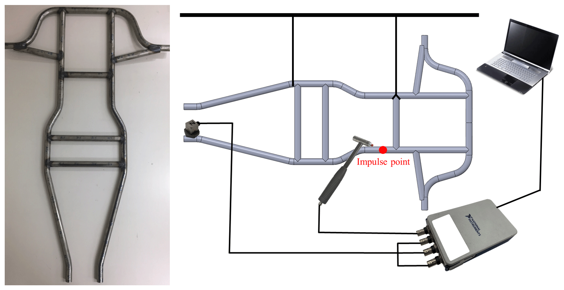
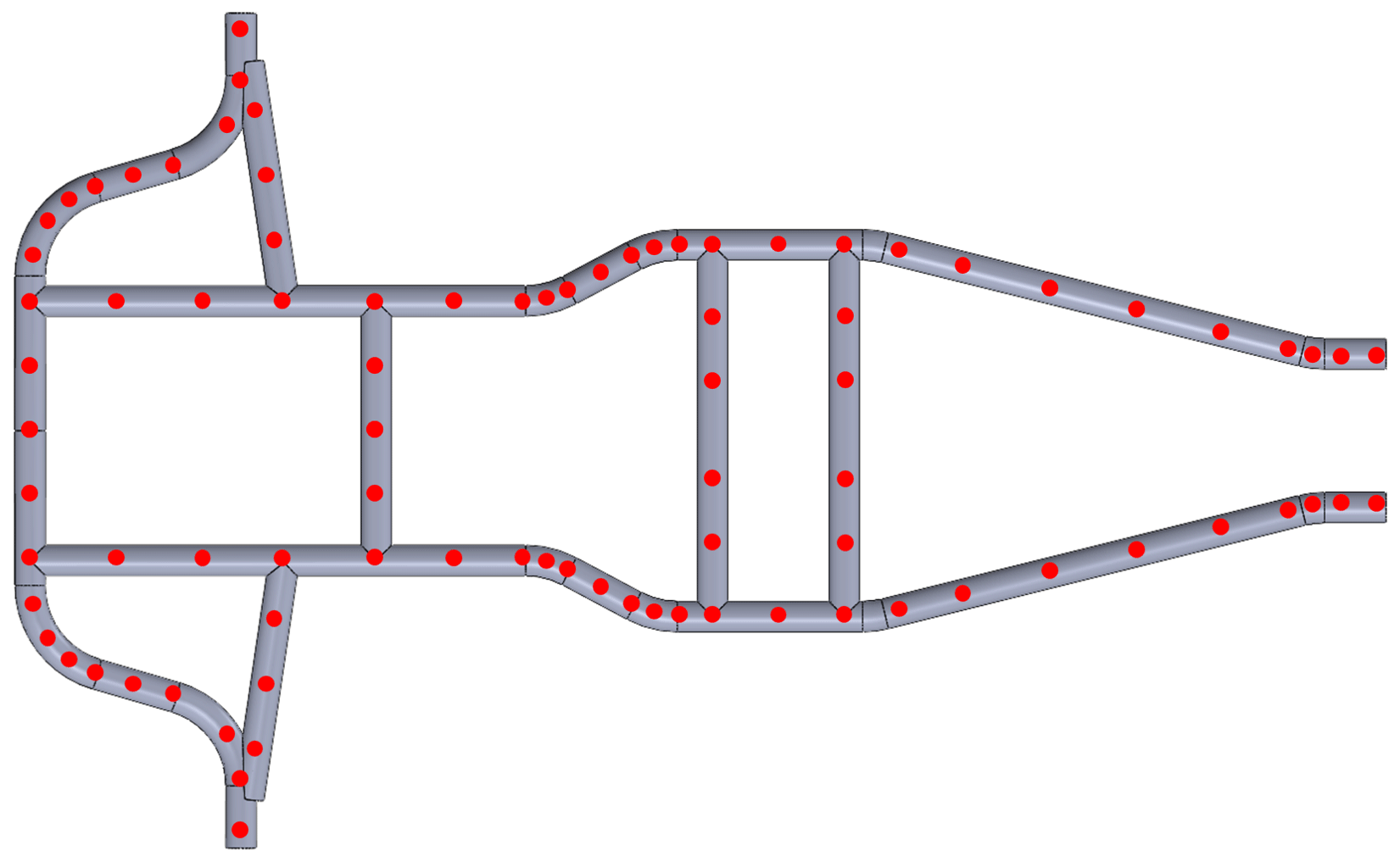
The experimental modal analysis aimed to identify the dynamic characteristics of unknown practical frame structures. The schematic diagram of the frame structure entity and experiment is shown in Fig. 23. In the experimental process, appropriate measuring points are spread over the practical frame structure, as shown in Fig. 24. An accelerometer is affixed to the frame structure, and an impact hammer is used to knock the actual structure and give it an excitation signal. The accelerometer obtained a response signal, and the excitation and response signals are processed by fast Fourier transform to obtain the frequency response function. The software then performed curve fitting to extract the modal parameters to determine the dynamic characteristics of the frame structure.
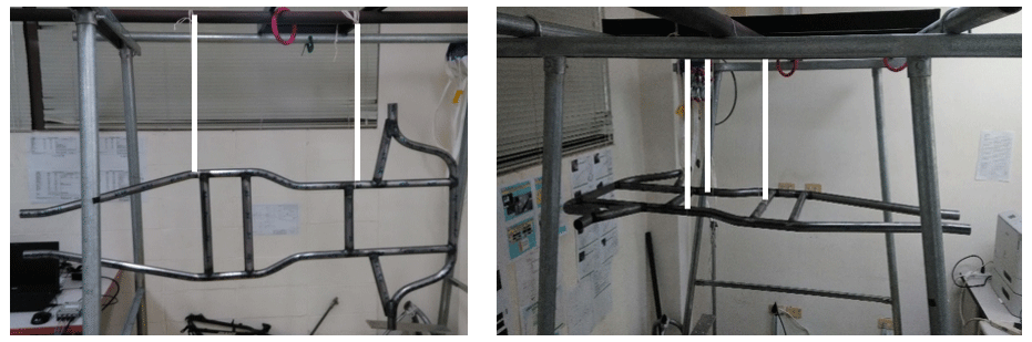
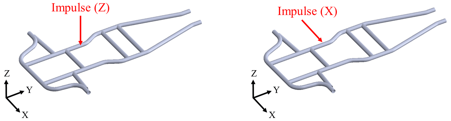
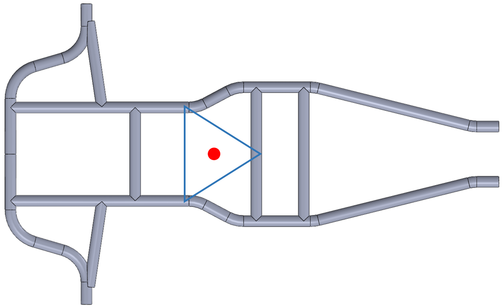
The vertical suspension frame structure is first excited by an impact hammer, as shown in Fig. 25. The z-axis excitation is applied by the impact hammer to the application point, as shown in Fig. 25, and the point of vertical suspension is the result of finite element analysis. A node is selected as the suspension point. The suspension method is changed according to the result of the suspension method. This method is based on a horizontal suspension frame structure, as shown in Fig. 26. The x-axis excitation is applied by the impact hammer to the application point, as shown in Fig. 26. In terms of the selection of the suspension points on the horizontal suspension frame structure, an equilateral triangle is drawn at the center of gravity, and the three endpoints of the triangle become the suspension points, as shown in Fig. 27.
3.8 Modal assurance criterion (MAC)
The modal assurance criterion (MAC; Allemang and Brown, 1983) is used to verify the consistency of the mode shapes ΦiA and ΦjX obtained, respectively, from finite element analysis (FEA) and experimental modal analysis (EMA) of the frame. The definition of the MAC is as follows:
where T and ∗ denote, respectively, the transpose and complex conjugate of a matrix or vector. When the MAC value approached 1.0, the two vectors ΦiA and ΦjX represented approximately the same mode shape. On the contrary, when the MAC value approached 0.0, the two mode shapes were orthogonal with each other.
4.1 Axle part stress analysis
As the result of a single analysis would be unreliable, the precision of the analysis needed to be guaranteed by convergence analysis. The result trend is judged according to the refined net, and a slope of two consecutive analysis results closer to zero would indicate the results are closer to convergence.
4.1.1 Front wheel steering knuckle
According to the analysis result, the maximum stress occurred in the upper locking point position, as shown in Fig. 28. The elements in the position are refined, and the convergence curve is as shown in Fig. 29.
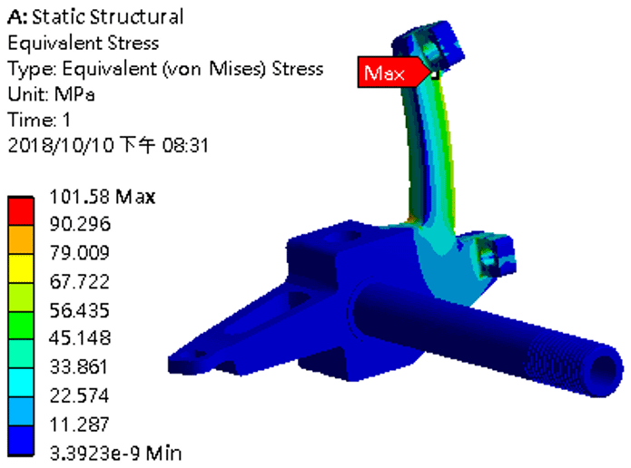

According to the analysis result, the line slope is lower than 0.1 after the locking point stress 101.33 MPa of the knuckle during braking. The analysis result showed that the stress is 101.58 MPa, lower than the 245 MPa yield strength of the material (Juvinall and Marshek, 2019).
4.1.2 Rear wheel axle fastener
According to the analysis result, the maximum stress occurred at the edge of the joint seat, as shown in Fig. 30. After the elements are refined, the convergence curve is as shown in Fig. 31.
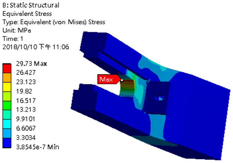
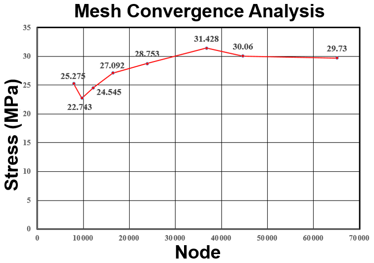
The line slope is lower than 0.1 after the stress of 30.060 MPa at the junction of the rear axle part with the axle during acceleration. The analysis result showed that the stress is 29.730 MPa, lower than the 225 MPa yield strength of the material (Juvinall and Marshek, 2019).
4.2 Rigidity result comparison
4.2.1 Bending rigidity
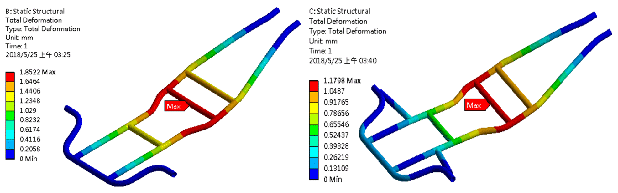
The analysis result in Fig. 32 shows that the bending rigidity (Mohseni Kabir et al., 2017) of the frame without stiffeners is , and that the bending rigidity of the frame with stiffeners is , indicating an increase of 83.50 %. When the chassis structure is under a bending load, the displacement should not be larger than 1 mm (Dzerkelis et al., 2012). After deducting the weight of the hub motor and front wheel, the force at the center of gravity of the full vehicle is 890.53 N, and the force induces a 0.88 mm displacement at the center of gravity of the structure.
Table 10The verification results of modal assurance criterion (MAC) for the mode shapes obtained from the experimental modal analysis (EMA) and finite element analysis (FEA) of the frame.
4.2.2 Torsional rigidity
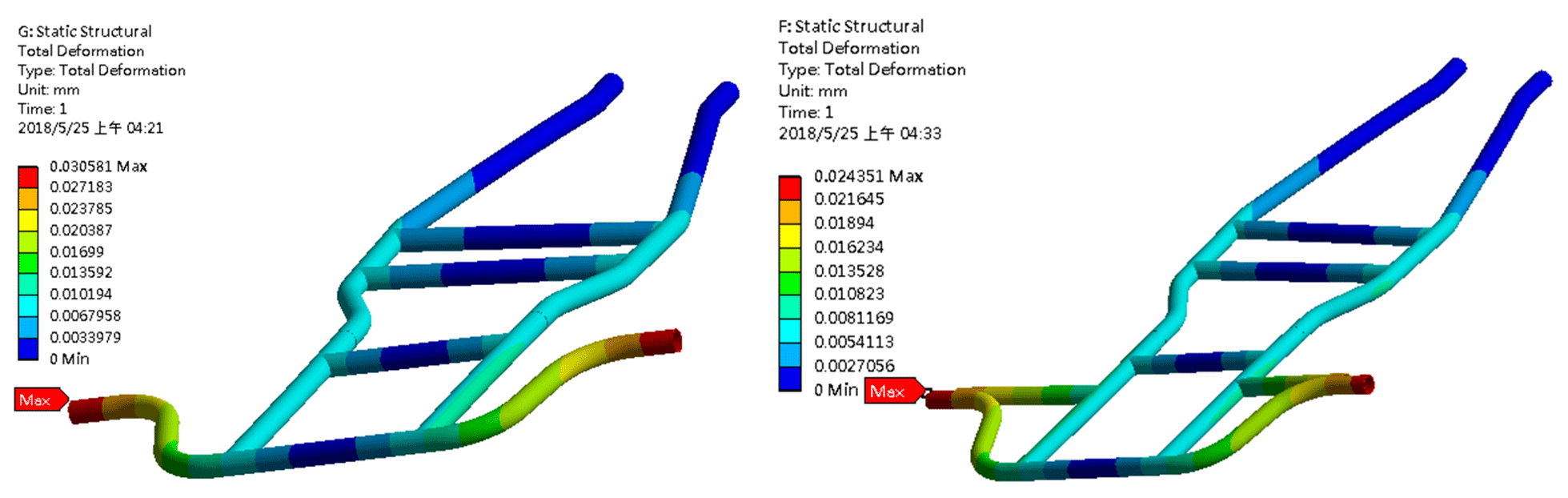
The analysis result in Fig. 33 shows that the torsional rigidity (Mohseni Kabir et al., 2017) of the frame without stiffeners is , and that the torsional rigidity of the frame with stiffeners is , indicating an increase of about 27.59 % after reinforcement.
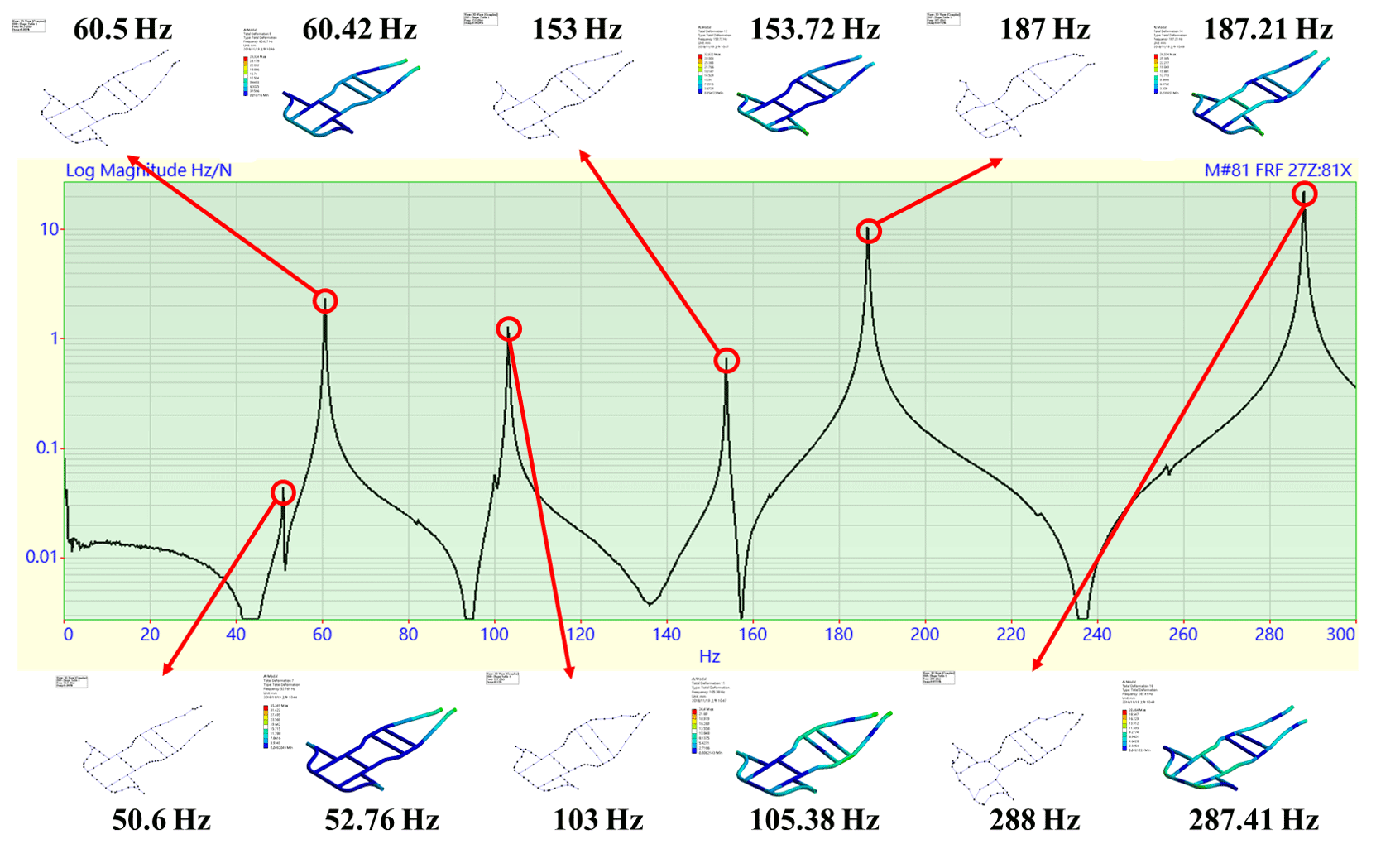
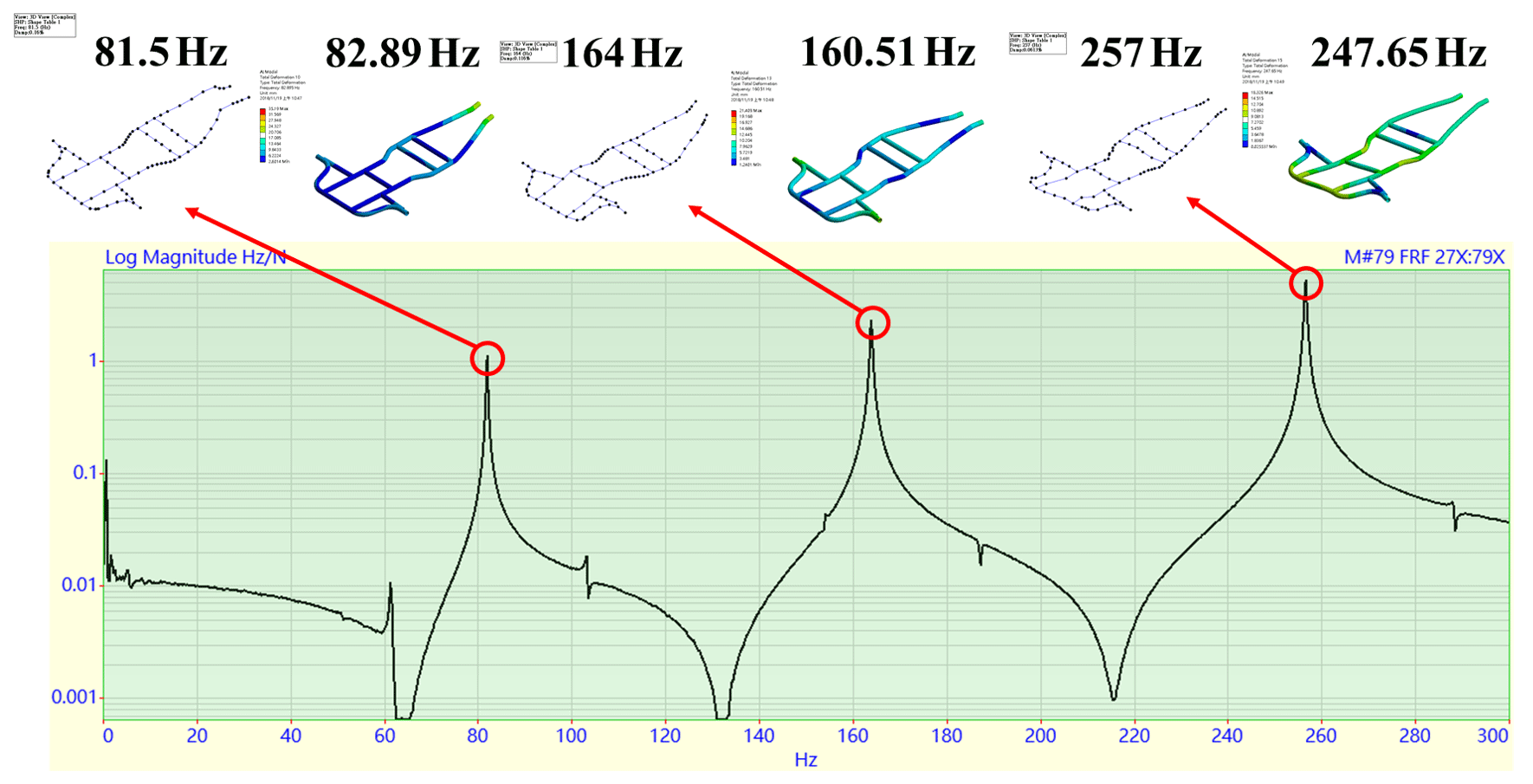
4.3 Comparison between finite element analysis and experimental modal analysis results of the frame
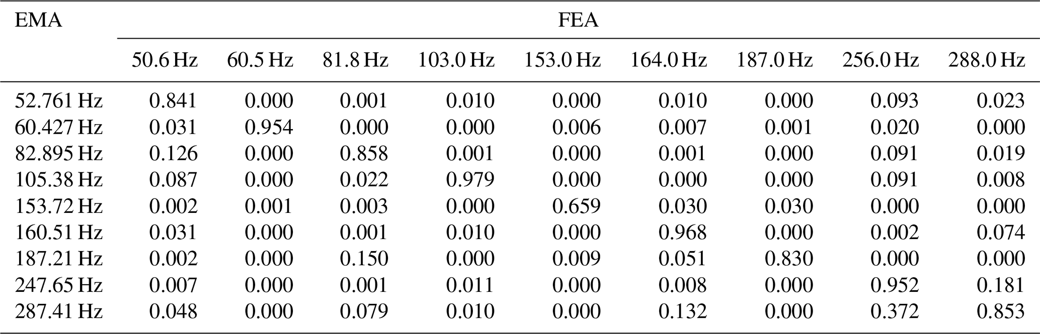
To guarantee the equivalence of the finite element model of the frame, the results of the finite element analysis and the experimental modal analysis of the frame are compared (Li and Feng, 2020). Figure 34 shows that there are six peaks, while Fig. 35 shows three peaks. The peaks had corresponding modal frequencies and vibration mode shapes, as shown in Table 10. There is a slight difference in the vibration mode shapes, according to a visual inspection, and according to the result comparison, the frequency errors of different modes in the finite element analysis and experimental modal analysis are less than ±5 %.
4.4 MAC
According to Table 10 and Fig. 36, the corresponding modes have higher index values and are generally symmetric. As the fifth mode had a bending mode and bouncing mode at the same time, the mode comparison required more mode information, and the index value of the mode is relatively low.
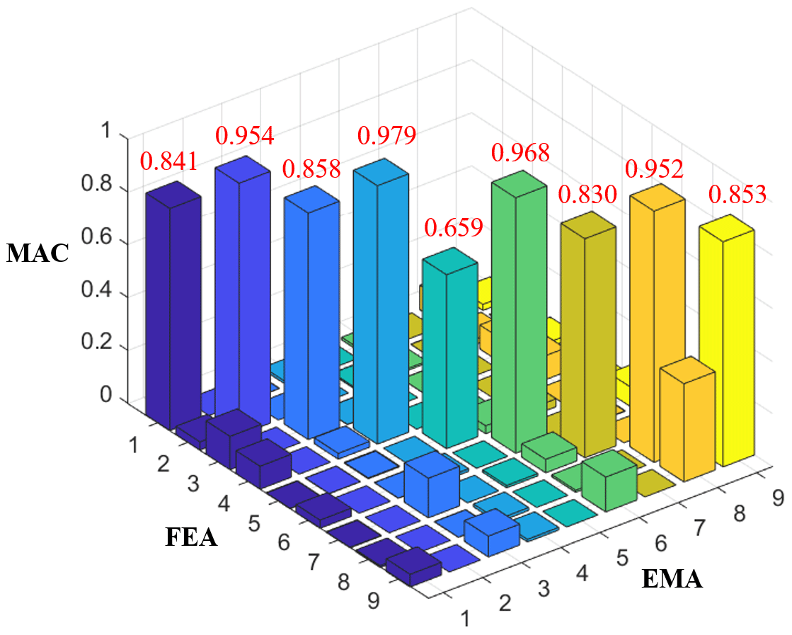
Figure 36Typical plot of the modal assurance criterion (MAC) for the mode shapes obtained from the experimental modal analysis (EMA) and finite element analysis (FEA) of the frame.
In this vehicle design, in order to obtain excellent performance, the model validity is verified by the finite element method and experimental modal analysis. The conclusions are as follows:
-
For the designed frame of this vehicle, the geometric dimension of the minimum turning radius needed to meet the racing track condition is designed by steering geometry analysis, and the average front and rear wheel loads of the vehicle during braking are derived from the front and rear axle loading conditions.
-
As the front and rear axle part analysis results did not exceed the yield stress of the selected material, SS400, the parts did not suffer from plastic deformation during braking or acceleration.
-
According to the rigidity analysis, the bending rigidity and torsional rigidity are noticeably enhanced after the stiffeners are installed.
-
According to the definition of the frequency response function, in terms of the system resonance conditions, the system frequency needed to be consistent, and the vibration mode shapes and experimental excitation needed to be in the same phase. Therefore, the concept is imported into the frame design to confirm the consistency of the analytic mode and experimental mode.
All the code used in this paper can be obtained upon request to the corresponding author.
All the data used in this paper can be obtained upon request to the corresponding author.
CSL, CCY, and YHC conceived of the presented idea. We design the light electric vehicle and CHH performed the CAE. CSL, YHC and YXW verified the analytical methods and YTL supervised the findings of this work. All the authors discussed the results and contributed to the final manuscript.
The authors declare that they have no conflict of interest.
The authors would like to thank anonymous reviewers for their valuable comments and suggestions for revising the paper.
This research was supported in part by Ministry of Science and Technology of Taiwan (grant no. MOST 109-2221-E-020-001-).
This paper was edited by Engin Tanık and reviewed by Mehdi Mahmoudi-K and two anonymous referees.
Afkar, A., Mahmoodi-Kaleibar, M., and Paykani, A.: Geometry optimization of double wishbone suspension system via genetic algorithm for handling improvement, J. Vibroeng., 14, 827–837, 2012.
Allemang, R. J. and Brown, D. L.: A Correlation Coefficient for Modal Vector Analysis, Proceedings of the 1st International Modal Analysis Conference, Society for Experimental Mechanics, Bethel, 1983.
Barton, D. C. and Fieldhouse, D.: Vehicle Structures and Materials, Chapt. 4 in: Automotive Chassis Engineering, Springer, Cham, Switzerland, 2018.
Curtis, H. D.: Fundamentals of Aircraft Structural Analysis, McGraw-Hill, USA, 1997.
Dzerkelis, V., Bazaras, Z., Sapragonas, J., and Lukoševičius, V.: Investigation of the Experimental Car Body in Static Bending and Torsion, Mechanika, 18, 392–397, 2012.
Juvinall, R. C. and Marshek, K. M.: Failure Theories, Safety Factors, and Reliability, Chapt. 6 in: Fundamentals of Machine Component Design, 7th edn., John Wiley & Sons, Inc., USA, 2019.
Kabir, M. M., Izanloo, M., and Khalkhali, A.: Concept design of Vehicle Structure for the purpose of computing torsional and bending stiffness, Int. J. Automot. Eng., 7, 2370–2377, https://doi.org/10.22068/ijae.7.2.2372, 2017.
Li, S. and Feng, X.: Study of structural optimization design on a certain vehicle body-in-white based on static performance and modal analysis, Mech. Syst. Signal Process., 135, 106405, https://doi.org/10.1016/j.ymssp.2019.106405, 2020.
Mahmoodi-Kaleibar, M., Davoodabadi, I., Višnjić, V., and Afkar, A.: STRESS AND DYNAMIC ANALYSIS OF OPTIMIZED TRAILER CHASSIS, Tehnicki Vjesnik, 21, 599–608, 2014.
Marzbanrad, J., Soleimani, G., Mahmoodi-Kaleibar, M., and Rabiee, A. H.: Development of fuzzy anti-roll bar controller for improving vehicle stability, J. Vibroeng., 17, 3856–3864, 2015.
Milliken, W.: SAE international, Wheel Loads, Chapt. 18, in: Race Car Vehicle Dynamics, SAE International, USA, 1994.
Mishra, I. and Sahu, S. K.: An Experimental Approach to Free Vibration Response of Woven Fiber Composite Plates under Free-Free Boundary Condition, Int. J. Adv. Technol. Civ. Eng., 1, 148–153, 2012.
Orlowitz, E. and Brandt, A.: Comparison of Experimental and Operational Modal Analysis on A Laboratory Test Plate, Measurement, 102, 121–130, https://doi.org/10.1016/j.measurement.2017.02.001, 2017.
Parlaktaş, V., Tanık, E., Babaarslan, N., and Çalık, G.: The Design and Manufacturing Process of an Electric Sport Car (EVT S1) Chassis, Iran. J. Sci. Technol., T. Mech. Eng., 45, 103–113, https://doi.org/10.1007/s40997-019-00328-6, 2019.
Pourasad, Y., Mahmoodi-Kaleibar, M., and Oveisi, M.: Design of an optimal active stabilizer mechanism for enhancing vehicle rolling resistance, J. Central South Univ., 23, 1142–1151, 2016.
Seward, D.: Racing car basics, Chapt. 1 in: Race Car Design, MacMillan Education, UK, 2014.
Tanık, E. and Parlaktaş, V.: Design of a very light L7e electric vehicle prototype, Int. J. Automot. Tech., 16, 997–1005, 2015.