the Creative Commons Attribution 4.0 License.
the Creative Commons Attribution 4.0 License.
 | 25 Feb 2021
A real-time inverse kinematics solution based on joint perturbation for redundant manipulators
Qinhuan Xu
Qiang Zhan
Aiming at the problem that the calculation of the inverse kinematics solution of redundant manipulators is very time-consuming, this paper presents a real-time method based on joint perturbation and joint motion priority. The method first seeks the pose nearest to the target pose in the manipulator's pose set through fine-tuning all the joints with different angle deviations at the same time and then regards this pose as the starting one to perform iterative calculations until the error between the current pose and the target pose is less than the predetermined error, thus obtaining the inverse kinematics solution corresponding to the target pose. This method can avoid the pseudo-inverse calculations of the Jacobian matrix and significantly reduce the solving complexity. Two types of manipulators are taken as examples to validate the proposed method. Under the premise that the manipulator motion trajectory is satisfied, the Jacobian pseudo-inverse method and the proposed method are both adopted to solve the inverse kinematics. Simulations and comparisons show that the proposed method has better real-time performance, and the joint motions can be flexibly controlled by setting different joint motion priorities. This method can make the work cycle faster and improve the production efficiency of redundant manipulators in real applications.
- Article
(7153 KB) - Full-text XML
- BibTeX
- EndNote


Until the present, in the manufacturing industry, traditional industrial manipulators with 6 or fewer degrees of freedom (DOFs) have been widely used in such tasks as transporting, assembling, spraying, and welding. However, with the diversification of production environments and task requirements, manipulators are required to have more flexible motions and obstacle avoidance capability. Therefore, manipulators with redundant DOFs have gradually attracted people's favour for higher flexibility and adaptability compared to traditional manipulators (Aouache et al., 2019; Akbaripour and Masehian, 2017; Omrcen and Zlajpah, 2007). The additional DOFs have led to redundant manipulators being able to complete tasks such as obstacle avoidance, joint limit avoidance, and load distribution optimization while performing specific production tasks (Liu et al., 2017), such as welding and polishing. To speed up the work cycle and improve production efficiency, higher requirements are imposed on the real-time performance of manipulators (Kalra et al., 2006; Kuhlemann et al., 2016). Compared to non-redundant manipulators, redundant manipulators have null space, and thus the inverse kinematics solution is not unique, and the process is more complicated and time-consuming. As a bottleneck problem of motion control and path planning, the high real-time inverse kinematics solution of redundant manipulators has caused much concern (Dasgupta et al., 2009; Kouabon et al., 2020).
Until the present, numerous research studies have focused on the inverse kinematics solution of redundant manipulators, and the methods can be divided into three types: geometric methods, numerical methods, and iterative methods (Jia et al., 2014). Transforming the inverse kinematics problem into a geometric one in a two-dimensional plane or a three-dimensional space, geometric methods (Tian et al., 2020; Faria et al., 2018; Zaplana et al., 2018) are suitable for redundant manipulators with a simple structure or special structure. Numerical methods include the Jacobian pseudo-inverse method (Hayashibe et al., 2006; Park et al., 2018), the gradient projection method (Zu et al., 2005), the generalized Jacobian method (Kumar et al., 2010), and the weighted minimum norm method (Maciejewski and Klein, 1985; Mohamed et al., 2009). However, these methods usually make equivalent approximations to the kinematics models of redundant manipulators during the solving process, inevitably leading to error accumulation. The high non-linearity and complex coupling of redundant manipulators have also resulted in the use of iterative algorithms to obtain inverse kinematics solutions. Korein and Badler (1982) first proposed the use of the iterative method to calculate the inverse kinematics solution of redundant manipulators. The limitation of this kind of method, however, is that the convergence of the solving results depends on the setting of the initial pose. Damas (2012) proposed an algorithm that can learn the input–output relationship of kinematics online and is suitable for solving forward and inverse kinematics of manipulators. Ayusawa and Nakamura (2012) proposed a fast inverse kinematics method that calculates the gradient vector with the Newton–Euler iterative algorithm to obtain the inverse solution. In addition, some methods based on genetic algorithms (Zeng et al., 2018), neural networks (Xia and Wang, 2001), particle swarm optimization (PSO) (Umar et al., 2019), and differential evolution (DE) (Lopezfranco et al., 2018) can also solve the inverse kinematics problem of redundant manipulators in an iterative manner. However, these iterative algorithms require extensive calculations and are very time-consuming.
The inverse kinematics algorithms of redundant manipulators are mainly evaluated from indexes such as real-time, reliability, stability, and universality (Tolani et al., 2000). The geometric method is fast and accurate for solving inverse kinematics, but it depends on the specific structure and geometric characteristics of manipulators and lacks universality. The numerical method and iterative method have the advantages of strong universality as they can be applied to hyper-redundant manipulators as well as constraints and objective functions in optimization problems, but they are not suitable for online real-time path planning because of extensive calculations, poor real-time performance, and low precision.
This paper presents a real-time method based on joint perturbation to obtain the inverse kinematics solution of redundant manipulators, which has no constraints on the DOFs, sizes, and structures of redundant manipulators. The remainder of this paper is organized as follows. In Sect. 2, the inverse kinematics method based on joint perturbation is introduced. In Sect. 3, simulations and comparisons are provided to validate the proposed method. Finally, conclusions of the paper are given in Sect. 4.
2.1 Kinematics model of redundant manipulators
If the dimension of a manipulator's work space is m, and the dimension of its joint space is n, when m<n, the manipulator has n−m redundant DOFs. The kinematics model of the redundant manipulator can be established with the modified D–H method (Denavit–Hartenberg; Lv and Liu, 2016). First, the D–H coordinate systems of all the links are established. The z axis of coordinate system {i} is collinear with the axis of joint i, which is located at the beginning of link i. The x axis coincides with the common perpendicular of joint i and joint i+1, pointing from joint i to joint i+1, and the y axis can be determined by the right-hand rule. The D–H transformation parameters are determined according to the relations of neighbouring frames, and then the homogeneous transformation matrix of frame {i} relative to frame {i−1} can be attained.
where ai−1 represents the length of the common perpendicular to the axes of joint i−1 and joint i, αi−1 represents the angle between the axes of joint i−1 and joint i, di−1 represents the offset of link i relative to link i−1, and θi represents the rotation angle of link i relative to link i−1 around the axis of joint i. Multiplying all the homogeneous transformation matrices in order results in the forward kinematics model of the manipulator.
Define as the joint variables of the manipulator, and the pose of the manipulator is P=f(q). When the current joint angles of the manipulator are , the current pose of the manipulator P0 can be obtained by
The target pose of the manipulator Pt can be determined according to task requirements. The inverse kinematics solution of the manipulator is used to obtain the joint variables qt according to the initial pose P0 and the target pose Pt. A redundant manipulator with n DOFs has numerous inverse solutions, from which the optimal one should be selected in an actual motion control. This paper presents a real-time inverse kinematics method based on joint perturbation, in which two definitions including the joint motion priority and joint perturbation coefficient matrix are used.
2.2 Joint motion priority
First, define the motion priority of each joint as k1, k2, k3…kn−1, kn, . The larger the ki is, the higher the motion priority joint i has. When ki=0, the motion of joint i will be limited to zero. The priority of each joint can be determined according to task requirements. For example, when a manipulator's motion is planned based on energy optimization, according to the rule of “moving big joints less and small joints more”, the joint motion priorities can be set as . When a manipulator's motion is planned based on time minimization, the joint motion priorities can be set as to follow the rule of “moving big joints more and small joints less” (Xu et al., 2010). In particular, when a manipulator's motion is not constrained by tasks, the joint motion priorities can be set as so that all the joints have the same motion priority.
2.3 Joint perturbation coefficient matrix
Suppose the initial joint variables of a manipulator are , which correspond to the initial pose P0 of the manipulator. A very small angle δθ (δθ>0) is set as the basic perturbation angle, and the perturbation angle of joint i is Δθi. Thus, the perturbation angle of joint i is the product of the motion priority ki and the basic perturbation angle δθ.
A rotary joint has two types of possible motions: counter-clockwise or clockwise, so the coefficient of δθ can be 1 or −1. When the perturbation direction of joint i is counter-clockwise, Δθi=kiδθ; when the perturbation direction is clockwise, .
Hence, the perturbation variable Δq of a manipulator with n DOFs has 2n possible combinations. Each combination of the coefficients of the basic perturbation angle δθ of n joints constitutes a column vector, and all the column vectors constitute a matrix K, which is defined as the joint perturbation coefficient matrix. Figure 1 shows the joint perturbation combinations of three types of manipulators with 1 DOF, 2 DOFs, and 3 DOFs, and the construction of the joint perturbation coefficient matrix is introduced as follows.
When n=1, the manipulator has only 1 DOF and two types of possible motions, as shown in Fig. 1a. Therefore, the joint perturbation coefficient matrix of the manipulator is
When n=2, the manipulator has 2 DOFs and four types of possible motions, as shown in Fig. 1b, and the joint perturbation coefficient matrix is
When n=3, the manipulator has 3 DOFs and eight types of possible motions, as shown in Fig. 1c, and the joint perturbation coefficient matrix is
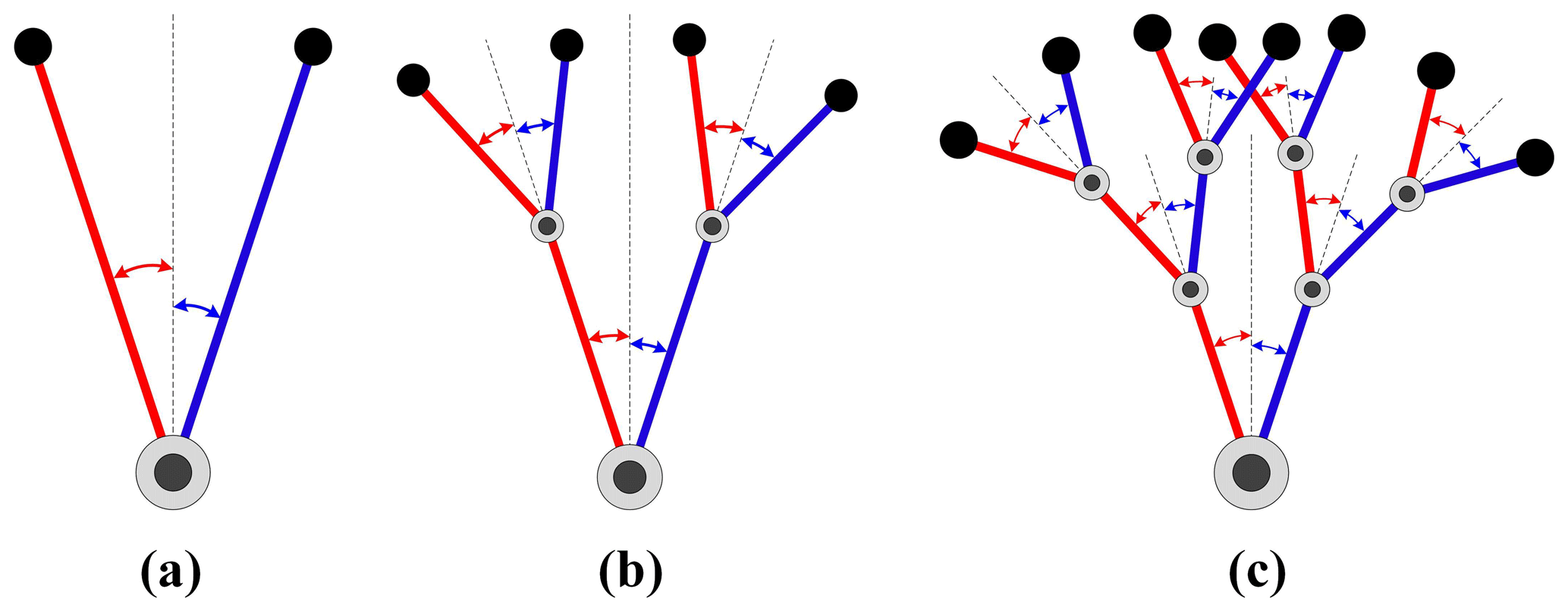
Figure 1Joint perturbation combinations of manipulator with n DOFs. (a) n=1. (b) n=2. (c) n=3.
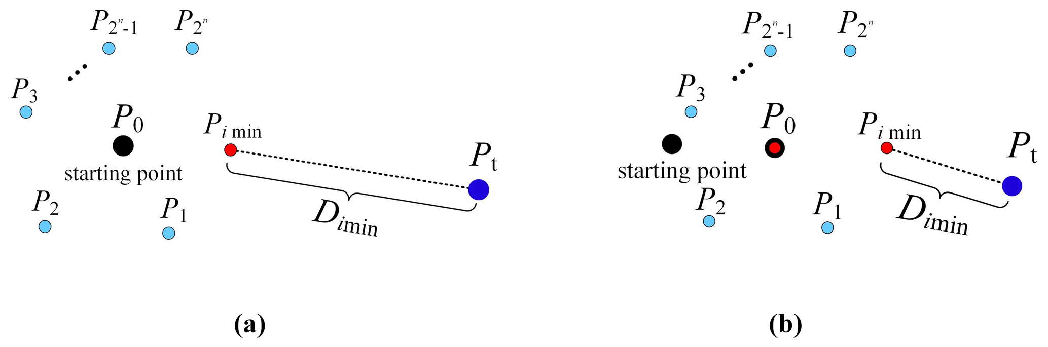
Figure 2Iterative calculation process of the joint perturbation method. (a) The first iteration. (b) The second iteration.
By this analogy, the joint perturbation coefficient matrix of a redundant manipulator with n DOFs is
In Eq. (9), , the elements of the first 2n−1 columns and the first row are all 1, and the elements of the last 2n−1 columns and the first row are all −1. When the joint motion priorities are determined, the joint perturbation coefficient matrix considering the joint motion priority can be obtained by multiplying row i of matrix Kn by ki. Similar to rotary joints, the motion priority of prismatic joints is set as kp, and the basic perturbation displacement as δd, and the coefficient of δd can be 1 or −1. When Δd=kpδd, the perturbation direction is positive, and when , the perturbation direction is negative. Therefore, this algorithm can be used for manipulators with prismatic joints.
2.4 Calculation of basic perturbation angle
The basic perturbation angle not only determines the amplitude of joint perturbation in an iterative calculation process but also plays a decisive role in the solving speed and accuracy of the algorithm. The smaller the basic perturbation angle, the higher the accuracy of the solution. As the number of iterations increases, the solving speed will decrease. Therefore, it is necessary to take a bigger basic perturbation angle while satisfying the solution accuracy. For a manipulator with n DOFs, the link lengths are , and then , and the maximum displacement Δs of the manipulator position for one perturbation should satisfy
where e is the maximum error allowed by the solution accuracy or predetermined. In this paper, the calculation formula of the basic perturbation angle is defined as
2.5 Inverse kinematics solution method
The joint angles after perturbation qti (i=1, 2, 3… 2n) can be calculated according to the joint perturbation coefficient matrix and the basic perturbation angle δθ.
In Eq. (12), the vector Kn(i) is the column i of the joint perturbation coefficient matrix Kn, so the pose of the manipulator Pi (i=1, 2, 3 …2n) can be calculated by
2n different poses ( can be obtained through one single operation for a redundant manipulator with n DOFs, and then the distance between each pose Pi and the target pose Pt can be calculated. The minimum of Di can be determined by comparisons, . Set the pose nearest to the target pose Pt as Pimin, so the joint variable corresponding to Pimin is qtimin. Further, set the pose Pimin as the starting pose and reassign P0 and q0 as , . The iterative calculations will continue for the target pose Pt until . When the iterative calculations end, the calculated joint variable qt is the inverse solution of the target pose Pt. The process of the iterative calculations from the starting pose P0 to the target pose Pt is shown in Fig. 2.
2.6 The main steps of the method
The main steps of the joint perturbation method are summarized as follows:
-
Establish the kinematics model of redundant manipulators with n DOFs.
-
Identify the current joint variables and calculate the corresponding manipulator pose P0.
-
Determine the target pose Pt and the priority of each joint motion ki according to actual task requirements.
-
Construct the joint perturbation coefficient matrix Kn, determine the basic perturbation angle δθ, and obtain the perturbation angle of each joint .
-
Calculate the joint angles after perturbation ().
-
Find all the poses Pi for the 2n kinds of possibilities by using the forward kinematics model of the manipulator.
-
Calculate the distance between the current manipulator pose Pi and the target pose Pt.
-
Obtain Dimin by comparison and verify whether is satisfied. If , the current joint angles are the joint variables qt corresponding to the target pose Pt. If , set the pose corresponding to joint variables qtimin as the starting pose and repeat steps 5–7.
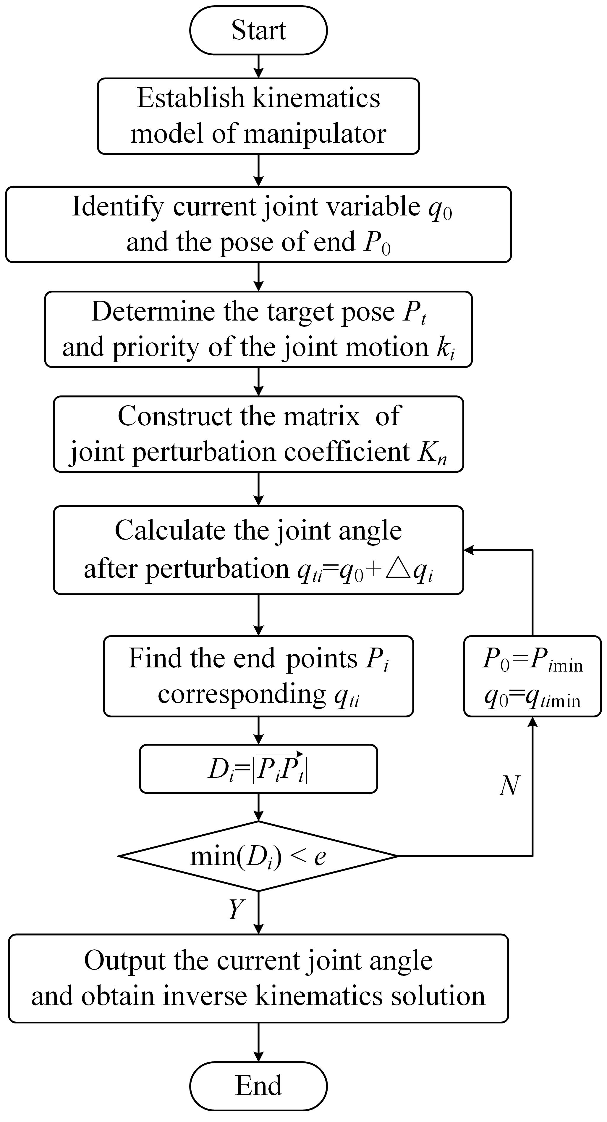
A flow chart of the method is shown in Fig. 3.
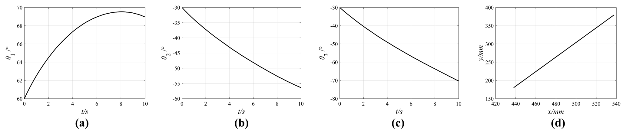
Figure 6Motion curves of the joints and the manipulator end. (a) The first joint. (b) The second joint. (c) The third joint. (d) Trajectory of the manipulator end.
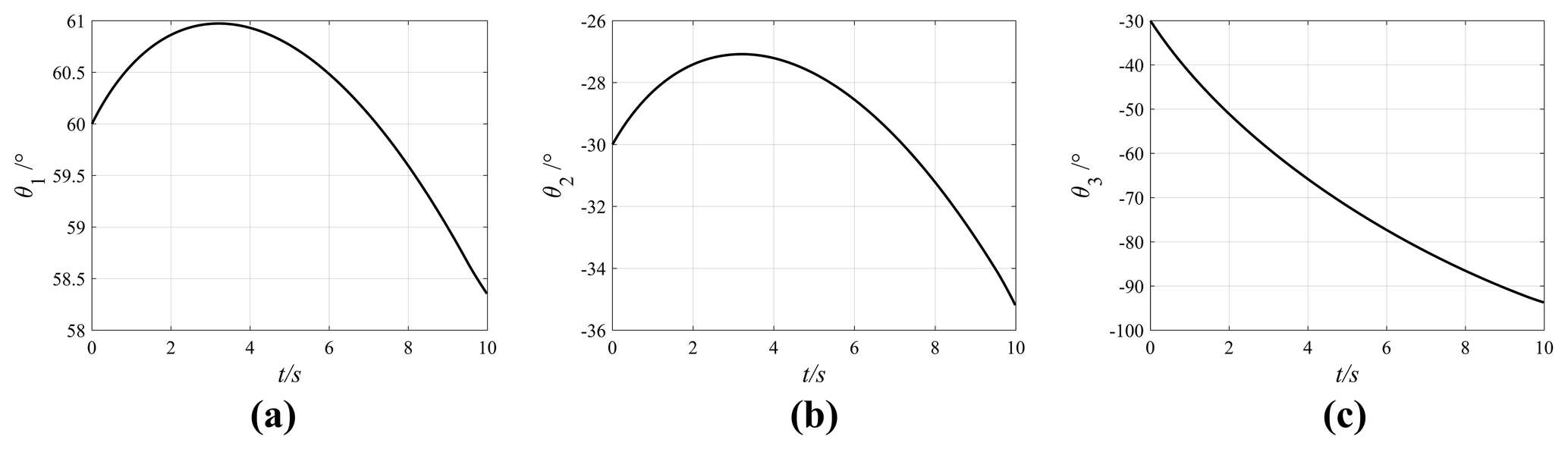
Figure 7Motion curves of the three joints (k1=0.2, k2=0.6, k3=1). (a) The first joint. (b) The second joint. (c) The third joint.
3.1 Simulation verification of a manipulator with 3 DOFs
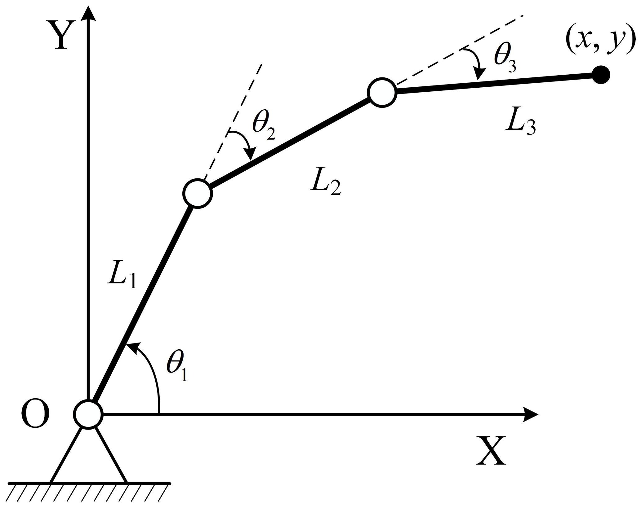
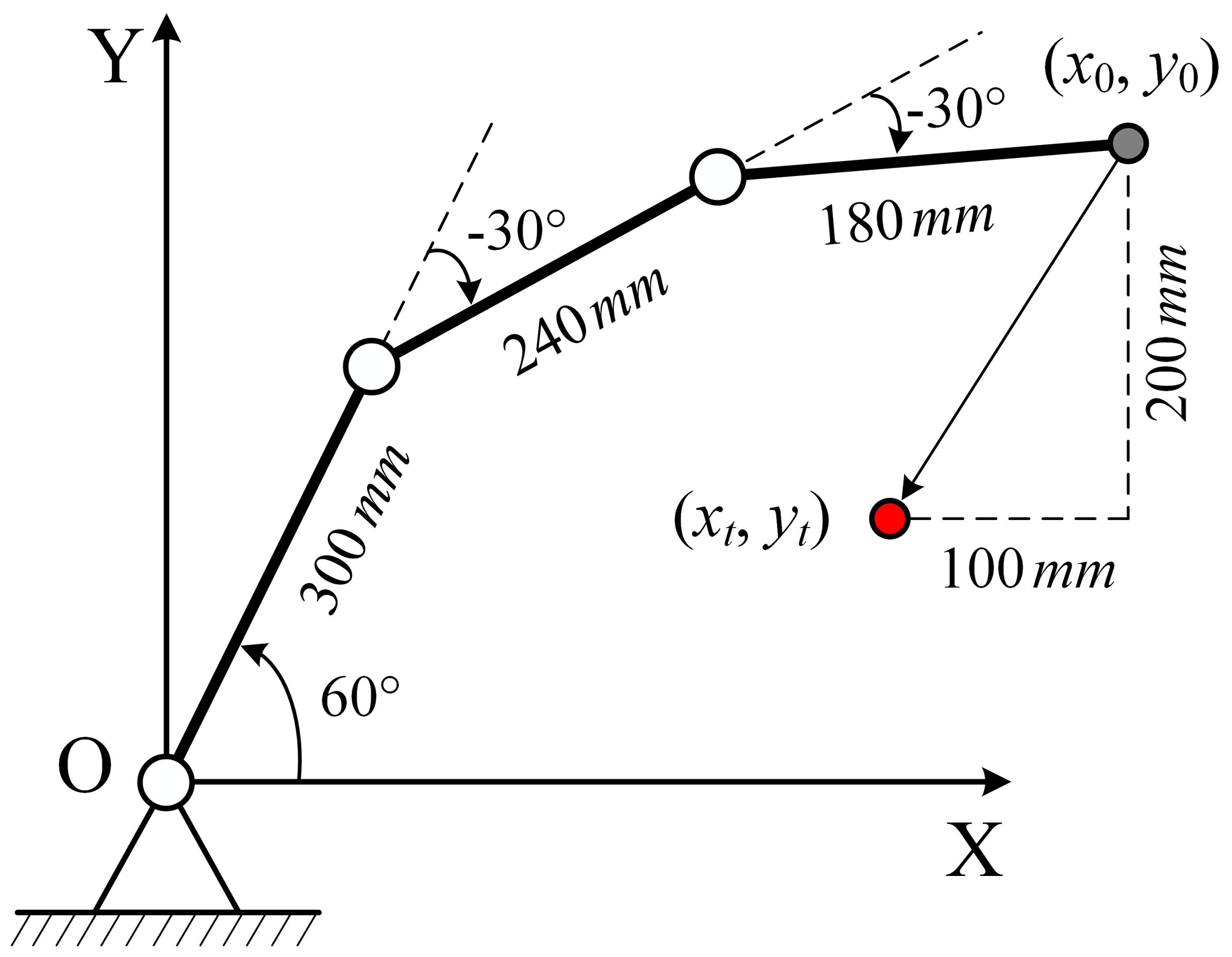
A planar manipulator with 3 DOFs is used to verify the inverse kinematics method based on joint perturbation. The schematic diagram of the manipulator mechanism is shown in Fig. 4. If only the position of the manipulator is considered, the mechanism is a planar manipulator with 1 redundant DOF.
The manipulator's position coordinates (x, y) can be obtained with the forward kinematics model.
The joint perturbation coefficient matrix of the manipulator is
The motion priorities of the three joints are k1, k2, and k3. The coefficient matrix considering the joint motion priorities is
Set the link lengths of the planar redundant manipulator as L1=300, L2=240, and L3=180 mm, and the current joint angles are θ01=60, , and . The current manipulator position coordinates P0(x0,y0) can be calculated with the current joint angles, with x0=537.8461 and y0=379.8076 mm. The target position coordinates are set to be Pt(437.8461,179.8076), as shown in Fig. 5.
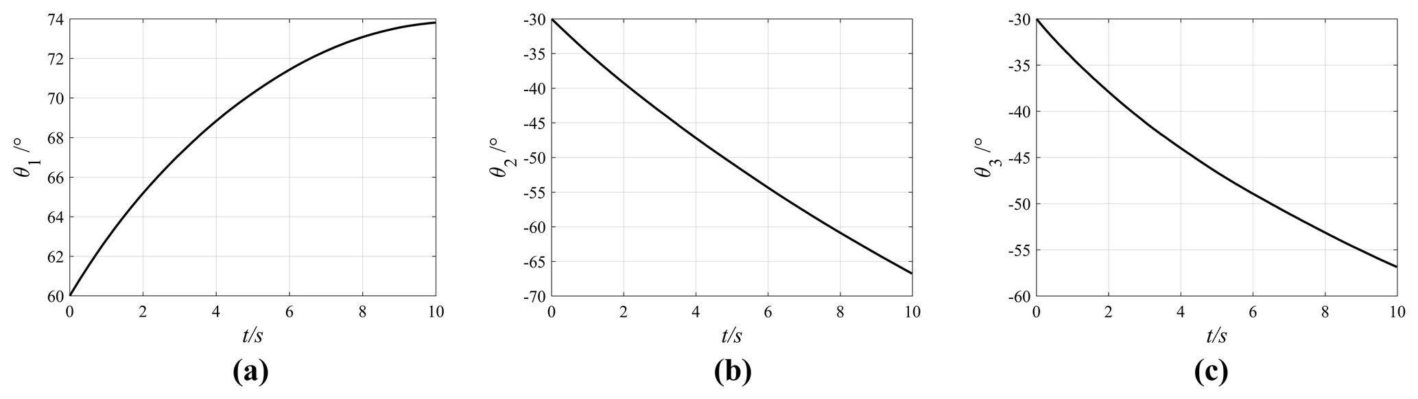
Figure 8Motion curves of the three joints (. (a) The first joint. (b) The second joint. (c) The third joint.

Figure 9Motion curves of the three joints (k1=0, ). (a) The first joint. (b) The second joint. (c) The third joint.
Let the motion priorities of the three joints be k1=0.6, k2=0.8, and k3=1.0, and set the allowable error e=0.01 mm and the basic perturbation angle as ∘. When the joint motion priorities are considered, the coefficient matrix K3 of the manipulator is
Therefore, the perturbation angle of each joint can be calculated as
Suppose that the manipulator takes t=10s to move from P0(x0,y0) to the target position Pt(xt,yt) along a straight line at a constant speed. The position changes of the manipulator and mm are given, and thus, the distance between the initial position and the target position is
Therefore, the velocity of the manipulator end is . The linear interpolation is performed in the motion path, and the interpolation period is taken as Δt=10 ms. So, the number of interpolations h is
Therefore, in an interpolation period, the displacement changes in x and y directions are as follows:
Calculate the path point Pb(xb,yb) of the manipulator from the initial position P0(x0,y0) to the target position Pt(xt,yt).
The first path point P1(x1,y1) is determined, where and . Next, and Pm(xm,ym) can be obtained through iterative calculations from the initial position P0(x0,y0) to the first path point P1(x1,y1). Further, qm and Pm(xm,ym) are assigned to q0 and P0(x0,y0), respectively, and then iterated to the second path point P2(x2,y2), where , . The iterative calculations and solutions will be repeated until .
In the process of iteration from the initial position P0(x0,y0) to the target position Pt(xt,yt), the joint angles corresponding to each path point can be calculated. The joint motion curves of the entire process are obtained after the iteration is completed, as shown in Fig. 6, where the abscissa represents the motion time and the ordinate represents the corresponding joint angles.
Table 1Comparisons of joint motions with different motion priorities.
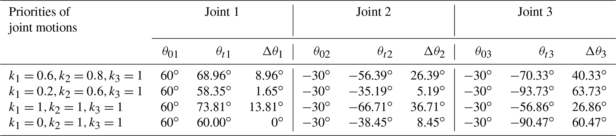
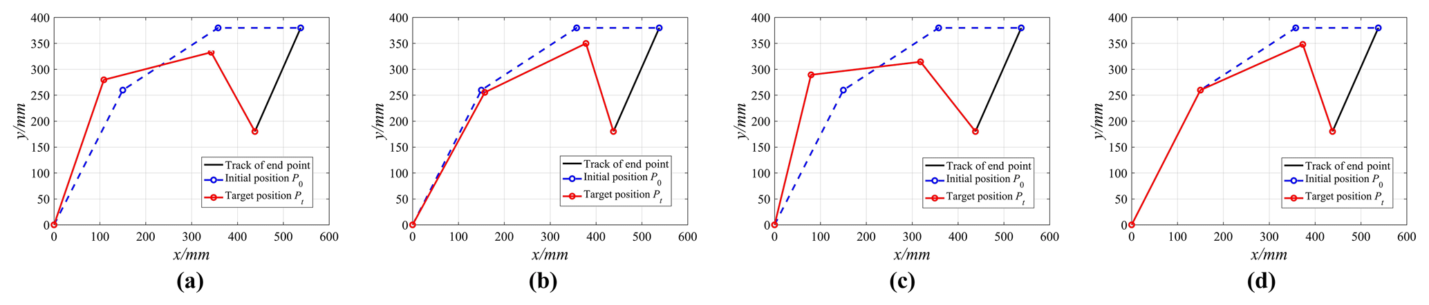
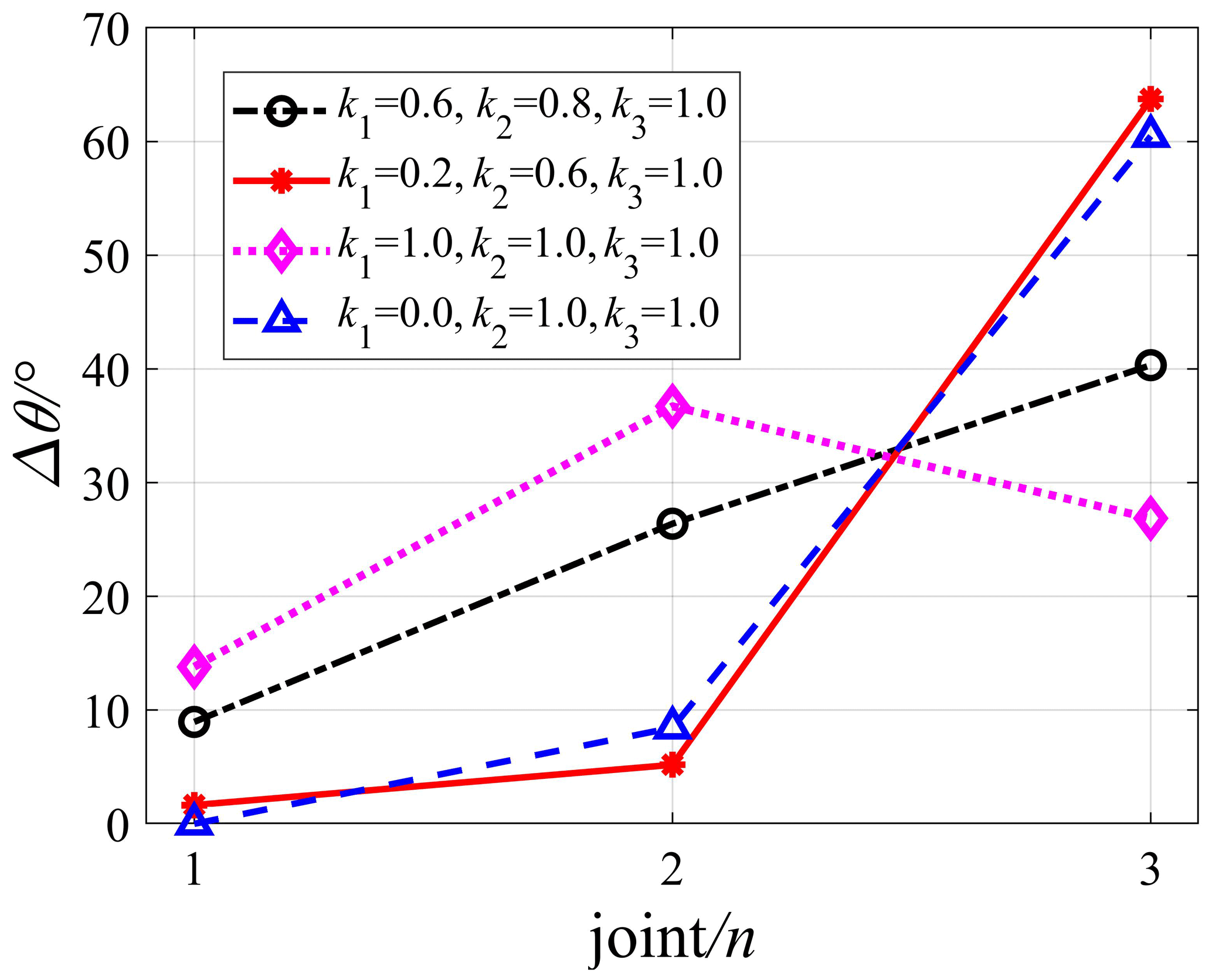
Figure 11Motion trajectories of the manipulator with different motion priorities. (a) k1=0.6, k2=0.8, k3=1.0. (b) k1=0.2, k2=0.6, k3=1.0. (c) . (d) k1=0, .
Figure 6 shows that the angle variations of the three joints are Δθ1=8.96, Δθ2=26.39, and , which comply with the setting of the motion priorities of the three joints, and the manipulator can move smoothly in the joint space.
Change the motion priority of each joint, by setting k1=0.2, k2=0.6, k3=1, , and k1=0, while keeping other parameters unchanged. The effect of the joint motion priorities on joint motions is obtained through simulations. The joint motion curves under different motion priorities are shown in Figs. 7, 8, and 9.
After analysing the joint motion curves in the four cases, the angle variation of each joint under different motion priorities can be obtained, as shown in Fig. 10, where the abscissa represents the three joint motions of the manipulator and the ordinate represents the magnitude of the angle variation of each joint. The specific values are shown in Table 1. In this Table, θ01, θ02, and θ03 represent the initial joint angles; θt1, θt2, and θt3 represent the joint angles corresponding to the target position; and Δθ1, Δθ2, and Δθ3 represent the angle variations of three joints, ().

The effect of the joint motion priority on joint motions can be obtained according to Table 1 and Fig. 11. Figure 11a and b show that the motion priority of the first joint decreases by Δk1=0.4, and the variation of joint motion changes from 8.96 to 1.65∘ with a decrease of 81.58 %; the motion priority of the second joint decreases by Δk2=0.2, and the corresponding variation of joint motion changes from 26.39 to 5.19∘ with a decrease of 80.33 %, while the variation of the third joint motion changes from 40.33 to 63.73∘ with an increase of 58.02 %. Figure 11a and c show that the motion priority of the first joint increases by Δk1=0.4, and the variation of joint motion changes from 8.96 to 13.81∘ with an increase of 54.13 %; the motion priority of the second joint increases by Δk2=0.2, and the corresponding variation of joint motion changes from 26.39 to 36.71∘ with an increase of 39.11 %, while the variation of the third joint motion changes from 40.33 to 26.86∘ with a decrease of 33.34 %. Figure 11d shows that when the motion priority of the first joint is 0 (k1=0), the first joint will remain stationary, and the corresponding motion is completed by the second joint and the third joint.
3.2 Simulation verification of a manipulator with 7 DOFs
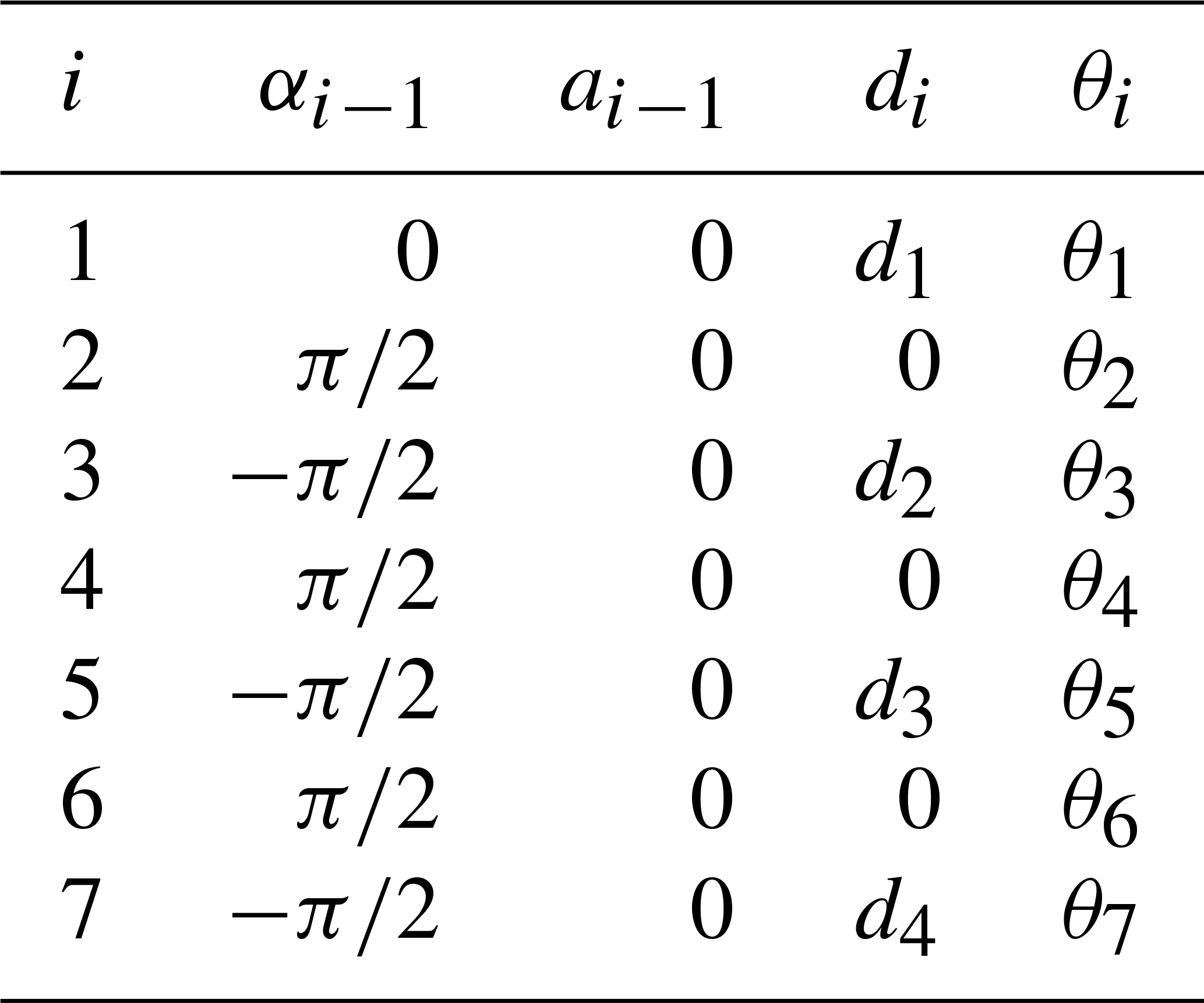
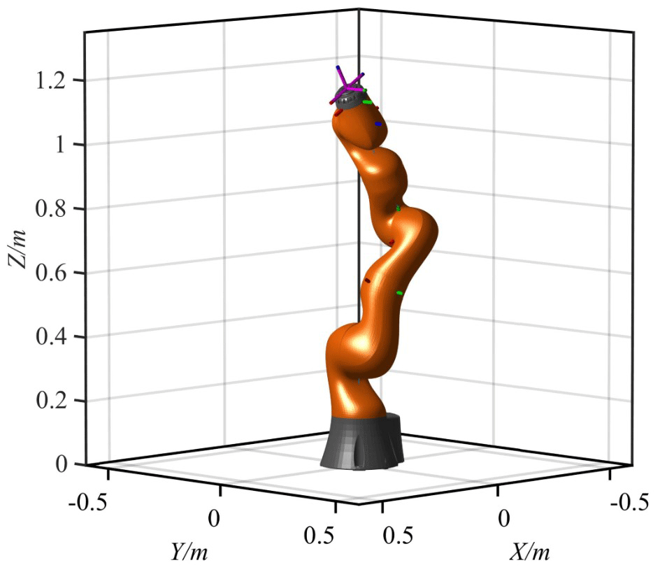
To verify the universality of the algorithm, a redundant manipulator with 7 DOFs (KUKA iiwa) is used for simulation verification. First, the model of the redundant manipulator is obtained using the D–H method, as shown in Fig. 12, where d1=340, d2=400, d3=400, and d4=126.6 mm. The D–H parameters are shown in Table 2.
Set the initial joint values as , and the coordinates of the manipulator end can be obtained by the forward kinematics, P0=[63.301142.5] mm, as shown in Fig. 13.
The manipulator will take t=10 s to move from the initial position to the target position . Set the allowable error as e=0.01 mm, and calculate the basic perturbation angle ∘.
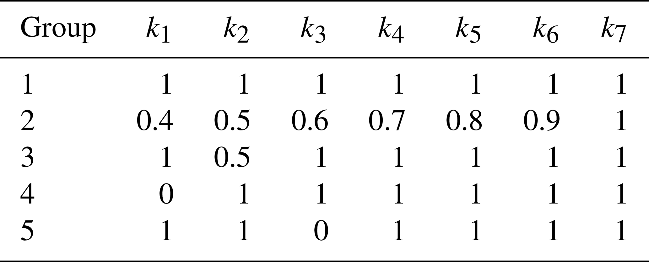
The interpolation period is set as Δt=10 ms, and thus the number of interpolations is h=1000. Therefore, the displacement changes in x, y, and z directions are dx=0.2, , and mm, respectively. The simulations are divided into five groups for comparisons, and the joint motion priorities of each group are set as shown in Table 3.
Using the motion priorities of the five groups while keeping other parameters unchanged, the joint motion curves under different motion priorities are shown in Figs. 14, 15, 16, 17, and 18.
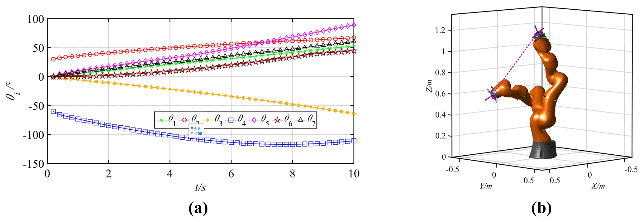
Figure 14Motion curves of the joints and the manipulator (. (a) Joint motion curves. (b) Trajectory of the manipulator.
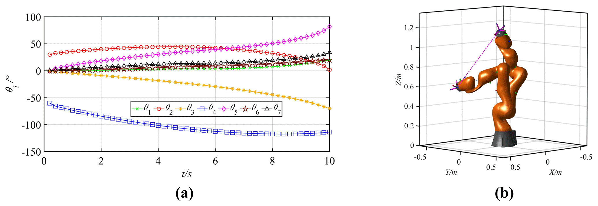
Figure 15Motion curves of the joints and the manipulator (k1=0.4, k2=0.5, k3=0.6, k4=0.7, k5=0.8, k6=0.9, k7=1.0). (a) Joint motion curves. (b) Trajectory of the manipulator.
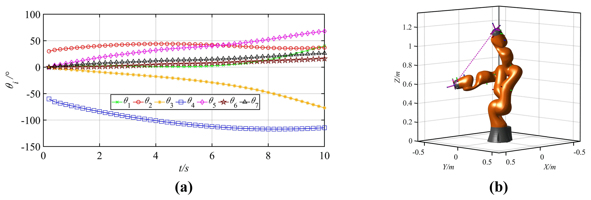
Figure 16Motion curves of the joints and the manipulator (k2=0.5, ). (a) Joint motion curves. (b) Trajectory of the manipulator.
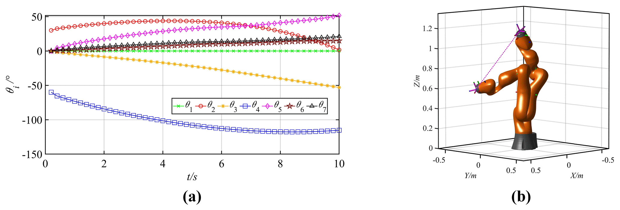
Figure 17Motion curves of the joints and the manipulator (k1=0, ). (a) Joint motion curves. (b) Trajectory of the manipulator.
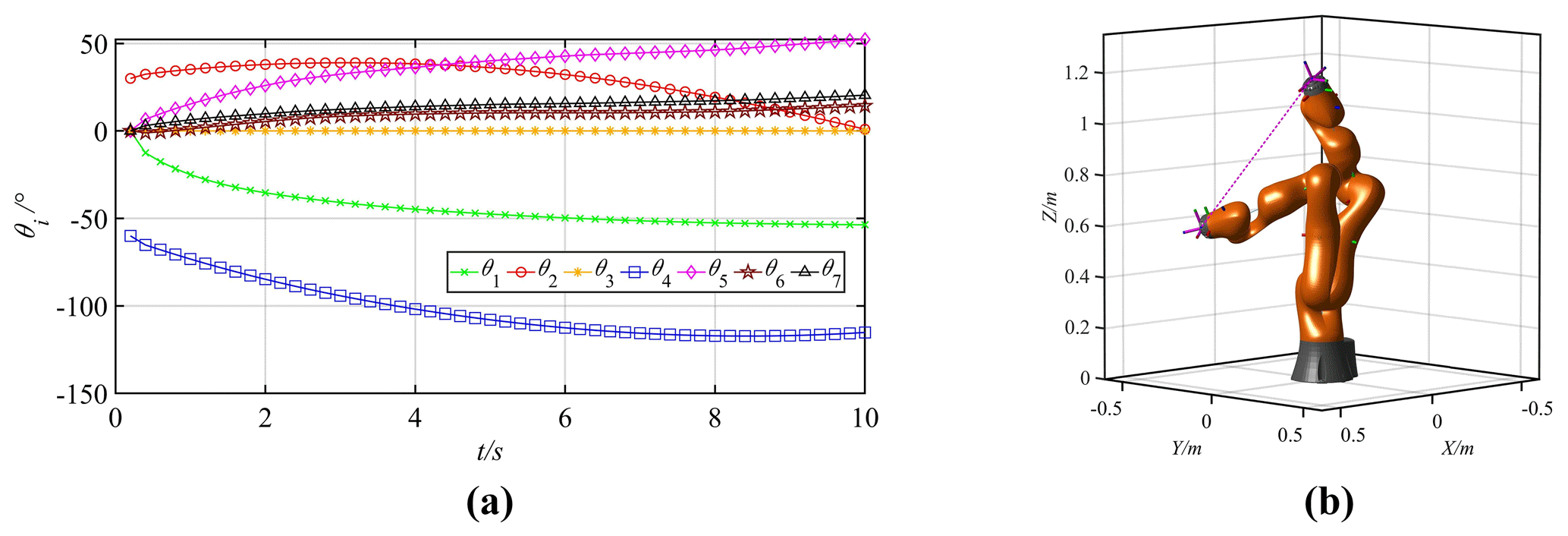
Figure 18Motion curves of the joints and the manipulator (k3=0, ). (a) Joint motion curves. (b) Trajectory of the manipulator.
The angle variation of each joint under different motion priorities can be obtained, as shown in Table 4. In this table, θ0i represents the initial joint angles, θti represents the joint angles corresponding to the target position, and Δθi represents the angle variations of seven joints, .
Table 4Comparisons of joint motions with different motion priorities.
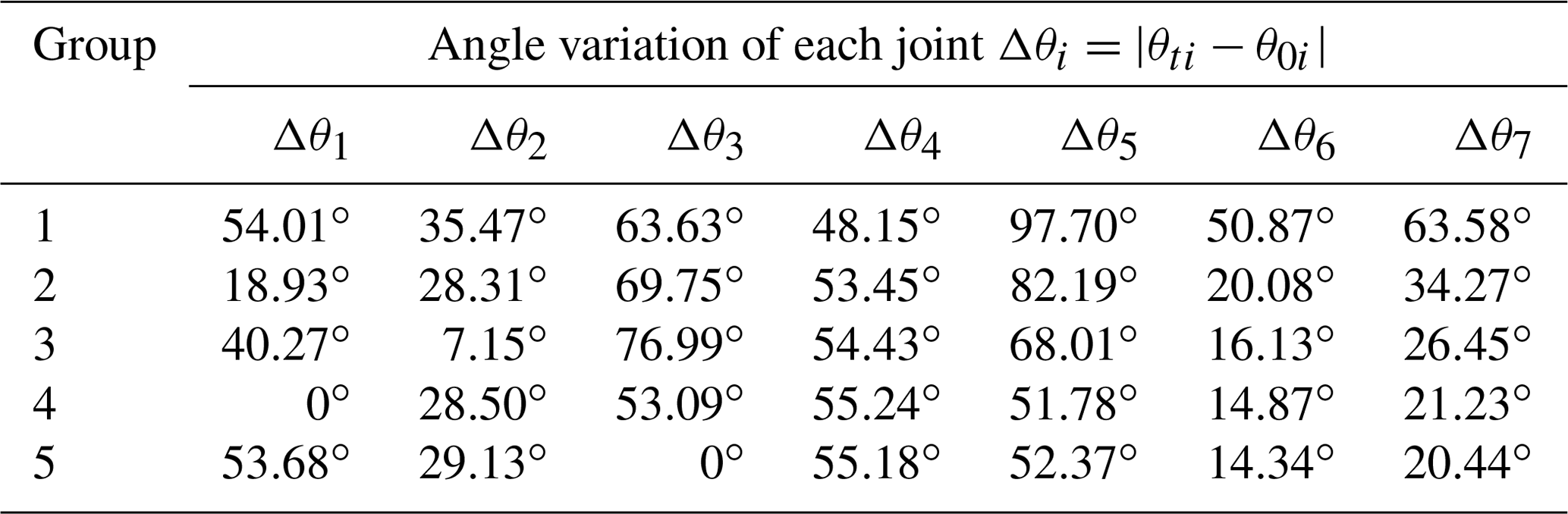

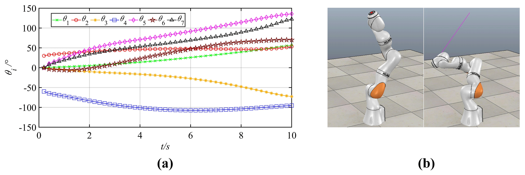
Figure 19Joint motion curves and simulation process. (a) Joint motion curves. (b) Initial and target poses.
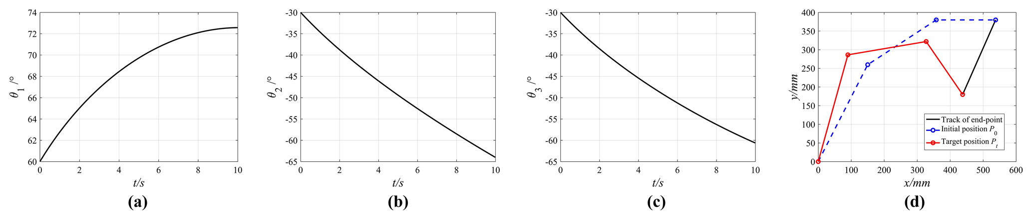
Figure 20Motion curves of the joints and the manipulator (3 DOFs). (a) The first joint. (b) The second joint. (c) The third joint. (d) Trajectory of the manipulator.
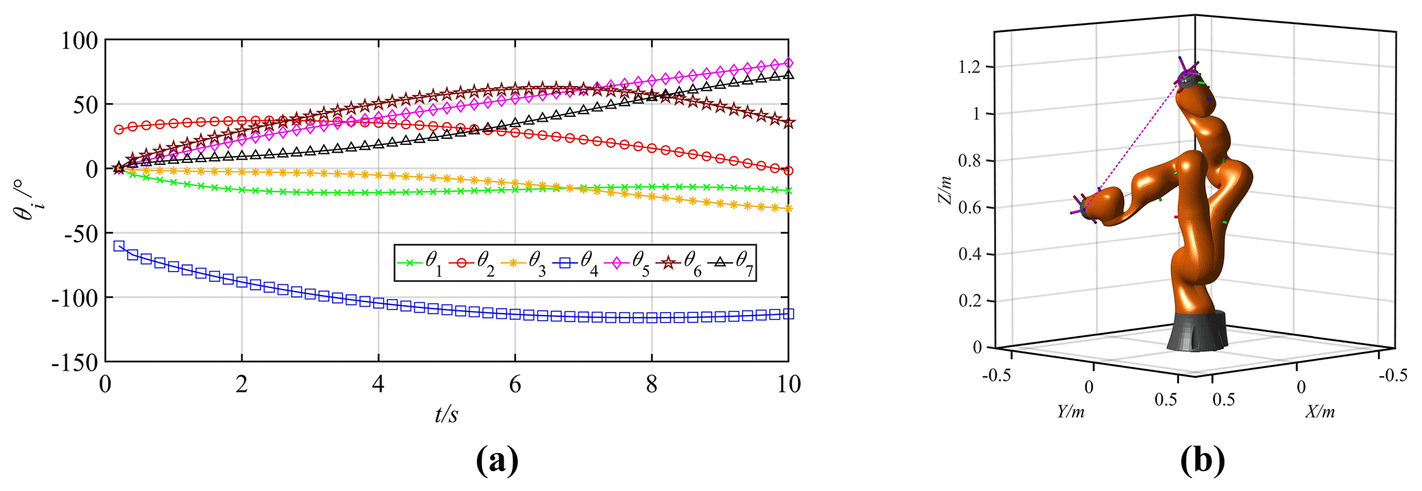
Figure 21Motion curves of the joints and the manipulator (7 DOFs). (a) Joint motion curves. (b) Trajectory of the manipulator.
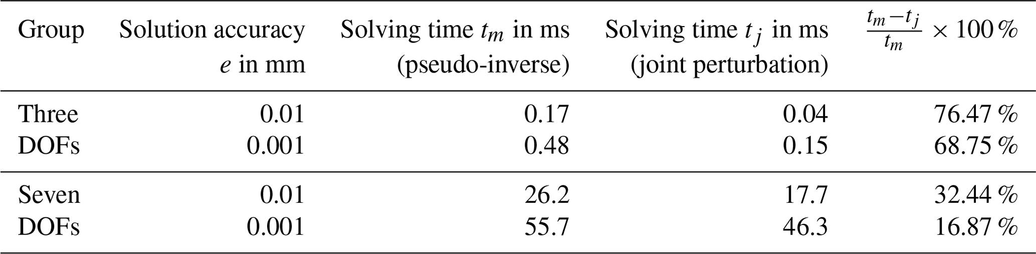
Table 6Solving time for the Jacobian pseudo-inverse method and the perturbation method.
Because the joint motion priorities are the same in Group 1, the motion angle of each joint is relatively averaged. In Group 2, the motion priorities of big joints are relatively low, while the motion priorities of small joints are relatively high. Then, the motion amplitudes of the first and the second joints decrease significantly. Comparing Groups 1 and 3 shows that the motion priority of the second joint is reduced to 0.5, and the corresponding angle variation is decreased from 35.47 to 7.15∘. In Groups 4 and 5, the motion priorities of the first joint and the third joint are set as 0, so the corresponding joints remain stationary.
Solving inverse kinematics of redundant manipulators with 3 DOFs and 7 DOFs shows consistent simulation results. The higher the relative joint motion priority, the bigger the joint motion angle, and in contrast, the lower the relative joint motion priority, the smaller the joint motion angle. When the joints have the same priority, the motion angle of each joint will be relatively averaged. In particular, when the motion priority of a joint is zero, the joint motion angle is zero, too. Therefore, the motion range of a joint can be controlled by changing the motion priority. Hence, the joint perturbation method can be used to deal with joint limit avoidance when calculating the inverse kinematics solution of a redundant manipulator. For a manipulator with n DOFs, assume that the motion range limit of joint i is , then the joint angles qi satisfy the following conditions:
Normally, the constraint interval of a joint angle is symmetrical; that is . Then, the motion priority of joint i can be defined as
Therefore, ki approaches 0 when qi approaches the joint limit; ki=1 when .
3.3 Simulation experiment based on CoppeliaSim
Take the manipulator with 7 DOFs, KUKA iiwa, to perform the same motion task of Sect. 3.2 in CoppeliaSim, of which simulation results are widely acknowledged to have a high consistency with actual experiments. The joint motion ranges of the manipulator are shown in Table 5, and the real-time joint motion priorities are calculated according to formula (25). The joint curves are obtained as shown in Fig. 19a. All joints do not exceed their motion ranges.
The joint curves were imported into CoppeliaSim as the driving function to complete the experimental tasks, as shown in Fig. 19b. During the movement, the manipulator ran smoothly and completed the task of a linear trajectory.
3.4 Real-time characteristic analyses
The Jacobian pseudo-inverse method is widely used to solve the inverse kinematics of redundant manipulators. The real-time characteristic comparisons will be conducted between it and the proposed method. The inverse kinematics solution of the redundant manipulator with n DOFs is
where is the joint velocity, is the velocity of the manipulator, J+ is the generalized inverse matrix of J, α is the scalar coefficient, is an arbitrary vector, and is the null space vector which represents the self-motion of the manipulator in the null space and satisfies .
All the conditions and motion tasks of the two manipulators (3 DOFs and 7 DOFs) are the same as those of the two in Sect. 3.1 and 3.2 respectively. In this paper, the minimum norm solution of joint velocity, , is adopted, and the joint motion curves are obtained as shown in Figs. 20 and 21.
For the planar manipulator with 3 DOFs and the space manipulator with 7 DOFs, different solution accuracy values (e=0.01 and e=0.001 mm, respectively) are set. The solving times of the two methods are calculated with MATLAB, and the results are shown in Table 6. According to Table 6, both methods can reach the microsecond level, and the solving time of the perturbation method tj is shorter than that of the Jacobian pseudo-inverse method tm. So, the joint perturbation method has better efficiency and real-time performance than the Jacobian pseudo-inverse method. However, with the improvement of the solution accuracy and the increase of the degrees of freedom, the calculation times of the both methods increase significantly, and the preponderance of the joint perturbation method over the Jacobian pseudo-inverse method has a downward trend.
The inverse kinematics solution of redundant manipulators usually takes a considerable amount of time to calculate. Aiming at improving the solving efficiency of inverse kinematics, this paper first defines the concepts of joint motion priority and joint perturbation coefficient matrix, then proposes an algorithm based on joint perturbation to solve the inverse solution of redundant manipulators. The feasibility and real-time characteristics of the algorithm were verified through simulations of two types of redundant manipulators with 3 DOFs and 7 DOFs, respectively. The following conclusions are obtained:
-
The magnitude of motion priority determines the level of joint motion priority. When a redundant manipulator performs a specific task, a higher joint motion priority leads to a bigger joint motion angle, while a lower joint motion priority results in a smaller joint motion angle. In particular, when the joint motion priority is zero, the joint motion angle is also zero. Therefore, the motion of a joint can be controlled by setting different joint motion priorities, which can be used in obstacle avoidance and joint limit avoidance.
-
The proposed algorithm has universality and has no restrictions on the structure and DOFs of manipulators. Moreover, the solving process of this algorithm only involves the forward kinematics, which can avoid the pseudo-inverse calculations of the Jacobian matrix and significantly reduce the solving complexity, so it has a better real-time performance than the Jacobian pseudo-inverse method. The method can be used in real applications to speed up the work cycle and improve production efficiency.
-
However, the proposed algorithm also has certain limitations, and the calculation load will increase exponentially with the increase of the degrees of freedom of a manipulator. In the future, we will continue to study the algorithm in the optimization of joint motion priorities and experimental verifications.
All the data used in this paper can be obtained upon request from the corresponding author.
QX contributed to the conception of the study, performed the validation, and wrote the original draft. QZ contributed to the funding acquisition and project administration. QX and QZ jointly completed data curation, review, and editing.
The authors declare that they have no conflict of interest.
Thanks are due to Xinyang Tian for assistance with the simulation and to Xiangzhen Chen for valuable discussion. Thanks are expressed to the research platform provided by the Laboratory of Complex Mechanism and Intelligent Control.
This research has been supported by the Beijing Natural Science Foundation, Haidian Original Innovation Joint Fund Project (grant no. L172015).
This paper was edited by Daniel Condurache and reviewed by Giuseppe Carbone, Miguel Díaz-Rodríguez, and one anonymous referee.
Akbaripour, H. and Masehian, E.: Semi-lazy probabilistic roadmap: a parameter-tuned, resilient and robust path planning method for manipulator robots, Int. J. Adv. Manuf. Technol, 89, 1401–1430, https://doi.org/10.1007/s00170-016-9074-6, 2017.
Aouache, M., Maoudj, A., and Akli, I.: Human-robot interaction in industrial collaborative robotics: a literature review of the decade 2008–2017, Adv. Robotics, 33, 764–799, https://doi.org/10.1080/01691864.2019.1636714, 2019.
Ayusawa, K. and Nakamura, Y.: Fast inverse kinematics algorithm for large DOF system with decomposed gradient computation based on recursive formulation of equilibrium, in: Proc. IROS, Vilamoura, Portugal, 3447–3452, https://doi.org/10.1109/IROS.2012.6385780, 2012.
Damas, B. J. and Santos, V.: An online algorithm for simultaneously learning forward and inverse kinematics, in: Proc. IROS, Vilamoura, Portugal, 1499–1506, https://doi.org/10.1109/IROS.2012.6386156, 2012.
Dasgupta, B., Gupta, A., and Singla, E.: A variational approach to path planning for hyper-redundant manipulators, Robot. Auto. Syst., 2, 194–201, https://doi.org/10.1016/j.robot.2008.05.001, 2009.
Faria, C., Ferreira, F., Erhagen, W., Sérgio, M., and Estela, B.: Position-based kinematics for 7-dof serial manipulators with global configuration control, joint limit and singularity avoidance, Mech. Mach. Theory., 121, 317–334, https://doi.org/10.1016/j.mechmachtheory.2017.10.025, 2018.
Hayashibe, M., Suzuki, N., and Hashizume, M.: Robotic surgery setup simulation with the integration of inverse-kinematics computation and medical imaging, Comput. Meth. Prog. Bio., 1, 63–72, https://doi.org/10.1016/j.cmpb.2006.04.010, 2006.
Jia, Q. X., Zhang, L., Chen, G., and Sun, H. X.: Pre-impact trajectory optimization of redundant space manipulator with multi-target fusion, J. Astronautics, 6, 639–647, https://doi.org/10.3873/j.issn.1000-1328.2014.06.004, 2014.
Kalra, P., Mahapatra, P. B., and Aggareal, D. K.: An evolutionary approach for solving the multimodal inverse kinematics problem of industrial robots, Mech. Mach. Theory, 41, 1213–1229, https://doi.org/10.1016/j.mechmachtheory.2005.11.005, 2006.
Korein, J. U. and Badler, N. I.: Techniques for generating the goal-directed motion of articulated structures, IEEE Comput. Graph., 9, 71–81, https://doi.org/10.1109/MCG.1982.1674498, 1982.
Jiokou Kouabon,A. G., Melingui, A., Mvogo Ahanda, J. J. B., Lakhal, O., Coelen, V., Kom, M., and Merzouki, R.: A Learning Framework to inverse kinematics of high DOF redundant manipulators, Mech. Mach. Theory, 153, 103978, https://doi.org/10.1016/j.mechmachtheory.2020.103978, 2020.
Kuhlemann, I., Schweikard, A., Jauer, P., and Ernst, F.: Robust inverse kinematics by configuration control for redundant manipulators with seven DOF, in: Proc. International Conference on Control, Automation and Robotics, Hong Kong, 49–55, https://doi.org/10.1109/ICCAR.2016.7486697, 2016.
Kumar, S., Sukavanam, N., and Balasubramanian, R.: An optimization approach to solve the inverse kinematics of redundant manipulator, Int. J. Inf. Syst. Sci., 4, 414–423, https://doi.org/10.13140/2.1.2666.9125, 2010.
Liu, W., Chen, D., and Steil, J.: Analytical inverse kinematics solver for anthropomorphic 7-dof redundant manipulators with human-like configuration constraints, J. Intell. Robot. Syst., 86, 63–79, https://doi.org/10.1007/s10846-016-0449-6, 2017.
Lopezfranco, C., Hernandezbarragan, J., and Alanis, A. Y.: Inverse kinematics of mobile manipulators based on differential evolution, Int. J. Adv. Robot. Syst., 1, 1–22, https://doi.org/10.1177/1729881417752738, 2018.
Lv, Y. and Liu, F.: Application Analysis of Generalized and Modified D-H Method in Kinematic Modeling, Comput. Syst. Appl., 5, 197–202, 2016.
Maciejewski, A. A. and Klein, C. A.: Obstacle avoidance for kinematically redundant manipulators in dynamically varying environments, Int. J. Robot. Res., 3, 109–117, https://doi.org/10.1177/027836498500400308, 1985.
Mohamed, H. A., Yahya, S., Moghavvemi, M., and Yang, S. S.: A new inverse kinematics method for three dimensional redundant manipulators, in: Proc. IEEE ICCAS-SICE, Fukuoka, Japan, 1557–1562, 2009.
Omrcen, D. and Zlajpah, L.: Compensation of velocity and/or acceleration joint saturation applied to redundant manipulator, Robot. Auto. Syst., 55, 337–344, https://doi.org/10.1016/j.robot.2006.10.001, 2007.
Park, H., Kwak, B., and Bae, J.: Inverse Kinematics Analysis and COG Trajectory Planning Algorithms for Stable Walking of a Quadruped Robot with Redundant DOFs, J. Bionic Eng., 15, 610–622, https://doi.org/10.1007/s42235-018-0050-8, 2018.
Tian, X. Y., Xu, Q. H., and Zhan, Q.: An analytical inverse kinematics solution with joint limits avoidance of 7-DOF anthropomorphic manipulators without offset, J. Frankl. Inst., 358, 1252–1272, https://doi.org/10.1016/j.jfranklin.2020.11.020, 2020.
Tolani, D., Goswami, A., and Badler, N. I.: Real-time inverse kinematics techniques for anthropomorphic limbs, Graph. Models, 5, 353–388, https://doi.org/10.1006/gmod.2000.0528, 2000.
Umar, A., Shi, Z., and Wang, W.: A novel mutating pso based solution for inverse kinematic analysis of multi degree-of-freedom robot manipulators, in: Proc. ICAICA, Dalian, China, 459–463, https://doi.org/10.1109/ICAICA.2019.8873449, 2019.
Xia, Y. and Wang, J.: A dual neural network for kinematic control of redundant robot manipulators, IEEE Trans. Syst. Man Cybern., 1, 147–154, https://doi.org/10.1109/3477.907574, 2001.
Xu, H., Xie, X., and Zhuang, J.: Global Time-energy optimal planning of industrial robot trajectories, J. Mech. Eng., 9, 19–25, https://doi.org/10.3901/JME.2010.09.019, 2010.
Zaplana, I. and Basanez, L.: A novel closed-formed solution for the inverse kinematics of redundant manipulators through workspace analysis, Mech. Mach. Theory, 121, 829–843, https://doi.org/10.1016/j.mechmachtheory.2017.12.005, 2018.
Zeng, Z., Chen, Z., Shu, G., and Chen, Q.: Optimization of analytical inverse kinematic solution for redundant manipulators using GA-PSO algorithm, IEEE Industrial Cyber-Physical Systems, 5, 446–451, https://doi.org/10.1109/ICPHYS.2018.8390746, 2018.
Zu, D., Wu, Z., and Tan, D.: Efficient inverse kinematic solution for redundant manipulator, China, J. Mech. Eng.-En., 6, 71–75, https://doi.org/10.3901/JME.2005.06.071, 2005.