Heat transfer and MHD flow of non-newtonian Maxwell fluid through a parallel plate channel: analytical and numerical solution

Analytical and numerical analyses have been performed to study the problem of magneto-hydrodynamic (MHD) flow and heat transfer of an upper-convected Maxwell fluid in a parallel plate channel. The governing equations of continuity, momentum and energy are reduced to two ordinary differential equation forms by introducing a similarity transformation. The Homotopy Analysis Method (HAM), Homotopy Perturbation Method (HPM) and fourth-order Runge-Kutta numerical method (NUM) are used to solve this problem. Also, velocity and temperature fields have been computed and shown graphically for various values of the physical parameters. The objectives of the present work are to investigate the effect of the Deborah numbers (De), Hartman electric number (Ha), Reynolds number (Re_w) and Prandtl number (Pr) on the velocity and temperature fields. As an important outcome, it is observed that increasing the Hartman number leads to a reduction in the velocity values while increasing the Deborah number has negligible impact on the velocity increment.

1 Introduction

Non-Newtonian fluid flow is a fast-growing field of interest due to its various applications in different fields of engineering (Rivlin and Ericksen, 1955). The problem with this type of fluid is that there is not a single constitutive equation due to various rheological parameters appearing in such fluids. Therefore, different models have been developed in the forms of (i) differential type, (ii) rate type and (iii) integral type (Hayat and Awais, 2011; Hayat et al., 2012). The dynamics of materials with the properties of elasticity and viscosity is a fundamental topic in fluid dynamics. This kind of materials is referred to as Maxwell fluid (Mukhopadhyay, 2012; Adegbie et al., 2015). This model categorized as a subclass of rate type fluids can predict the stress relaxation. The Upper Convected Maxwell (UCM) model is the generalization of the Maxwell material for the case of large deformation using the upper convected time derivative.

Several researchers have investigated the application of MHD flow in different industrial applications (Recebli et al., 2013, 2015; Selimli et al., 2015; Hayat et al., 2017). Reviewing the literature indicates the importance of MHD flow through parallel channels. Hayat et al. (2006) was among the first who studied the MHD flow of an upper convected Maxwell (UCM) fluid over a porous stretching sheet using homotopy analysis method (HAM). Raftari and Yildirim (2010) proposed a novel analytical model (homotopy perturbation method (HPM) to analyze the same problem investigated by (Hayat et al., 2006). Switching from the non-rotating flow to rotating one was made by Sajid et al. (2011). They advanced the knowledge in this field by considering the effect of rotation parameter on the overall performance of the UCM. They concluded that the rotation parameter can help in controlling the thickness of boundary layer. Compared to the analytical techniques used by (Hayat et al., 2006; Raftari and Yildirim, 2010), Abel et al. (2012) proposed a numerical scheme, fourth order Runge–Kutta method, to examine the MHD flow for UCM Maxwell over a stretching sheet. These studies were focused on the no-slip boundary condition imposed along the flat plate. Therefore, Abbasi and Rahimipetroudi (2013) aimed at improving the models in this field by considering the slip boundary condition of an UCM Maxwell fluid via HPM. More complexity was added to the available models by Nadeem et al. (2014). They looked at the performance of the MHD boundary layer flow of a Maxwell fluid with nanoparticles. Afify and Elgazery (2016) extended the problem by Nadeem et al. (2014) by adding the chemical reaction into their model. In a more recent research, effects of thermal radiation (Hayat et al., 2011b) and mass transfer (Hayat et al., 2011a) were studied on the MHD flow of the UCM fluid with porosity in the channel walls.

In recent decades, many attempts have been made to develop analytical methods for solving such nonlinear equations. Analytical techniques such as HPM (Abbasi and Rahimipetroudi, 2013; He, 2000; Abbasi et al., 2014) and HAM (Hayat et al., 2006; Abbasi et al., 2014, 2016; Turkyilmazoglu, 2011) have been successfully applied to solve many types of nonlinear problems. The aim of this study is to investigate the effect of physical parameters on a steady flow of an upper-convected Maxwell fluid in a channel in the presence of an external magnetic field. In addition, the convergence of the series solution is also explicitly discussed. The obtained results from the analytical solution have been compared with the numerical data and the comparison reveals the capability, effectiveness and convenience of the Homotopy Analysis Method (HAM) and the Homotopy Perturbation Method (HPM) methods in solving the stated problem. Finally, the effect of dominating parameters on the MHD flow and heat transfer of UCM in a parallel plate is discussed.

2 Problem statement and mathematical formulation

Figure 1 illustrates the schematic diagram of the magneto-hydrodynamic (MHD) flow of an incompressible UCM fluid in a parallel plate channel. As seen, the x^∗-axis is taken along the centerline of the channel, parallel to the channel surfaces, and the y^∗-axis is transverse to this. The inter-plate region contains an incompressible two-dimensional steady, laminar UCM viscoelastic fluid flow. The flow is symmetric in X-axis direction. The steady state flow occurs in the channel with the fluid suction and injection taking place at both plates with velocityV_w. The fluid injection and suction take place through the walls where V_w>0 stands for suction and V_w<0 stands for injection. The walls of the channel are at $y^{\ast }=H$ and $y^{\ast }=-H$ (where 2H is the channel height). Here u^∗ and v^∗ are the velocities components in the x^∗ and y^∗ directions, respectively.

Figure 1 Schematic diagram and the coordinate system for the considered flow.

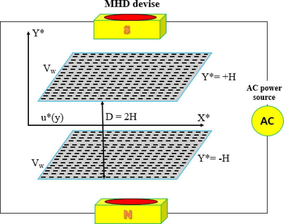
A uniform magnetic field, B₀, is imposed along the y^∗-axis. The constitutive equation for a Maxwell fluid is (Bég and Makinde, 2010):

$$\begin{array}{}\text{(1)}& \mathit{\tau }+{\mathit{\lambda }}_{\mathrm{1}}\widehat{\mathit{\tau }}={\mathit{\mu }}_{\mathrm{0}}\mathit{\gamma }\end{array}$$

where τ, λ₁, μ₀ and γ are the extra stress tensor, relaxation time, low-shear viscosity and the rate-of-strain tensor, respectively. The upper convected time derivative of the stress tensor $\widehat{\mathit{\tau }}$is formulated by:

$$\begin{array}{}\text{(2)}& \widehat{\mathit{\tau }}={\displaystyle \frac{\partial \mathit{\tau }}{\partial t}}+v\cdot \mathrm{\nabla }\mathit{\tau }-{\left(\mathrm{\nabla }v\right)}^T\cdot \mathit{\tau }-\mathit{\tau }\cdot \mathrm{\nabla }v\end{array}$$

where t, v, (⋅)^T and ∇v denote time, velocity vector, transpose of tensor and fluid velocity gradient tensor, respectively. Governing equations take the following form for the UCM fluid by implementing the shear stress strain tensor from Eqs. (1) and (2) (Wehgal and Ashraf, 2012; Hayat and Wang, 2003):

$$\begin{array}{ll}\text{(3)}& {\displaystyle }& {\displaystyle \frac{\partial u^{\ast }}{\partial x^{\ast }}}+{\displaystyle \frac{\partial {\mathit{\nu }}^{\ast }}{\partial y^{\ast }}}=\mathrm{0}{\displaystyle }& {\displaystyle }{u}^{\ast }{\displaystyle \frac{\partial u^{\ast }}{\partial x^{\ast }}}+v^{\ast }{\displaystyle \frac{\partial u^{\ast }}{\partial y^{\ast }}}+\mathit{\lambda }\left[u^{\ast \mathrm{2}}{\displaystyle \frac{{\partial }^{\mathrm{2}}{u}^{\ast }}{\partial x^{\ast \mathrm{2}}}}+v^{\ast \mathrm{2}}{\displaystyle \frac{{\partial }^{\mathrm{2}}{u}^{\ast }}{\partial y^{\ast \mathrm{2}}}}\right.\\ {\displaystyle }& {\displaystyle }\left.+\mathrm{2}{u}^{\ast }{v}^{\ast }{\displaystyle \frac{{\partial }^{\mathrm{2}}{u}^{\ast }}{\partial x^{\ast }\partial y^{\ast }}}\right]\\ \text{(4)}& {\displaystyle }& {\displaystyle }=\mathit{\upsilon }{\displaystyle \frac{{\partial }^{\mathrm{2}}{u}^{\ast }}{\partial y^{\ast \mathrm{2}}}}+J\times B,\text{(5)}& {\displaystyle }& {\displaystyle }\mathrm{\nabla }\cdot B=\mathrm{0},\text{(6)}& {\displaystyle }& {\displaystyle }\mathrm{\nabla }\times B={\mathit{\mu }}_{\mathrm{m}}J,\text{(7)}& {\displaystyle }& {\displaystyle }\mathrm{\nabla }\times E=\mathrm{0},\text{(8)}& {\displaystyle }& {\displaystyle }J={\mathit{\sigma }}_{\mathrm{e}}\left(E+V\times B\right)\end{array}$$

where ρ, ∇, ϑ, p, J, B, b, μ_m, E, σ_e are fluid density, nabla operator, kinematic viscosity, pressure, current density, total magnetic field (so that $B=B_{\mathrm{0}}+b$, b is the induced magnetic field), magnetic permeability, electric field, electrical conductivity of the fluid, respectively. The uniform constant magnetic field B is imposed along the y^∗-direction. Because the magnetic Reynolds number is considered to be small (Shereliff, 1965), the induced magnetic field b is neglected. It is assumed that the electric field is negligible due to the polarization of charges (i.e., Hall effect). Under these assumptions, the MHD body force occurring in Eq. (2) takes the following form (Rossow, 1958; Ganji et al., 2014):

$$\begin{array}{}\text{(9)}& {\displaystyle }J\times B={\mathit{\sigma }}_{\mathrm{e}}\left[\left(V\times B\right)\times B_{\mathrm{0}}\right]=-\mathit{\sigma }{B}_{\mathrm{0}}^{\mathrm{2}}{u}^{\ast }\end{array}$$

Equations (3) and (4) are rewritten for an electrically conducting incompressible fluid in the presence of a uniform magnetic field as below:

$$\begin{array}{ll}\text{(10)}& {\displaystyle }& {\displaystyle \frac{\partial u^{\ast }}{\partial x^{\ast }}}+{\displaystyle \frac{\partial {\mathit{\nu }}^{\ast }}{\partial y^{\ast }}}=\mathrm{0}{\displaystyle }& {\displaystyle }{u}^{\ast }{\displaystyle \frac{\partial u^{\ast }}{\partial x^{\ast }}}+v^{\ast }{\displaystyle \frac{\partial u^{\ast }}{\partial y^{\ast }}}+\mathit{\lambda }\left[u^{\ast \mathrm{2}}{\displaystyle \frac{{\partial }^{\mathrm{2}}{u}^{\ast }}{\partial x^{\ast \mathrm{2}}}}+v^{\ast \mathrm{2}}{\displaystyle \frac{{\partial }^{\mathrm{2}}{u}^{\ast }}{\partial y^{\ast \mathrm{2}}}}\right.\\ {\displaystyle }& {\displaystyle }\left.+\mathrm{2}{u}^{\ast }{v}^{\ast }{\displaystyle \frac{{\partial }^{\mathrm{2}}{u}^{\ast }}{\partial x^{\ast }\partial y^{\ast }}}\right]\\ \text{(11)}& {\displaystyle }& {\displaystyle }=\mathit{\upsilon }{\displaystyle \frac{{\partial }^{\mathrm{2}}{u}^{\ast }}{\partial y^{\ast \mathrm{2}}}}-{\displaystyle \frac{\mathit{\sigma }{B}_{\mathrm{0}}^{\mathrm{2}}}{\mathit{\rho }}}{u}^{\ast },\end{array}$$

In order to complete the formulation of the problem, boundary conditions need to be specified. The appropriate no-slip boundary conditions are identical to (Bég and Makinde, 2010) and owing to symmetry take the form:

$$\begin{array}{}\text{(12)}& {\displaystyle }& {\displaystyle }{y}^{\ast }=\mathrm{0}:{\displaystyle \frac{\partial u^{\ast }}{\partial y^{\ast }}}=\mathrm{0},\text{(13)}& {\displaystyle }& {\displaystyle }{y}^{\ast }=H:u^{\ast }=\mathrm{0},v^{\ast }=V_{\mathrm{w}}.\end{array}$$

The following dimensionless variables are introduced:

$$\begin{array}{}\text{(14)}& {\displaystyle }x={\displaystyle \frac{x^{\ast }}{H}};{\displaystyle }y={\displaystyle \frac{y^{\ast }}{H}};{\displaystyle }{u}^{\ast }=-V_{\mathrm{w}}x{f}^{\prime }\left(y\right)\end{array}$$

Using Eqs. (10) and (14) yields:

$$\begin{array}{}\text{(15)}& {\displaystyle }{v}^{\ast }=V_{\mathrm{w}}f\left(y\right)\end{array}$$

Substituting the dimensionless parameters into the momentum equation leads to:

$$\begin{array}{ll}{\displaystyle }& {\displaystyle }{f}^{\prime \prime \prime }-M^{\mathrm{2}}{f}^{\prime }+{\mathit{\text{Re}}}_{\mathrm{w}}\left({f^{\prime }}^{\mathrm{2}}-f{f}^{\prime \prime }\right)\\ \text{(16)}& {\displaystyle }& {\displaystyle }+\mathit{\text{De}}\left(\mathrm{2}f{f}^{\prime }{f}^{\prime \prime }-f^{\mathrm{2}}{f}^{\prime \prime \prime }\right)=\mathrm{0}\end{array}$$

The boundary conditions (12) and (13) in the dimensionless form are given by:

$$\begin{array}{ll}{\displaystyle }& {\displaystyle }y=\mathrm{0}:f^{\prime \prime }=\mathrm{0};f=\mathrm{0}\\ \text{(17)}& {\displaystyle }& {\displaystyle }y=\mathrm{1}:f^{\prime }=\mathrm{0};f=\mathrm{1}\end{array}$$

Although the proposed differential Eq. (16) is of the third order, four boundary conditions are given in Eq. (17). In order to satisfy all the boundary conditions, the third order differential Eq. (16) is differentiated as follows:

$$\begin{array}{ll}{\displaystyle }& {\displaystyle }f{}^{\prime \prime \prime \prime }-M^{\mathrm{2}}{f}^{\prime \prime }+{\mathit{\text{Re}}}_{\mathrm{w}}\left(f^{\prime }{f}^{\prime \prime }-f{f}^{\prime \prime \prime }\right)\\ \text{(18)}& {\displaystyle }& {\displaystyle }+\mathit{\text{De}}\left(\mathrm{2}{f^{\prime }}^{\mathrm{2}}{f}^{\prime \prime }+\mathrm{2}f{f^{\prime \prime }}^{\mathrm{2}}-f^{\mathrm{2}}f{}^{\prime \prime \prime \prime }\right)=\mathrm{0}\end{array}$$

where Re_w, De and M are the Reynolds number, Deborah number and Hartman number, respectively, which are defined as:

$$\begin{array}{}\text{(19)}& {\displaystyle }{\mathit{\text{Re}}}_{\mathrm{w}}={\displaystyle \frac{V_{\mathrm{w}}H}{\mathit{\upsilon }}},\mathit{\text{De}}={\displaystyle \frac{\mathit{\lambda }{V}_{\mathrm{w}}^{\mathrm{2}}}{\mathit{\upsilon }}},M=\sqrt{{\displaystyle \frac{\mathit{\sigma }B{}_{\mathrm{0}}^{\mathrm{2}}H}{\mathit{\mu }}}}\end{array}$$

Figure 2 The ℏ₁ – validity for M=0, De = 0.4, Re_w = 5 and Pr = 0.9 given by the 4, 5, 6 and 7th-order solution.

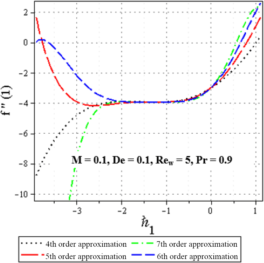
Figure 3 The ℏ₁ – validity for M=0.1, De = 0.1, Re_w = 5 and Pr = 0.9 given by the 4, 5, 6 and 7th-order solution.

Figure 4 The ℏ₂ – validity for M=0, De = 0.3, Re_w = 5 and Pr = 4 given by the 4, 5, 6 and 7th-order solution.

Heat transfer problem

By neglecting viscous and ohmic dissipation, the governing equation of energy obtained is as follows:

$$\begin{array}{}\text{(20)}& {\displaystyle }{u}^{\ast }{\displaystyle \frac{\partial T}{\partial x^{\ast }}}+v^{\ast }{\displaystyle \frac{\partial T}{\partial y^{\ast }}}={\displaystyle \frac{k}{\mathit{\rho }{c}_{\mathrm{p}}}}\left({\displaystyle \frac{{\partial }^{\mathrm{2}}T}{\partial x^{\ast \mathrm{2}}}}+{\displaystyle \frac{{\partial }^{\mathrm{2}}T}{\partial y^{\ast \mathrm{2}}}}\right),\end{array}$$

where T(x,y) is the temperature at any point and k is the thermal conductivity. Similar to the case of channel flow, for the flow of most fluids under practically significant conditions, the following relation holds:

$$\begin{array}{}\text{(21)}& {\displaystyle \frac{{\partial }^{\mathrm{2}}T}{\partial x^{\ast \mathrm{2}}}}\ll {\displaystyle \frac{{\partial }^{\mathrm{2}}T}{\partial y^{\ast \mathrm{2}}}},\end{array}$$

The first term on the right hand side of Eq. (20) can be ignored compared to the second and the energy equation can be approximated as:

$$\begin{array}{}\text{(22)}& {\displaystyle }{u}^{\ast }{\displaystyle \frac{\partial T}{\partial x^{\ast }}}+v^{\ast }{\displaystyle \frac{\partial T}{\partial y^{\ast }}}={\displaystyle \frac{k}{\mathit{\rho }{c}_{\mathrm{p}}}}\left({\displaystyle \frac{{\partial }^{\mathrm{2}}T}{\partial y^{\ast \mathrm{2}}}}\right),\end{array}$$

The flow is assumed to be symmetric, so the appropriate boundary conditions for the above equation are

$$\begin{array}{}\text{(23)}& {\displaystyle }& {\displaystyle }{y}^{\ast }=\mathrm{0}\to {\displaystyle \frac{\partial T}{\partial y^{\ast }}}=\mathrm{0}\text{(24)}& {\displaystyle }& {\displaystyle }{y}^{\ast }=H\to T=T_{\mathrm{w}}\end{array}$$

The non-dimensional variables have been defined as:

$$\begin{array}{}\text{(25)}& {\displaystyle }y={\displaystyle \frac{y^{\ast }}{H}};\mathit{\theta }={\displaystyle \frac{T}{T_{\mathrm{w}}}}\end{array}$$

Inserting the dimensionless parameters described in Eqs. (14) and (25) into the Eqs. (22)–(24) results in:

$$\begin{array}{}\text{(26)}& {\displaystyle }& {\displaystyle }{\mathit{\theta }}^{\prime \prime }-\mathit{\text{Pr}}f\mathit{\theta }=\mathrm{0},\text{(27)}& {\displaystyle }& {\displaystyle }y=\mathrm{1}\to \mathit{\theta }\left(y\right)=\mathrm{1}\text{(28)}& {\displaystyle }& {\displaystyle }y=\mathrm{0}\to {\mathit{\theta }}^{\prime }\left(y\right)=\mathrm{0}\end{array}$$

where $\mathit{\text{Pr}}=\frac{\mathit{\mu }{c}_{\mathrm{p}}}{k}$ represents the Prandtl number.

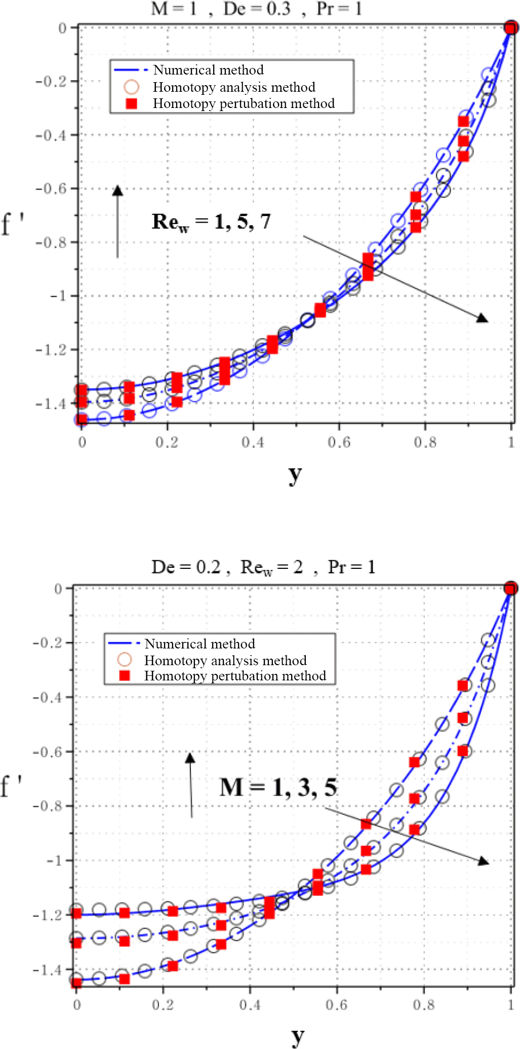
Figure 5 Dimensionless velocities predicted by HAM, HPM and numerical method (NUM) for different Re_w number and De at Pr =1, $\mathrm{\hslash }=-\mathrm{1.5}$.

Figure 6 Effects of De Deborah numbers on the velocity contours for M=1, Pr = 1, Re_w=3.

Figure 7 Effects of M Hartman numbers on the velocity contours for De =0.2, Pr = 1, Re_w=3.

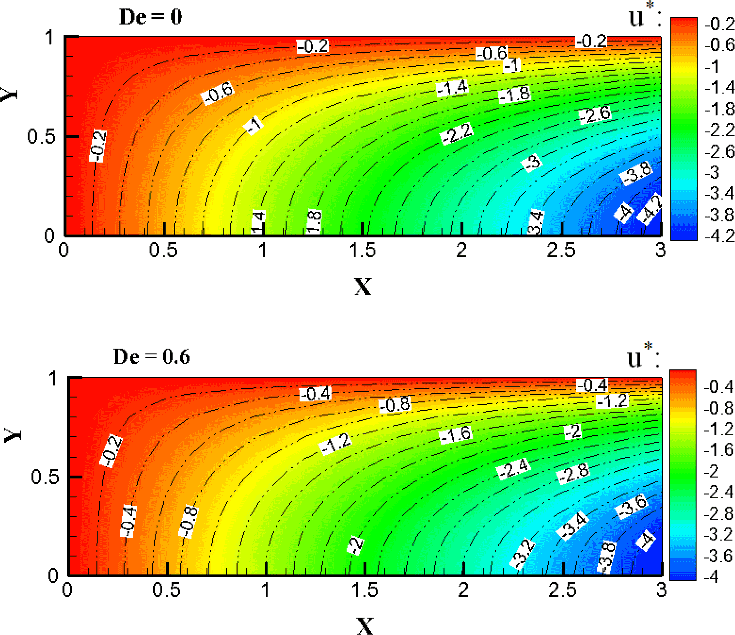
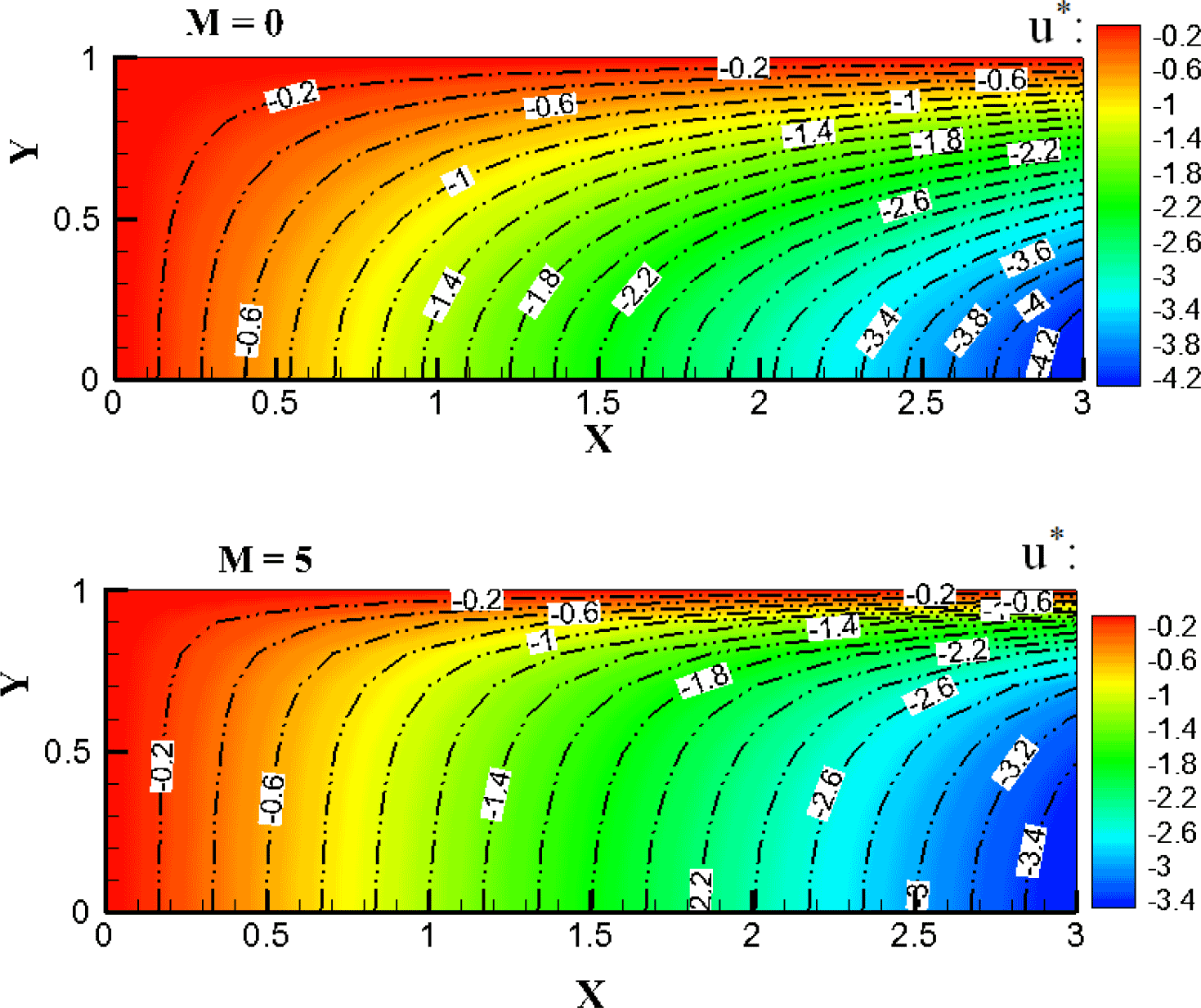
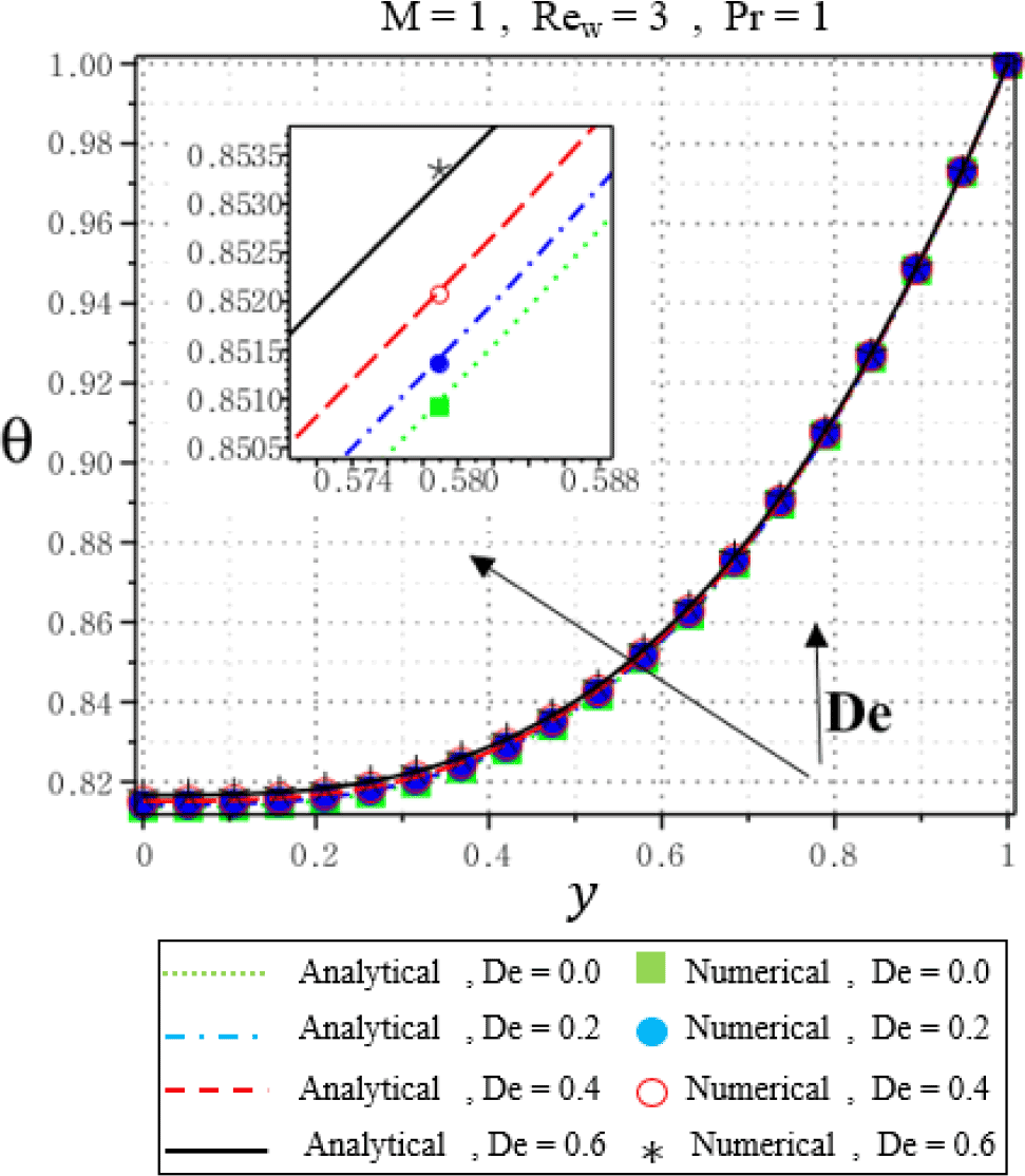
Figure 8 Dimensionless temperature predicted by analytical and numerical method (NUM) for different De Deborah number at M=1, Re_w=3, Pr = 1, $\mathrm{\hslash }=-\mathrm{1.5}$.

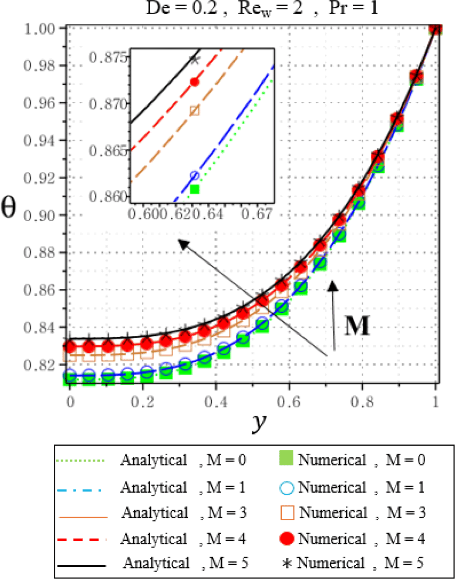
Figure 9 Dimensionless temperature predicted by analytical and numerical method (NUM) for different M Hartman number at De = 0.2, Re_w=2, Pr = 1, $\mathrm{\hslash }=-\mathrm{1}$.

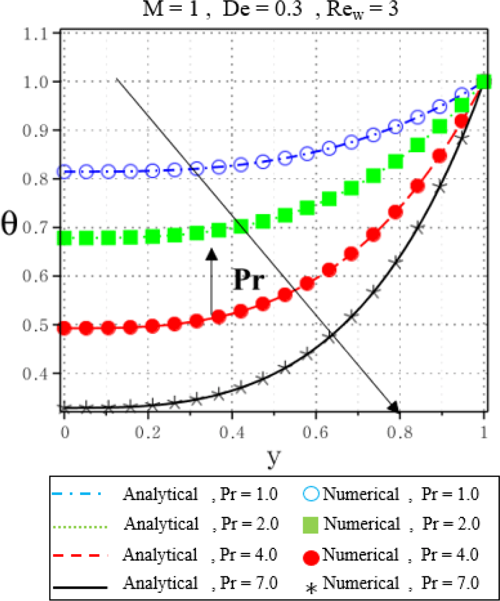
Figure 10 Dimensionless temperature predicted by analytical and numerical method (NUM) for different Pr Prandtl number at M=1, Re_w=3, De = 0.3, $\mathrm{\hslash }=-\mathrm{1}$.

3 Analytical methods

3.1 Implementation of the Homotopy Perturbation Method

In this section, we employ HPM to solve Eq. (2) subject to the boundary conditions Eq. (3). One can construct the Homotopy function of Eq. (2) as described in (He, 2000):

$$\begin{array}{ll}{\displaystyle }& {\displaystyle }H\left(f,p\right)=\left(\mathrm{1}-P\right)\left[f{}^{\prime \prime \prime \prime }\left(\mathit{\eta }\right)-g_{\mathrm{0}}\left(y\right)\right]+p\left\{f^{\prime \prime \prime \prime }-M^{\mathrm{2}}{f}^{\prime \prime }\right.\\ {\displaystyle }& {\displaystyle }+{\mathit{\text{Re}}}_{\mathrm{w}}\left(f^{\prime }{f}^{\prime \prime }-f{f}^{\prime \prime \prime }\right)\\ \text{(29)}& {\displaystyle }& {\displaystyle }\left.\mathit{\text{De}}\left(\mathrm{2}{f^{\prime }}^{\mathrm{2}}{f}^{\prime \prime }+\mathrm{2}f{f^{\prime \prime }}^{\mathrm{2}}-f^{\mathrm{2}}{f}^{\prime \prime \prime \prime }\right)\right\}=\mathrm{0},{\displaystyle }& {\displaystyle }H\left(\mathit{\theta },p\right)=\left(\mathrm{1}-P\right)\left[{\mathit{\theta }}^{\prime \prime }\left(y\right)-g_{\mathrm{0}}\left(y\right)\right]\\ \text{(30)}& {\displaystyle }& {\displaystyle }+p\left[{\mathit{\theta }}^{\prime \prime }-\mathit{\text{Pr}}f\mathit{\theta }\right]=\mathrm{0},\end{array}$$

where $p\in \left[\mathrm{0},\mathrm{1}\right]$ is an embedded parameter. For p=0 and p=1 one has:

$$\begin{array}{ll}{\displaystyle }& {\displaystyle }f\left(y,\mathrm{0}\right)=f_{\mathrm{0}}\left(y\right),f\left(y,\mathrm{1}\right)=f\left(y\right)\\ \text{(31)}& {\displaystyle }& {\displaystyle }\mathit{\theta }\left(y,\mathrm{0}\right)={\mathit{\theta }}_{\mathrm{0}}\left(y\right),\mathit{\theta }\left(y,\mathrm{1}\right)=\mathit{\theta }\left(y\right)\end{array}$$

Note that when p increases from 0 to 1, f(y  , p), θ(y,p) varies from f₀(y), θ₀(y) to f(y), θ(y).

$$\begin{array}{ll}{\displaystyle }& {\displaystyle }f\left(y\right)=f_{\mathrm{0}}\left(y\right)+p{f}_{\mathrm{1}}\left(y\right)+p^{\mathrm{2}}{f}_{\mathrm{2}}\left(y\right)+\mathrm{\dots }\\ {\displaystyle }& {\displaystyle }=\sum _{i=\mathrm{0}}^n{p}^i{f}_i\left(y\right),g_{\mathrm{0}}=\mathrm{0}\\ {\displaystyle }& {\displaystyle }\mathit{\theta }\left(y\right)={\mathit{\theta }}_{\mathrm{0}}\left(y\right)+p{\mathit{\theta }}_{\mathrm{1}}\left(\mathit{\eta }\right)+p^{\mathrm{2}}{\mathit{\theta }}_{\mathrm{2}}\left(y\right)+\mathrm{\dots }\\ \text{(32)}& {\displaystyle }& {\displaystyle }=\sum _{i=\mathrm{0}}^n{p}^i{\mathit{\theta }}_i\left(y\right),g_{\mathrm{0}}=\mathrm{0}\end{array}$$

By substitution of Eq. (32) into the Eqs. (18) and (26), rearranging based on powers of p-terms and solving these equations result in the following terms:

$$\begin{array}{ll}\text{(33)}& {\displaystyle }& {\displaystyle }{f}_{\mathrm{0}}\left(y\right)=\mathrm{0.5}{y}^{\mathrm{3}}-\mathrm{1.5}{y}^{\mathrm{2}},{\displaystyle }& {\displaystyle }{f}_{\mathrm{1}}\left(y\right)=\mathrm{0.007440476190}\mathit{\text{De}}{y}^{\mathrm{9}}\\ {\displaystyle }& {\displaystyle }-\mathrm{0.001785714286}\left(\mathrm{36}.+\mathrm{2.0}{\mathit{\text{Re}}}_{\mathrm{w}}\right)y^{\mathrm{7}}\\ {\displaystyle }& {\displaystyle }-\mathrm{0.0125000}\left(\mathrm{2.0}{M}^{\mathrm{2}}-\mathrm{9}.\right)y^{\mathrm{5}}\\ {\displaystyle }& {\displaystyle }+\mathrm{0.1666666667}\left(\mathrm{0.300}{M}^{\mathrm{2}}-\mathrm{0.3714285714}\right.\\ {\displaystyle }& {\displaystyle }\left.+\mathrm{0.06428571429}{\mathit{\text{Re}}}_{\mathrm{w}}\right)y^{\mathrm{3}}\\ \text{(34)}& {\displaystyle }& {\displaystyle }+\left(-\mathrm{0.025}{M}^{\mathrm{2}}+\mathrm{0.00625}-\mathrm{0.007142857143}{\mathit{\text{Re}}}_{\mathrm{w}}\right)y{\displaystyle }& {\displaystyle }{f}_{\mathrm{2}}\left(y\right)=-\mathrm{0.000040881}{\mathit{\text{De}}}^{\mathrm{2}}{x}^{\mathrm{15}}-{\mathrm{1.16550116610}}^{-\mathrm{25}}\\ {\displaystyle }& {\displaystyle }\left(-{\mathrm{3.013392810}}^{\mathrm{21}}{\mathit{\text{De}}}^{\mathrm{2}}-{\mathrm{2.23214210}}^{\mathrm{20}}{\mathit{\text{DeRe}}}_{\mathrm{w}}\right)x^{\mathrm{13}}\\ {\displaystyle }& {\displaystyle }-{\mathrm{2.52525210}}^{-\mathrm{25}}\left(-{\mathrm{3.8678510}}^{\mathrm{21}}{\mathit{\text{DeM}}}^{\mathrm{2}}-{\mathrm{7.907110}}^{\mathrm{21}}{\mathit{\text{De}}}^{\mathrm{2}}\right.\\ {\displaystyle }& {\displaystyle }\left.-{\mathrm{3.18214210}}^{\mathrm{21}}{\mathit{\text{DeRe}}}_{\mathrm{w}}-{\mathrm{4.2857110}}^{\mathrm{19}}{\mathit{\text{Re}}}_{\mathrm{w}}^{\mathrm{2}}\right)x^{\mathrm{11}}\\ {\displaystyle }& {\displaystyle }-{\mathrm{6.61375661410}}^{-\mathrm{25}}\left(\begin{array}{l}{\mathrm{1.035010}}^{\mathrm{22}}{\mathit{\text{DeM}}}^{\mathrm{2}}+{\mathrm{2.2510}}^{\mathrm{20}}{M}^{\mathrm{2}}{\mathit{\text{Re}}}_{\mathrm{w}}\\ +{\mathrm{2.518310}}^{\mathrm{22}}{\mathit{\text{De}}}^{\mathrm{2}}+{\mathrm{1.11810}}^{\mathrm{22}}\mathit{\text{De}}{\mathit{\text{Re}}}_{\mathrm{w}}\\ +{\mathrm{4.5010}}^{\mathrm{20}}{\mathit{\text{Re}}}_{\mathrm{w}}^{\mathrm{2}}\end{array}\right)x^{\mathrm{9}}\\ {\displaystyle }& {\displaystyle }-{\mathrm{2.38095230110}}^{-\mathrm{24}}\left(\begin{array}{l}-{\mathrm{4.72510}}^{\mathrm{21}}{\mathit{\text{DeM}}}^{\mathrm{2}}+{\mathrm{4.510}}^{\mathrm{20}}{M}^{\mathrm{2}}{\mathit{\text{Re}}}_{\mathrm{w}}\\ -{\mathrm{3.326710}}^{\mathrm{21}}{\mathit{\text{De}}}^{\mathrm{2}}-{\mathrm{4.28928410}}^{\mathrm{21}}{\mathit{\text{DeRe}}}_{\mathrm{w}}\\ -{\mathrm{6.42857143010}}^{\mathrm{19}}{\mathit{\text{Re}}}^{\mathrm{2}}+{\mathrm{2.510}}^{\mathrm{20}}{M}^{\mathrm{4}}\end{array}\right)x^{\mathrm{7}}\\ {\displaystyle }& {\displaystyle }-{\mathrm{1.6666710}}^{-\mathrm{23}}\left(-{\mathrm{1.5010}}^{\mathrm{20}}{M}^{\mathrm{4}}+{\mathrm{1.0854210}}^{\mathrm{21}}{\mathit{\text{DeM}}}^{\mathrm{2}}\right.\\ {\displaystyle }& {\displaystyle }\left.-{\mathrm{3.214257710}}^{\mathrm{19}}{M}^{\mathrm{2}}{\mathit{\text{Re}}}_{\mathrm{w}}-{\mathrm{8.91987910}}^{\mathrm{20}}{\mathit{\text{De}}}^{\mathrm{2}}+\right)x^{\mathrm{5}}\\ {\displaystyle }& {\displaystyle }\mathrm{0.166666666}\left(\begin{array}{l}-\mathrm{0.019285}{M}^{\mathrm{4}}+\mathrm{0.14962}{\mathit{\text{DeM}}}^{\mathrm{2}}+\mathrm{0.0164}{M}^{\mathrm{2}}{\mathit{\text{Re}}}_{\mathrm{w}}\\ +\mathrm{0.007946}{\mathit{\text{De}}}^{\mathrm{2}}+\mathrm{0.0104}{\mathit{\text{DeRe}}}_{\mathrm{w}}\\ +\mathrm{0.0040630}{\mathit{\text{Re}}}_{\mathrm{w}}^{\mathrm{2}}\end{array}\right)x^{\mathrm{3}}\\ {\displaystyle }& {\displaystyle }+\left(\mathrm{0.001309}{M}^{\mathrm{4}}-\mathrm{0.0122}\mathit{\text{De}}{M}^{\mathrm{2}}\right.\\ {\displaystyle }& {\displaystyle }-\mathrm{0.002053}{M}^{\mathrm{2}}{\mathit{\text{Re}}}_{\mathrm{w}}-\mathrm{0.009762}{\mathit{\text{De}}}^{\mathrm{2}}\\ \text{(35)}& {\displaystyle }& {\displaystyle }\left.-\mathrm{0.001906}\mathit{\text{DeRe}}-\mathrm{0.00054}{\mathit{\text{Re}}}_{\mathrm{w}}^{\mathrm{2}}\right)x{\displaystyle }& {\displaystyle }\mathrm{⋮}\\ \text{(36)}& {\displaystyle }& {\displaystyle }{\mathit{\theta }}_{\mathrm{0}}\left(y\right)=\mathrm{1}\text{(37)}& {\displaystyle }& {\displaystyle }{\mathit{\theta }}_{\mathrm{1}}\left(y\right)=-\mathrm{0.025}\mathit{\text{Pr}}{y}^{\mathrm{5}}+\mathrm{0.25}\mathit{\text{Pr}}{y}^{\mathrm{3}}-\mathrm{0.225}\mathit{\text{Pr}}{\displaystyle }& {\displaystyle }{\mathit{\theta }}_{\mathrm{2}}\left(y\right)=\mathrm{0.0000676}\\ {\displaystyle }& {\displaystyle }\mathit{\text{Pr}}\mathit{\text{De}}{y}^{\mathrm{11}}+\mathrm{0.0001388}{\mathit{\text{Pr}}}^{\mathrm{2}}{y}^{\mathrm{10}}-\mathrm{0.00089283}\mathit{\text{Pr}}\mathit{\text{De}}{y}^{\mathrm{9}}\\ {\displaystyle }& {\displaystyle }-\mathrm{0.000049603}\mathit{\text{Pr}}{x}^{\mathrm{9}}{\mathit{\text{Re}}}_{\mathrm{w}}\\ {\displaystyle }& {\displaystyle }-\mathrm{0.00285714}{y}^{\mathrm{8}}{\mathit{\text{Pr}}}^{\mathrm{2}}-\mathrm{0.000595552}\mathit{\text{Pr}}{x}^{\mathrm{7}}{M}^{\mathrm{2}}\\ {\displaystyle }& {\displaystyle }+\mathrm{0.002645789}\mathit{\text{Pr}}\mathit{\text{De}}{y}^{\mathrm{7}}-\mathrm{0.0030959651}\mathit{\text{Pr}}\mathit{\text{De}}{y}^{\mathrm{5}}\\ {\displaystyle }& {\displaystyle }+\mathrm{0.01250000}{x}^{\mathrm{6}}{\mathit{\text{Pr}}}^{\mathrm{2}}+\mathrm{0.00250000}\mathit{\text{Pr}}{x}^{\mathrm{5}}{M}^{\mathrm{2}}\\ {\displaystyle }& {\displaystyle }+\mathrm{0.00562544000}{y}^{\mathrm{5}}{\mathit{\text{Pr}}}^{\mathrm{2}}+\mathrm{0.0010467104}\mathit{\text{Pr}}\mathit{\text{De}}{y}^{\mathrm{3}}\\ {\displaystyle }& {\displaystyle }\mathrm{0.000535}\mathit{\text{Pr}}{y}^{\mathrm{5}}{\mathit{\text{Re}}}_{\mathrm{w}}-\mathrm{0.004167}\mathit{\text{Pr}}{M}^{\mathrm{2}}{y}^{\mathrm{3}}\\ {\displaystyle }& {\displaystyle }-\mathrm{0.05625}{\mathit{\text{Pr}}}^{\mathrm{2}}{y}^{\mathrm{3}}+\mathrm{0.000200507}\mathit{\text{Pr}}\mathit{\text{De}}\\ {\displaystyle }& {\displaystyle }+\mathrm{0.0408878}{\mathit{\text{Pr}}}^{\mathrm{2}}\\ {\displaystyle }& {\displaystyle }-\mathrm{0.001190470}\mathit{\text{Pr}}{\mathit{\text{Re}}}_{\mathrm{w}}{y}^{\mathrm{3}}+\mathrm{0.0022619}\mathit{\text{Pr}}{M}^{\mathrm{2}}\\ \text{(38)}& {\displaystyle }& {\displaystyle }+\mathrm{0.000703}\mathit{\text{Pr}}{\mathit{\text{Re}}}_{\mathrm{w}}{\displaystyle }& {\displaystyle }\mathrm{⋮}\end{array}$$

The solution of this equation, when p→1, is as follows:

$$\begin{array}{}\text{(39)}& {\displaystyle }& {\displaystyle }f\left(y\right)=\sum _{i=\mathrm{0}}^{\mathrm{9}}{\mathrm{Lim}}_{p\to \mathrm{1}}{p}^i{f}_i\left(y\right)\text{(40)}& {\displaystyle }& {\displaystyle }\mathit{\theta }\left(y\right)=\sum _{i=\mathrm{0}}^{\mathrm{9}}{\mathrm{Lim}}_{p\to \mathrm{1}}{p}^i{\mathit{\theta }}_i\left(y\right)\end{array}$$

3.2 Implementation of the Homotopy Analysis Method

For HAM solutions, the auxiliary linear operators are chosen in the following form:

$$\begin{array}{}\text{(41)}& {\displaystyle }& {\displaystyle }L\left(f\right)=f^{\prime \prime \prime \prime },\text{(42)}& {\displaystyle }& {\displaystyle }L\left(\mathit{\theta }\right)={\mathit{\theta }}^{\prime \prime },\end{array}$$

The initially guessed function is obtained by solving the following equations:

$$\begin{array}{}\text{(43)}& {\displaystyle }& {\displaystyle }L({\displaystyle \frac{\mathrm{1}}{\mathrm{6}}}{c}_{\mathrm{1}}{y}^{\mathrm{3}}+{\displaystyle \frac{\mathrm{1}}{\mathrm{2}}}{c}_{\mathrm{2}}{y}^{\mathrm{2}}+c_{\mathrm{3}}y+c_{\mathrm{4}})=\mathrm{0},\text{(44)}& {\displaystyle }& {\displaystyle }L(c_{\mathrm{5}}y+c_{\mathrm{6}})=\mathrm{0},\end{array}$$

with boundary Eqs. (17), (27) and (28) as:

$$\begin{array}{}\text{(45)}& {\displaystyle }& {\displaystyle }{f}_{\mathrm{0}}\left(y\right)=-{\displaystyle \frac{\mathrm{1}}{\mathrm{2}}}{y}^{\mathrm{3}}+{\displaystyle \frac{\mathrm{3}}{\mathrm{2}}}y,\text{(46)}& {\displaystyle }& {\displaystyle }{\mathit{\theta }}_{\mathrm{0}}\left(y\right)=\mathrm{1},\end{array}$$

Let $P\in \left[\mathrm{0},\mathrm{1}\right]$ denote the embedded parameter and ℏ indicate non–zero auxiliary parameters. Consequently the following equations are constructed.

Zeroth – order deformation equations

$$\begin{array}{ll}\text{(47)}& {\displaystyle }& {\displaystyle }(\mathrm{1}-P)L\left[F(y;p)-f_{\mathrm{0}}\left(y\right)\right]=p\mathrm{\hslash }H\left(y\right)N\left[F(y;p)\right]\text{(48)}& {\displaystyle }& {\displaystyle }(\mathrm{1}-P)L\left[\mathrm{\Theta }(y;p)-{\mathit{\theta }}_{\mathrm{0}}\left(y\right)\right]=p\mathrm{\hslash }H\left(y\right)N\left[\mathrm{\Theta }(y;p)\right]{\displaystyle }& {\displaystyle }F(\mathrm{0};p)=\mathrm{1};F^{\prime \prime }(\mathrm{0};p)=\mathrm{0},\\ \text{(49)}& {\displaystyle }& {\displaystyle }F(\mathrm{1};p)=\mathrm{1},F^{\prime }(\mathrm{1};p)=\mathrm{0}\text{(50)}& {\displaystyle }& {\displaystyle }\mathit{\theta }(\mathrm{1};p)=\mathrm{1};{\mathit{\theta }}^{\prime }(\mathrm{0};p)=\mathrm{0}{\displaystyle }& {\displaystyle }N\left[F\right(y;p\left)\right]={\displaystyle \frac{{\mathrm{d}}^{\mathrm{4}}F(y;p)}{\mathrm{d}{y}^{\mathrm{4}}}}\\ {\displaystyle }& {\displaystyle }+\mathit{\text{Re}}\left[{\displaystyle \frac{\mathrm{d}F(y;p)}{\mathrm{d}y}}{\displaystyle \frac{{\mathrm{d}}^{\mathrm{2}}F(y;p)}{\mathrm{d}{y}^{\mathrm{2}}}}\right.\\ {\displaystyle }& {\displaystyle }\left.-F(y;p){\displaystyle \frac{{\mathrm{d}}^{\mathrm{3}}F(y;p)}{\mathrm{d}{y}^{\mathrm{3}}}}\right]\\ {\displaystyle }& {\displaystyle }+\mathit{\text{De}}\left[\mathrm{2}{\left({\displaystyle \frac{\mathrm{d}F(y;p)}{\mathrm{d}y}}\right)}^{\mathrm{2}}{\displaystyle \frac{{\mathrm{d}}^{\mathrm{2}}F(y;p)}{\mathrm{d}{y}^{\mathrm{2}}}}\right.\\ {\displaystyle }& {\displaystyle }\left.-\mathrm{2}F(y;p){\left({\displaystyle \frac{{\mathrm{d}}^{\mathrm{2}}F(y;p)}{\mathrm{d}{y}^{\mathrm{2}}}}\right)}^{\mathrm{2}}-F(y;p{)}^{\mathrm{2}}{\displaystyle \frac{{\mathrm{d}}^{\mathrm{4}}F(y;p)}{\mathrm{d}{y}^{\mathrm{4}}}}\right]\\ \text{(51)}& {\displaystyle }& {\displaystyle }+\left(M^{\mathrm{2}}\right){\displaystyle \frac{{\mathrm{d}}^{\mathrm{2}}F(y;p)}{\mathrm{d}{y}^{\mathrm{2}}}}\text{(52)}& {\displaystyle }& {\displaystyle }N\left[\mathit{\theta }\right(y;p\left)\right]={\displaystyle \frac{{\mathrm{d}}^{\mathrm{2}}\mathit{\theta }(y;p)}{\mathrm{d}{y}^{\mathrm{2}}}}+\mathit{\text{Pr}}F(y;p){\displaystyle \frac{\mathrm{d}\mathit{\theta }(y;p)}{\mathrm{d}y}}\end{array}$$

For p=0 and p=1, one has:

$$\begin{array}{}\text{(53)}& {\displaystyle }& {\displaystyle }F(y;\mathrm{0})=f_{\mathrm{0}}\left(y\right)F(y;\mathrm{1})=f\left(y\right)\text{(54)}& {\displaystyle }& {\displaystyle }\mathit{\theta }(y;\mathrm{0})={\mathit{\theta }}_{\mathrm{0}}\left(y\right)\mathit{\theta }(y;\mathrm{1})=\mathit{\theta }\left(y\right)\end{array}$$

As p increases from 0 to 1 then F(y;p), θ(y;p) varies from f₀(y), θ₀(y) to f(y), θ(y). By Taylor's theorem, F(y;p), θ(y;p) can be expanded in a power series of p as follows:

$$\begin{array}{ll}{\displaystyle }& {\displaystyle }F(y;p)=f_{\mathrm{0}}\left(y\right)+\sum _{m-\mathrm{1}}^{\mathrm{\infty }}{f}_{\mathrm{m}}\left(y\right)p^m\\ \text{(55)}& {\displaystyle }& {\displaystyle }{f}_{\mathrm{m}}\left(y\right)={\left.{\displaystyle \frac{\mathrm{1}}{m}}{\displaystyle \frac{{\partial }^m\left(F\right(y;p\left)\right)}{\partial p^m}}\right|}_{p=\mathrm{0}}{\displaystyle }& {\displaystyle }\mathit{\theta }(y;p)={\mathit{\theta }}_{\mathrm{0}}\left(y\right)+\sum _{m-\mathrm{1}}^{\mathrm{\infty }}{\mathit{\theta }}_{\mathrm{m}}\left(y\right)p^m\\ \text{(56)}& {\displaystyle }& {\displaystyle }{\mathit{\theta }}_{\mathrm{m}}\left(y\right)={\left.{\displaystyle \frac{\mathrm{1}}{m}}{\displaystyle \frac{{\partial }^m\left(\mathit{\theta }\right(y;p\left)\right)}{\partial p^m}}\right|}_{p=\mathrm{0}}\end{array}$$

there ℏ is chosen in such a way that this series is convergent at p=1, therefore through Eqs. (55) and (56), it can be concluded that:

$$\begin{array}{}\text{(57)}& {\displaystyle }& {\displaystyle }f\left(y\right)=f_{\mathrm{0}}\left(y\right)+\sum _{m-\mathrm{1}}^{\mathrm{\infty }}{f}_{\mathrm{m}}\left(y\right),\text{(58)}& {\displaystyle }& {\displaystyle }\mathit{\theta }\left(y\right)={\mathit{\theta }}_{\mathrm{0}}\left(y\right)+\sum _{m-\mathrm{1}}^{\mathrm{\infty }}{\mathit{\theta }}_{\mathrm{m}}\left(y\right),\end{array}$$

mth – order deformation equations

The mth-order deformation equations are written as:

$$\begin{array}{ll}\text{(59)}& {\displaystyle }& {\displaystyle }L\left[f_{\mathrm{m}}\left(y\right)-{\mathit{\chi }}_{\mathrm{m}}{f}_{m-\mathrm{1}}\left(y\right)\right]=\mathrm{\hslash }H\left(y\right)R_{\mathrm{m}}^f\left(y\right)\text{(60)}& {\displaystyle }& {\displaystyle }L\left[{\mathit{\theta }}_{\mathrm{m}}\left(y\right)-{\mathit{\chi }}_{\mathrm{m}}{\mathit{\theta }}_{m-\mathrm{1}}\left(y\right)\right]=\mathrm{\hslash }H\left(y\right)R_{\mathrm{m}}^{\mathit{\theta }}\left(y\right){\displaystyle }& {\displaystyle }{F}_{\mathrm{m}}(\mathrm{0};p)=\mathrm{0};F_{\mathrm{m}}^{\prime \prime }(\mathrm{0};p)=\mathrm{0},\\ \text{(61)}& {\displaystyle }& {\displaystyle }{F}_{\mathrm{m}}(\mathrm{1};p)=\mathrm{0},F_{\mathrm{m}}^{\prime }(\mathrm{1};p)=\mathrm{0}\text{(62)}& {\displaystyle }& {\displaystyle }{\mathit{\theta }}_{\mathrm{m}}(\mathrm{1};p)=\mathrm{0};{\mathit{\theta }}_{\mathrm{m}}^{\prime }(\mathrm{0};p)=\mathrm{0}{\displaystyle }& {\displaystyle }{R}_{\mathrm{m}}^f\left(y\right)={f^{\prime \prime }}_{m-\mathrm{1}}^{\prime \prime }+\sum _{k=\mathrm{0}}^{m-\mathrm{1}}\left[\mathit{\text{Re}}\left(f_{m-\mathrm{1}-k}^{\prime }{f}_k^{\prime \prime }-f_{m-\mathrm{1}-k}{f}_k^{\prime \prime \prime }\right)\right.\\ {\displaystyle }& {\displaystyle }+\mathit{\text{De}}{f}_{m-\mathrm{1}-k}^{\prime }\left(\sum _{l=\mathrm{0}}^k\left(\mathrm{2}{f}_{k-l}^{\prime }{f}_l^{\prime \prime }\right)\right)\\ {\displaystyle }& {\displaystyle }\left.-\mathit{\text{De}}{f}_{m-\mathrm{1}-k}\left(\sum _{l=\mathrm{0}}^k\left(\mathrm{2}{f}_{k-l}^{\prime \prime }{f}_l^{\prime \prime }+f_{k-l}{f}_l^{\prime \prime \prime \prime }\right)\right)\right]\\ \text{(63)}& {\displaystyle }& {\displaystyle }+\left(M^{\mathrm{2}}\right)f_{m-\mathrm{1}}^{\prime \prime }\text{(64)}& {\displaystyle }& {\displaystyle }{R}_{\mathrm{m}}^{\mathit{\theta }}\left(y\right)={\mathit{\theta }}_{m-\mathrm{1}}^{\prime \prime }-\sum _{k=\mathrm{0}}^{m-\mathrm{1}}\left[\mathit{\text{Pr}}\left(f_{m-\mathrm{1}-k}{\mathit{\theta }}_k^{\prime }\right)\right]\text{(65)}& {\displaystyle }& {\displaystyle }{\mathit{\chi }}_{\mathrm{m}}=\left\{\begin{array}{l}\mathrm{0},m\le \mathrm{1}\\ \mathrm{1},m>\mathrm{1}\end{array}\right.\end{array}$$

For simplicity, it is assumed that:

$$\begin{array}{}\text{(66)}& {\displaystyle }H\left(y\right)=\mathrm{1}\end{array}$$

For different values of m, the solution is obtained by maple analytic solution device. The first deformation is presented as:

$$\begin{array}{ll}{\displaystyle }& {\displaystyle }{f}_{\mathrm{1}}\left(y\right)=-{\displaystyle \frac{\mathrm{5}}{\mathrm{672}}}{\mathrm{\hslash }}_{\mathrm{1}}\mathit{\text{De}}{y}^{\mathrm{9}}-{\displaystyle \frac{\mathrm{3}}{\mathrm{2}}}{\mathrm{\hslash }}_{\mathrm{1}}\left(-{\displaystyle \frac{\mathrm{1}}{\mathrm{420}}}{\mathit{\text{Re}}}_{\mathrm{w}}-{\displaystyle \frac{\mathrm{3}}{\mathrm{70}}}\mathit{\text{De}}\right)y^{\mathrm{7}}\\ {\displaystyle }& {\displaystyle }-{\displaystyle \frac{\mathrm{3}}{\mathrm{2}}}{\mathrm{\hslash }}_{\mathrm{1}}\left({\displaystyle \frac{\mathrm{3}}{\mathrm{40}}}B-{\displaystyle \frac{\mathrm{1}}{\mathrm{60}}}{M}^{\mathrm{2}}\right)y^{\mathrm{5}}\\ {\displaystyle }& {\displaystyle }+\left({\displaystyle \frac{\mathrm{13}}{\mathrm{210}}}{\mathrm{\hslash }}_{\mathrm{1}}\mathit{\text{De}}-{\displaystyle \frac{\mathrm{3}}{\mathrm{280}}}{\mathrm{\hslash }}_{\mathrm{1}}{\mathit{\text{Re}}}_{\mathrm{w}}-{\displaystyle \frac{\mathrm{1}}{\mathrm{20}}}{\mathrm{\hslash }}_{\mathrm{1}}{M}^{\mathrm{2}}\right)y^{\mathrm{3}}\\ \text{(67)}& {\displaystyle }& {\displaystyle }+\left(-{\displaystyle \frac{\mathrm{1}}{\mathrm{160}}}{\mathrm{\hslash }}_{\mathrm{1}}\mathit{\text{De}}+{\displaystyle \frac{\mathrm{1}}{\mathrm{140}}}{\mathrm{\hslash }}_{\mathrm{1}}{\mathit{\text{Re}}}_{\mathrm{w}}+{\displaystyle \frac{\mathrm{1}}{\mathrm{40}}}{h}_{\mathrm{1}}{M}^{\mathrm{2}}\right)y\text{(68)}& {\displaystyle }& {\displaystyle }{\mathit{\theta }}_{\mathrm{1}}\left(y\right)={\displaystyle \frac{\mathrm{1}}{\mathrm{40}}}{\mathrm{\hslash }}_{\mathrm{2}}\mathit{\text{Pr}}{y}^{\mathrm{5}}-{\displaystyle \frac{\mathrm{1}}{\mathrm{4}}}{\mathrm{\hslash }}_{\mathrm{2}}\mathit{\text{Pr}}{y}^{\mathrm{3}}+{\displaystyle \frac{\mathrm{9}}{\mathrm{40}}}{\mathrm{\hslash }}_{\mathrm{2}}\mathit{\text{Pr}}\end{array}$$

The solutions of f(y),θ(y) are too long and will be shown in obtained results.

3.2.1 Convergence of the HAM solution

As pointed out by Liao (2012), the convergence region and rate of solution series can be adjusted and controlled by means of the auxiliary parameter ℏ. In order to check the convergence of the present solution, the so-called ℏ₁-curve of f^′′(1) is depicted in Figs. 2 and 3 and the ℏ₂-curve of θ^′(1) is shown in Fig. 4.

The solutions converge for ℏ values which correspond to the horizontal line segment in the ℏ curve. In order to investigate the range of admissible values of the auxiliary parameter ℏ, the ℏ-curve of f^′′(1) is illustrated for various quantities of De, M and Re_w in Fig. 3. Similarly, the ℏ₂-curve of θ^′(1) is shown in Fig. 4. As seen clearly in Figs. 2–4, it can be concluded that ${\mathrm{\hslash }}_{\mathrm{1}}={\mathrm{\hslash }}_{\mathrm{2}}=-\mathrm{1}$ are suitable values for different quantities within $\mathrm{0.1}<\mathit{\text{De}}<\mathrm{0.6}$, $\mathrm{0}<M<\mathrm{5}$ and $-\mathrm{5}<{\mathit{\text{Re}}}_{\mathrm{w}}<\mathrm{5}(\le T\le \mathrm{6})$.

4 Numerical method

The above system of non-linear ordinary differential Eqs. (17) and (23) along with the boundary conditions (16), (24) and (25) are solved numerically using the algebra package Maple 16.0. The package uses a boundary value (B-V) problem procedure. The algorithm can be used to find moderate accurate solutions for ODE boundary and initial value problems, both with a global error bound. The method uses either Richardson extrapolation or deferred corrections with a base method of either the trapezoid or midpoint method. The trapezoid method is generally efficient for typical problems, while the midpoint method is a powerful method for solving harmless end-point singularities that the trapezoid method cannot. The midpoint method, also known as the fourth-order Runge–Kutta–Fehlberg method, improves the Euler method by adding a midpoint in the step which increases the accuracy by one order. Thus, the midpoint method is used as a suitable numerical technique (Hatami et al., 2013; Aziz, 2006).

5 Results and discussion

In the present study HAM and HPM methods are applied to obtain an explicit analytic solution of the MHD flow of an UCM fluid in a channel (Fig. 1). Comparison between the results obtained by the numerical method (Runge-Kutta-Fehlberg technique), Homotopy Perturbation and Homotopy Analysis Methods for different values of active parameters is shown in Fig. 5. The results are proved to be precise and accurate in solving a wide range of mathematical and engineering problems especially Fluid mechanics cases. This investigation is completed by depicting the effects of some important parameters to determine how these parameters affect the fluid flow and heat transfer. From a physical point of view, Figs. 6–10 are presented in order to highlight the effects of the Deborah number De, Hartman number M and Prandtl number Pr on the velocity and temperature profiles.

Figure 6 shows the effect of Deborah number on the velocity distribution for M=1, Pr =1, Re_w=3. This number may be interpreted as the ratio of the relaxation time, and the characteristic time of an experiment or a computer simulation probing the response of the material (Reiner, 1964). Higher De values imply a strongly elastic behavior. The Newtonian fluids possess no relaxation time (i.e., De = 0). An increase in the elastic parameter (i.e. as De rises from 0 to 0.6) results in a decrease of the velocity components at any given point (Hayat et al., 2009; Mostafa and Mahmoud, 2011). Figure 7 shows the effect of a Hartman number M on the velocity components for De =0.2, Pr =1, Re_w=3. An increase of the magnetic parameter leads to a decrease in the velocity components and contours at a given point. This is due to the fact that the applied transverse magnetic field produces damping in form of a Lorentz force thereby decreasing the magnitude of the velocity. The drop in velocity as a consequence of an increase in the strength of the magnetic field is observed.

Figures 8 show the variation of temperature for different values of the viscoelastic parameter Deborah number De. From Fig. 8, it is found that the temperature field increases with an increase of the Deborah number De. It is remarkable to note that, since the Deborah number has depended on the relaxation time, the larger values of Deborah number imply to higher relaxation time. It is well known fact that the larger relaxation time fluids leads to a higher temperature (Khan et al., 2016).

Also, the effects of Hartman parameter M on the temperature profile have been illustrated in Fig. 9. It can be inferred from this figure that the temperature increases with an increase in the magnetic field. Application of a magnetic field normal to an electrically conducting fluid has the tendency to produce a resistive type of body force called the Lorentz force which opposes the fluid motion, causing a flow retardation effect. This causes the fluid velocity to decrease. However, this decrease in flow speed is accompanied by corresponding increases in the fluid thermal state level (Mostafa and Mahmoud, 2011). This can be attributed to the fact that, u is small and an increase in Ha increases the Joule dissipation which is proportional to Ha and therefore, the temperature increases.

Figure 10 shows the effect of Prandtl number on the dimensionless temperature profile. As observed, an increase in the Prandtl number leads to a decrease in the temperature. This is in agreement with the physical fact that the thermal boundary layer thickness decreases with increasing Pr.

6 Conclusions

In this investigation, the analytical approaches called Homotopy Analysis Method (HAM), Homotopy Perturbation Method (HPM) have been successfully applied to find the most accurate analytical solution for the velocity and temperature distributions of MHD flow of an upper-convected Maxwell fluid in a channel. Furthermore, the obtained solutions by the proposed method have been compared with the direct numerical solutions using the Runge-Kutta-Fehlberg technique. Effects of different physical parameters, such as, De Deborah number, M Hartman number and Pr Prandtl number on the velocity and temperature profiles have been investigated. The main conclusions are as follows:

• The comparison shows that the HAM and HPM solutions are highly accurate and provide rapid achievement in computing the flow characteristics. According to the previous publications this method is a powerful technique for finding analytical solutions in science and engineering problems.

• The results show that an increase in the M Hartman number is associated with a reduction in the velocity profile. Moreover, it is worthwhile to mention that, the velocity patterns are marginally influenced by the changes in De Deborah number parameter.

• Also it is observed that an increase of Pr Prandtl number results in decreasing the thermal boundary layer thickness and a more uniform temperature distribution across the boundary layer. The reason is that smaller values of Pr are equivalent to increasing the thermal conductivities, and therefore heat is able to diffuse away more rapidly than for higher values of Pr. This means that the heat loss increases for larger Pr as the boundary layer gets thinner.