Real-time shape estimation of a wire-driven soft snake-like robot based on micro-inertial sensors

Due to the lack of accurate theoretical deformation models, real-time shape perception and closed-loop shape control of soft snake-like robots severely restrict their deployment in unstructured scenarios including narrow-space inspection, minimally invasive medical operation and post-disaster debris reconnaissance. This work develops a modular cable-driven soft snake robot and proposes a novel shape estimation framework relying on distributed micro-inertial sensors. Kalman filtering and complementary PI filtering are adopted to convert raw key-point measurements into module attitude data, which are fused with a parabolic geometric model to reconstruct the robot's 3D central line morphology in real time. Comparative experiments on single modules and the full robot are carried out to validate the precision and anti-disturbance robustness of the proposed method against conventional constant-curvature modeling. Experimental results demonstrate obvious accuracy advantages over constant-curvature schemes under multiple interference conditions. For a standalone flexible module without external payload, the maximum endpoint positioning error is below 3.5 %; under static 500 g end loading, the maximum positioning error rises to 11.38 mm. Stable motion without morphological bifurcation is maintained during dynamic loading tests. For full-robot winding gait tests under ideal planar conditions, the average root-mean-square shape estimation error is 7.67 mm, dropping to approximately 5.3 mm for small-amplitude undulating gaits, while the maximum RMSE reaches 15.7 mm under large bending amplitudes; additional obstacle-crossing experiments with contact disturbances yield an average RMSE of 10.86 mm and a peak RMSE of 19.4 mm. Future work will extend full-robot shape estimation tests to unstructured outdoor terrain to further validate the method's engineering adaptability in complex field environments.

1 Introduction

Due to the continuity and flexibility of soft snake-like continuum robots, they exhibit prominent advantages in confined and unstructured environments, covering terrestrial narrow-space inspection, post-disaster debris search, minimally invasive surgical manipulation, underwater exploration and emerging space on-orbit servicing and active debris removal missions (Webster and Jones, 2010). A comprehensive review of autonomous space robotic manipulators has summarized the urgent demand for compliant soft robotic arms to realize safe capture and maintenance in microgravity orbital environments, where inherent structural compliance avoids rigid collision damage during target contact (Nasim and Zhu, 2025). With the development of flexible materials and intelligent control systems, soft snake-like robots have entered a stage of rapid development (Liu et al., 2021; Zhang et al., 2022). Currently, the research on soft snake-like robots mainly focuses on structural design and motion enhancement. For example, Racioppo and Ben-Tzvi (2019) developed a cable-driven mobile snake-like robot composed of modular coupling mechanisms. Arachchige et al. (2023) designed a snake-like robot without wheels and driven by pneumatic power, which moves solely by spatial bending. Wan et al. (2023) designed a modular pneumatic three-dimensional soft snake-like robot and systematically studied various snake-like gaits. Shen et al. (2021) developed a self-guiding system with variable-angle scales and an autonomous vibrating valve. This system is capable of moving forward and backward. Furthermore, in order to enhance the mobility of soft snake-like robots on flat, hard and textured surfaces, a flexible outer skin with directional friction characteristics was designed using origami art (a type of Japanese paper folding art) (Rafsanjani et al., 2018; Branyan et al., 2020). Qi et al. (2023) fabricated a 3D printed snake skin with orthogonal friction anisotropy. However, when operating in an unknown environment, the real-time posture perception of the self-guiding system itself becomes crucial for servo control and interaction with the unstructured environment.

At present, researchers have developed various shape sensing and position estimation methods for continuum robots by using electromagnetic sensors and fiber optic sensors (Lu et al., 2021; Yi et al., 2022; Wang et al., 2022). Luo et al. (2015), based on custom magnetic sensors embedded in a flexible framework, established a dynamic shape model of the soft snake-like robot. Guo et al. (2019) calculated the relative bending angle of the continuous robot by the change in magnetic flux density, and then its shape characteristics were fitted using a quadratic Bezier curve. It is worth noting that although the electromagnetic sensors have the advantages of small size and positioning/tracking functions, electromagnetic interference caused by magnetic or conductive materials may affect the accuracy of shape estimation. In recent years, shape prediction methods based on optical fiber sensors have developed rapidly in manipulable surgical instruments. Chitalia et al. (2020) developed a shape sensor based on Bragg gratings, which calculates the joint curvature of the robot based on the strain of the gratings to generate reliable joint angle estimates. Donder and Baena (2022) fused fiber optic sensor data with Kalman filtering to estimate the curvature information of each part of a medical steerable needle to reconstruct its shape. Lu et al. (2024) constructed three-dimensional shape features using multi-core FBG sensors. Searle et al. (2013) introduced a method that uses light reflectivity to infer the curvature of a soft snake-like robot. Yi et al. (2024) developed a real-time shape estimation method for super-redundant manipulators based on helical fiber optic sensors. However, due to the high cost of optical systems and the immobility of signal processing units, they are difficult to use in unstructured outdoor environments.

In addition to internal embedded sensing schemes, vision-based 3D shape reconstruction represents another widely adopted mainstream technical route for continuum robot state perception. Such methods rely on external RGB cameras, depth cameras or stereo vision equipment to capture the robot's contour images and reconstruct the spatial configuration via feature matching or point cloud registration (Bezawada et al., 2022; Wang et al., 2024). Vision-based approaches can achieve global full-body shape measurement without modifying the robot's internal structure, but they suffer from inherent environmental limitations. Severe occlusion in narrow pipelines, dark underground ruins and muddy unstructured terrain completely invalidates visual feature extraction. Moreover, fixed external camera layouts limit the robot's working range, and additional on-board depth sensors will increase the robot's weight and volume, which restricts the mobility of miniature soft snake robots.

Furthermore, the shape estimation method for flexible arms based on inertial measurement units has attracted much attention due to its real-time performance and stability. Zhang et al. (2013) proposed a method for estimating the joint angles of a rigid snake-like robot using miniature inertial sensors. Deutschmann et al. (2019) achieved high-precision attitude prediction for the continuum mechanism by optimizing the layout of the inertial measurement unit. Martin et al. (2022) performed spherical linear interpolation on the data of the inertial measurement unit to improve the accuracy of the shape estimation of the flexible arm. Cheng et al. (2022) established a shape curvature prediction model based on piecewise polynomials, enabling the shape reconstruction of the continuum robot. Bezawada et al. (2022) proposed a fusion method of inertial measurement unit and visual data to enhance the robustness of shape reconstruction of the flexible mechanical arm in the case of partial visual occlusion. These studies provide crucial theoretical foundations and method references for shape prediction of flexible arms. Beyond flexible ground-based robots, model-free intelligent control frameworks have been proposed specifically for large-scale space soft manipulators to address strong nonlinear deformation and multi-degree-of-freedom error accumulation under microgravity, providing a cross-domain reference for the real-time perception and control of spring-driven continuum robots (Wang et al., 2024).

In recent years, learning-assisted data-driven shape estimation has emerged as a popular research branch for continuum robots. Researchers adopt neural networks, Gaussian process regression and other machine learning models to fit the nonlinear mapping between sensor signals and robot bending shapes, avoiding the establishment of complex physical geometric models (Lu et al., 2024; Wan et al., 2023). However, such data-driven methods have two obvious drawbacks in practical deployment. First, they require massive labeled training datasets covering all deformation amplitudes and loading conditions, which brings heavy data collection costs. Second, the generalization capability drops sharply under unseen working conditions, and the black-box model lacks clear physical interpretability, making it difficult to support real-time closed-loop motion control of soft robots. To summarize the limitations of state-of-the-art shape reconstruction schemes, conventional IMU-based geometric modeling relies on constant-curvature assumptions that mismatch the actual bending characteristics of flexible spring spines; vision-based reconstruction is vulnerable to occlusion and limited by environmental lighting and installation space; learning-assisted data-driven approaches demand large-scale training data and lack physical interpretability. Against these bottlenecks, this work proposes a fully inertial parabolic shape estimation framework with adaptive sensor offset compensation, which balances estimation accuracy, environmental adaptability, real-time performance and deployment cost.

In order to enable the soft snake-shaped robot to realize real-time perception of its own posture information and shape estimation when operating in unknown unstructured environments, a modular, flexible cable-driven snake-shaped robot is designed and fabricated. Most existing IMU-based shape reconstruction schemes for continuum robots rely on constant-curvature geometric hypotheses, which fail to capture the actual quadratic bending moment distribution of flexible spring-based spines and introduce large systematic errors under external loads and uneven assembly offsets. Building upon prior research on distributed inertial sensing, this work proposes a novel real-time shape estimation framework for soft snake robots. Multiple inertial measurement units are deployed at key module nodes to acquire real-time attitude data, and a parabolic geometric assumption is introduced to precisely reconstruct the bending profile of flexible segments between sampling nodes, overcoming the deformation limitations of traditional constant-curvature models. Combined with a dedicated sensor offset compensation strategy and homogeneous coordinate transformation matrices, the full three-dimensional morphology of the snake robot is assembled sequentially from segmented estimation results.

The structure of this article is as follows: the second part introduces the overall system architecture of the designed soft snake robot, including hardware design and control strategy. The third part presents the method of reconstructing the bending shape of the flexible segment and synthesizing the overall shape of the soft snake robot by combining distributed inertial measurement units with the parabolic model assumption. The fourth part conducts static/dynamic loading experiments on flexible arms of different size ratios and shape prediction experiments during the operation of the soft snake robot to verify the feasibility of the design scheme and the robustness of the shape prediction method.

2 Structural design and motion equations

2.1 The design of the soft snake-shaped robot

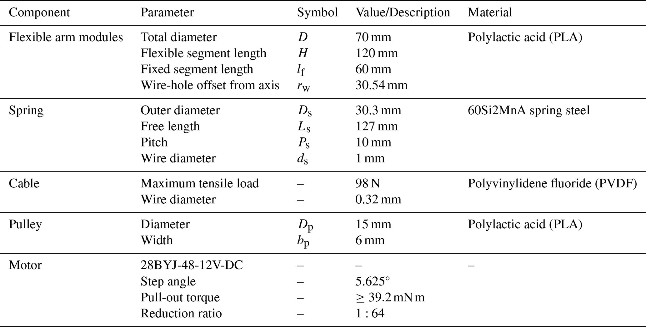
When operating in non-structured environments such as in narrow spaces for exploration and search and rescue operations, the soft snake-like robot not only needs to have excellent environmental adaptability but also needs to integrate the drive, perception and control systems to a high degree. Therefore, we designed a modular cable-driven soft snake-like robot, which is composed of five identical flexible arm modules connected in series, as shown in Fig. 1a. Each flexible arm module is an independent unit that integrates drive, perception and control, and it is composed of five core parts: flexible spine, drive system, perception system, support frame and control circuit. The micro-inertial sensors are installed at the end and midpoint positions along the central axis of the flexible arm module, as shown in Fig. 1b and c. The detailed design parameters of the flexible arm module are shown in Table 1.

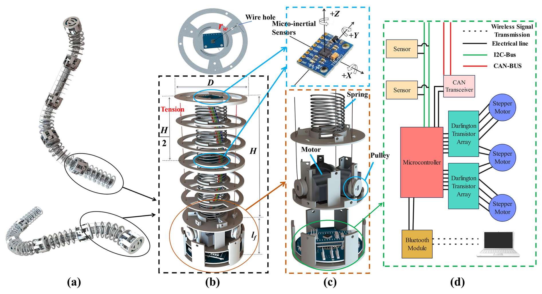
Figure 1 (a) The mechanical structure of the continuum snake-like robot. (b) The layout of micro-inertial sensors on the flexible arm module. (c) The drive system of the flexible arm module. (d) The control system schematic diagram of the snake-shaped robot.

To meet the real-time perception requirements of the soft snake-like robot, a distributed electronic control system based on CAN bus communication was designed. This system adopts a master–slave two-level control architecture. The master controller is responsible for motion planning, human–computer interaction and shape estimation after integrating data from each sub-unit. The sub-controllers within each flexible arm module independently complete the acquisition of bottom sensor data, attitude calculation and stepper motor control. Modules only exchange instructions and status information through the CAN bus. This architecture distributes computing tasks to each module, significantly reducing the computational burden of the main controller, while enhancing the scalability and fault tolerance of the system, as shown in Fig. 1d.

Table 1 Key parameters of hyper-redundant manipulator.

2.2 Serpentine gait driving equations

Each flexible arm module is independently actuated by three stepper motors, enabling arbitrary bending shapes through differential control of three cable displacements. To simplify the serpentine gait generation, we derive the following control equations:

$$\begin{array}{}\text{(1)}& \left\{\begin{array}{l}{L}_A={\displaystyle \frac{\mathrm{2}}{\mathrm{3}}}{L}_i\cos {\mathit{\sigma }}_i\\ L_B=-{\displaystyle \frac{\mathrm{2}}{\mathrm{3}}}{L}_i\sin \left({\mathit{\sigma }}_i+{\displaystyle \frac{\mathit{\pi }}{\mathrm{6}}}\right)\\ L_C={\displaystyle \frac{\mathrm{2}}{\mathrm{3}}}{L}_i\sin \left({\mathit{\sigma }}_i-{\displaystyle \frac{\mathit{\pi }}{\mathrm{6}}}\right).\end{array}\right..\end{array}$$

Here, L_A, L_B and L_C correspond to the displacements of each driving cable, while L_i and σ_i denote the variables illustrated in Fig. 2a, with $\mathit{\sigma }\in [\mathrm{0},\mathrm{2}\mathit{\pi }]$ and $i\in \mathit{\{}\mathrm{1},\mathrm{2},\mathrm{3},\mathrm{4},\mathrm{5}\mathit{\}}$. Taking undulatory locomotion as an example, the motion control process is depicted in Fig. 2b. In Sect. 4, we will experimentally validate the proposed real-time shape estimation method using gaits generated by this approach.

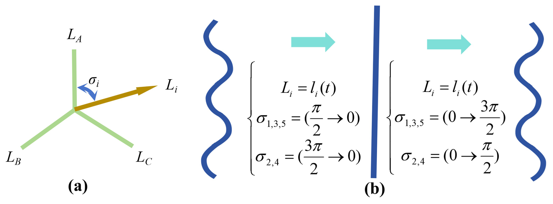
Figure 2 (a) The displacement vector L_i resulting from the synthesis of the cable's elongation and contraction. (b) The values of L_i and σ_i corresponding to the fluctuation curve.

3 Methodology

To achieve real-time shape prediction for the soft snake-like robot, it is first necessary to process the measurement data from the micro inertial sensors to obtain the rotation angles of the flexible arm modules. Based on the parabolic assumption theory, the bending shapes of each flexible arm module are then obtained. Subsequently, the complete morphological contour of the soft snake-like robot is synthesized through continuous coordinate transformation and curve splicing algorithms. The following is a detailed elaboration of the entire process of real-time shape prediction.

3.1 Processing of measurement data from micro-inertial sensors

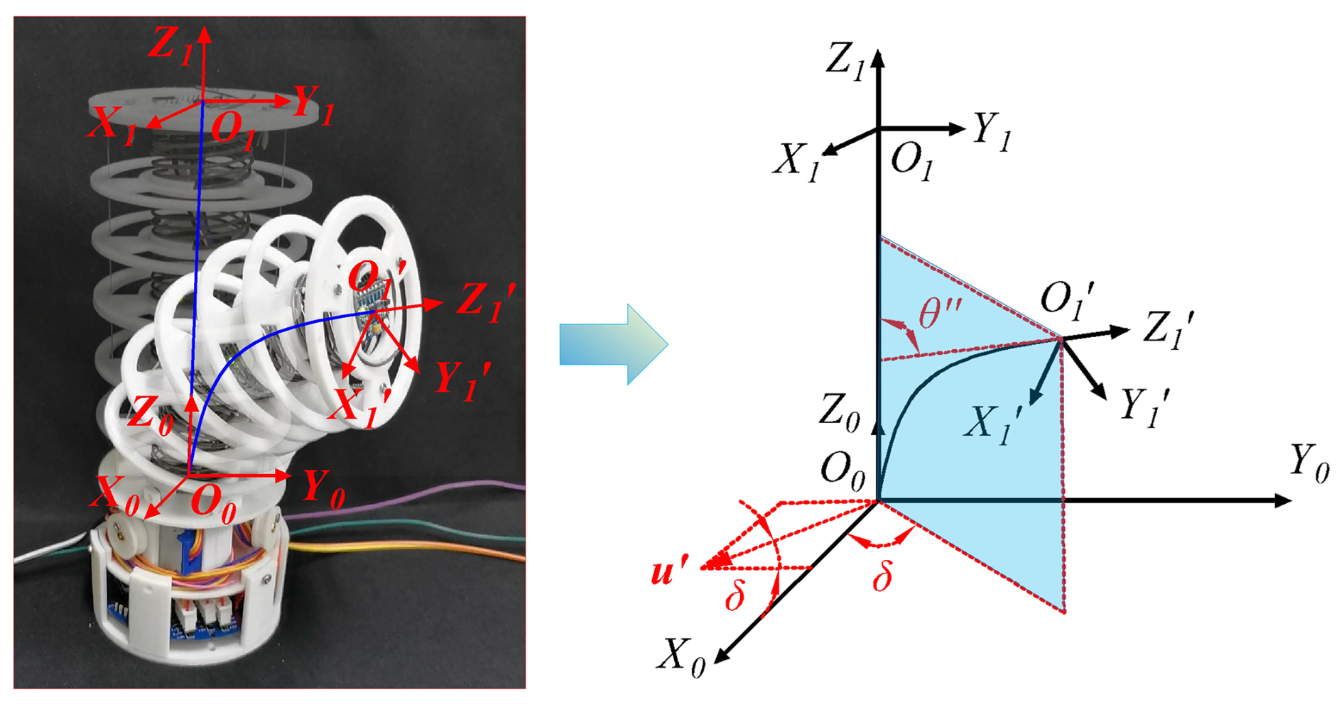
As shown in Fig. 3, six-axis attitude sensors are installed at the midpoint and the end point of the flexible arm module. These sensors incorporate a three-axis gyroscope and a three-axis accelerometer. The angular velocity at the measurement point is

$$\begin{array}{}\text{(2)}& {\mathit{\omega }}_{\mathrm{m}}=\mathit{\omega }+{\mathbf{b}}_{\mathit{\omega }}+{\mathit{\mu }}_{\mathit{\omega }},\end{array}$$

where ω_m denotes the measured angular velocity from the attitude sensor, ω represents the true angular velocity of the flexible arm, b_ω is the random measurement bias and μ_ω indicates Gaussian white noise.

Figure 3 The schematic diagram of the bending of the flexible arm.

The acceleration at the measurement point is

$$\begin{array}{}\text{(3)}& {\mathbf{a}}_{\mathrm{m}}={\mathbf{R}}_a(\mathbf{a}-{\left[\begin{array}{ccc}\mathrm{0}& \mathrm{0}& g\end{array}\right]}^{\mathrm{T}})+{\mathbf{b}}_a+{\mathit{\mu }}_a,\end{array}$$

where a_m is the measured acceleration from the attitude sensor, a represents the true acceleration in the inertial frame, R_a denotes the rotation matrix from rotary frame to inertial frame, g is gravitational acceleration and b_a and μ_a are the bias and noise terms, respectively.

To calculate the bending angle of the measurement points on the flexible arm, it is assumed that the flexible arm rotates successively around the coordinate axes, with the rotation sequence being $Z⟶Y⟶X$, and the rotation angles being θ_y, θ_p and θ_r, respectively. The following relationship holds:

$$\begin{array}{}\text{(4)}& \begin{array}{rl}& {\mathbf{R}}_a=\\ & \left[\begin{array}{ccc}c{\mathit{\theta }}_{\mathrm{p}}c{\mathit{\theta }}_y& c{\mathit{\theta }}_{\mathrm{p}}s{\mathit{\theta }}_y& -s{\mathit{\theta }}_{\mathrm{p}}\\ c{\mathit{\theta }}_{y}s{\mathit{\theta }}_{\mathrm{p}}s{\mathit{\theta }}_{\mathrm{r}}-c{\mathit{\theta }}_{\mathrm{r}}s{\mathit{\theta }}_y& c{\mathit{\theta }}_{\mathrm{r}}c{\mathit{\theta }}_y+s{\mathit{\theta }}_{\mathrm{p}}s{\mathit{\theta }}_{\mathrm{r}}s{\mathit{\theta }}_y& c{\mathit{\theta }}_{\mathrm{p}}s{\mathit{\theta }}_{\mathrm{r}}\\ s{\mathit{\theta }}_{\mathrm{r}}s{\mathit{\theta }}_y+c{\mathit{\theta }}_{\mathrm{r}}c{\mathit{\theta }}_{y}s{\mathit{\theta }}_{\mathrm{p}}& c{\mathit{\theta }}_{\mathrm{r}}s{\mathit{\theta }}_{\mathrm{p}}s{\mathit{\theta }}_y-c{\mathit{\theta }}_{y}s{\mathit{\theta }}_{\mathrm{r}}& c{\mathit{\theta }}_{\mathrm{p}}c{\mathit{\theta }}_{\mathrm{r}}\end{array}\right]\end{array},\end{array}$$

where c and s denote cos (⋅) and sin (⋅) operations, respectively.

Let Q and R be the covariance error matrices of process noise and measurement noise and ${\widehat{\mathbf{X}}}_k^{-}=\left[\begin{array}{ccc}{\mathit{\theta }}_y^{-}& {\mathit{\theta }}_{\mathrm{p}}^{-}& {\mathit{\theta }}_{\mathrm{r}}^{-}\end{array}\right]$ represent the predicted rotation angle matrix at the kth iteration. The prior equation of rotation angle matrix is as follows:

$$\begin{array}{}\text{(5)}& {\widehat{\mathbf{X}}}_k^{-}=\mathbf{A}{\widehat{\mathbf{X}}}_{k-\mathrm{1}}^{-}+\mathbf{B}\left({\mathbf{R}}_{\mathit{\omega }}{\mathit{\omega }}_{\mathrm{m}}\right),\end{array}$$

where

$$\begin{array}{rl}{\mathbf{R}}_{\mathit{\omega }}& =\left[\begin{array}{ccc}\mathrm{1}& s{\mathit{\theta }}_{\mathrm{p}}s{\mathit{\theta }}_{\mathrm{r}}/c{\mathit{\theta }}_{\mathrm{p}}& s{\mathit{\theta }}_{\mathrm{p}}c{\mathit{\theta }}_{\mathrm{r}}/c{\mathit{\theta }}_{\mathrm{p}}\\ \mathrm{0}& c{\mathit{\theta }}_{\mathrm{r}}& -s{\mathit{\theta }}_{\mathrm{r}}\\ \mathrm{0}& s{\mathit{\theta }}_{\mathrm{r}}/c{\mathit{\theta }}_{\mathrm{p}}& c{\mathit{\theta }}_{\mathrm{r}}/c{\mathit{\theta }}_{\mathrm{p}}\end{array}\right],\\ \mathbf{A}& ={\mathbf{I}}_{\mathrm{3}\times \mathrm{3}},\mathbf{B}=\mathrm{\Delta }t\cdot {\mathbf{I}}_{\mathrm{3}\times \mathrm{3}},\end{array}$$

and Δt represents the sampling time, which is set to 0.001 s.

Let the prior error covariance matrix be as follows:

$$\begin{array}{}\text{(6)}& {\mathbf{P}}_k^{-}={\mathbf{AP}}_{k-\mathrm{1}}{\mathbf{A}}^{\mathrm{T}}+\mathbf{Q},\end{array}$$

and the Kalman gain is as follows:

$$\begin{array}{}\text{(7)}& {\mathbf{K}}_k={\displaystyle \frac{{\mathbf{P}}_k^{-}{\mathbf{H}}^{\mathrm{T}}}{{\mathbf{HP}}_k^{-}{\mathbf{H}}^{\mathrm{T}}+\mathbf{R}}},\end{array}$$

where $\mathbf{H}={\mathbf{I}}_{\mathrm{3}\times \mathrm{3}}$.

Then the posterior estimation of the rotation angle matrix ${\widehat{\mathbf{X}}}_k=\left[\begin{array}{ccc}{\mathit{\theta }}_y& {\mathit{\theta }}_{\mathrm{p}}& {\mathit{\theta }}_{\mathrm{r}}\end{array}\right]$ is as follows:

$$\begin{array}{}\text{(8)}& {\widehat{\mathbf{X}}}_k={\widehat{\mathbf{X}}}_k^{-}+{\mathbf{K}}_k({\mathbf{Z}}_k-\mathbf{H}{\widehat{\mathbf{X}}}_k^{-}),\end{array}$$

where ${\mathbf{Z}}_k=\mathbf{H}{\left[\begin{array}{ccc}\arctan \frac{a_y}{a_z}& -\arctan \frac{a_x}{\sqrt{a_y^{\mathrm{2}}+a_z^{\mathrm{2}}}}& \mathrm{0}\end{array}\right]}^{\mathrm{T}}$.

Finally, the updated covariance matrix is expressed as

$$\begin{array}{}\text{(9)}& {\mathbf{P}}_k=(\mathbf{I}-{\mathbf{K}}_k\mathbf{H}){\mathbf{P}}_k^{-}.\end{array}$$

Through experimental validation, the parameters and initial values involved in the aforementioned equations are determined as ${\mathbf{X}}_{\mathrm{0}}=\mathrm{0}\times {\mathbf{I}}_{\mathrm{3}\times \mathrm{3}}$, ${\mathbf{P}}_{\mathrm{0}}={\mathbf{I}}_{\mathrm{3}\times \mathrm{3}}$, $\mathbf{Q}=\mathrm{0.0025}\times {\mathbf{I}}_{\mathrm{3}\times \mathrm{3}}$, $\mathbf{R}=\mathrm{0.3}\times {\mathbf{I}}_{\mathrm{3}\times \mathrm{3}}$.

3.2 Parabolic assumption and pose estimation

The piecewise constant-curvature model (PCC) has been widely applied in the design, perception and control of continuum robots due to its simple modeling and convenient calculation. However, the PCC model still has some serious drawbacks. Due to factors such as friction and gravity, deviations exist between actual continuum robots and the overly simplified model (Cheng et al., 2022). Della Santina and Rus (2020) introduced a polynomial curvature model in control research, effectively solving the modeling problem of non-constant-curvature distribution. This suggests extending the polynomial-curvature approach to a simpler parabolic (quadratic) curvature assumption under restricted deformation conditions. It is worth noting that the parabolic assumption does not hold in all cases. Its application requires the following strict conditions: (1) the flexible arm undergoes small curvature or small bending angle deformation, where the slope of its centerline is much less than 1 ($y^{\prime }\ll \mathrm{1}$). (2) During bending of the flexible arm, the arc length of its centerline remains unchanged (i.e., inextensible), and the effect of lateral shear forces on deformation is ignored. In this paper, the flexible arm is actuated by tension from three uniformly arranged internal steel cables, and no lateral concentrated forces or distributed loads are applied. Moreover, the flexible arm consists of a uniform helical tension spring, and its equivalent flexural stiffness EI_eq can be regarded as constant along its length. Therefore, this flexible arm can be equivalently treated as an Euler–Bernoulli beam with uniform cross-section, and its flexural stiffness dominates the deformation. The initial undeformed central axis of the flexible arm is taken as the x axis, the deflection as y(x) and the bending moment along the centerline as M(x). The precise differential equation for the flexure curve of the flexible arm is as follows:

$$\begin{array}{}\text{(10)}& {\displaystyle \frac{y^{\prime \prime }}{(\mathrm{1}+(y^{\prime }{)}^{\mathrm{2}}{)}^{\mathrm{3}/\mathrm{2}}}}={\displaystyle \frac{M\left(x\right)}{{\text{EI}}_{\text{eq}}}}.\end{array}$$

Under the assumption of small curvature, the slope y^′ of the deformed flexible arm satisfies $y^{\prime }\ll \mathrm{1}$, so $(\mathrm{1}+(y^{\prime }{)}^{\mathrm{2}}{)}^{\mathrm{3}/\mathrm{2}}\approx \mathrm{1}$, and Eq. (10) can be simplified as

$$\begin{array}{}\text{(11)}& y^{\prime \prime }={\displaystyle \frac{M\left(x\right)}{{\text{EI}}_{\text{eq}}}}.\end{array}$$

Because the three uniformly arranged steel cables produce a transversely symmetric action at the free end, no net transverse shear is developed along the arm, consequently the internal bending moment is nearly constant, M(x)≈M₀, integrating Eq. (11) gives

$$\begin{array}{}\text{(12)}& y\left(x\right)={\displaystyle \frac{M_{\mathrm{0}}}{\mathrm{2}{\text{EI}}_{\text{eq}}}}{x}^{\mathrm{2}}+bx+c=a{x}^{\mathrm{2}}+bx+c.\end{array}$$

While Eq. (11) replaces the exact curvature $k_{\mathrm{e}}=M\left(x\right)/{\text{EI}}_{\text{eq}}$ in Eq. (10) with the small-deflection approximation $k_a=y^{\prime \prime }$, the resulting error is purely geometric and depends only on the local slope angle $\mathit{\varphi }=\arctan y^{\prime }$:

$$\begin{array}{}\text{(13)}& E_k=\left|{\displaystyle \frac{k_a-k_{\mathrm{e}}}{k_{\mathrm{e}}}}\right|=se{c}^{\mathrm{3}}\mathit{\varphi }-\mathrm{1}.\end{array}$$

Since E_k increases monotonically with the slope, imposing a tolerance $E_k\le E_k^{*}$ yields the admissible end tangent angle and the corresponding curvature upper bound:

$$\begin{array}{}\text{(14)}& {\displaystyle }{\mathit{\varphi }}_{max}& {\displaystyle }=\arccos \left({\displaystyle \frac{\mathrm{1}}{\sqrt[\mathrm{3}]{\mathrm{1}+E_k^{*}}}}\right),\text{(15)}& {\displaystyle }{k}_{max}& {\displaystyle }={\displaystyle \frac{\tan {\mathit{\varphi }}_{max}}{H}},\end{array}$$

where H is the length of the flexible arm.

With $E_k^{*}=\mathrm{5}$ %, Eqs. (14) and (15) give ${\mathit{\varphi }}_{max}=\mathrm{10.31}\mathit{°},k_{max}$. For the flexible arm length H=114.5 mm, the admissible curvature is therefore $k_{max}\approx \mathrm{1.59}{\mathrm{m}}^{-\mathrm{1}}$.

To confirm that the parabolic solution satisfies the beam equilibrium within the admissible range, we define the equilibrium residual as the maximum normalized imbalance between the bending moment implied by the assumed curvature and the actual bending moment:

$$\begin{array}{}\text{(16)}& E_M={\displaystyle \frac{max\left|{\text{EI}}_{\text{eq}}{k}_a\right(x)-M(x\left)\right|}{M_{\mathrm{0}}}}.\end{array}$$

Because the actuating moment is nearly constant along the arm, M(x)≈M₀, substituting the parabolic deflection Eq. (12) into the equilibrium Eq. (11) yields ${\text{EI}}_{\text{eq}}{k}_a=M_{\mathrm{0}}=M\left(x\right)$ for all x, hence E_M=0. The admissible curvature range $k\le k_{max}$ therefore satisfies the moment balance as well, so the geometric bound $E_k\le E_k^{*}$ and the mechanical equilibrium condition are met simultaneously.

If a parabola passes through the origin (0,0) and the point (m,0), the tangent line of the parabola forms an angle φ with the positive direction of the X axis, as shown in Fig. 4a and b. Assuming the parabolic equation is $y=a{x}^{\mathrm{2}}+bx$, then

$$\begin{array}{}\text{(17)}& {\displaystyle }& {\displaystyle }\mathrm{0}=a{m}^{\mathrm{2}}+bm,\text{(18)}& {\displaystyle }& {\displaystyle }\tan \mathit{\varphi }=-b,\text{(19)}& {\displaystyle }& {\displaystyle }S=\underset{\mathrm{0}}{\overset{m}{\int }}\sqrt{\mathrm{1}+(\mathrm{2}ax+b{)}^{\mathrm{2}}}\mathrm{d}x,\end{array}$$

where the parabolic arc length S is defined as the arithmetic mean of the internal cable lengths: $S=(L_{\mathrm{1}}+L_{\mathrm{2}}+L_{\mathrm{3}})/\mathrm{3}$, with L₁, L₂ and L₃ denoting the lengths of the three cables inside the flexible arm.

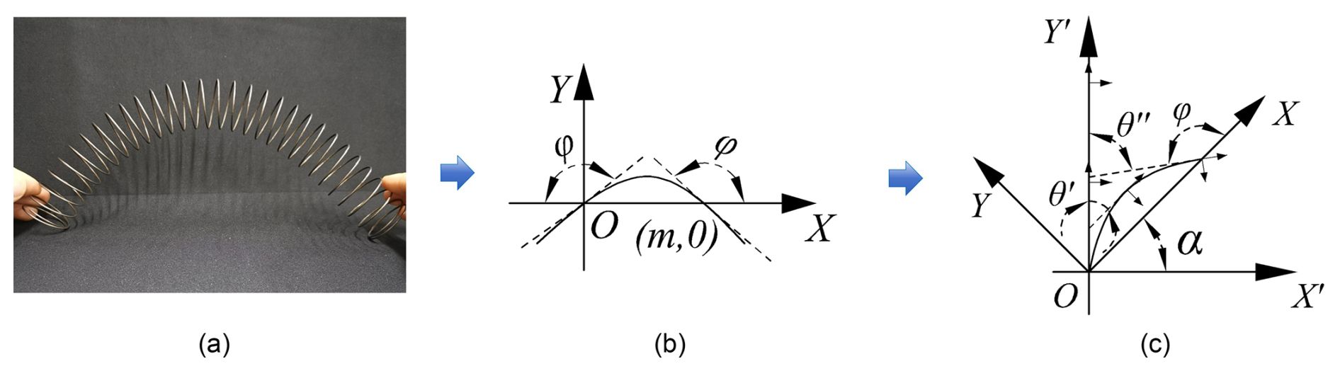
Figure 4 (a) The bent spring configuration approximates a parabolic profile. (b) Simplified as a parabola passing through the coordinate origin. (c) The XY coordinate system rotated counterclockwise by angle α about the origin.

As shown in Fig. 4c, when the XY coordinate system is rotated counterclockwise by an angle α about the origin O, the following relationship can be derived based on geometric constraints:

$$\begin{array}{}\text{(20)}& {\displaystyle }\mathit{\varphi }& {\displaystyle }=\mathit{\pi }-{\mathit{\theta }}^{\prime \prime }+{\mathit{\theta }}^{\prime },\text{(21)}& {\displaystyle }\mathit{\alpha }& {\displaystyle }=\mathit{\pi }/\mathrm{2}-{\mathit{\theta }}^{\prime },\end{array}$$

where θ^′ represents the angle formed by the tangent line at the midpoint of the flexible arm module and the y axis, while θ^′′ represents the angle formed by the tangent line at the end point of the flexible arm module and the y axis. Angles θ^′ and θ^′′ are obtained by fusing the rotation angle data at key points of the flexible arm module, and the calculation formula is as follows:

$$\begin{array}{}\text{(22)}& \left\{\begin{array}{l}{\mathit{\theta }}^{\prime }=\sqrt{{{\mathit{\theta }}_{\mathrm{p}}^{\prime }}^{\mathrm{2}}+{{\mathit{\theta }}_{\mathrm{r}}^{\prime }}^{\mathrm{2}}}\\ {\mathit{\theta }}^{\prime \prime }=\sqrt{{{\mathit{\theta }}_{\mathrm{p}}^{\prime \prime }}^{\mathrm{2}}+{{\mathit{\theta }}_{\mathrm{r}}^{\prime \prime }}^{\mathrm{2}}}\end{array}\right.,\end{array}$$

where ${\mathit{\theta }}_{\mathrm{p}}^{\prime }$ and ${\mathit{\theta }}_{\mathrm{r}}^{\prime }$ represent the rotation angles of the midpoint position of the flexible arm module around the Y axis and X axis, respectively, ${\mathit{\theta }}_{\mathrm{p}}^{\prime \prime }$ and ${\mathit{\theta }}_{\mathrm{r}}^{\prime \prime }$ represent the rotation angles of the endpoint position of the flexible arm module around the Y axis and X axis, respectively. The values of angles were obtained through the method described in Sect. 3.1.

The unknown parameters a, b, m, φ and α are determined by solving the system of Eqs. (17)–(21).

Furthermore, it is necessary to solve the homogeneous coordinate transformation matrix between two adjacent flexible arm modules in order to predict the overall shape of a soft robot. Set the base point coordinate system of the (i−1)th flexible arm module as $\mathit{\left\{}{O}_{i-\mathrm{1}}{X}_{i-\mathrm{1}}{Y}_{i-\mathrm{1}}{Z}_{i-\mathrm{1}}\mathit{\right\}}$ and that of the ith flexible arm module as {O_iX_iY_iZ_i}. Suppose that the unit vector of a certain axis passing through the origin O_i−1 of the coordinate system $\mathit{\left\{}{O}_{i-\mathrm{1}}{X}_{i-\mathrm{1}}{Y}_{i-\mathrm{1}}{Z}_{i-\mathrm{1}}\mathit{\right\}}$ is ${\mathbf{u}}^{\prime }=(u_x,u_y,u_z)=(\sin \mathit{\delta },\cos \mathit{\delta },\mathrm{0})$ and the (i−1)th flexible arm module rotates by α around a certain axis u^′. It should be noted that the setting of u_z=0 here is because the snake-like robot in this study design lacks the rotational degree of freedom around the Z axis. However, the method presented in this article is also applicable to the case of rotating around any axis. Then the angle between the bending section of the (i−1)th flexible arm module and the X_i−1 axis is $\mathit{\delta }=\arctan \left(\right({\mathit{\theta }}_{\mathrm{r}}^{\prime }+{\mathit{\theta }}_{\mathrm{r}}^{\prime \prime })/({\mathit{\theta }}_{\mathrm{p}}^{\prime }+{\mathit{\theta }}_{\mathrm{p}}^{\prime \prime }\left)\right)$, and the coordinates of the origin O_i of the coordinate system {O_iX_iY_iZ_i} can be obtained as $O_i=(m\cos \mathit{\alpha }\cos \mathit{\delta },m\cos \mathit{\alpha }\sin \mathit{\delta },m\sin \mathit{\alpha })$. Thus, the homogeneous transformation matrix ${}_i^{i-\mathrm{1}}\mathbf{T}$ between the flexible arm module i−1 and the flexible arm module i can be obtained as

$$\begin{array}{}\text{(23)}& \begin{array}{rl}& {}_i^{i-\mathrm{1}}\mathbf{T}=\\ & \left[\begin{array}{cccc}\mathrm{1}-\mathrm{2}{q}_{\mathrm{2}}^{\mathrm{2}}& \mathrm{2}{q}_{\mathrm{1}}{q}_{\mathrm{2}}& \mathrm{2}{q}_{\mathrm{0}}{q}_{\mathrm{2}}& mc\mathit{\alpha }c\mathit{\delta }\\ \mathrm{2}{q}_{\mathrm{1}}{q}_{\mathrm{2}}& \mathrm{1}-\mathrm{2}{q}_{\mathrm{1}}^{\mathrm{2}}& -\mathrm{2}{q}_{\mathrm{0}}{q}_{\mathrm{1}}& mc\mathit{\alpha }s\mathit{\delta }\\ -\mathrm{2}{q}_{\mathrm{0}}{q}_{\mathrm{2}}& \mathrm{2}{q}_{\mathrm{0}}{q}_{\mathrm{1}}& \mathrm{1}-\mathrm{2}{q}_{\mathrm{1}}^{\mathrm{2}}-\mathrm{2}{q}_{\mathrm{2}}^{\mathrm{2}}& ms\mathit{\alpha }\\ \mathrm{0}& \mathrm{0}& \mathrm{0}& \mathrm{1}\end{array}\right]\end{array},\end{array}$$

where $q_{\mathrm{0}}=\cos ({\mathit{\theta }}^{\prime \prime }/\mathrm{2})$, $q_{\mathrm{1}}=u_x\cdot \sin ({\mathit{\theta }}^{\prime \prime }/\mathrm{2})$, $q_{\mathrm{2}}=u_y\cdot \sin ({\mathit{\theta }}^{\prime \prime }/\mathrm{2})$, q₃=0.

3.3 Error compensation strategy

In actual engineering, numerous factors, such as the manufacturing process of the spring, the assembly accuracy of the flexible arm module and the uneven distribution of force, can lead to the spring's bent shape not being a perfectly symmetrical parabolic shape. To accurately predict the bending shape of the flexible arm module, a shape compensation strategy based on sensor position offset is proposed.

When the shape of the spring's bending is completely symmetrical parabolic, the maximum amplitude of the parabola is at the midpoint of the spring. The tangent line passing through the midpoint of the spring is parallel to the line connecting the beginning and end points of the spring. If the maximum amplitude of the parabola shifts towards the end of the spring, the angle between the tangent line at the midpoint and the line connecting the beginning and end points of the spring is an acute angle, as shown in Fig. 5a. According to the geometric relationship in Fig. 5b, if the micro-inertial sensor is installed at the midpoint of the spring, the angle of deflection measured by the sensor is lower than the actual value. If the maximum amplitude of the parabola shifts towards the beginning of the spring, the angle between the tangent line at the midpoint and the line connecting the beginning and end points of the spring is an obtuse angle, as shown in Fig. 5c. According to the geometric relationship in Fig. 5d, if the micro-inertial sensor is installed at the midpoint of the spring, the angle of deflection measured by the sensor is higher than the actual value. Therefore, the position of the sensor installed at the midpoint of the spring needs to be adjusted according to the actual situation to reduce the error between the measured value and the actual value.

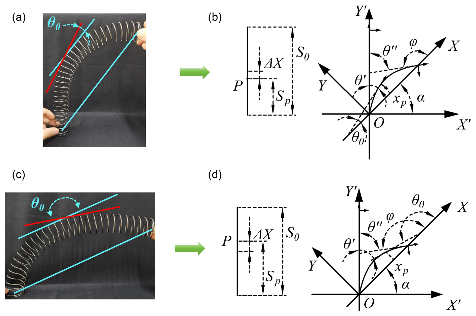
Figure 5 (a) The midpoint deflection angle measured by the sensor underestimates the true value. (b) Underestimation correction. (c) The sensor-measured deflection angle overestimates the true value. (d) Overestimation correction.

Suppose the sensor installed at the midpoint of the spring is shifted by ΔX (in the case of Fig. 5a, it is shifted towards the spring's starting point by ΔX, and the value is negative. In the case of Fig. 5c, it is shifted towards the spring's end point by ΔX, and the value is positive). Let the original length of the spring be S₀ and P point be the installation position of the sensor. Then, the rope in the flexible arm module contracts, causing the spring to bend. After bending, the length of the spring is S₁, and the compression rate of the spring is $\mathit{\lambda }=S_{\mathrm{1}}/S_{\mathrm{0}}$. After the spring contracts, the arc length from point O (the base point) to point P is $S_{p^{\prime }}=\mathit{\lambda }{S}_{\mathrm{p}}$. Referring to the previous section, the following equations can be derived:

$$\begin{array}{}\text{(24)}& {\displaystyle }& {\displaystyle }{S}_{\mathrm{1}}=\underset{\mathrm{0}}{\overset{m}{\int }}\sqrt{\mathrm{1}+(\mathrm{2}ax+b{)}^{\mathrm{2}}}\mathrm{d}x,\text{(25)}& {\displaystyle }& {\displaystyle }{S}_{p^{\prime }}=\underset{\mathrm{0}}{\overset{x_{\mathrm{p}}}{\int }}\sqrt{\mathrm{1}+(\mathrm{2}ax+b{)}^{\mathrm{2}}}\mathrm{d}x,\text{(26)}& {\displaystyle }& {\displaystyle }\tan {\mathit{\theta }}_{\mathrm{0}}=\mathrm{2}a{x}_{\mathrm{p}}+b,\text{(27)}& {\displaystyle }& {\displaystyle }{\mathit{\theta }}_{\mathrm{0}}+{\mathit{\theta }}^{\prime }+\mathit{\pi }-{\mathit{\theta }}^{\prime \prime }=\mathit{\varphi },\text{(28)}& {\displaystyle }& {\displaystyle }\mathit{\alpha }=\mathit{\pi }/\mathrm{2}-{\mathit{\theta }}_{\mathrm{0}}-{\mathit{\theta }}^{\prime },\end{array}$$

where θ₀ is the angle between the tangent at point P and the X axis. By solving Eqs. (24)–(28) simultaneously, numerical solutions for a, b, m, φ, x_p, θ₀ and α can be obtained. Since ΔX is primarily an estimation parameter dependent on the spring's axial deformation, it can be empirically calibrated based on experimental data. We define its quantitative relationship as follows:

$$\begin{array}{}\text{(29)}& \mathrm{\Delta }X=\mathrm{\Delta }{x}_{\mathrm{0}}+\mathit{\kappa }\ln (S_{\mathrm{0}}-S_t),\end{array}$$

where Δx₀ represents the deviation between the sensor and the central axis of the flexible backbone in the actual assembly, which can be measured post-assembly. S₀ denotes the initial length of the HRM, and S_t is its real-time length. κ is an undetermined coefficient to be calibrated experimentally.

To reduce the dependence on purely empirical tuning, Δx₀ is treated as a fixed geometric parameter measured once by laser ranging after assembly, and the scalar coefficient κ is determined by a two-stage procedure: an offline batch baseline with a batch-derived correction, followed by a lightweight online drift-adaptive fine-tuning.

Figure 6 Batch calibration accuracy.

(1) Offline batch baseline

Calibration tests were conducted on n representative specimens of the same material and structure design (the specific process is described in Sect. 4.2). For each specimen i, Δx_0,i represents the deviation between the sensor and the center point of the flexible spine, the coefficient κ_0,i was determined using the least squares regression method to minimize the root-mean-square error (RMSE) between the predicted value and the actual value, thereby obtaining the batch baseline and its dispersion.

$$\begin{array}{}\text{(30)}& {\stackrel{\mathrm{‾}}{\mathit{\kappa }}}_{\mathrm{0}}={\displaystyle \frac{\mathrm{1}}{n}}\sum _{i=\mathrm{1}}^n{\mathit{\kappa }}_{\mathrm{0},i},{\mathit{\sigma }}_{\mathit{\kappa }}=\sqrt{{\displaystyle \frac{\mathrm{1}}{n-\mathrm{1}}}\sum _{i=\mathrm{1}}^n({\mathit{\kappa }}_{\mathrm{0},i}-{\stackrel{\mathrm{‾}}{\mathit{\kappa }}}_{\mathrm{0}}{)}^{\mathrm{2}}}\end{array}$$

Because machining and assembly tolerances couple κ with the measurable assembly offset, a linear correction is estimated over the n specimens:

$$\begin{array}{}\text{(31)}& {\displaystyle }& {\displaystyle }{k}_i={\stackrel{\mathrm{‾}}{k}}_{\mathrm{0}}+C(\mathrm{\Delta }{x}_{\mathrm{0},i}-\mathrm{\Delta }{\stackrel{\mathrm{‾}}{x}}_{\mathrm{0}}),\mathrm{\Delta }{\stackrel{\mathrm{‾}}{x}}_{\mathrm{0}}={\displaystyle \frac{\mathrm{1}}{n}}\sum _{i=\mathrm{1}}^n\mathrm{\Delta }{x}_{\mathrm{0},i},\text{(32)}& {\displaystyle }& {\displaystyle }C={\displaystyle \frac{{\sum }_{i=\mathrm{1}}^n(\mathrm{\Delta }{x}_{\mathrm{0},i}-\mathrm{\Delta }{\stackrel{\mathrm{‾}}{x}}_{\mathrm{0}})({\mathit{\kappa }}_i-{\stackrel{\mathrm{‾}}{\mathit{\kappa }}}_{\mathrm{0}})}{{\sum }_{i=\mathrm{1}}^n(\mathrm{\Delta }{x}_{\mathrm{0},i}-\mathrm{\Delta }{\stackrel{\mathrm{‾}}{x}}_{\mathrm{0}}{)}^{\mathrm{2}}}}.\end{array}$$

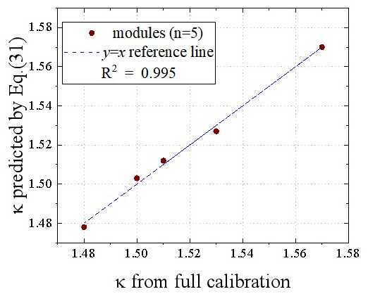
Because machining and assembly tolerances couple κ with the measurable assembly offset, a linear correction is estimated over a homogeneous batch of modules with identical outer diameter (30.54 mm) and height (114.5 mm). For five modules with $\mathrm{\Delta }{x}_{\mathrm{0}}=\mathit{\{}\mathrm{1.75},\mathrm{1.63},\mathrm{1.82},\mathrm{1.77},\mathrm{1.72}\mathit{\}}\mathrm{mm}$ and $\mathit{\kappa }=\mathit{\{}\mathrm{1.51},\mathrm{1.57},\mathrm{1.48},\mathrm{1.50},\mathrm{1.53}\mathit{\}}$, the baseline is ${\stackrel{\mathrm{‾}}{\mathit{\kappa }}}_{\mathrm{0}}=\mathrm{1.518}$ with σ_κ=0.034 and $\mathrm{\Delta }{\stackrel{\mathrm{‾}}{x}}_{\mathrm{0}}=\mathrm{1.738}\mathrm{mm}$. The least-squares regression gives $C=-\mathrm{0.484}$, with a coefficient of determination R²≈0.995. Since R²≥0.8, the correction is retained, so any other module j of the same batch obtains its coefficient from the laser-measured offset alone, ${\mathit{\kappa }}_j={\stackrel{\mathrm{‾}}{\mathit{\kappa }}}_{\mathrm{0}}+C(\mathrm{\Delta }{x}_{\mathrm{0},j}-\mathrm{\Delta }{\stackrel{\mathrm{‾}}{x}}_{\mathrm{0}})$, thereby eliminating repeated full calibration. The admissible range is $[{\mathit{\kappa }}_{\text{min}},{\mathit{\kappa }}_{max}]={\stackrel{\mathrm{‾}}{\mathit{\kappa }}}_{\mathrm{0}}\pm \mathrm{3}{\mathit{\sigma }}_{\mathit{\kappa }}=[\mathrm{1.415},\mathrm{1.621}]$. Figure 6 compares the predicted coefficients with those from full calibration; the mean and maximum relative prediction errors are 0.13 % and 0.22 %, respectively.

Figure 7 Online drift-adaptive compensation.

(2) Online drift-adaptive update

During long-duration motion, spring creep and joint abrasion induce slow drift of κ. Here, it is assumed that the micro-inertial sensor installed on the end face of the flexible arm coincides with the center point of the end face. The deflection angle θ^′′ measured by the sensor is the actual deflection angle, and no online error compensation is performed. Let ${\mathit{\theta }}_k^{\prime }$

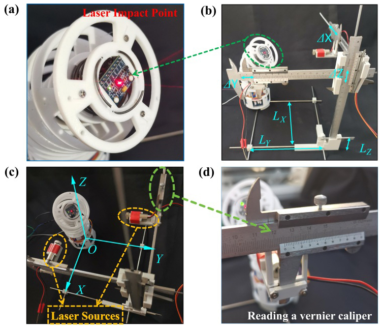
Figure 8 (a) Laser spot aligned with the sensor's central position. (b) Measurement of relative coordinate values generated by the flexible arms' motion. (c) Laser generators fixed on the X and Y axis verniers. (d) Scale readings with 0.02 mm precision.

represent the deflection angle acquired by the sensor installed at the middle position of the flexible arm at the kth sampling period. For all subsequent variables, the subscript k stands for the variable value at time k. With the middle offset $\mathrm{\Delta }{X}_k=\mathrm{\Delta }{x}_{\mathrm{0}}+{\mathit{\kappa }}_k\ln (S_{\mathrm{0}}-S_{tk})$, the predicted deflection angle ${\mathit{\theta }}^{{\widehat{\prime }}_k}$ is

$$\begin{array}{}\text{(33)}& {\widehat{\mathit{\theta }}}_k^{\prime }=f(\mathrm{\Delta }{x}_{\mathrm{0}}+{\mathit{\kappa }}_k\ln (S_{\mathrm{0}}-S_{tk}\left)\right),\end{array}$$

where f(⋅) denotes the forward solution of Eqs. (24)–(28). For the top position, the tangent-angle constraint $\tan {\mathit{\theta }}^{\prime \prime }=\mathrm{2}a\cdot x\left(m\right)+b$, together with the middle constraint $\tan {\widehat{\mathit{\theta }}}_k^{\prime }=\mathrm{2}a\cdot x(S_{\mathrm{0}}/\mathrm{2}+\mathrm{\Delta }{X}_k)+b$; the parabola $y=a{x}^{\mathrm{2}}+bx$ is uniquely determined and the middle angle ${\widehat{\mathit{\theta }}}_k^{\prime }$ follows.

The sensitivity of the predicted angle ${\widehat{\mathit{\theta }}}_k^{\prime }$ with respect to the scalar κ_k is evaluated numerically by a central finite difference on the solved geometry,

$$\begin{array}{}\text{(34)}& \begin{array}{rl}{J}_k& ={\displaystyle \frac{\partial {\widehat{\mathit{\theta }}}_k^{\prime }}{\partial {\mathit{\kappa }}_k}}={\displaystyle \frac{\begin{array}{l}f(\mathrm{\Delta }{x}_{\mathrm{0}}+({\mathit{\kappa }}_k+\mathit{\delta }\left)\ln \right(S_{\mathrm{0}}-S_{tk}\left)\right)\end{array}}{\mathrm{2}\mathit{\delta }}}-\\ & {\displaystyle \frac{\begin{array}{l}f(\mathrm{\Delta }{x}_{\mathrm{0}}+({\mathit{\kappa }}_k-\mathit{\delta }\left)\ln \right(S_{\mathrm{0}}-S_{tk}\left)\right)\end{array}}{\mathrm{2}\mathit{\delta }}},\end{array}\end{array}$$

with step $\mathit{\delta }=\mathrm{1}\times {\mathrm{10}}^{-\mathrm{4}}$, and the scalar coefficient is fine-tuned within the band $[{\mathit{\kappa }}_{\text{min}},{\mathit{\kappa }}_{max}]$ by the normalized least-mean-square update driven by the scalar middle-angle error:

$$\begin{array}{}\text{(35)}& \begin{array}{rl}& {\mathit{\kappa }}_{k+\mathrm{1}}={\mathit{\kappa }}_k+{\mathit{\eta }}_k{J}_k{e}_k,{\mathit{\eta }}_k=\mathit{\mu }/\left(\mathit{ϵ}+J_k^{\mathrm{2}}\right),\\ & {\mathit{\kappa }}_{k+\mathrm{1}}=\text{proj}[{\mathit{\kappa }}_{\text{min}},{\mathit{\kappa }}_{max}]\left({\mathit{\kappa }}_{k+\mathrm{1}}\right),e_k={\mathit{\theta }}_k^{\prime }-{\widehat{\mathit{\theta }}}_k^{\prime }\end{array},\end{array}$$

where $\mathrm{0}<\mathit{\mu }<\mathrm{2}$, $\mathit{ϵ}=max(\mathrm{1}\times {\mathrm{10}}^{-\mathrm{6}},|{\mathit{\kappa }}_k|\times {\mathrm{10}}^{-\mathrm{4}})$.

Figure 9 Sample of the flexible arm.

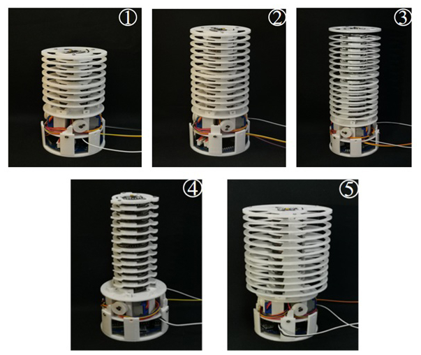
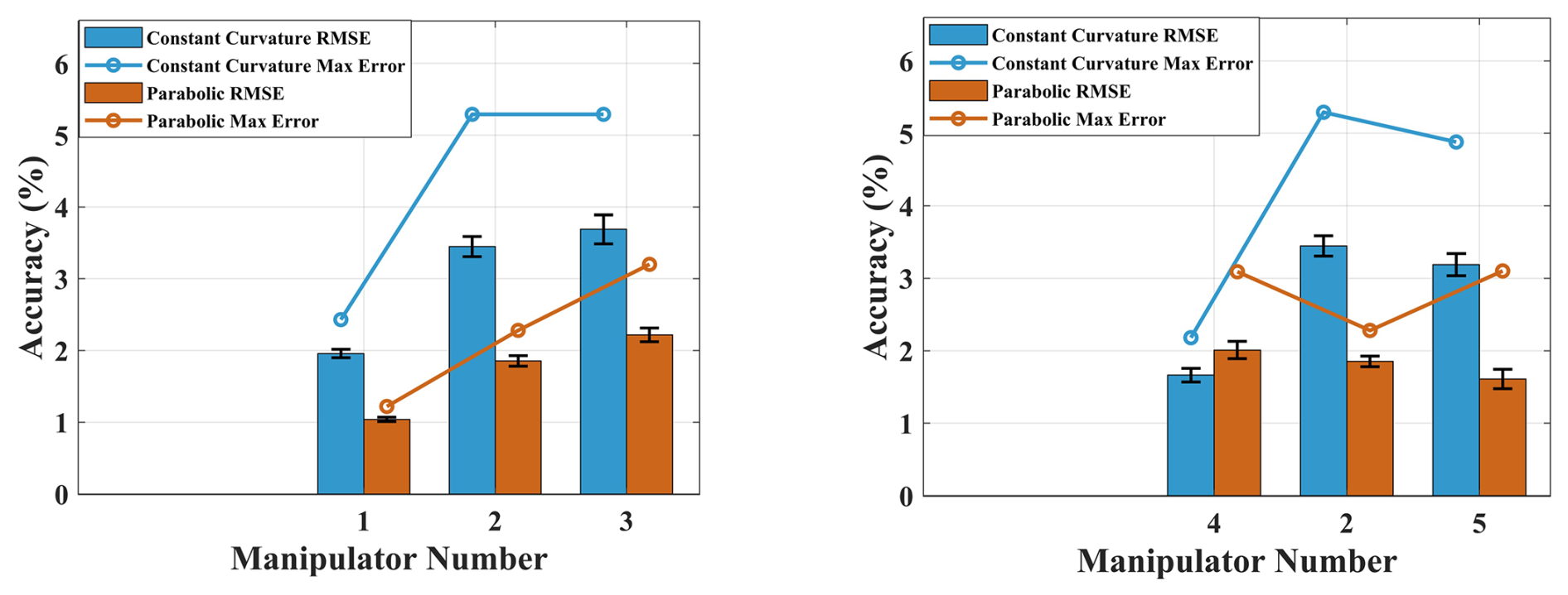
Figure 10 Comparison of positioning errors of the flexible arms in constant-curvature model and parabolic model.

Table 2 Calibration results of flexible arm.

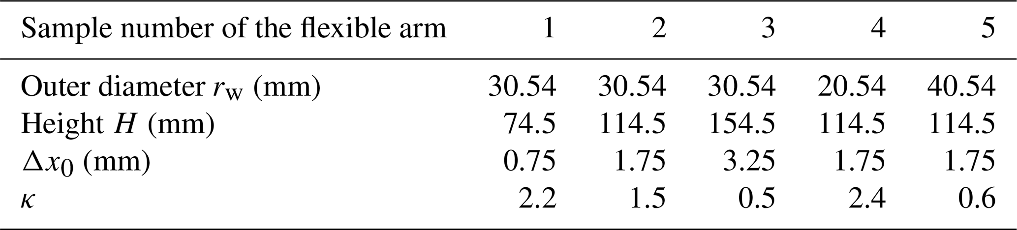
Table 3 Dynamic real-time performance metrics of shape estimation.

(3) Convergence and stopping criterion

Under $\mathrm{0}<\mathit{\mu }<\mathrm{2}$ the update is stable; when ln (S₀−S_tk) persistently excites the two geometric constraints over the operating range (so that ${\sum }_k{J}_k^{\mathrm{2}}>\mathrm{0}$), κ_k converges to the drift-free value and e_k→0. The projection in Eq. (35) keeps κ_k bounded, so the residual error remains bounded by the slow drift. The scalar residual is constructed from the middle inertial sensor, while the fixed top reference is only used to solve the forward geometric model. External measurement equipment such as a laser tracker is adopted offline to establish the absolute baseline and calibrate the standard deviation σ_s of sensor noise. The root-mean-square residual of the sliding window at the kth moment is calculated by the following formula:

$$\begin{array}{}\text{(36)}& R_k=\sqrt{{\displaystyle \frac{\mathrm{1}}{W}}\sum _{i=k-W+\mathrm{1}}^k{e}_i^{\mathrm{2}}}.\end{array}$$

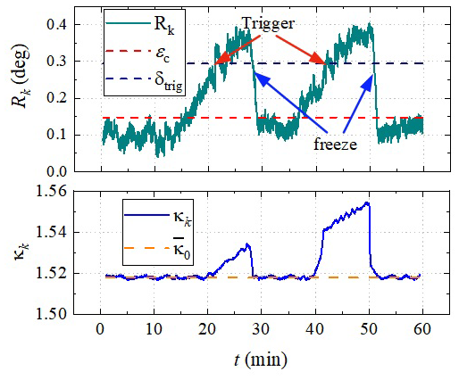
To avoid unnecessary iterative updates of parameters, the adaptation mechanism is activated only when the sliding-window residual R_k exceeds the preset threshold δ_trig=3σ_s and freezes when R_k stays below the convergence threshold ϵ_c=1.5σ_s for N consecutive windows.

The sliding-window residual R_k and the online coefficient κ_k over this period are shown in Fig. 7. With a window length W=100 and a static angle-noise level σ_s=0.098°, the activation and convergence thresholds were set to ${\mathit{\delta }}_{\text{trig}}=\mathrm{3}{\mathit{\sigma }}_{\mathrm{s}}=\mathrm{0.294}\mathit{°}$ and ${\mathit{ϵ}}_{\mathrm{c}}=\mathrm{1.5}{\mathit{\sigma }}_{\mathrm{s}}=\mathrm{0.147}\mathit{°}$. As the residual rose above δ_trig near the 20th and 45th minutes (adaptation triggered), the coefficient κ_k was adjusted within a narrow band around the batch baseline ${\stackrel{\mathrm{‾}}{\mathit{\kappa }}}_{\mathrm{0}}=\mathrm{1.518}$; the residual was then pulled back below ϵ_c, and the adaptation froze once it stayed there for several consecutive windows. The two complete trigger–convergence–freeze cycles show that the online update compensates for the slow parameter drift caused by spring fatigue and cable relaxation, keeping the estimation error within the acceptable band over the whole run. The coefficient never reached the admissible limits $[{\mathit{\kappa }}_{\text{min}},{\mathit{\kappa }}_{max}]$, confirming that the offline batch calibration already provides a good starting point and that only small online corrections are needed.

3.4 Real-time shape estimation

The soft snake-shaped robot comprises five independent flexible arm modules, instrumented with 10 micro-inertial sensors in total. Each module's embedded microcontroller independently executes the three computational steps outlined above to obtain discrete coordinate sets and pose transformation matrices. Updated datasets are transmitted via CAN bus to the master controller at 5 Hz. The master unit performs sequential coordinate transformations on all five modules' positional data, then synthesizes the complete soft snake-shaped robot morphological profile through dataset concatenation. The control formulation is given by

$$\begin{array}{}\text{(37)}& {\displaystyle }& {}^{i-\mathrm{1}}{P}_i^{\prime }{=}^{i-\mathrm{1}}{P}_i+{\left[\begin{array}{ccc}\mathrm{0}& \mathrm{0}& l_{\mathrm{f}}\end{array}\right]}^{\mathrm{T}},\text{(38)}& {\displaystyle }& {\displaystyle }\left\{\begin{array}{l}{\mathit{\xi }}_{\mathrm{1}}^{\prime }={\mathit{\xi }}_{\mathrm{1}}\\ {\mathit{\xi }}_i^{\prime }{=}_{i-\mathrm{2}}^{i-\mathrm{1}}\mathbf{T}{\mathrm{\cdots }}_{\mathrm{0}}^{\mathrm{1}}\mathbf{T}{\mathit{\xi }}_i\end{array}\right.(i\ge \mathrm{2}),\end{array}$$

where l_f is the length of the fixed segment, ${\mathit{\xi }}_i^{\prime }$ denotes the coordinate set of the ith flexible arm module on the soft snake-shaped robot and ξ_i represents the moving coordinate set of the ith flexible arm module.

4 Experiments and results

4.1 Experimental setup

To verify the rationality and correctness of the proposed method, an experimental testing platform was developed, as shown in Fig. 8. The experimental testing platform consists of a flexible arm and a spatial position measurement device. One end of the flexible arm module is fixed at the center position of the test bench. The spatial position measurement device is composed of three mutually perpendicular vernier calipers. Each vernier caliper is fixed with a laser generator, and the light spot of the laser generator is always aligned with the end point of the flexible arm. When the flexible arm bends, the coordinate change value of the end point of the flexible arm module can be read through the vernier calipers. Knowing the relative position of the end point and the initial height of the flexible arm, among others, the spatial coordinates of the end point of the flexible arm can be converted.

Figure 11 Comparison of shape estimation for flexible arms under static load conditions.

Figure 12 Real-time prediction of the shape of the flexible arm under load conditions.

4.2 Calibration test

To compensate for positional deviations, the value of κ in Eq. (22) must be determined. For this purpose, a parameter calibration experiment was designed. By controlling the driving cables to constrain the flexible arm to bend solely in the YZ plane, the spatial coordinates of the end point of the flexible arm were recorded at each specific cable retraction length. The parameter κ was iteratively adjusted to minimize the RMSE between predicted and actual values, thereby identifying the optimal κ.

To ensure the robustness of the calibration test, five flexible arm samples with different diameters and heights were designed, as shown in Fig. 9. The calibration test was conducted using the above method to determine the parameters κ and Δx₀ of the flexible arm samples. The calibration test results are shown in Table 2. After determining the parameters κ of the flexible arm samples, a 3D space bending experiment was carried out on the flexible arm to ensure the universality of the method. Figure 10 shows the comparison of the estimated values of the endpoint position of the flexible arm module under the parabolic modeling method, the estimated values under the constant-curvature modeling method and the experimental measurement values. It can be seen from the figure that except for the fourth flexible arm, the position prediction accuracy of the parabolic model is better than that of the constant-curvature method. This indicates that, under the condition that the radius of the flexible arm does not change much, the method proposed in this paper significantly improves the model positioning accuracy. Taking the second flexible arm as an example, the root-mean-square error remains within 2 % and the maximum position error is 2.3 %. In addition, for the flexible arm module with a spring as the flexible spine, the parabolic model is applicable to most working conditions, and the constant-curvature model has its advantages only when the diameter of the flexible arm sample is very small.

4.3 Estimation robustness evaluation

Since the designed flexible arm uses springs as its flexible spine, and the springs may exhibit different shape characteristics under different load conditions, static loading experiments were conducted to verify the robustness and universality of the shape prediction method. The experimental sample was the no. 2 flexible arm sample, with static loads of 100, 200, 300, 400 and 500 g. As the weight increased, the passive bending deformation of the flexible arm gradually intensified. The traditional constant-curvature shape estimation method, due to the assumption that the length of the input cable remains unchanged, does not change the shape of the estimated curve due to external interference, which does not match the actual bending shape of the flexible arm under static load. This indicates that the traditional constant-curvature shape prediction method is only applicable in the absence of load or for flexible arms with higher stiffness for shape prediction.

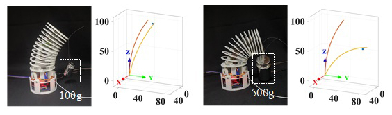
However, the parabolic model we proposed, combined with the real-time update of the attitude data collected by the micro-inertial sensor, can accurately capture the external interference information that causes the flexible arm to bend and evaluate the shape of the flexible arm in real time. Figure 11 shows the actual bending state of the flexible arm under loads of 100 and 500 g, as well as the shape estimation curves of the constant-curvature assumption and the parabolic method. It is shown that the shape estimation curve of the parabolic assumption matches the actual bending shape of the flexible arm, with the error increasing only from 3.08 mm under a 100 g load to 11.38 mm under a 500 g load. While the shape prediction curve obtained by the constant-curvature method gradually deviates from the actual bending shape of the flexible arm as the load increases, and the estimation error also increases from 9.77 mm under a 100 g load to 56.57 mm under a 500 g load.

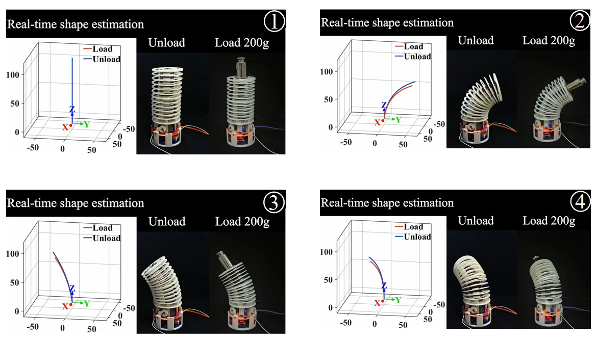
Considering that external end payload induces additional deformation of the flexible spine, and fine motion control of flexible arms poses inherent challenges, dynamic comparative experiments are conducted under two scenarios: end effector loaded with a 200 g mass and fully unloaded. The identical second flexible arm prototype adopted in static loading tests is reused here. The flexible segment has an initial length of 114.5 mm under unloaded conditions and contracts to 104.5 mm after mounting the 200 g payload. The flexible arm executes omnidirectional 360° rotation about the vertical axis with identical actuation speed for both loading cases, and full experimental procedures are recorded. Representative key frames are presented in Fig. 12.

Table 4 Key parameters of hyper-redundant manipulator.

Qualitative observation reveals that the flexible arm maintains stable fine motion without abrupt morphological deformation under end loading, which validates the rationality of the mechanical design. For both loaded and unloaded cases, predicted shape curves match well with actual bending configurations. This demonstrates that the proposed shape prediction method is applicable to real-time morphological reconstruction of flexible arms under payload conditions.

To quantitatively evaluate the real-time dynamic performance of the estimation algorithm, estimation latency and convergence time are measured on the embedded controller during the above dynamic experiments. Estimation latency denotes the time interval from receiving a frame of inertial sensor data to outputting the complete 3D shape curve; convergence time refers to the duration required for estimation error to fall within the allowable error band after the flexible arm undergoes a posture change. Statistical results are summarized in Table 3. The average single-step estimation latency reaches 8 ms with the maximum value of 12 ms, both well below the 20 ms sampling period, so the algorithm completes the computation of one frame within the period, before the next frame arrives. The convergence time, which characterizes the transient settling of the estimator after a posture change rather than a single computation step, averages 21 ms with a maximum of 32 ms, i.e., approximately one to two sampling periods; such a transient is inherent to recursive shape estimation and is fully compatible with the closed-loop perception requirement at the given sampling rate. These results together verify that the proposed modeling approach possesses sufficient real-time performance for dynamic closed-loop shape perception under loaded working conditions.

Figure 13 Real-time shape estimation under a large-amplitude undulating motion mode.

Figure 14 Real-time shape estimation under a small-amplitude undulating motion mode.

To further clarify the comprehensive advantages of the proposed method, a qualitative comparison with state-of-the-art shape estimation approaches is discussed herein. Compared with recent IMU-based shape reconstruction methods that still adopt constant-curvature assumptions, the proposed parabolic model effectively characterizes the non-uniform quadratic bending of spring flexible spines under external loads, achieving significantly lower drift and higher adaptability under varying disturbances. In contrast to vision-based shape estimation techniques that rely on external cameras and are susceptible to occlusion, darkness and narrow-space limitations, the fully inertial sensing framework maintains stable perception capability in unstructured and confined environments. Different from learning-assisted data-driven methods that require massive labeled datasets and suffer from poor generalization under unseen loading conditions, this physics-driven parabolic model possesses clear geometric interpretability and does not rely on training data, while achieving high precision and real-time performance. Therefore, the proposed method achieves a better balance of accuracy, environmental adaptability, anti-disturbance ability and computational practicability compared with existing mainstream shape estimation strategies.

4.4 The motion test under the plane bending condition

To verify the comprehensive performance of the shape estimation method for the continuum snake robot based on distributed micro-inertial sensors, three motion modes were designed for verification experiments, including (1) a large-amplitude undulating motion mode, which is used to achieve the robot's turning or obstacle crossing; (2) a small-amplitude undulating motion mode, which is used for the robot to pass through narrow environments; (3) a smooth gait transition mode, which is used for the mutual switching between the large-amplitude undulating motion and the small-amplitude undulating motion. The experimental prototype is the five-module serial continuum snake robot introduced in the second part. During the large-amplitude undulation, the undulation curve wavelength is approximately equal to the length of four flexible arm modules and the maximum amplitude is about 100 mm. During the small-amplitude undulation, the wavelength is approximately equal to the length of two flexible arm modules and the maximum amplitude is about 50 mm. The main controller collects and processes data from all modules at a frequency of 20 Hz. The shape of the soft robotic system is calculated based on Eqs. (37) and (38).

Figure 13 shows the comparison between the real-time shape estimation curve and the actual motion state of the snake-like robot during its large-amplitude meandering motion on a plane. Three characteristic moments (corresponding to the maximum positive amplitude, straight line and maximum negative amplitude, respectively) were selected, and the true and estimated values of the positions of the five module ends at each moment were extracted. It is shown that the real-time shape estimation curve is in good agreement with the actual motion state of the snake-like robot. The root-mean-square error (RMSE) at each moment during the motion of the snake-like robot was further calculated. The results show that the error value increases with the increase in the bending amplitude, reaching approximately 15.7 mm at the maximum amplitude and decreasing to 3.2 mm in the straight state. This indicates that the estimation error in the end points of each module fluctuates more significantly under strong bending, which is consistent with the nonlinear deformation of the flexible spine and the amplification effect of sensor noise under dynamic conditions.

Figure 15 Real-time shape estimation from large-curvature to small-curvature undulation state.

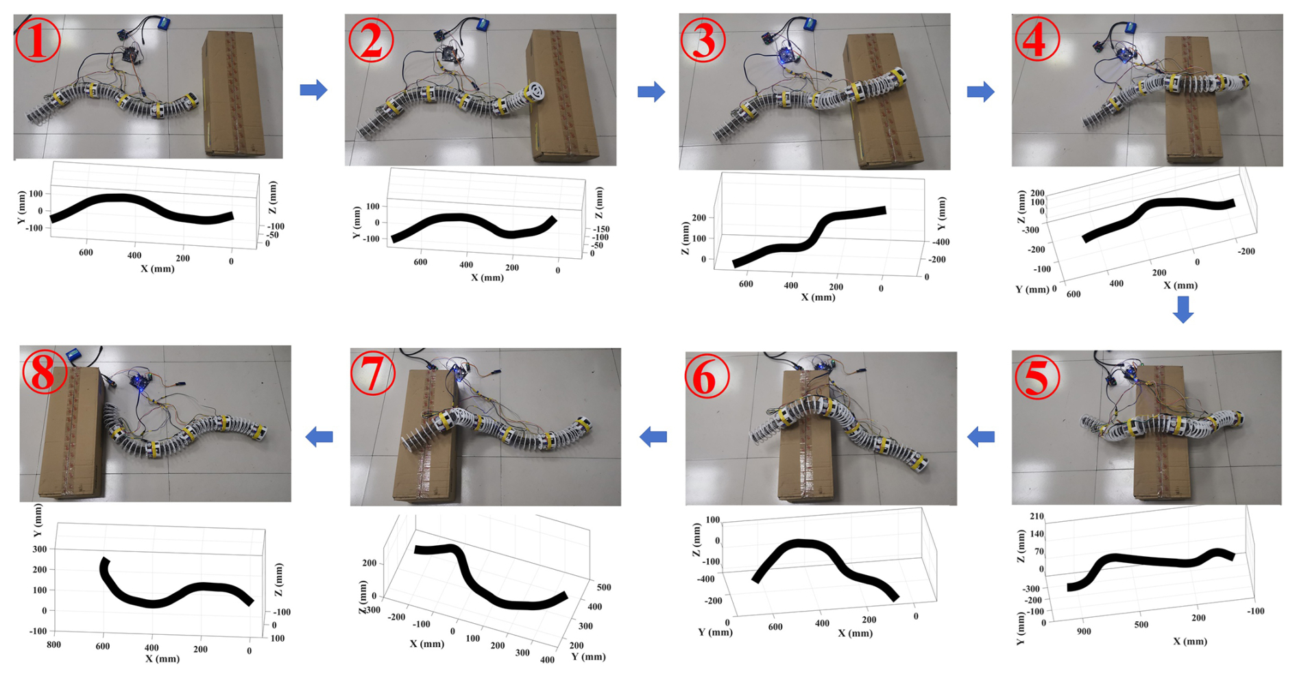
Figure 16 Obstacle crossing test of snake robot obstacle crossing and corresponding 3D estimated shape curves.

Figure 14 shows the small-amplitude undulating motion mode of the snake-like robot. Similar to the large-amplitude undulating gait, three characteristic moments in the motion cycle are selected to compare the real-time shape estimation curve with the actual motion state. It is shown that the waveform characteristics obtained by shape prediction are consistent with the periodic changes in the robot's shape, indicating that the shape estimation method can effectively track the robot's periodic motion. In addition, the shape estimation errors at each moment were calculated. The results show that the average RMSE at the three moments is 5.3 mm, with the errors at the wave peaks and troughs being slightly larger at 7.3 mm and the error in the near-straight state being the smallest at 3.6 mm. Compared with the large-amplitude undulating motion in Fig. 13, whose average RMSE is approximately 9.62 mm, the overall shape prediction error in the small-amplitude undulating motion is reduced by approximately 44.9 % to an average RMSE of 5.3 mm. This indicates that the parabolic model has higher fitting accuracy under smaller amplitude conditions.

To verify the adaptability of the proposed shape estimation method in the gait reconstruction process, a sampling analysis was conducted on a continuous transition process ranging from large-amplitude wiggling to small-amplitude wiggling. As shown in Fig. 15, it is a comparison chart of the estimated shape and the actual state of the snake-like robot at three equally spaced moments along the transition path. It is shown that in the initial stage of the transition, the difference between the estimated shape and the actual motion state is significant, mainly due to the lag in the dynamic response of the flexible spine and the control delay. Later, the two gradually converge, verifying the continuous adaptability of the proposed method to different curvature movements.

4.5 Obstacle crossing test under non-ideal contact condition

To evaluate the performance of the proposed pose estimation and adaptive error compensation strategy under non-ideal unstructured scenarios, rigid obstacle crossing experiments are conducted, where contact force and friction between robot and obstacle introduce extra disturbance to the built-in inertial sensors. The whole obstacle crossing procedure is split into eight sequential motion stages, with real robot configurations and corresponding 3D estimated shapes illustrated in Fig. 16. The root-mean-square estimation error in each stage is plotted in Fig. 17. Stages 2 and 7 produce larger RMSE values (19.4 mm, 16.5 mm) because the flexible arm bears strong extrusion and friction from the obstacle at these two moments, leading to obvious inertial sensor drift; for other stages with mild contact, the estimation error remains below 13 mm.

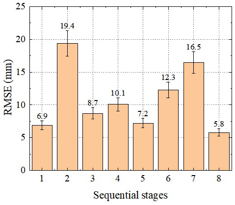
Figure 17 Root-mean-square error in the eight sequential stages during the obstacle crossing test.

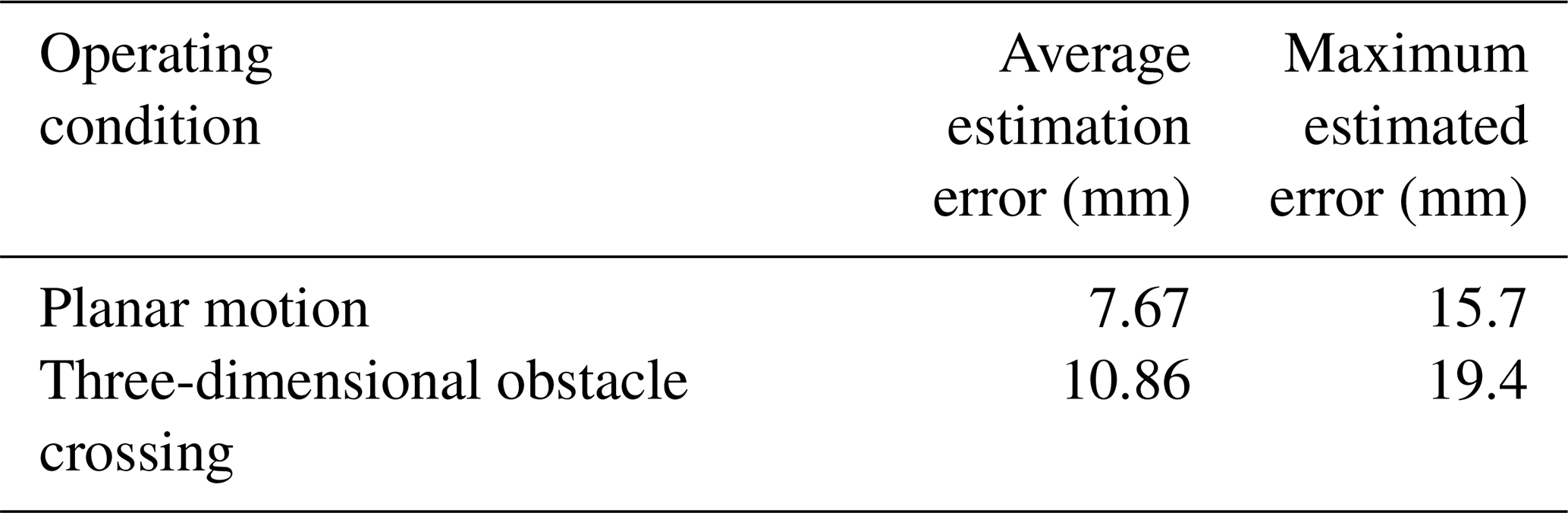
Table 4 further compares the overall estimation performance between free planar motion and three-dimensional obstacle crossing. Under obstacle contact disturbance, the average estimation error rises from 7.67–10.86 mm and the maximum error increases from 15.7–19.4 mm. Although external contact disturbance deteriorates raw inertial measurement precision, the embedded online adaptive compensation keeps estimation error within an acceptable engineering range. This set of experiments verifies that the parabolic pose estimation framework with error compensation possesses satisfactory robustness for unstructured environments with protruding obstacles. Future work will carry out tests on granular rough ground to further extend application scenarios.

5 Conclusion

A modular continuum snake-like robot with a three-spring twisted flexible spine and triple-cable actuation system is designed to balance structural compliance and motion controllability. A parabolic deformation modeling framework is further established, which fuses attitude data from distributed micro-inertial sensors to achieve real-time three-dimensional morphological reconstruction of the flexible robot. Different from conventional constant-curvature models, the proposed scheme removes the rigid constraint of fixed curvature variation, enabling accurate depiction of diverse bending configurations.

The core innovations of this work are summarized as follows. Firstly, the modular layout integrates driving, sensing and control subsystems inside each unit, allowing omnidirectional bending and axial length regulation. Relative to monolithic continuum robots, this modular design improves system scalability, maintainability and environmental adaptability for complex terrain. Secondly, the parabolic deformation assumption faithfully reproduces the actual bending profile of the spring backbone, delivering superior modeling accuracy compared with constant-curvature approaches widely adopted in existing IMU-based continuum robot shape estimation. This constitutes the primary methodological advance over mainstream inertial sensing and geometric modeling schemes. Compared with vision-based reconstruction and learning-assisted data-driven estimation methods, the fully inertial framework eliminates the environmental occlusion limitations of optical sensors and avoids the massive labeled dataset requirements of black-box learning models, achieving a balanced trade-off among precision, environmental adaptability and real-time computational efficiency. To mitigate systematic measurement deviations originating from assembly tolerances and non-uniform external loads, a sensor position offset compensation strategy incorporating batch benchmark calibration and lightweight online adaptive tuning is proposed, which effectively suppresses time-varying inertial drift. Finally, static and dynamic loading tests verify that the endpoint positioning error in an individual flexible module is restricted within 3 %. Comprehensive multi-gait experiments covering free planar bending and rigid obstacle-crossing scenarios show that the average root-mean-square error in three-dimensional shape estimation remains below 11 mm, which strongly demonstrates the precision and robustness of the integrated modeling pipeline.

Notwithstanding the above merits, two critical limitations of the current study are identified. For one thing, the parabolic approximation holds only for quasi-static deformation with small-to-medium bending amplitudes; significant estimation degradation will emerge under extreme large bending angles, intense inertial shocks and heavy transverse external forces. For another, all experimental validations are conducted on flat ground and rigid obstacle platforms. Sufficient tests on granular rough terrain, muddy surfaces and long-duration cyclic operation are absent, and the long-term sensor drift triggered by spring creep and cable relaxation has not been quantitatively characterized.

Corresponding future research directions are put forward to address the aforementioned deficiencies. First, a unified hybrid parabolic–catenary deformation model will be developed to accommodate large bending deformation and complex multi-source loading states. Second, field experiments on granular, uneven terrain will be supplemented, and visual-inertial fusion perception will be introduced to further attenuate inertial measurement disturbances. Third, autonomous gait-planning algorithms will be coupled with the real-time shape estimation framework to support autonomous reconnaissance missions in unstructured pipelines and post-collapse ruins.