An enhanced neural network-based method for predicting step error in a five-axis finishing machining

To address the low efficiency of traditional geometry-based step error calculations in five-axis numerical control (NC) finishing that cannot reuse historical data, this study proposes a step error prediction method based on a SSA-Attention-LSTM (Sparrow search algorithm–attention mechanism–long short-term memory) model. The method employs principal component analysis (PCA) for dimensionality reduction, optimizes LSTM hyperparameters using the Sparrow search algorithm, incorporates an attention mechanism to enhance key feature extraction, and introduces dropout to prevent overfitting. Experimental results on two surface models show that the proposed model achieves an average R² of 99.4 %, which is 31 %, 10 %, 5 %, and 6 % higher than that of back propagation (BP), long short-term memory (LSTM), bidirectional gated recurrent unit (BiGRU), and bidirectional long short-term memory (BiLSTM) models. In the blade test case, the model achieves high-precision prediction using only 9480 training samples, with an R² of 0.995, demonstrating high prediction accuracy for step error in five-axis finishing tool paths.

1 Introduction

Five-axis computer numerical control (CNC) machining is widely applied in the precision machining of complex free-form surfaces. As shown in Fig. 1a, the cutting path of the tool along the discrete cutter contact (CC) points on the workpiece surface is illustrated, while Fig. 1b shows the step error formed between adjacent cutter location (CL) points. Taking the jth and (j+1)th CL points on the ith tool path as an example, the tool holding points are O_i,j and $O_{i,j+\mathrm{1}}$, respectively. The maximum normal distance $e_{max}^{\mathrm{L}}$ between the CC point line $P_{i,j}^{\mathrm{CC}}{P}_{i,j+\mathrm{1}}^{\mathrm{CC}}$ and the ideal CC point trajectory CC_i,j is defined as the linear error. Taking the midpoint O_m of the line segment O_i,j and $O_{i,j+\mathrm{1}}$, the maximum normal distance $e_{max}^{\mathrm{NL}}$ among the tool base circle at O_m, the CC point line $P_{i,j}^{\mathrm{CC}}{P}_{i,j+\mathrm{1}}^{\mathrm{CC}}$, and the ideal CC point trajectory, CC_i,j is defined as the nonlinear error, where $P_{\mathrm{m}}^{\mathrm{CL}}$ is the CC point coordinate corresponding to the midpoint of the CL points, while T_m represents the intermediate tool axis vector obtained by averaging and normalizing T_i,j and ${\mathit{T}}_{i,j+\mathrm{1}}$.

Figure 1 Tool cutting and step error. (a) Tool cutting along CC points. (b) Step error between two adjacent CL points.

When the tool completes the five-axis simultaneous motion from $P_{i,j}^{\mathrm{CL}}$ to $P_{i,j+\mathrm{1}}^{\mathrm{CL}}$, the tool envelope surface formed by the sweeping cutting edge (i.e., the edge of the tool base circle) constitutes the actual cutting path. The maximum normal distance e_max between this actual cutting path and the ideal CC point trajectory line CC_i,j is defined as the step error, which is a key geometric indicator for controlling machining accuracy.

Currently, step error calculation mainly relies on geometry-based iterative methods. Various approaches have been proposed, such as point-by-point iteration by Liu et al. (2022), dynamic-programming-based tool path planning by Wu et al. (2008), and geometric envelope methods by Zhou et al. (2015). These geometry-based iterative methods require explicit mathematical models, and their computational cost increases sharply with higher-precision requirements. Moreover, each calculation is performed independently without reusing historical experience, resulting in low efficiency when generating high-quality tool paths that require massive step error calculations, which has become a major bottleneck limiting their practical application.

In recent years, machine learning techniques have shown potential in tool path planning due to their ability to learn from data and handle complex nonlinear relationships. Neural networks have been applied to personalized tool path generation, machining error prediction, tool path length prediction, and machining cycle prediction (Eskandari et al., 2013; Geng et al., 2011; Sun et al., 2022). Zhang et al. (2023) proposed using a back propagation (BP) neural network to predict three-axis step error with high accuracy. However, it suffers from issues such as slow computation and susceptibility to overfitting, making it difficult to directly apply to five-axis step error prediction.

Besides the machining field, data-driven methods are also widely applied in dynamic system analysis and intelligent monitoring. Existing studies have established 3D vision systems to realize non-contact detection of equipment (Cascino et al., 2025), and other studies have utilized deep learning to complete mechanical component defect recognition (Zheng et al., 2021). The above cross-domain studies confirm that deep neural networks excel at mining nonlinear features from high-dimensional data, providing a good reference for the step error prediction research in this paper.

To address the above problems, this paper proposes a step error prediction method for five-axis NC finishing based on the SSA-attention-LSTM (Sparrow search algorithm–attention mechanism–long short-term memory) model. By integrating the Sparrow search algorithm (SSA) for hyperparameter optimization and incorporating an attention mechanism to enhance key feature extraction, the model effectively captures the spatiotemporal continuity and nonlinear characteristics of tool motion, thereby improving prediction accuracy and stability while preventing overfitting. In order to use the SSA-attention-LSTM model to predict five-axis finishing step error, this paper conducts research on data preprocessing architecture design, network structure optimization, and multi-task collaborative training mechanisms. The main content is as follows: Sect. 2 defines the step error based on five-axis machining geometric principles. Section 3 designs the sample data architecture. Z-score standardization is applied to eliminate unit differences (Al-Faiz et al., 2018). Principal component analysis (PCA) is used for dimensionality reduction and reconstruction of high-dimensional discrete point sets to compress redundant noise and enhance model generalization capability (Fariz and Basha, 2024). Section 4 constructs the SSA-attention-LSTM collaborative optimization framework. The SSA is introduced to dynamically optimize LSTM hyperparameters (hidden-layer dimensions, learning rate). The attention mechanism is used to weight and focus on key CC and CL features. Dropout (Chen et al., 2024) regularization and the Adam (Kingma and Ba, 2014; Salem et al., 2022) optimizer are combined to suppress overfitting. Section 5 validates the effectiveness and prediction accuracy of the proposed SSA-attention-LSTM model using tool path sample data from two general free-form surfaces and a typical aero-engine blade workpiece, covering both basic geometric test cases and practical industrial scenarios.

2 Sample data design and optimization

This paper employs tool parameters and CC and CL points as core input variables. As the samples contain diverse parameter types (e.g., tool radius, point coordinates), standardization is applied to unify the scales of these parameters. The high-dimensional features of the standardized samples are reconstructed by PCA to reduce the dimensionality, aiming to eliminate interference from redundant features and retain critical ones, thereby suppressing model overfitting.

2.1 Sample data design

Before using the neural network model for step error prediction, extensive samples are required to train the model for ideal prediction accuracy. As derived from the geometric principles of step error, the following parameters are all necessary input variables for calculating five-axis step error: adjacent CC points ($P_{i,j}^{\mathrm{CC}}$, $P_{i,j+\mathrm{1}}^{\mathrm{CC}}$), CL points ($P_{i,j}^{\mathrm{CL}}$, $P_{i,j+\mathrm{1}}^{\mathrm{CL}}$) and their corresponding tool axis vectors (T_i,j, ${\mathit{T}}_{i,j+\mathrm{1}}$), the discrete point set $\left\{P_k^{i,j}\right\}$ on the local CC curveCC_i,j, and basic tool parameters. These data collectively constitute the input features of the samples, while the step error value is the only output variable. They form the sample data structure shown in Table 1.

Table 1 Sample data required for step error prediction.

2.2 Sample data optimization

In step error prediction of the five-axis finish machining, original sample data suffer from high-dimensionality, multi-dimensional units, and redundant features, which directly impair the model's computational efficiency and generalization capability. To address this, this section proposes an optimization strategy based on data standardization and PCA. Z-score standardization is applied to eliminate parameter-scale discrepancies, and PCA extracts critical geometric features and compresses redundant information. This approach effectively reduces data complexity, suppresses noise interference, and significantly enhances the model's prediction efficiency and accuracy.

3 Design and optimization of the SSA-attention-LSTM model for step error prediction

To achieve high-precision and high-efficiency prediction of step error for five-axis finishing tool paths, this paper proposes a joint modeling and optimization method that integrates the SSA with an attention-mechanism-based LSTM network, resulting in the SSA-attention-LSTM model. The attention mechanism is introduced to adaptively highlight key CL point features and suppress attenuation and noise in information transmission. Furthermore, the SSA algorithm is integrated to achieve intelligent global optimization of hyperparameters, enhancing the model's generalizability while avoiding local optima caused by complex sample features, thereby significantly improving the model's prediction robustness and accuracy.

3.1 Design of the LSTM model integrated with attention mechanism

Unlike traditional BP neural networks that process independent samples, LSTM, as an improved architecture of recurrent neural networks (RNNs), introduces gating mechanisms (forget gate, input gate, and output gate). The forget gate determines the retention level of important historical CC and CL points, preserving crucial features. The input gate then integrates subsequent CC and CL point features for comprehensive learning of core sample characteristics. Finally, the output gate extracts the final core sample data from the memory cell. This mechanism incorporates historical sample information for step error prediction, combines current outputs with hidden states from previous time steps, and enable perception and transmission of continuous contextual features.

For five-axis finishing tool paths, this mechanism allows the model to incorporate preceding tool path information and model temporal correlations of step error, thus improving prediction accuracy and stability. However, LSTM may insufficiently distinguish feature importance, and early CL point information is prone to attenuation during transmission, reducing prediction accuracy. Therefore, an attention mechanism is introduced to optimize LSTM by dynamically weighting different features according to their importance, thereby achieving superior prediction results.

Figure 2 Attention-LSTM structure.

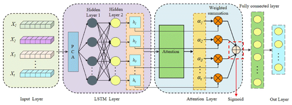
As shown in Fig. 2, the attention-LSTM model structure comprises five layers: input layer, LSTM layer, attention layer, fully connected (FC) layer, and output layer. The input layer imports preprocessed sequence data into the LSTM layer for model training. It should be emphasized that the lead angle is used as an independent input feature in this study, and all information of the tilt angle is completely contained in the two three-dimensional tool axis vectors. As a complete representation of spatial posture, the tool axis vector can eliminate the inherent periodic non-uniqueness of angle parameters and retain the inherent coupling relationship between posture angles, which is more conducive to network learning.

After learning sample features through the LSTM layer, the hidden states h_t at all time steps are output. Subsequently, an independent attention layer processes these hidden states; this layer calculates corresponding weight coefficients α_t for each hidden state h_t and continuously updates these weights to emphasize the information most critical for prediction. Finally, nonlinear transformation of the weighted feature vector is performed via a sigmoid activation function. Features are mapped through the FC layer, and prediction is completed at the output layer.

The weight coefficient α_t is calculated in Eq. (1). h_t represents the hidden state at the tth time step. w is a learnable weight matrix. b and u represent the learnable bias vector and weight vector, respectively. e_t represents the attention score at time step t. α_t indicates the relative importance of the hidden state h_t at the tth time step to the current prediction task, i.e., the weight coefficient.

$$\begin{array}{}\text{(1)}& \left\{\begin{array}{l}{e}_t={\mathit{u}}^T\tanh (\mathbf{w}{h}_t+\mathit{b})\\ {\mathit{\alpha }}_t=\frac{\exp \left(e_t\right)}{{\sum }_{j=\mathrm{1}}^{T{\sum }_j}\exp }\end{array}\right.\end{array}$$

After calculating the weight coefficients, as shown in Eq. (2), a vector v that integrates global key feature information is obtained by performing a weighted summation of the hidden states across all time steps. This vector encompasses the historical information most critical to the current prediction.

$$\begin{array}{}\text{(2)}& \mathit{v}={\sum }_{t=\mathrm{1}}^T{\mathit{\alpha }}_t{h}_t\end{array}$$

Finally, a fully connected layer is set at the output layer. The vector v, which integrates global key feature information, is mapped into the final predicted value $\widehat{y}$, as shown in Eq. (3). Here, W_o represents the output layer weight matrix, b_o represents the output layer bias vector, and σ represents the Sigmoid activation function.

$$\begin{array}{}\text{(3)}& \widehat{y}=\mathit{\sigma }\left({\mathbf{W}}_{\mathrm{o}}\mathit{v}+{\mathit{b}}_{\mathrm{o}}\right)\end{array}$$

3.2 Attention-LSTM hyperparameter optimization based on SSA algorithm

In five-axis machining step error prediction tasks, input features within the dataset exhibit strong correlations. Consequently, minor variations in hyperparameters (e.g., LSTM hidden layer dimensions, learning rate) can cause significant fluctuations in prediction accuracy. Furthermore, when machined surface profiles are similar, the distribution of key feature points (CC, CL) may overlap, which can easily trap the training model in local optima. To address this, this section uses the SSA for the collaborative optimization of the LSTM neural network.

The SSA is a swarm intelligence optimization algorithm that simulates the foraging and anti-predation behaviors of sparrows. By mimicking sparrows' food-seeking and danger avoidance behaviors, it balances global and local search, effectively escaping local optima to find the global optimal solution. As shown in Fig. 3, the main steps of the algorithm include setting hyperparameter boundaries, population initialization, producer assignment, scrounger assignment, and scout assignment. After each position update, the fitness value of each individual is calculated. The optimal solution is updated, and the termination condition is assessed based on fitness. The detailed steps are as follows.

Figure 3 SSA framework process.

3.2.1 Step 1: hyperparameter boundary setting and population initialization

In the initial phase of SSA, the search space is firstly defined, and an initial candidate solution set is generated to establish a start point for subsequent iterative optimization. The population size is N. As shown in Eq. (4), each sparrow's position vector X_i corresponds to a candidate solution, where ${\mathit{X}}_i=[x_{i\mathrm{1}},x_{i\mathrm{2}},\mathrm{\dots },x_{iD}]$ represents the position vector of the ith sparrow in the D-dimensional search space. Ub and Lb are the upper- and the lower-bound vectors of the hyperparameters, respectively. The symbol ⊙ denotes element-wise multiplication, and rand(0,1) represents a randomly generated vector with a uniform distribution in the interval [0,1].

$$\begin{array}{}\text{(4)}& {\mathit{X}}_i=\mathrm{Lb}+\mathrm{rand}(\mathrm{0},\mathrm{1})\odot (\mathrm{Ub}-\mathrm{Lb}),i=\mathrm{1},\mathrm{2},\mathrm{\dots },N\end{array}$$

3.2.2 Step 2: fitness value calculation and producer assignment

1. Fitness value calculation.

   The fitness values of the initially selected population are calculated separately. The individual fitness value f(X_i) for X_i is calculated by Eq. (5), where M is the number of validation set samples, y_j is the true value of the jth sample, and (X_i) is the predicted value of thejth sample by the model using hyperparameters X_i.

   $$\begin{array}{}\text{(5)}& f\left({\mathit{X}}_i\right)={\displaystyle \frac{\mathrm{1}}{M}}{\sum }_{j=\mathrm{1}}^M{\left(y_j-{\widehat{y}}_j\left({\mathit{X}}_i\right)\right)}^{\mathrm{2}}\end{array}$$

2. Producer selection.

   To guide the population to search in better regions, leaders with exploration capability, named “producers”, are selected from the current population. The calculated fitness values are sorted in ascending order (since the fitness value is MSE, a smaller value indicates a better solution). As shown in Eq. (6), the top p_n individuals are selected as producers P to guide the optimal hyperparameter search direction, where rank() sorts f(X_i) in ascending order.

   $$\begin{array}{}\text{(6)}& P=\mathit{\{}{\mathit{X}}_i\left|\mathrm{rank}\left(f\right({\mathit{X}}_i\left)\right)\le p_n\right.\end{array}$$

3. Producer position update.

   When producers perform global search, both extensive exploration and refined local search are expected. In Eq. (7), ${\mathit{X}}_i^{t+\mathrm{1}}$ reflects the real-time update of the producer's position. t is the current iteration count. T is the maximum number of iterations. α represents a random decay factor. R₂ is the alert value. If R₂ is less than the safety threshold ST, refined local search is performed. Otherwise, extensive global search is conducted. $\mathit{Q}\sim N(\mathrm{0},\mathrm{1})$ is a random vector following the standard normal distribution, and L is an all-one vector.

   $$\begin{array}{}\text{(7)}& {\mathit{X}}_i^{t+\mathrm{1}}=\left\{\begin{array}{ll}{\mathit{X}}_i^t\odot \exp \left(-\frac{i}{\mathit{\alpha }\cdot T}\right)& R_{\mathrm{2}}<\mathrm{ST}\\ {\mathit{X}}_i^t+Q\cdot L& R_{\mathrm{2}}\ge \mathrm{ST}\end{array}\right.\end{array}$$

3.2.3 Step 3: scrounger assignment

During the producers' optimization process, scroungers will follow the producers for local optimization. As shown in Eq. (8), utilizing known high-quality regions and information, the first half of scroungers $(i>pN/\mathrm{2})$ move toward the optimal producer direction, while the latter half move away from the worst region to avoid inferior solutions. In Eq. (9), $X_{\mathrm{P}}^t$ represents the current optimal producer position. $X_{\mathrm{worst}}^t$ represents the current worst position. A is a random matrix of ±1, and i is the individual ranking index.

$$\begin{array}{}\text{(8)}& {\mathit{X}}_i^{t+\mathrm{1}}=\left\{\begin{array}{ll}{X}_{\mathrm{P}}^t+|{\mathit{X}}_i^t-X_{\mathrm{P}}^t|\cdot A^{+}\cdot L& i>\frac{pN}{\mathrm{2}}\\ Q\cdot \exp \left(\frac{X_{\mathrm{worst}}^t-{\mathit{X}}_i^t}{i^{\mathrm{2}}}\right)& i\le \frac{pN}{\mathrm{2}}\end{array}\right.\end{array}$$

3.2.4 Step 4: scout assignment

To enhance the algorithm's global search capability and prevent the population from falling into local optima during the optimization process, the SSA algorithm sets a portion of individuals as “scouts”. Scouts execute two different position update strategies based on their current status, with the mathematical expression shown in Eq. (9).

Firstly, when the fitness is not optimal (i.e., f_i≠f_g), it indicates that the individual is still in a potentially valuable non-optimal region. In this case, its position update strategy is to move toward the current global best position $X_{\mathrm{best}}^t$. This is achieved by adding a random step size factor $\mathit{\beta }\cdot |{\mathit{X}}_i^t-X_{\mathrm{best}}^t|$, enabling local refined search and thereby enhancing the algorithm's convergence capability.

Secondly, when an individual's fitness reaches the global optimum (i.e., f_i=f_g), it means the individual may be trapped in a local optimum. To break this stagnation and increase the diversity of hyperparameter solutions, its update strategy shifts to an adjustment based on the global worst position $X_{\mathrm{worst}}^t$. Specifically, this is implemented by introducing a proportional term $K\cdot \frac{|{\mathit{X}}_i^t-X_{\mathrm{worst}}^t|}{f_i-f_w+\mathit{ϵ}}$, which incorporates a random step size factor K and the fitness difference between the current individual and the worst individual (a minimal constant ϵ is added to prevent the denominator from being zero and ensure numerical stability). This prompts the individual to escape the current optimal region and explore a wider solution space.

Finally, the fitness is recalculated based on the updated positions, and it is checked whether the termination conditions are met.

$$\begin{array}{}\text{(9)}& {\mathit{X}}_i^{t+\mathrm{1}}=\left\{\begin{array}{ll}{X}_{\mathrm{best}}^t+\mathit{\beta }\cdot |{\mathit{X}}_i^t-X_{\mathrm{best}}^t|& f_i\ne f_{\mathrm{g}}\\ X_{\mathrm{best}}^t+K\cdot \frac{|{\mathit{X}}_i^t-X_{\mathrm{worst}}^t|}{f_i-f_w+\mathit{ϵ}}& f_i=f_{\mathrm{g}}\end{array}\right.\end{array}$$

3.3 Algorithm implementation

After sample construction, preprocessing is performed using Z-score normalization and PCA dimensionality reduction. Temporal features are extracted via LSTM, followed by an attention mechanism to enhance key features. Hyperparameters are optimized using SSA, and the model is trained with the Adam optimizer, early stopping, and dropout to output the predicted step error. The detailed algorithm steps are as follows.

3.3.1 Step 1: data import and standardized preprocessing

Sample data are imported, including tool parameters (radius R, length L, inclination angle α), as well as discrete CC and CL points. The dataset is then batch-normalized by the Z-score standardization method described in Sect. 2.2.1.

3.3.2 Step 2: PCA dimensionality reduction and reconstruction

To eliminate redundant noise in high-dimensional data, PCA as described in Sect. 2.2.2 is applied to the standardized data for dimensionality reduction, and the reduced-dimensional output is generated.

3.3.3 Step 3: configure LSTM layer for temporal feature extraction

An LSTM network is used to extract continuous features from CC and CL point coordinates, learning the dependency relationships between adjacent CL points.

3.3.4 Step 4: configure attention mechanism layer

Following the method described in Sect. 3.1, an attention module is designed to weight the hidden states output by the LSTM, achieving adaptive weight allocation to reinforce key CC and CL point features.

3.3.5 Step 5: implement SSA for hyperparameter optimization

As outlined in Sect. 3.2, the hyperparameters (e.g., hidden layer dimensions, learning rate) for the attention-LSTM model are initialized. The global exploration and local exploitation mechanisms of SSA are utilized to iteratively optimize the hyperparameter combinations, avoiding local optima and enhancing the model's generalization capability.

3.3.6 Step 6: configure Adam optimization and dropout regularization layer

To mitigate issues such as local optima and slow convergence in gradient descent, the Adam optimizer is employed. A dropout algorithm is incorporated before the fully connected output layer to randomly discard outputs from some neurons, suppressing interference from non-critical parameters and reducing the risk of noise-induced overfitting during training.

3.3.7 Step 7: error evaluation and model output

The predicted step error values output by the model are compared with the true values generated by the geometric iterative method (Liu et al., 2012) and the mean squared error (MSE) is calculated to verify the model's prediction accuracy. If the MSE meets the predefined threshold, the model is considered to be optimized, and the predicted step error values are accepted as final outputs. Otherwise, the model parameters are further refined through backpropagation and iterative training until the convergence criterion is satisfied. The optimized model is then deployed for high-precision step error prediction.

4 Case study

4.1 Sample generation

The two surface models S1 and S2 shown in Fig. 4 are imported into the CAM software developed for this study. Iso-parameter tool paths are generated with 99 and 100 lines respectively, each containing 150 and 200 CL points, respectively. The machining tool is a flat-end cutter with fillet radius of 0 mm, a radius R of 5 mm, and a length L of 50 mm. The inclination angle α is 15°.

Figure 4 Two surfaces.

Table 2 Parameter and sample statistics table.

While generating tool paths, six-dimensional features are collected between two adjacent CC points following the sample structure defined in Sect. 2.1, including 4 basic tool parameters, 30 features from 10 discrete CC points (3D coordinates for each point), 3 features from the 3D coordinates of the first CL point, 3 features from the corresponding tool axis vector of the first CL point (represented by x, y, and z values), 3 features from the tool axis vector of the second adjacent CL point, and 3 features from the 3D coordinates of the second CL point. These 46-D features constitute the input of each sample, while the corresponding step error value is the output. The true values of step error are calculated by the geometric method (Liu et al., 2020) during tool path generation. Their ranges for Surface S1 and S2 samples are [−24 µm, −6 µm] and [−4 µ m, −1 µm], respectively. All sample data are constructed according to the sample structure in Table 1 and exported to txt files. The detailed parameter settings and sample statistics for both surfaces are summarized in Table 2. A total of 80 % of the samples are randomly selected to form the training set, and the remaining samples form the test set.

4.2 Algorithm verification and comparison

This section uses the mean squared error (MSE) and coefficient of determination (R²) in Eq. (10) to evaluate the prediction performance of the model by quantifying the error between the predicted step error values and the true values, where N denotes the total number of test samples, ${\widehat{y}}_t$ represents the predicted step error value (in µm), y_t is the corresponding true step error value (in µm), and $\stackrel{\mathrm{‾}}{y}$ denotes the mean value of all true step error values (in µm). A smaller MSE (in µm²) and an R² (dimensionless) closer to 1 indicate higher prediction accuracy.

$$\begin{array}{}\text{(10)}& \left\{\begin{array}{l}\mathrm{MSE}=\frac{\mathrm{1}}{N}{\sum }_{t=\mathrm{1}}^N{\left({\widehat{y}}_t-y_t\right)}^{\mathrm{2}}\\ \\ R^{\mathrm{2}}=\mathrm{1}-\frac{{\sum }_{t=\mathrm{1}}^N{\left(y_t-{\widehat{y}}_t\right)}^{\mathrm{2}}}{{\sum }_{t=\mathrm{1}}^N{\left(y_t-\stackrel{\mathrm{‾}}{y}\right)}^{\mathrm{2}}}\end{array}\right.\end{array}$$

This section introduces three widely used regression models: the BP neural network, BiGRU, neural network and BiLSTM neural network (Liu et al., 2017, 2016), along with an unoptimized LSTM model and the proposed SSA-attention-LSTM model for step error prediction. The prediction results of each model are compared. The SSA algorithm is employed to optimize the neural network hyperparameters: learning rate (lr), number of neurons in hidden layer 1 (lstm1), number of neurons in hidden layer 2 (lstm2), and training epochs. The optimized values are shown in Table 3.

Table 3 Hyperparameters of SSA-attention-LSTM.

4.2.1 Comparison of SSA-attention-LSTM with mainstream network models

Samples from surfaces S1 and S2 were used to train the BP, LSTM, BiGRU, BiLSTM, and the proposed SSA-attention-LSTM neural network models, respectively. During training, the loss value of the proposed model decreased rapidly within the first 100 epochs and then stabilized, leading to early termination upon meeting the stopping criterion. In terms of computational efficiency, the proposed method demonstrates superior performance, with the geometric iterative method requiring 12.261 s to calculate step errors for 14 850 CL points, while the neural network prediction completes in just 3.6 s. The MSE and R² values of the five neural network models are presented in Tables 4 and 5, and the prediction results are illustrated in Figs. 5 and 6.

Table 4 Comparison of five neural network models for Surface S1.

Table 5 Comparison of five neural network models for Surface S2.

Figure 5 Step error prediction results of Surface S1.

Figure 6 Step error prediction results of Surface S2.

The experimental results indicate that SSA-attention-LSTM achieves the highest prediction accuracy. The BP neural network performs the worst in predicting the step error for both surfaces S1 and S2 due to its simple structure and lack of sequence modeling capability, demonstrating its inadequacy for five-axis step error prediction. The LSTM model shows better prediction accuracy than the BP network. However, its performance is inferior to the other three models because its gating mechanism is sensitive to long-sequence features and because its hyperparameters are not optimized. While BiGRU and BiLSTM enhance temporal prediction capability through their bidirectional structures, the absence of an attention mechanism leads to insufficient focus on key features.

4.2.2 Analysis of relative and absolute errors in SSA-attention-LSTM predictions

To understand the prediction accuracy of SSA-attention-LSTM in greater detail, the absolute and relative errors between its predicted values and the true values are analyzed. As shown in Tables 6 and 7, for Surface S1, 51.8 % of the absolute errors are less than 0.1 µm, and 98.1 % are less than 0.4 µm, with a mean error of 0.12 µm. For Surface S2, as illustrated in Fig. 8, the absolute values of the true step error for many samples are less than 1 µm. Here, 97.49 % of the absolute errors are less than 0.1 µm, and the remaining absolute errors are all less than 0.3 µm, resulting in a mean error of 0.02 µm.

Table 6 Absolute errors of step error values predicted by SSA-attention-LSTM for Surface S1.

Table 7 Absolute errors of step error values predicted by SSA-attention-LSTM for Surface S2.

The relative error is the ratio of the absolute error to the true value. When the step error values are small, even minor absolute errors can result in large relative errors. The relative errors between the predicted values of SSA-attention-LSTM and the true values are shown in Tables 8 and 9.

Table 8 Relative errors of step error values predicted by SSA-attention-LSTM for Surface S1.

Table 9 Relative errors of step error values predicted by SSA-attention-LSTM for Surface S2.

Figure 7 Scatterplot of relative absolute errors of Surface S1 and S2. (a) Surface S1. (b) Surface S2.

Figure 8 A 3D model of the blade.

Figure 9 Prediction results of blade. (a) SSA-attention-LSTM. (b) SSA-attention-LSTM-PCA.

For Surface S1, 82.03 % of the relative errors are less than 15 %. Although 17.97 % of the samples have relative errors greater than 15 %, 97.3 % of these samples have absolute errors less than 0.4 µm. For Surface S2, although 36.61 % of the samples have relative errors greater than 15 %, the absolute errors of all of these samples are less than 0.1 µm. The detailed distributions of relative and absolute errors are illustrated in Fig. 9, demonstrating the high prediction accuracy of SSA-attention-LSTM.

To verify the effectiveness and accuracy of the SSA-attention-LSTM model in predicting step errors for blades, which differ from free-form surfaces, the blade shown in Fig. 8 was selected as the test object. A filleted-end cutter with a radius of 3 mm, a length of 50 mm, and a fillet radius of 1.5 mm was adopted, with a lead angle of 15°. The finishing spiral tool path generation method (Liu et al., 2026) was used to plan 31 rows of blade tool paths. The blade surface was divided into four regions: leading edge, suction surface, posterior margin, and compressed air surface. The leading and posterior margins of the blade not only exhibited significantly higher absolute curvature values than the suction and compressed air surfaces but also showed more drastic curvature variations. Although the machining strokes along the tool path direction in these two regions were shorter, denser CC point arrangements had to be adopted to accurately characterize their complex surface profiles and ensure subsequent machining accuracy. The numbers of CC points for each tool path in the four regions were 79, 79, 79, and 79 for the training set and 159, 119, 159, and 119 for the test set, respectively. Based on the geometric parameters of all tool paths and their corresponding step error data, 9480 training samples and 16680 test samples were finally constructed.

Table 10 Ablation study of blade prediction.

In the blade test, the model structure and hyperparameters completely adopted the optimal configuration from Table 3, which was consistent with the sample experiments on free-form surfaces S1 and S2. PCA dimensionality reduction was applied to eliminate the redundant information of tool parameters and CC point coordinates in the original tool path data, which improved the model training efficiency by approximately 37 % and simultaneously suppressed the overfitting risk to further enhance the prediction accuracy. The results are shown in Table 10 and Fig. 7.

The model was trained based on the training set, and its prediction performance was evaluated using an independent test set. In the blade step error prediction task, this study also verified whether PCA dimensionality reduction would lose the key high-frequency geometric information affecting the curvature variation of the blade surface. Taking this blade model as the research object, the prediction performances of the model using all original high-dimensional features and those after PCA dimensionality reduction were compared. The results showed that PCA dimensionality reduction did not lose key geometric information; instead, it further improved the model's prediction accuracy and efficiency by filtering out redundant coordinate noise in the original tool path data. The SSA-attention-LSTM model with PCA preprocessing finally obtained the following prediction results: MSE = 0.084 × 10⁻³ µm², root mean squared error (RMSE) = 9.145 × 10⁻³ µm, R² = 0.995, mean absolute error (MAE) = 7.39 × 10⁻³ µm, and mean relative error (MRE) = 0.69 %. All five indicators indicated high prediction accuracy. These indicators can effectively ensure the objectivity of evaluation results under the micro-error magnitude.

In terms of computational efficiency, during the generation of the blade sample set, the geometric iterative method took a total of 67.56 s to calculate the step errors of all 9480 training samples; the neural network model in this paper took 33.16 s to train using 9480 training samples and then took 2.33 s to predict 16 680 test samples, with the entire process requiring only 35.49 s, fully verifying the efficiency advantage of the model in practical machining scenarios.

5 Conclusion

In the field of five-axis machining step error calculation, traditional geometry-based iterative algorithms require repeated iterations to solve the maximum distance between the tool envelope surface and the cutter contact (CC) curve. Their computational load increases exponentially with higher-precision requirements, and historical computation experiences cannot be reused. The research team previously implemented BP neural networks to predict step error in three-axis machining. However, BP models are constrained by single-task learning frameworks and shallow network architectures, making it difficult to effectively capture the high-dimensional nonlinear characteristics of five-axis machining step error, resulting in insufficient prediction accuracy and limited generalization capability. This paper proposes a collaborative optimization framework based on SSA-attention-LSTM. The SSA dynamically optimizes LSTM hyperparameters to avoid local optima and accelerate model convergence. An attention mechanism is introduced to achieve weighted focusing on key CC and CL point features, enhancing the core geometric information in tool paths. Combined with PCA dimensionality reduction preprocessing to eliminate redundant coordinate interference, the model's robustness is significantly improved. This method breaks through the inherent pattern of iterative solution based on geometric relationships, enabling efficient calculation of five-axis step error using neural networks. Compared to single-task models such as LSTM and BP, its hyperparameter optimization mechanism and feature focusing capability are better aligned with the high-dimensional nonlinear characteristics of complex surfaces. In predictions for surfaces S1 and S2, R² values increased to 0.993 and 0.995, respectively, with absolute errors controlled within the micrometer range. In the blade test case, high-precision prediction was achieved with only 9480 training samples, and PCA dimensionality reduction preprocessing improved the training efficiency by approximately 37 %, with an R² of 0.995, which verified the feasibility and effectiveness of the model and provided a theoretical and algorithmic foundation for the development of CAM software.

Future research will focus on constructing a transfer learning framework to adapt the trained model to new surfaces, achieving high-precision prediction results with minimal training samples for the neural network. On this basis, future research will further investigate the introduction of physical factors in the machining process, such as insufficient tool stiffness, tool wear, machine tool vibration, and thermal deformation, to enable the network to accurately predict the actual errors of parts after machining.