Data dynamic networks coupled with mechanical vibration energy for bearing defect identification

Traditional machine defect identification methods have problems such as poor adaptability and low accuracy. As for solving the problems, a large number of improved machine defect identification techniques based on artificial intelligence have been developed; however, all of these methods focus on the neural networks and ignore the connections and influences of the data nodes. This paper proposes a feature-enhanced method based on a data dynamic network for bearing defect identifications. The research preprocesses the data by means of optimization algorithms and defines nodes and edges of data for the construction of a data dynamic network. In order to further improve the accuracy of the machine bearing defect identification, the data are also washed for the energy analysis to be coupled with the data dynamic network for feature enhancement. The training sets and test sets are defined with different data coupling techniques. A performance evaluation of the proposed method is carried out by means of the evaluation function for more effective detection of bearing defects.

1 Introduction

As one of the key parts in mechanical equipment, the importance of bearings cannot be ignored, and they play a key role in motion control and support. Due to the low accuracy and poor adaptability of the traditional defect identification methods and the heavy reliance on manual experience, it is necessary to continue to develop intelligent defect identification methods based on machine learning. In the context of today's rapid development of artificial intelligence and machine learning technology, convolutional neural network technology has been widely used in the field of machinery defect identification. Traditional mechanical defect identification methods usually require a large amount of experience and professional knowledge, while convolutional neural networks can automatically identify the type and location of mechanical defects by learning and analyzing a large amount of mechanical operation data and, at the same time, generating feedback results. This method can not only improve the efficiency and accuracy of mechanical system defect identification but also largely reduce the cost and risk of manual identification.

Mechanical equipment defect identification technology is a scientific and technological means to ensure the stable operation of equipment and to maintain safe production. Using all kinds of sensors or intelligent sensing equipment, through effective work and cooperation, real-time monitoring, the collection of machinery and equipment running parameters, the use of a variety of signal processing and analysis methods for research, and accurate identification of the equipment and by doing a good job of protecting the corresponding work, we can greatly improve the safety and stability of machinery and equipment operation.

To improve defect identification accuracy and to understand the different reasons for and types of defects, many researchers have focused on this area. Wu (2020) conducted a detailed study on the rotor crack defect monitoring and identification technology for large-scale equipment such as turbine generators and formed a systematic and comprehensive rotor crack defect identification, analysis, and elimination method for turbine generators by establishing a relationship model related to different types of defects and two specific frequency components, as well as four specific working-condition parameters, which can effectively help to eliminate the rotor crack defects and provide an innovative and effective diagnostic method for the actual on-site defect identification. It can help effectively in troubleshooting rotor cracks and in providing an innovative and effective diagnostic method for on-site defect identification. Wang et al. (2013) designed a turbine rotor defect detection and diagnostic analysis method based on deep convolutional neural networks, which can realize end-to-end detection of large-scale equipment such as turbine rotor defects and can effectively classify different kinds of single simple defects and, at the same time, carry out multi-task collaborative detection and analysis of different degrees and locations, further applying the theory of deep learning to the actual identification of turbine rotor defects and directly mapping the multi-measurement point vibration data signals to the desired defect characteristics, which has the advantage of strong generalizability and high accuracy. The deep learning theory is further applied to the actual steam turbine rotor defect identification, and the vibration data signals from multiple measurement points are directly mapped to the desired defect characteristics, which has the advantages of strong generalizability and high accuracy. Zhong et al. (2022) further improved the diagnostic algorithm by applying the fuzzy-proximity algorithm to analyze and calculate the precise proximity between the data to be identified and the standard clustering centers and realized effective defect identification of the ground rotor imbalance under the working condition of variable speed. Zhang et al. (2022) combined the energy of the effective intrinsic mode function (IMF) component of the original signal and the energy entropy of the signal obtained after using the empirical modal decomposition method as new feature vectors, proposed an innovative feature vector combination, and optimized the back-propagation (BP) error of the back-propagation neural network using the DPSO algorithm to further improve the BP neural network by optimizing the threshold value of the neural network and the initial weight value. The BP neural network is further improved by optimizing the threshold and initial weights of the neural network. Jia et al. (2023) proposed an alternating evolution discontinuous Galerkin (AEDG) method, which provides a new means to solve the difficulties encountered in the traditional data-driven defect identification method when the actual operating conditions of the rotor mechanical system are variable through practical defect identification experiments and specific analysis and application. Chen et al. (2023) solved the problem of it being difficult to effectively identify the different touch-wear defects generated in the early and middle stages of using a turbine rotor through the vibration-signal-based defect detection and identification method by improving the reasonable method of obtaining the feature data set and proposed a new touch-wear defect identification method based on ensemble empirical mode decomposition with long short-term memory (EEMD-LSTM) in order for the turbine rotor to be researched and analyzed. Wu et al. (2023) proposed a marine eddy detection model, YOLOX-EDDY, based on YOLOX high-performance target detection, which is capable of automatically extracting feature parameters such as eddy center position, edge position, and scale type and can realize automated and intelligent processing for automatic eddy detection and feature information extraction.

In general, there are many kinds of mechanical equipment defect identification methods, which can be divided into two main categories: signal-processing-based defect identification methods and defect identification methods based on existing knowledge. Defect identification methods based on signal processing mainly include vibration identification, non-destructive testing, oil sample analysis, and temperature monitoring. Defect identification methods based on existing knowledge employ a combination of artificial intelligence; deep learning; and other computer technologies, mainly convolutional neural networks, expert systems, decision trees, support vector machines, and graphical neural networks. Compared with the traditional machinery and equipment defect identification methods, using the methods outlined above, rapidity, accuracy, stability, and robustness have been greatly improved.

Neural network technology is a nonlinear dynamic simulation study of biological neural network patterns. With deep learning and machine learning techniques gradually becoming the mainstream research direction in the field of artificial intelligence research, neural networks, especially convolutional neural networks, have been fully developed.

Zhang et al. (2020) provided a comprehensive review of graph-structure-based machine learning techniques by approaching them from the perspective of semi-supervised and unsupervised learning. Qiu et al. (2023) proposed a two-channel collaborative clustering analysis algorithm for heterogeneous information networks by designing a simple and effective two-channel encoder to efficiently aggregate the neighborhood information and use the collaborative clustering mechanism to cluster different types of nodes at the same time, which results in better performance than the widely used neural network encoder. Neural network technology, with its diverse research methods and advanced knowledge in many fields, provides new ideas and methods for bearing defect identification. Su et al. (2024) proposed a knowledge-informed deep network (KIDN) for robust rolling-bearing fault diagnosis, using prior knowledge-based features and data-driven learning. They developed a generalizability-based adaptive design strategy using a constrained Gaussian process (CGP) surrogate model to efficiently identify optimal KIDN architectures. Tang et al. (2024) provided a scaled-minimum unscented-Kalman-filter-aided deep belief network (DBN) (SUKF-DBN) for low-speed fault diagnosis in offshore wind turbines. This approach transforms multi-sensor time series into temporally preserved 2-D maps and augments DBN feature representation using a scaled-minimum UKF, dynamically adapting to noise conditions. To overcome the infeasibility of data-intensive deep learning for fault-rare mechanical systems, Ding et al. (2024) developed a metric-learning Siamese network (CASN) with channel attention. By mapping feature disparities between sample pairs via a shared encoder, CASN enables diagnosis from extremely limited samples while maintaining robustness in relation to noise and transmission distortion. Wen et al. (2024) proposed a Siamese neural network (SNN) framework with multi-source feature fusion for small-sample motor bearing diagnosis. A multi-stage training strategy prevents stagnation while extracting discriminative features from limited data. Fusion of multi-sensor features enhances robustness. You et al. (2025) addressed interpretability and reliability gaps in DL-based bearing diagnosis by proposing a sound vibration physical-information fusion-constraint-guided (PFCG) framework. This method fuses multi-physics data via a 15-degrees-of-freedom (DOF) nonlinear dynamics model and guides DL training through weighted physical consistency, uncertainty, and cross-entropy losses to enhance interpretability.

Regarding bearing fault diagnosis, effective feature extraction from raw vibration signals is a critical component. Section 2 commences this research by presenting rolling-bearing defect feature extraction methods, along with an overview of relevant bearing defect characteristics and theoretical foundations. Section 3 demonstrates the practical application of data augmentation techniques for robustness enhancement and presents experimental verification of three distinct feature extraction categories: energy features, recursive features, and dynamic network features. The final section summarizes this research.

2 Rolling-bearing defect feature extraction method

2.1 Recurrence quantities

In Figs. 1 and 2, since the modulating signal has a certain regularity and is a periodic signal, its recurrence plot also has a certain regularity to follow; while the defect signal is a non-periodic signal, its recurrence plot is chaotic (Eckmann et al., 1987; Wang et al., 2024). The accurate recognition of various features in the recurrence diagram requires certain experience; in order to be able to analyze the signal under study more accurately and scientifically, it is necessary to quantify the various features obtained in the recurrence diagram drawn.

Figure 1 FM signal with its recurrence plot (left: FM signal; right: recurrence plot).

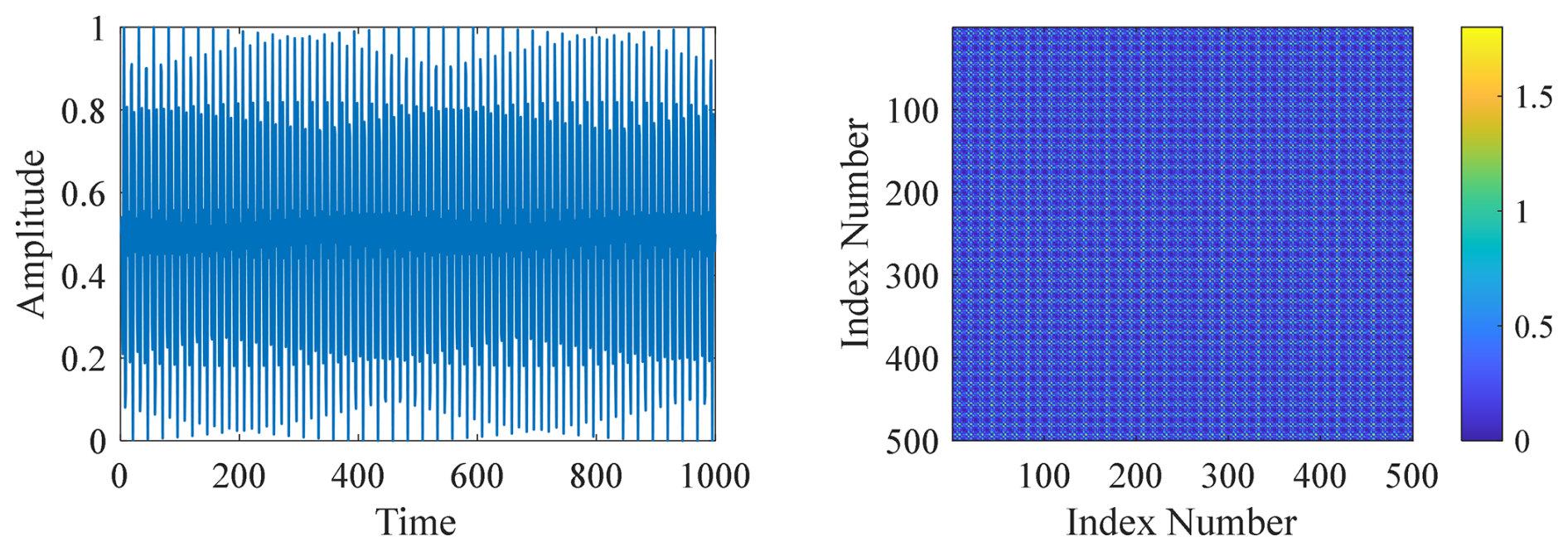
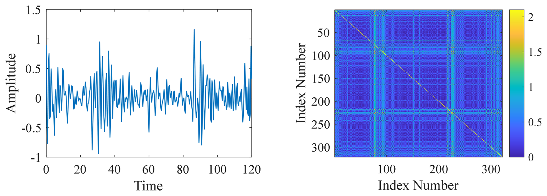
Figure 2 Defect signal with its recurrence plot (left: defect signal; right: recurrence plot).

2.2 Recurrence quantification analysis

The nonlinear and non-smooth characteristics of rolling-bearing defect signals make the traditional defect feature extraction methods based on the smoothness of the signals limited, while the recurrence quantification analysis (RQA) method is an effective method that can quantify the recurrence phenomenon of the system shown in the recurrence diagrams on the basis of improving the recurrence diagrams (Zbilut and Webber, 2006). Recurrence quantification analysis is an effective method to quantify the recurrence phenomenon in recurrence diagrams. The recurrence diagram is a qualitative means of analyzing the complexity of a signal, while the RQA method is a quantitative method derived from the recurrence diagram. The nonlinear characteristics of the RQA method include the following: recurrence rate (RR), recurrence entropy (ENTR), layered rate (LAM), determination rate (DET), recurrence number (TT), and average diagonal length (L). The recurrence rate, recurrence entropy, and average diagonal length (L) of the recurrence diagram are the most important characteristics of the recurrence diagram. Further more, out of the above characteristics, recursion rate, recursion entropy, and recursion trend are the more commonly used measures.

Recurrence rate (RR) refers to the ratio of the number of points appearing in the recurrence plot to the number of points appearing in the complete distance matrix (Yu et al., 2025). The RR counts only the black points in the recurrence map and is a measure used to evaluate the density of recurrence points, representing the frequency of recurrence of phase points and the degree of clustering of trajectories in phase space.

$$\begin{array}{}\text{(1)}& \mathrm{RR}={\displaystyle \frac{\mathrm{1}}{M^{\mathrm{2}}}}{\mathrm{\Sigma }}_{i,j=\mathrm{1}}^M{\mathbf{R}}_{ij}\end{array}$$

In the above, R_ij denotes the recurrence matrix, and M is the number of points on the horizontal or vertical axis in the recurrence plot.

Recursive entropy (ENTR) refers to the distribution of the length of diagonal structures in a recursive graph. It is a metric that can be used to measure the strength of the periodicity of a recursive graph.

$$\begin{array}{}\text{(2)}& \mathrm{ENTR}=-{\mathrm{\Sigma }}_{l=l_{min}}^{M}p\left(l\right)\ln \left(pl\right)\end{array}$$

In the above, p(l) represents the number of line segments of length l that are parallel to the main diagonal.

Recurrence trend (TREND) refers to the degree of the speed of change in the rate of recurrence as the main diagonal on the recurrence graph transitions to the other two corners, essentially reflecting the degree of mixing and non-stationarity of the signal.

$$\begin{array}{}\text{(3)}& \mathrm{TREND}={\displaystyle \frac{{\sum }_{\mathit{\tau }=\mathrm{1}}^{\stackrel{\mathrm{̃}}{N}}\left(\mathit{\tau }-\frac{\stackrel{\mathrm{̃}}{N}}{\mathrm{2}}\right)\left({\mathrm{RR}}_{\mathit{\tau }}-〈{\mathrm{RR}}_{\mathit{\tau }}〉\right)}{{\sum }_{\mathit{\tau }=\mathrm{1}}^{\stackrel{\mathrm{̃}}{N}}{\left(\mathit{\tau }-\frac{\stackrel{\mathrm{̃}}{N}}{\mathrm{2}}\right)}^{\mathrm{2}}}}\end{array}$$

Here, 〈RR_τ〉 denotes the size of the mean of the time series, and RR_τ denotes the rate of recurrence of the different parts of the time series after averaging over $\stackrel{\mathrm{̃}}{N}$. If the time measure changes in the sliding window, the size of the recurrence trend depends mainly on the size of the window, and so, for different sizes of the window, the resulting recurrence trend may be very different.

2.3 Data dynamic network

The correlation coefficient is an important indicator of the size of statistical relationships and the strength of relationships between different data. Data dynamic network characteristics refer to the artificially established network of connections among data, which can effectively strengthen the defect characteristics of the data set. By studying the instantaneous linear relationship between adjacent signals, based on the Pearson correlation coefficient in conjunction with the sliding time window, we can arrange the defect data into a time-dependent network, completing the analysis of the two metrics of correlation and phase synchronization and thus endowing the data with useful dynamic attributes (Vinck et al., 2011).

The overall correlation coefficient between two variables X and Y is defined as follows:

$$\begin{array}{}\text{(4)}& {\mathit{\rho }}_{X,Y}={\displaystyle \frac{\mathrm{cov}(X,Y)}{{\mathit{\sigma }}_X{\mathit{\sigma }}_Y}}={\displaystyle \frac{E\left[\left(X-{\mathit{\mu }}_X\right)\left(Y-{\mathit{\mu }}_Y\right)\right]}{{\mathit{\sigma }}_X{\mathit{\sigma }}_Y}},\end{array}$$

where σ_X and σ_Y denote the corresponding standard deviations.

The Pearson correlation coefficient r is expressed as follows:

$$\begin{array}{}\text{(5)}& r={\displaystyle \frac{\sum _{i=\mathrm{1}}^n\left(X_i-\stackrel{\mathrm{‾}}{X}\right)\left(Y_i-\stackrel{\mathrm{‾}}{Y}\right)}{\sqrt{\sum _{i=\mathrm{1}}^n{\left(X_i-\stackrel{\mathrm{‾}}{X}\right)}^{\mathrm{2}}}\sqrt{\sum _{i=\mathrm{1}}^n{\left(Y_i-\stackrel{\mathrm{‾}}{Y}\right)}^{\mathrm{2}}}}}.\end{array}$$

For network connectivity, in the analysis of specific signals, phase synchronization is an important indication of the interaction between different nodes (Onias and Viol, 2013).

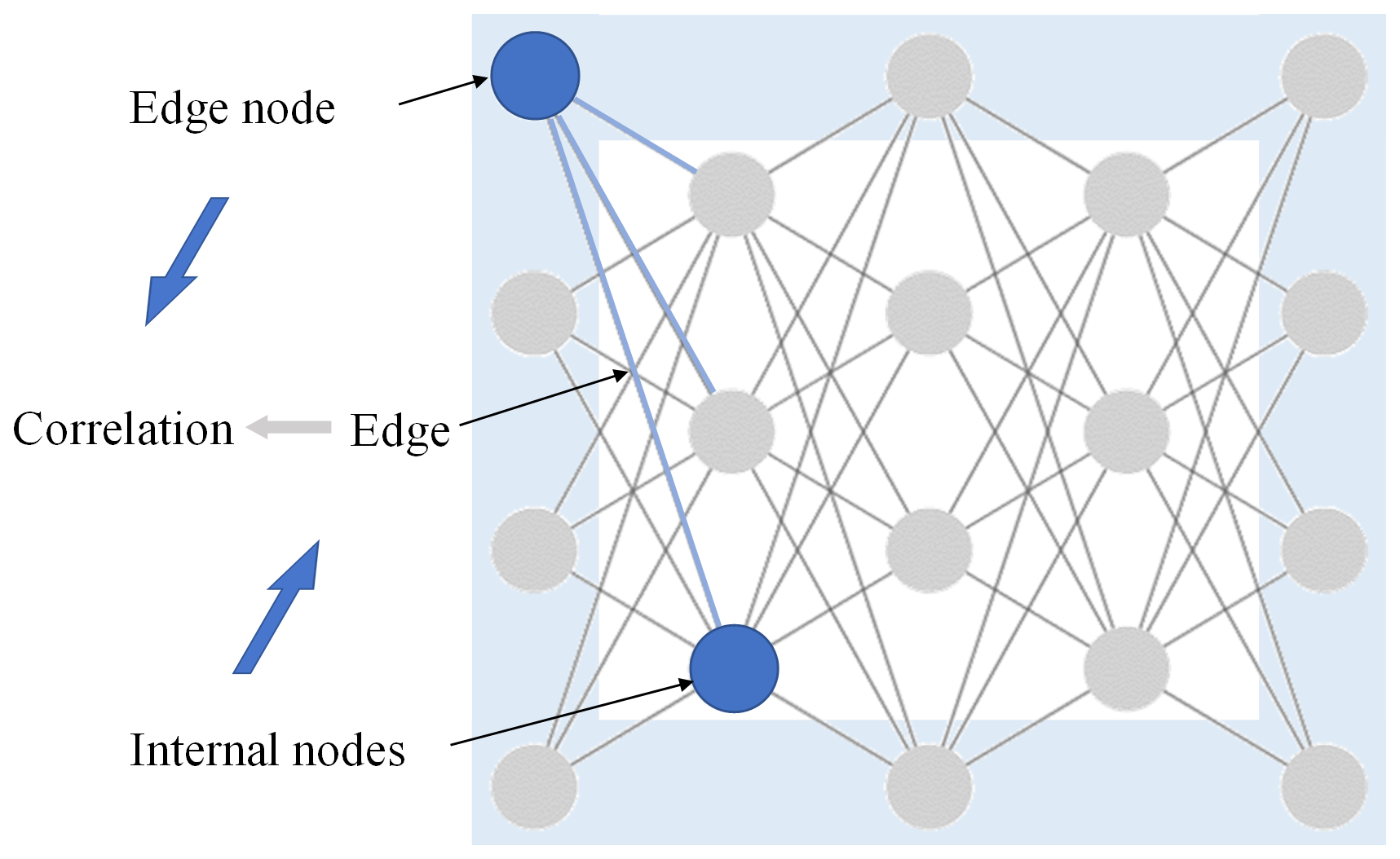
If two signal sequences are phase synchronized then the correlation between the nodes represented by these two signals is stronger. As shown in the Fig. 3, data dynamic network characteristics refer to the dynamic functional network matrix composed of different nodes and connected edges between nodes, with the connected edges reflecting the correlation and consistency between the nodes, thus enabling us to show the dynamic changes in the defects in specific parts of the rolling bearing.

Figure 3 Example of a network connection.

2.4 Data sets

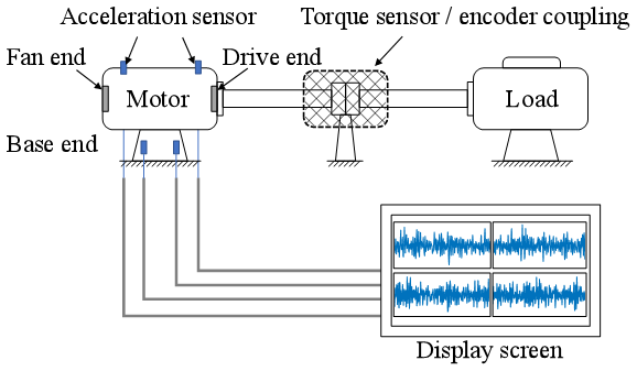
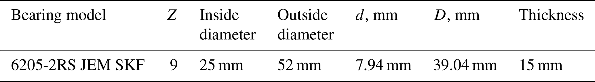
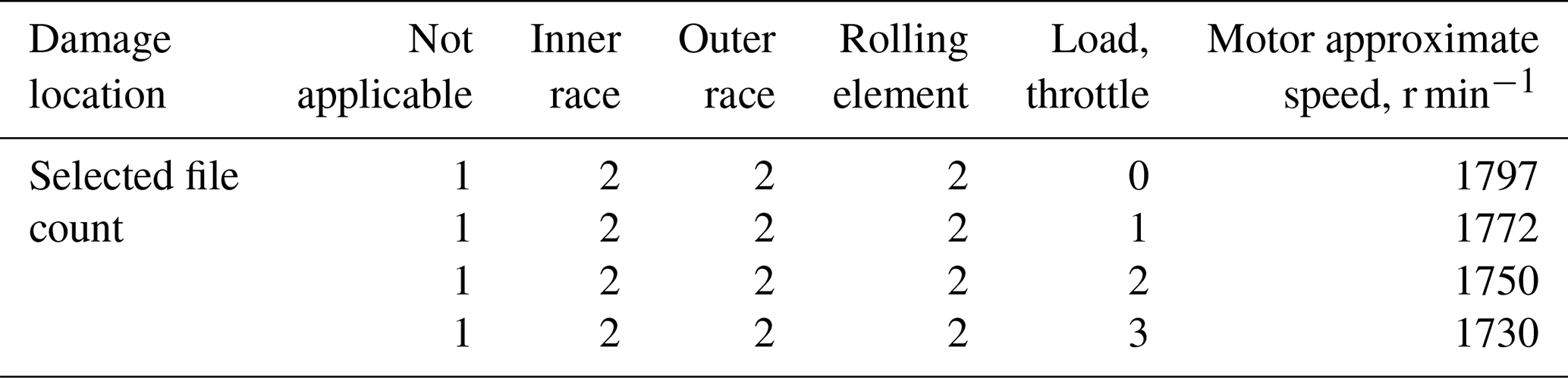
The data set used in this paper is the publicly available rolling-bearing failure data set from Case Western Reserve University (CWRU) (21). The entire experimental platform consists of a 1.5 kW motor, torque transducer, power meter, etc., as shown in Fig. 4. The data used in this paper are the drive end bearing data; the bearing is sealed on both sides and is manufactured by SKF, with deep groove ball bearings (model 6205). The experimental sampling frequency is 12 kHz, and the specific parameters are shown in Table 1. There are three types of defects detected in the experimental bearings, namely, inner-ring defects, outer-ring defects, and rolling-element defects. Together with the normal data, there are four final experimental data types selected. In this paper, for the inner-ring failure, outer-ring failure, and rolling-body failure, we selected eight relevant data files, with four data files being selected for normal data for subsequent defect extraction and training tests; the specific types are shown in Table 2.

Figure 4 Bearing failure experiment.

Table 1 Bearing models and parameters.

Table 2 Data selected for this paper.

3 Experimental verification

3.1 Data set enhancement

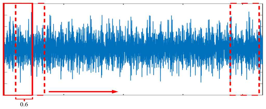
This paper is based on the programming for each selected data file, applying the written algorithm for the sliding-time-window slicing process to enhance the data set; the repetition rate is 0.6 for a total of 100 slides to complete the initial processing of the data, as shown in Fig. 5.

Figure 5 Demonstration of sliding time window.

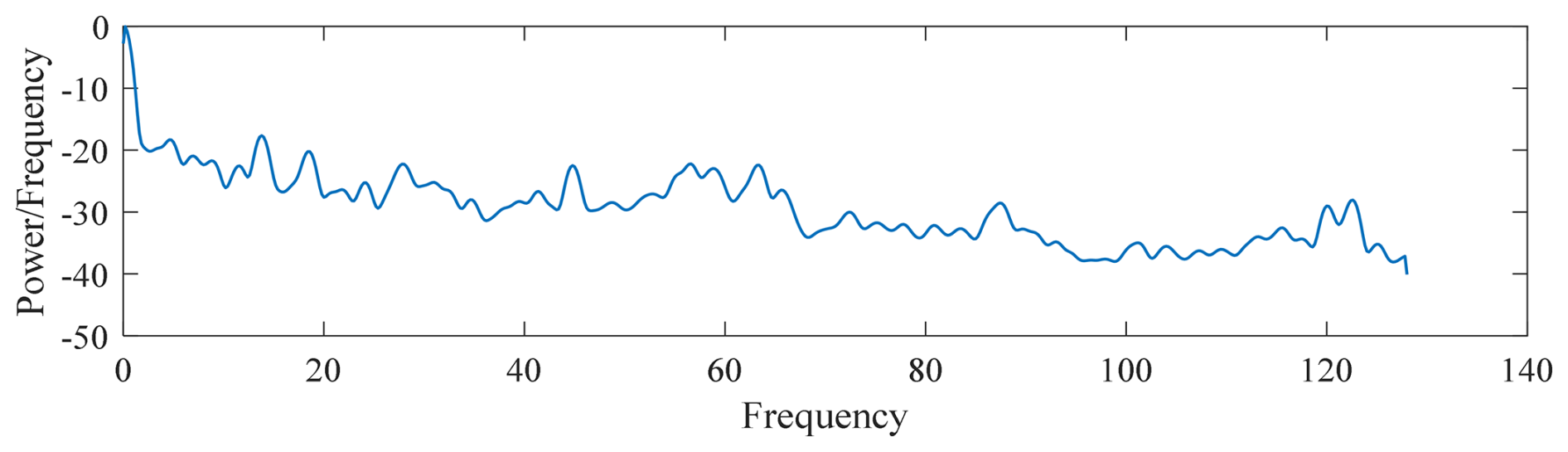
3.2 Power spectral density analysis

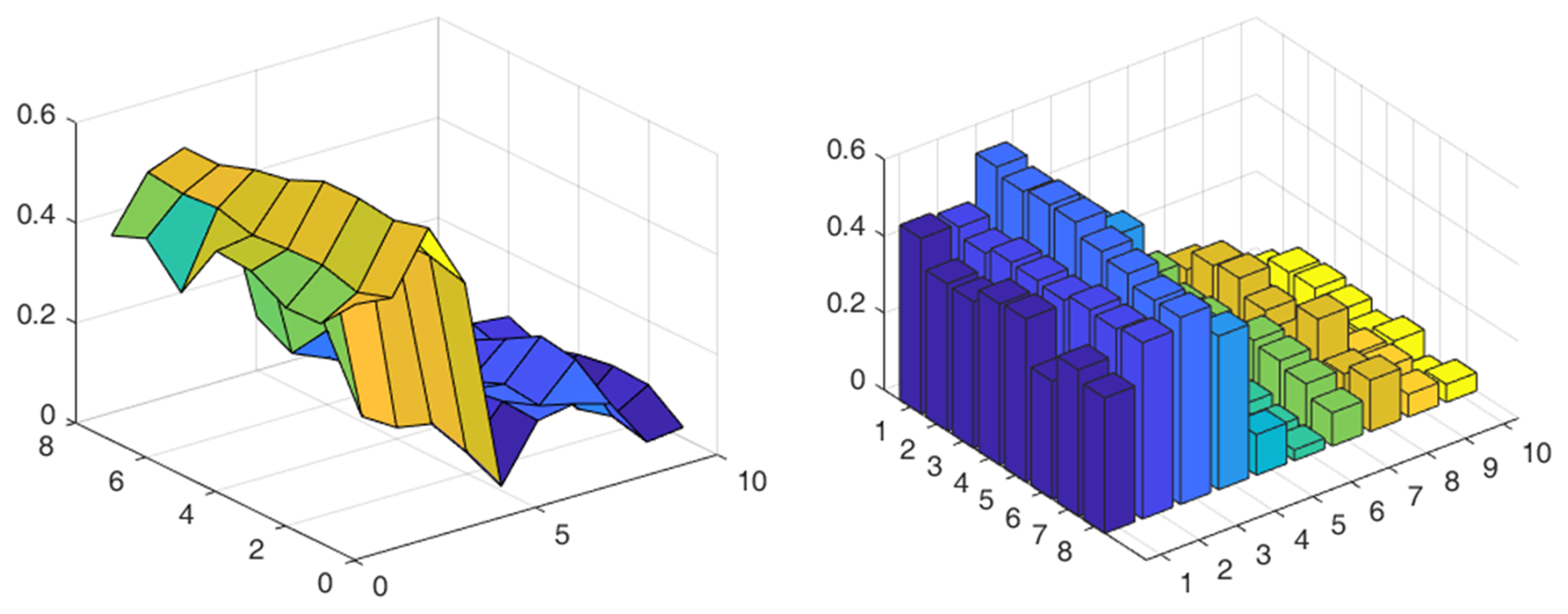
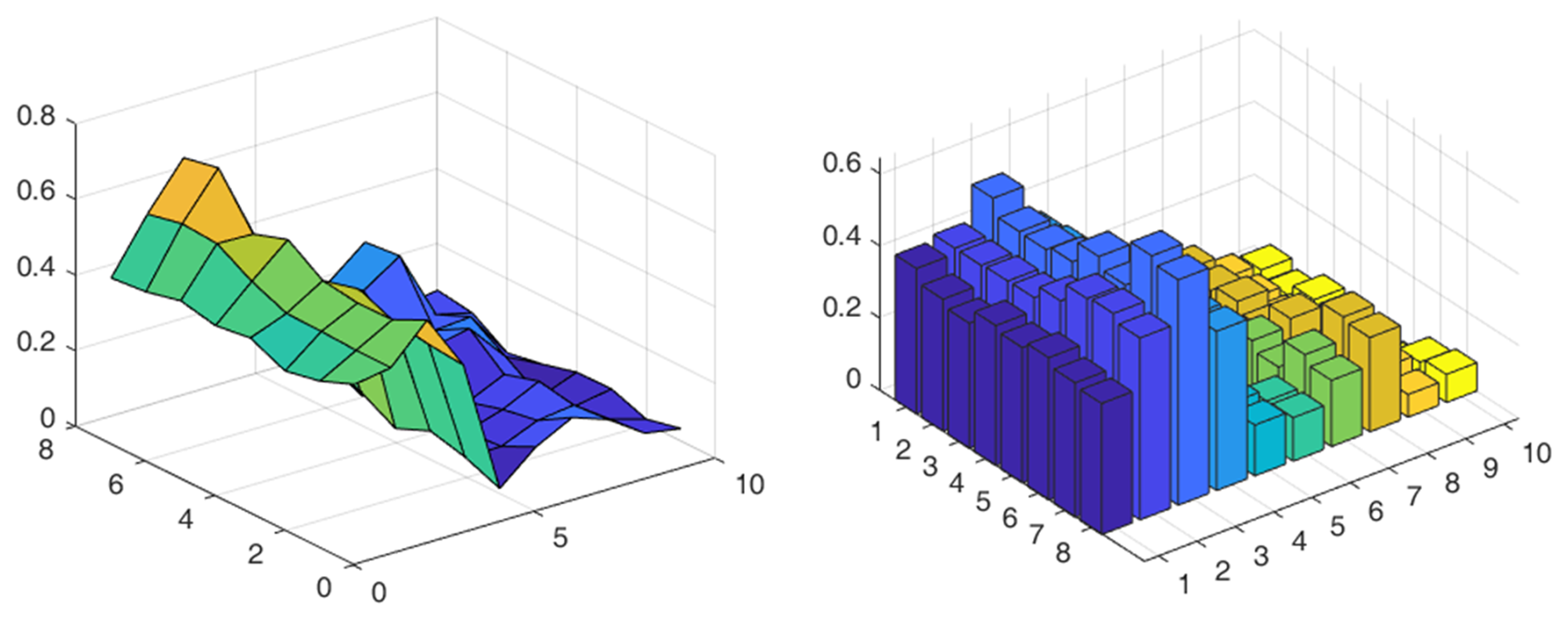
The data obtained from the power spectral density analysis of the filtered processed data in this section can be used as part of the feature quantity for subsequent machine learning, with the power spectral density being shown in Figs. 6 to 9.

Figure 6 Power spectrum of the inner-ring-defect sample.

Figure 7 Power spectrum of the outer-ring-defect sample.

Figure 8 Power spectrum of rolling-body-failure samples.

Figure 9 Power spectrum of a normal sample.

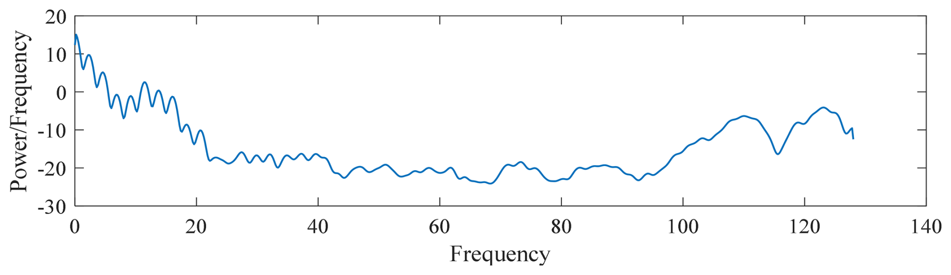
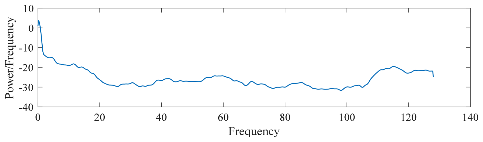
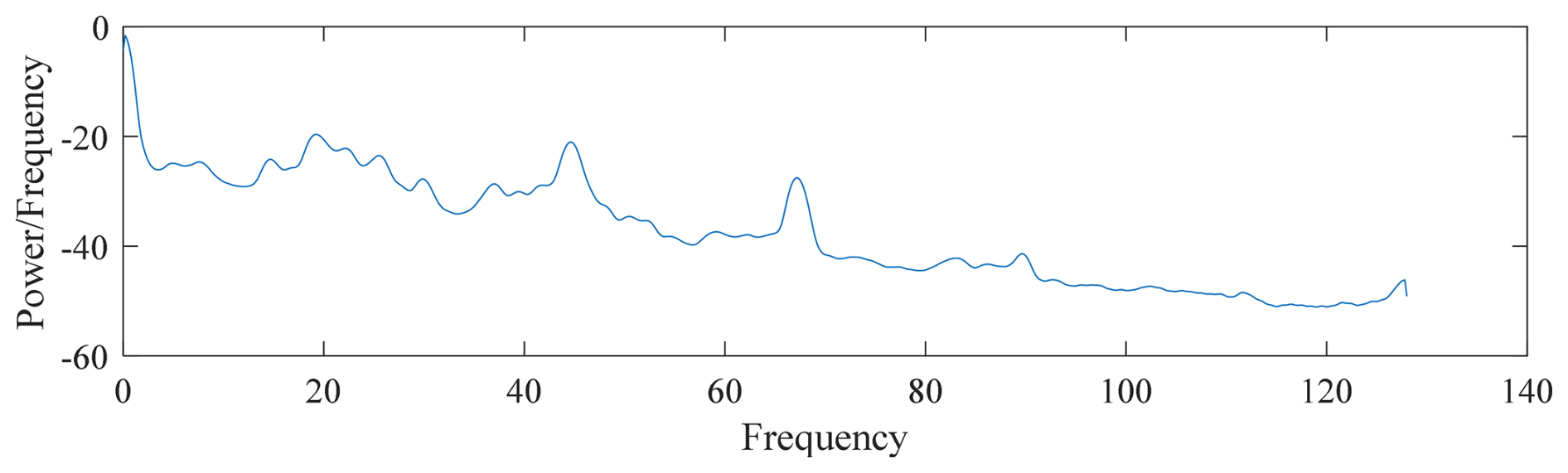
The power spectral density visualization is shown in Figs. 10 to 12. After visualization, the power spectral density analysis of different defect areas can intuitively show the magnitude of and difference in energy in different frequency ranges, which can be used as the input features of the subsequent convolutional neural network with good results.

Figure 10 Visualization of power spectral density of inner-ring defects.

Figure 11 Visualization of power spectral density of outer-ring defects.

Figure 12 Visualization of power spectral density of rolling-body defects.

3.3 Recursive-feature extraction

Using the recurrence map and the RQA method for quantitative analysis, each file of the obtained features is 8 rows × 11 columns, in which the first 10 columns represent the power spectral densities in different frequency ranges, and these features can comprehensively reflect the dynamic characteristics and complexity of the data series. The new 11th column is the recurrence rate, which provides important information about the phase space reconstruction in the data and provides strong support for the subsequent data interpretation and model construction. The inner-circle-defect sample (no. 1) with the new recurrence rate is shown in Table 3.

Table 3 Sample inner-circle failures with new recurrence rates. PSD: power spectral density.

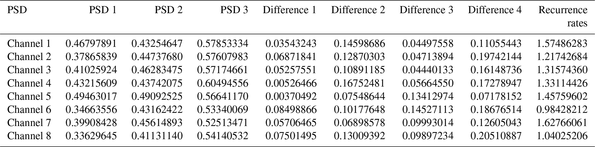
The extracted features are visualized and processed as shown in Fig. 13.

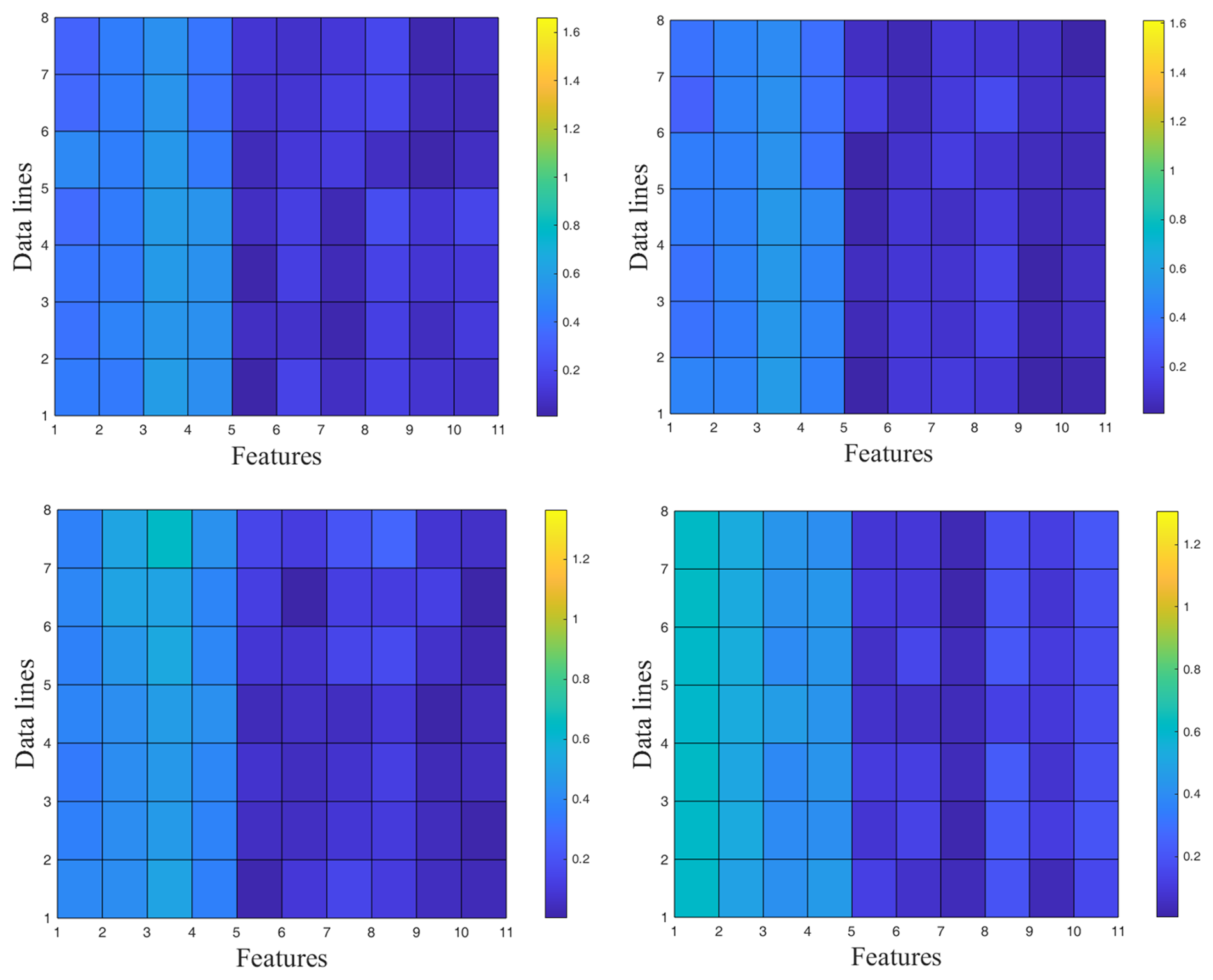
Figure 13 Data recursive-feature visualization (first row: inner and outer ring; second row: roller and normal).

3.4 Data dynamic network feature extraction

A new defect data set is obtained by applying data set enhancement techniques such as sliding-time-window slicing. Within this data set, there are eight groups of data for each different defect type; each group consists of 100 rows of data after filtering and amplitude–frequency analysis using the Pearson correlation coefficient analysis method mentioned in the above section, with subsequent calculation of the correlation coefficients of the data in two adjacent rows so as to generate the strengthened feature matrix and conversion of the data into an 8 × 10 network matrix with time window processing so as to obtain the dynamic. The dynamic network matrix is constructed based on the sliding-time-window method as shown in Fig. 14.

Figure 14 Constructing dynamic networks based on a sliding-time-window approach.

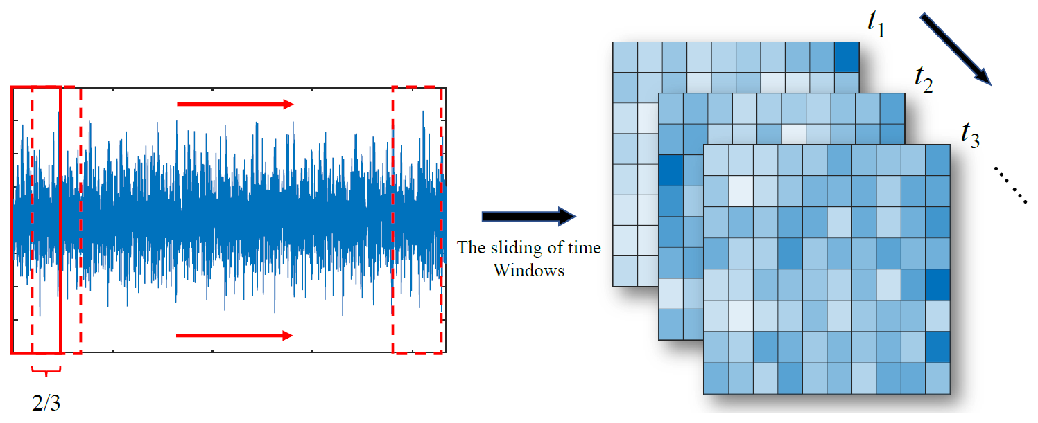
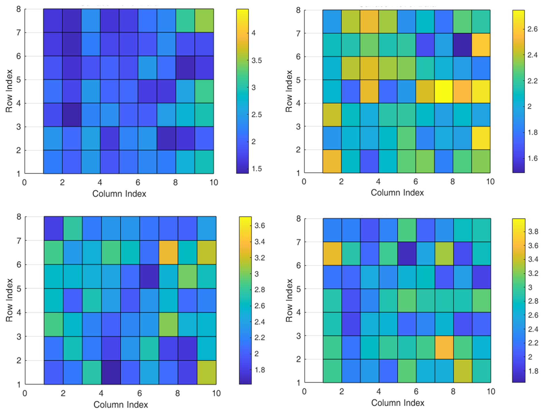
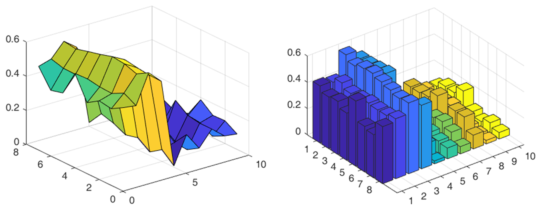
Figure 15 Visualization of dynamic network features of data (first row: inner and outer ring; second row: roller and normal).

The extracted features are visualized and processed as shown in Fig. 15, from which it can be intuitively seen that the dynamic network features are more effective in feature visualization than energy feature analysis due to their dynamic properties. Through the comparison between different colors, the difference between dynamic network features extracted from different samples can be clearly seen.

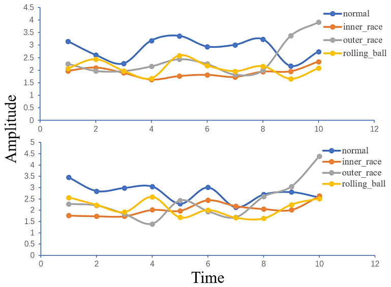
The variation in the strength of the constructed network nodes over time is shown in Fig. 16, from which it can be concluded that there are some fluctuations in the strength of the nodes of each defect type over time, with relatively large fluctuations in the outer-ring defects.

Figure 16 Plot of average strength of network nodes over time.

3.5 Convolutional neural network architecture

Convolutional neural networks (CNNs) have become a key data-processing tool in the defect identification research of mechanical equipment (Zhu, 2024). The purpose of this section is to analyze and study the practical application effect of the convolutional neural network model based on energy features, recursive features, and dynamic network features in bearing defect identification. This chapter will introduce the specific structure of the convolutional neural network and the construction process in detail, including the convolutional layer, nonlinear activation function, pooling operation, fully connected layer, and other major parts, and will also clarify their functions and interconnections and then introduce the forward-propagation algorithm; the back-propagation algorithm; and a series of evaluation indexes, including the accuracy rate, the loss function, and the confusion matrix, in order to conduct a further, reasonable evaluation for different models. The experimental results show that, compared with the different models, the algorithms are more accurate and more efficient.

The experimental results show that, compared with the convolutional neural network (CNN) model using only energy features, the model with new data recursive features and the model using data dynamic features have certain dynamic attributes due to their association with time; additionally, the convergence speed and diagnostic accuracy have been improved, which indicates that the data recursive features and the dynamic network features can effectively enhance the model's ability to recognize the defect signals, thus validating the robustness of this paper's method. Thus, the advantages of the method in this paper in terms of robustness and generalizability are verified.

3.5.1 The pooling layer

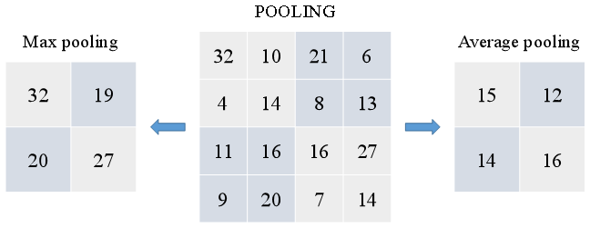
The pooling layer is a method to reduce the complexity of the model (LeCun et al., 2015). By reducing the resolution of the feature map, the parameters of the neural network can be effectively reduced, and, at the same time, the adaptability to the input data in displacement and scale changes is enhanced. In practice, there are two common pooling methods: maximum pooling and mean pooling, as shown in Fig. 17.

Figure 17 Example of pooling operation.

3.5.2 Full-connectivity layer

A fully connected layer is one of the components of a classifier, which is characterized by the fact that every neuron in the current layer is connected to all neurons in the previous layer. While operations such as convolutional, pooling, and activation layers map the original data to the hidden feature space, the fully connected layer serves to map the resulting “distributed feature representation” to the sample labeling space. The equation is as follows:

$$\begin{array}{}\text{(6)}& x_{k+\mathrm{1}}=\mathrm{\Sigma }{W}_k{x}_k+b_{k+\mathrm{1}},\end{array}$$

where x_k+1 denotes the current neuron output result, W_k denotes the connection weight, and b_k represents the size of the bias value.

3.6 Forward-propagation algorithm and back-propagation algorithm

The forward-propagation algorithm is the basis of convolutional neural network prediction, which can be calculated layer by layer until the final result is output according to the hierarchical structure of the network. The back-propagation algorithm is one of the key cores of the convolutional neural network training; through the calculation of the gradient of the loss function relative to the parameters of each layer, it can realize the updating of the network parameters and, ultimately, can achieve the purpose of minimizing the difference between the prediction results and the real value.

3.6.1 Forward-propagation algorithm

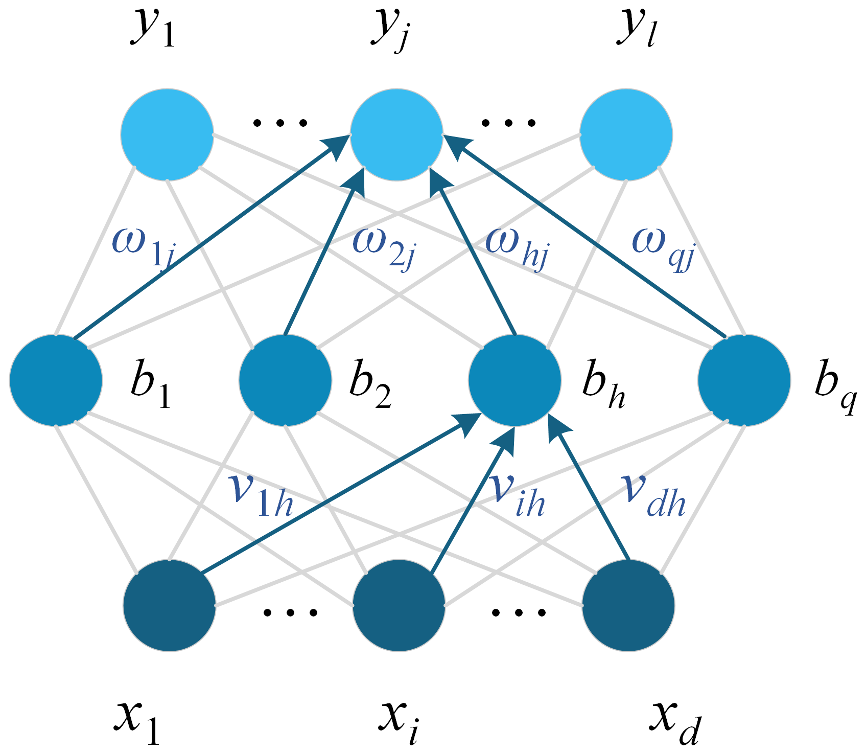
The forward-propagation algorithm is one of the common processes used to perform neural network operations. The information is transmitted layer by layer by combining with weights and biases to finally obtain the output, where the activity state of each layer is determined by the corresponding activation function of that layer, as shown in Fig. 18. After completing the output, the forward propagation will quantitatively analyze the error size according to some evaluation metrics. The specific calculations are as follows:

$$\begin{array}{}\text{(7)}& a_j^l=\mathit{\sigma }\left(\sum _k{\mathit{\omega }}_{jk}^l{a}_k^{l-\mathrm{1}}+b_j^l\right).\end{array}$$

The matrix is of the form

$$\begin{array}{}\text{(8)}& a^l=\mathit{\sigma }\left(w^l{a}^{l-\mathrm{1}}+b^l\right).\end{array}$$

Here, $b_j^l$ denotes the bias value of the neuron j in the layer l, $a_j^l$ denotes the activation value of the neuron j in the layer l, and w denotes the weights of two neurons in two adjacent layers.

Figure 18 Forward-propagation demonstration.

3.6.2 Back-propagation algorithm

The back-propagation algorithm (Zhou, 2016), also known as the BP algorithm, addresses the need for an error back-propagation operation, as shown in Fig. 19.

Figure 19 Symbolic representation in back-propagation networks and algorithms.

For a training example (x_k,y_k), we use the following equation:

$$\begin{array}{}\text{(9)}& {\widehat{y}}_j^k=f({\mathit{\beta }}_j-{\mathit{\theta }}_j).\end{array}$$

The input into the hidden-layer neuron h is calculated as follows:

$$\begin{array}{}\text{(10)}& {\mathit{\alpha }}_h=\sum _{i=\mathrm{1}}^d{\mathit{\nu }}_{ih}{x}_i.\end{array}$$

The input into the output neuron j is calculated as follows:

$$\begin{array}{}\text{(11)}& {\mathit{\beta }}_j=\sum _{h=\mathrm{1}}^q{\mathit{\omega }}_{h_j}{b}_h.\end{array}$$

The mean squared error is calculated as follows:

$$\begin{array}{}\text{(12)}& E_k={\displaystyle \frac{\mathrm{1}}{\mathrm{2}}}\sum _{j=\mathrm{1}}^l{\left({\widehat{y}}_j^k-y_j^k\right)}^{\mathrm{2}}.\end{array}$$

Given the error E_k, assuming a learning rate η, the weight updates are computed as follows:

$$\begin{array}{}\text{(13)}& \mathrm{\Delta }{w}_{hj}=-\mathit{\eta }{\displaystyle \frac{\partial E_k}{\partial {\mathit{\omega }}_{hj}}}.\end{array}$$

Using the chain rule, we can compute the partial derivatives:

$$\begin{array}{}\text{(14)}& {\displaystyle \frac{\partial E_k}{\partial {\mathit{\omega }}_{h_j}}}={\displaystyle \frac{\partial E_k}{\partial {\widehat{y}}_j^k}}\cdot {\displaystyle \frac{\partial {\widehat{y}}_j^k}{\partial {\mathit{\beta }}_j}}\cdot {\displaystyle \frac{\partial {\mathit{\beta }}_j}{\partial w_{hj}}}.\end{array}$$

Let

$$\begin{array}{}\text{(15)}& g_j=-{\displaystyle \frac{\partial E_k}{\partial {\widehat{y}}_j^k}}\cdot {\displaystyle \frac{\partial {\widehat{y}}_j^k}{\partial {\mathit{\beta }}_j}}={\widehat{y}}_j^k(\mathrm{1}-{\widehat{y}}_j^k)(y_j^k-{\widehat{y}}_j^k).\end{array}$$

Then

$$\begin{array}{}\text{(16)}& \mathrm{\Delta }{w}_{hj}=-\mathit{\eta }{\displaystyle \frac{\partial E_k}{\partial \mathit{\omega }{n}_j}}=\mathit{\eta }{g}_j{b}_h.\end{array}$$

Similarly,

$$\begin{array}{}\text{(17)}& \mathrm{\Delta }{\mathit{\theta }}_j=-\mathit{\eta }{g}_j.\end{array}$$

3.7 Assessment of indicators

Performance metrics are a measure of how much generalizability a model has. During convolutional neural network training, evaluation metrics such as loss function, accuracy, confusion matrix, and receiver operating characteristic (ROC) curve are commonly used to evaluate the model for the next step of testing and optimization (Zhou, 2016). Through these evaluation metrics, we can quantitatively assess the robustness and generalization capabilities of the model, specifically its ability to maintain consistent performance when confronted with new test data.

3.7.1 Loss function

Loss refers to the difference between the predicted value and the true value when applying machine learning. There are two main types of loss functions commonly used in the task of performing classification: the cross-entropy loss (CEL) and the mean squared error (MSE).

Figure 20 Curves of loss and accuracy (left: loss; right: accuracy).

The cross-entropy loss is calculated as follows:

$$\begin{array}{}\text{(18)}& L={\displaystyle \frac{\mathrm{1}}{n}}\sum _{i=\mathrm{1}}^n\left(-\sum _{j=\mathrm{1}}^c{y}_i\log p_i\right),\end{array}$$

where n represents the training batch size, C represents the number of classes, y represents the sample labeling distribution, and p represents the model prediction distribution.

The mean square error loss is calculated as follows:

$$\begin{array}{}\text{(19)}& \mathrm{MSE}={\displaystyle \frac{{\sum }_{i=\mathrm{1}}^n{\left(y_i-y_j^p\right)}^{\mathrm{2}}}{n}}.\end{array}$$

3.7.2 Accuracy

Precision reflects the accuracy of the model created for prediction. Accuracy and error rate are opposite concepts of each other: the higher the accuracy, the better the performance of the designed model is proved. The specific accuracy and error rate are calculated as outlined below.

• Accuracy.

  $$\begin{array}{}\text{(20)}& \mathrm{acc}={\displaystyle \frac{\mathrm{1}}{m}}\sum _{i=\mathrm{1}}^m\prod \left(f\left(x_i\right)=y_i\right).\end{array}$$

  In the above, y_i denotes the true label corresponding to the ith sample in the test set, and f(x_i) denotes its predicted label.

• Error rate.

  $$\begin{array}{}\text{(21)}& E={\displaystyle \frac{\mathrm{1}}{m}}\sum _{i=\mathrm{1}}^m\prod \left(f\left(x_i\right)\ne y_i\right)=\mathrm{1}-\mathrm{acc}.\end{array}$$

3.7.3 Confusion matrix

The confusion matrix can visualize the quality of machine learning model evaluation and thus determine how well the model performs. An example of the confusion matrix is shown in Table 4.

Table 4 Confusion matrix example.

3.8 Data dynamic network characterization

Since the ReLU function is constant at 0 in the negative half-axis of the coordinate axis, the derivative is also constant at 0, resulting in the disappearance of the gradient in this region, a property known as unilateral suppression, which helps the model to learn a more efficient feature representation. Since the ReLU function has very good properties, this function is used as the activation function in the construction of the convolutional neural network in this chapter.

Table 5 Structure parameters of the convolutional neural network model based on data energy characteristics.

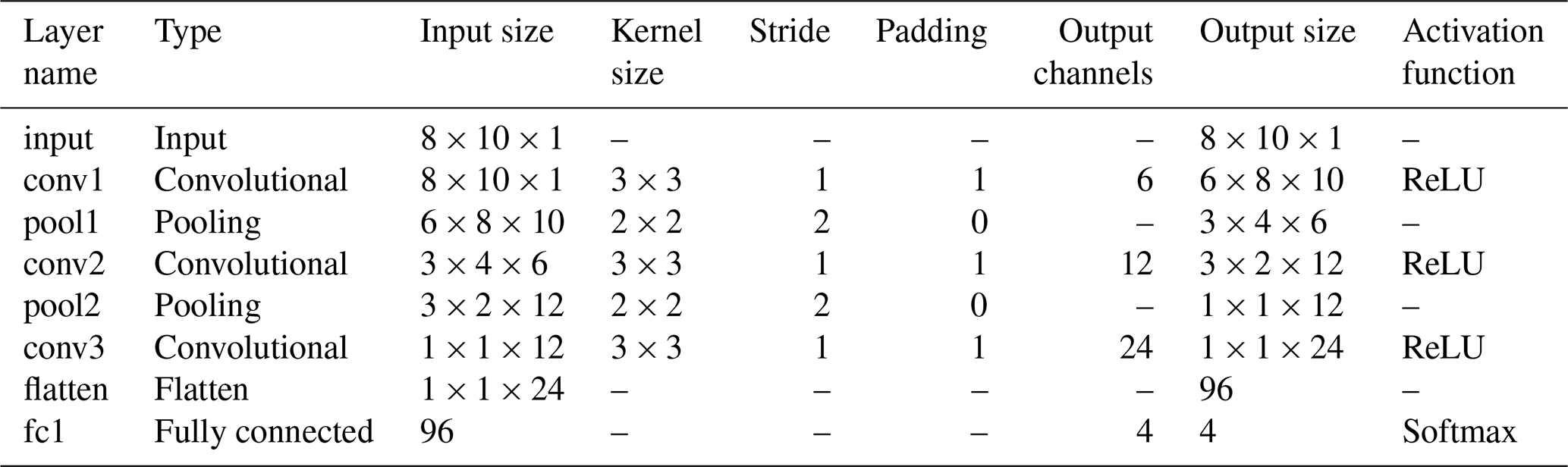
The structural parameters of the convolutional neural network model based on energy analysis are shown in Table 5.

3.9 Synthesis based on dynamic network characterization of data

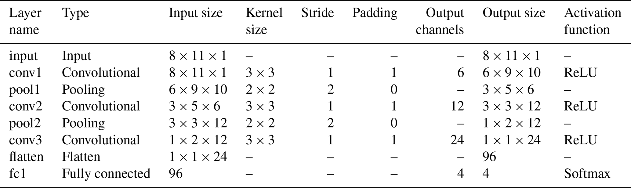
The structural parameters of the convolutional neural network model based on the dynamic network characteristics of the data are shown in Table 6.

Table 6 Structure parameters of the convolutional neural network model based on data dynamic network characterization.

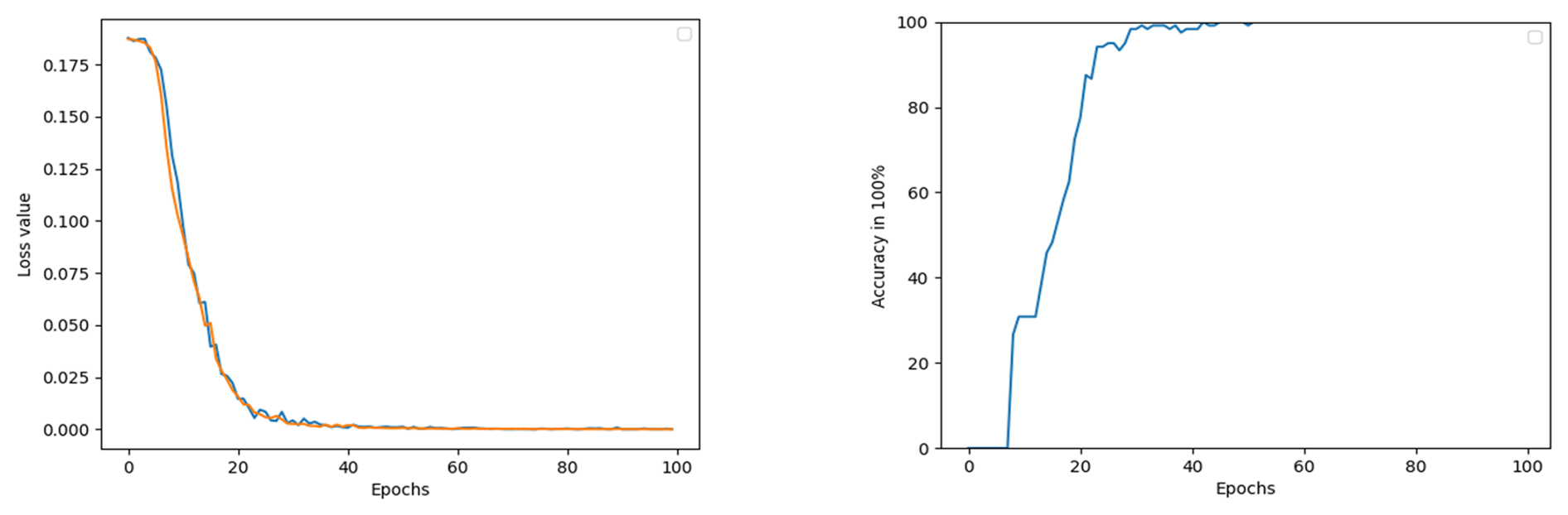
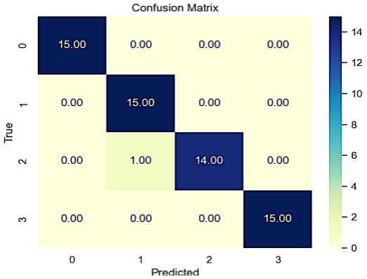
In the input into the convolutional neural network, the loss, accuracy, and confusion matrix obtained after 100 epochs of testing are depicted in Figs. 20 and 21. In Fig. 20a, the blue line represents the loss curve during training, and the orange line represents the loss curve during testing.

Figure 21 Confusion matrix.

Figure 22 Confusion matrix generated for the new test set.

As the iteration time increases, the loss value decreases sharply. When the epochs reach 20, the loss value gets to around 1 %, and the good match of the loss curves for training and testing validates the good accuracy of the proposed methods and procedures for bearing defect identification. In Fig. 20b, the accuracy curve during iteration is provided. The accuracy is 95 % an epoch of 30 and 98 % at an epoch of 40. Around 100 % accuracy is obtained at epoch of 52. The significance of the proposed methods and procedures for bearing defect identification can be clearly proved and observed. The obtained results serve as a good proof of concept for the practical bearing defect identification and can be implemented in actual mechanical engineering.

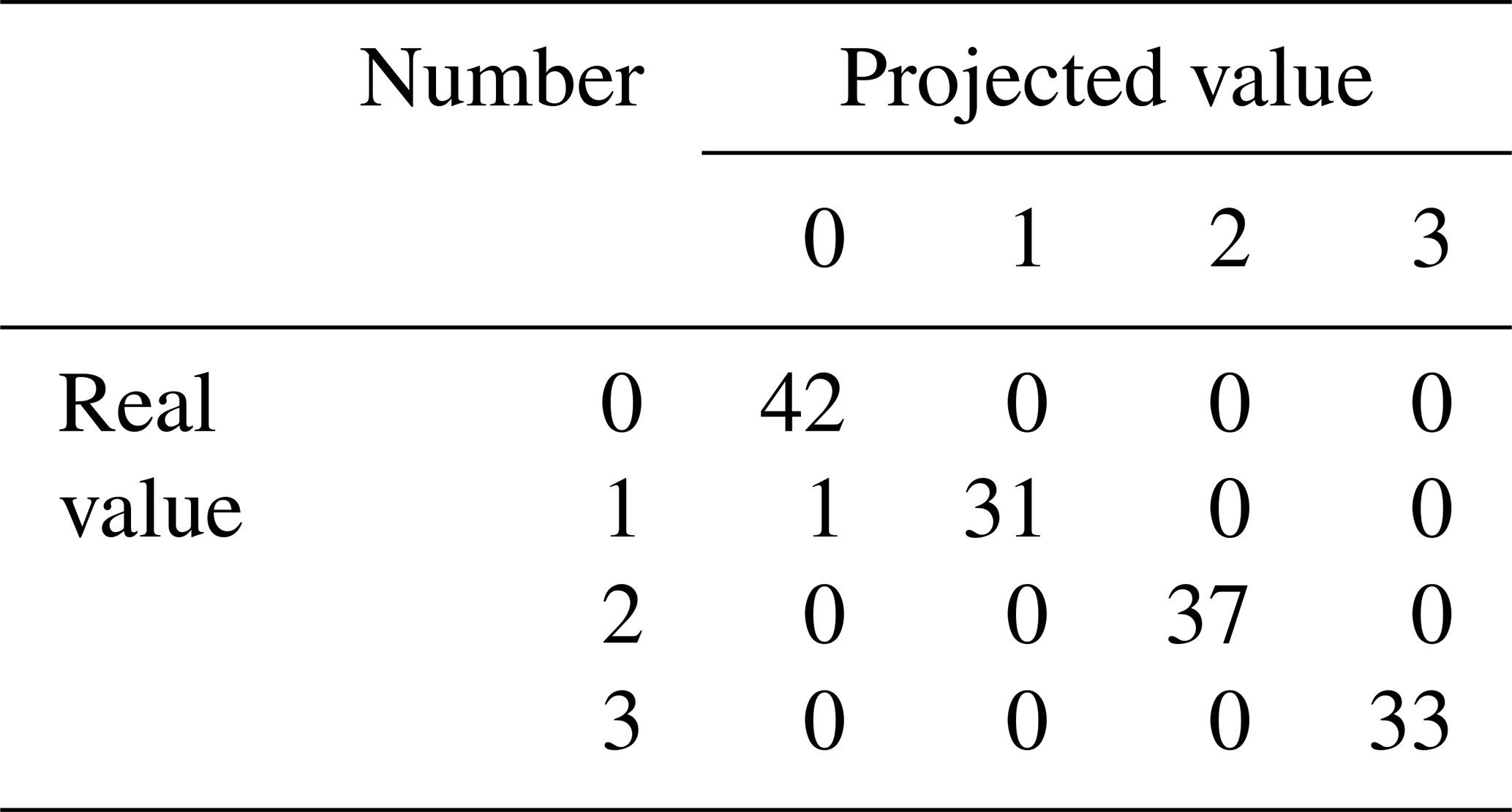
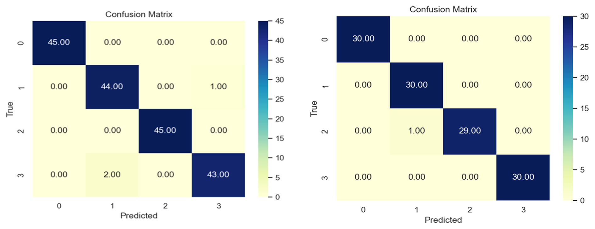
The confusion matrix obtained from a new test set is depicted in Fig. 22. In the confusion matrixes shown in Figs. 21 and 22, the horizontal axis represents the predicted value; the vertical axis represents the true value; and labels 0, 1, 2, and 3, respectively, represent four defect types: normal, inner-ring defect, outer-ring defect, and rolling-element defect. In Fig. 22a, out of 180 test samples, 177 were accurately predicted, achieving an accuracy of 98.333 %. In Fig. 22b, 119 out of 120 test samples were correctly identified, resulting in an accuracy of 99.167 %. These high accuracy rates indicate that the model performs exceptionally well and can be reliably used in real-world bearing defect identification to precisely identify various types of bearing defects.

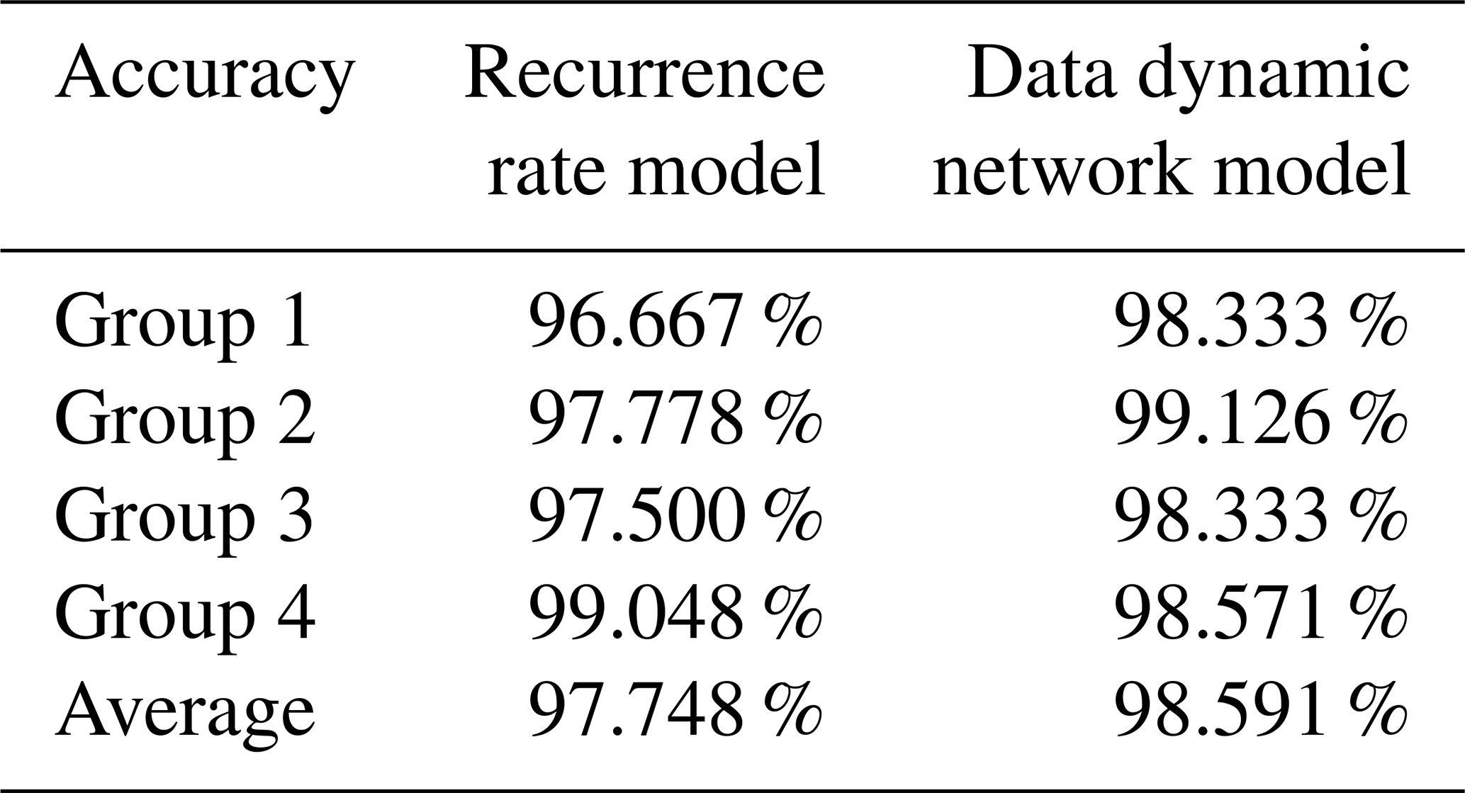
3.10 Model comparison

A comparison of model performance between the two feature extraction methods is presented in Table 7. The convolutional neural network model utilizing recurrence features achieved an average accuracy of 97.748 %. In contrast, the model employing dynamic network features attained a significantly higher average accuracy of 98.591 %. These findings indicate that the dynamic network, capturing the inherent dynamics of the system, provides an optimal feature representation. This offers a superior data preprocessing strategy for practical bearing fault diagnosis applications.

Table 7 Comparison of two models.

4 Conclusions

In this study, we performed an effective bearing defect detection using the proposed feature enhancements of data dynamic networks. The research is summarized as follows.

In this paper, we proposed a data dynamic network for data enhancement for bearing defect identifications. Nodes and edges of data are constructed for the establishment of a data dynamic network. Together with the feature fusion techniques, the energy, recurrence rates, and amplitude–frequency spectrums are reconstructed in the time-delayed phase space for preparation of bearing defect identification. The accuracy of bearing defect identification reaches up to 98.5 %.

A convolutional neural network (CNN) model based on data recursive features and dynamic network features is designed. The effectiveness in bearing defect identification is verified through experiments. The generalizability and robustness of the intelligent neural network are improved. A more effective defect detection algorithm is explored.

The preliminary results of this paper contribute new ideas to the field of bearing defect identification. We hope that the paper can provide inspiration and promote the development of intelligent defect identifications of bearing defects.