Integrating elite opposition-based learning and Cauchy–Gaussian mutation into sparrow search algorithm for time–impact collaborative trajectory optimization of robotic manipulators

Aiming at the problems such as low convergence efficiency, local optimization traps, and insufficient multi-objective cooperative optimization existing in the multi-objective trajectory planning of industrial robotic arms, this study proposes a trajectory optimization method based on a new improved sparrow search algorithm (NISSA). Firstly, by integrating elite reverse learning and the Cauchy–Gaussian mutation strategy, the NISSA algorithm is constructed to enhance the global search ability and convergence efficiency. Secondly, the 3–5–3 polynomial interpolation method is adopted to establish a continuous and smooth joint spatial trajectory model to ensure the continuity of position, velocity, and acceleration. Finally, a multi-objective optimization function integrating time and mechanical shock is constructed, and the collaborative optimization of efficiency and stability is achieved through dynamic weight allocation. The simulation experiments based on the IRB4600 six-axis robotic arm show that compared with the traditional sparrow algorithm (SSA) and multi-strategy improved particle swarm optimization (MIPSO), NISSA shortens the trajectory planning time by 19.6 %, reduces path redundancy by 25.7 %, increases the iterative convergence speed by 68.75 %, and reduces the standard deviation of joint acceleration to 28.5 % of the original value. The research results provide theoretical support and technical implementation paths for the high-precision and efficient operation of robotic arms in complex industrial scenarios.

1 Introduction

Traditional path planning methods can be divided into two categories: analytic algorithms based on geometric constraints and probabilistic algorithms based on random sampling. Among them, the former, such as the artificial potential field method and unit decomposition method, relies on accurate environment modeling, and its algorithm complexity increases exponentially with the number of obstacles, which has the defects of high computational complexity and insufficient real-time performance. Although the latter algorithms, such as rapidly expanding random tree (Dai et al., 2022) and probabilistic road map (Gasparetto et al., 2015), can effectively solve the search problem in high-dimensional space, they are prone to local optimal solution convergence in dynamic obstacle scenarios, and the path smoothness is difficult to guarantee.

In the field of industrial automation, robot motion planning is a core enabling technology for intelligent manufacturing systems. Its key scientific issue lies in establishing an optimal motion trajectory generation mechanism that meets multiple constraints. As a crucial component of robotic arm control, trajectory planning aims to construct an optimal motion path integrating efficiency, precision, and safety within the operational workspace. This process plays a decisive role in ensuring the smooth execution of preset trajectories. Scientifically designed trajectory planning can not only improve the production efficiency of robotic arms but also reduce system energy consumption and mechanical wear, which is of great significance for promoting the development of industrial automation towards intelligence. The current mainstream algorithm systems can be divided into four categories: probability-complete algorithms based on random sampling (Yuan et al., 2021; Cornell and Hung, 2018), local planning algorithms based on potential field theory (Xu et al., 2022; Chen et al., 2023), global planning algorithms based on topological mapping (e.g., probabilistic roadmap (PRM); Chen et al., 2021; Bansal and Anand, 2024), and intelligent decision-making algorithms based on deep reinforcement learning (Tang et al., 2022; Sekkat et al., 2021).

To address the inherent drawbacks and issues of traditional potential field algorithms, such as being prone to falling into local minima, failure to reach the target, poor dynamic obstacle avoidance capability, and problems related to safety and efficiency, Xia et al. (2023) proposed an improved velocity potential field (IVPF) algorithm, which incorporates the direction factor, obstacle velocity factor, and tangential velocity factor. When encountering dynamic obstacles, the IVPF algorithm can better avoid obstacles and ensure the safety of both humans and robotic arms. Lumelsky (1987) proposed a non-heuristic algorithm that can generate reasonable (though not optimal) collision-free paths. In this method, paths are continuously (dynamically) planned based on the current position of the manipulator and sensory feedback. A suitable objective function is formulated by integrating the requirements of time optimality and path smoothness. To tackle the problems of blind expansion and low efficiency in the rapidly exploring random tree (RRT) algorithm and its improved variants, Chai and Wang (2022) proposed a greedy sampling space reduction strategy which reduces redundant expansion of random trees by dynamically adjusting the sampling space. Additionally, a novel narrow passage judgment method is developed based on the environment surrounding sampling points. Cao et al. (1996) utilized trigonometric functions to evaluate the connection between paths and obstacles in space and identified collision-free paths in three-dimensional space. Subsequently, through sampling space partitioning, obstacle discretization, and a distance weight function, Cao proposed a method to adaptively adjust the node sampling probability of the RRT algorithm in space, aiming to reduce unnecessary sampling nodes and optimize sampling efficiency.

However, the aforementioned methods still face numerous challenges in practical applications, such as long planning time, high computational resource consumption, insufficient real-time performance, frequent failure to obtain globally optimal paths, poor path smoothness, risks of planning failure in complex scenarios, and high algorithm complexity.

To address this critical technical challenge, researchers worldwide have proposed innovative solutions. Ekrem and Aksoy (2023) developed a hybrid trajectory planning method combining particle swarm optimization (PSO) and quintic polynomial interpolation. By constructing continuous joint-space trajectories with continuity in position, velocity, and acceleration, this method achieves accurate Cartesian space coordinate transformation through forward kinematics analysis and ultimately realizes time optimization via the shortest path search.

Meanwhile, Jia et al. (2024) adopted dynamic time warping (DTW) to align the time of multiple demonstration examples and extracted ideal trajectory features using the Gaussian mixture model (GMM) and Gaussian mixture regression (GMR). Their improved dynamic movement primitives (DMP) framework enables effective trajectory parameter learning and motion generalization. Miao et al. (2022) proposed a hybrid strategy combining a genetic algorithm with an enhanced particle swarm optimization algorithm and demonstrated the effect of trajectory optimization through simulation experiments. Kaljaca et al. (2020) innovatively formulated a custom objective function in the joint space and realized optimal node traversal scheduling through a time interpolation algorithm under motion constraints. Zhang et al. (2023) introduced deep reinforcement learning into trajectory planning for 6-degree-of-freedom (6-DOF) robotic arms and designed a multi-objective optimization framework to synergistically optimize key indicators, including trajectory accuracy, energy efficiency, and motion smoothness. Jiang et al. (2023) improved the artificial potential field method by integrating the rapidly exploring random tree (RRT) algorithm, which effectively addressed the local minimum problem in obstacle avoidance paths for bending robots while enhancing path smoothness and path length optimization performance. Dai et al. (2020) fused the gravitational search algorithm with the ant colony algorithm; through the design of hierarchical search strategies and heuristic functions, they significantly improved the convergence speed and global optimization capability of path planning for spatial truss robots. Sun et al. (2025) proposed a fusion method combining modified adaptive particle swarm optimization (MAPSO) and fuzzy PD control. This method not only optimized the trajectory of flexible arms using 3–5–3 hybrid polynomials but also substantially reduced driving torque and vibration interference, providing a new paradigm for the precision control of flexible structures.

In existing literature, analytical algorithms rely on accurate modeling but have high complexity and insufficient real-time performance; probabilistic algorithms are prone to local optimality and poor path smoothness; and improved algorithms, though improved, still have limitations. To address issues such as low convergence efficiency, susceptibility to local optimization traps, and insufficient multi-objective collaborative optimization in multi-objective trajectory planning of industrial robotic arms, this study proposes a trajectory optimization method based on the novel improved sparrow search algorithm (NISSA). The algorithm integrates elite reverse learning and the Cauchy–Gaussian mutation strategy to enhance global search capability and convergence efficiency. It adopts the 3–5–3 polynomial interpolation to establish a continuous and smooth joint-space trajectory model, ensuring continuity of position, velocity, and acceleration. A multi-objective optimization function integrating time and mechanical shock is constructed, achieving collaborative optimization of efficiency and stability through dynamic weight allocation. Simulation experiments based on the IRB4600 six-axis robotic arm verify the superiority of this method.

2 Problem description

2.1 Establishment of the kinematic model

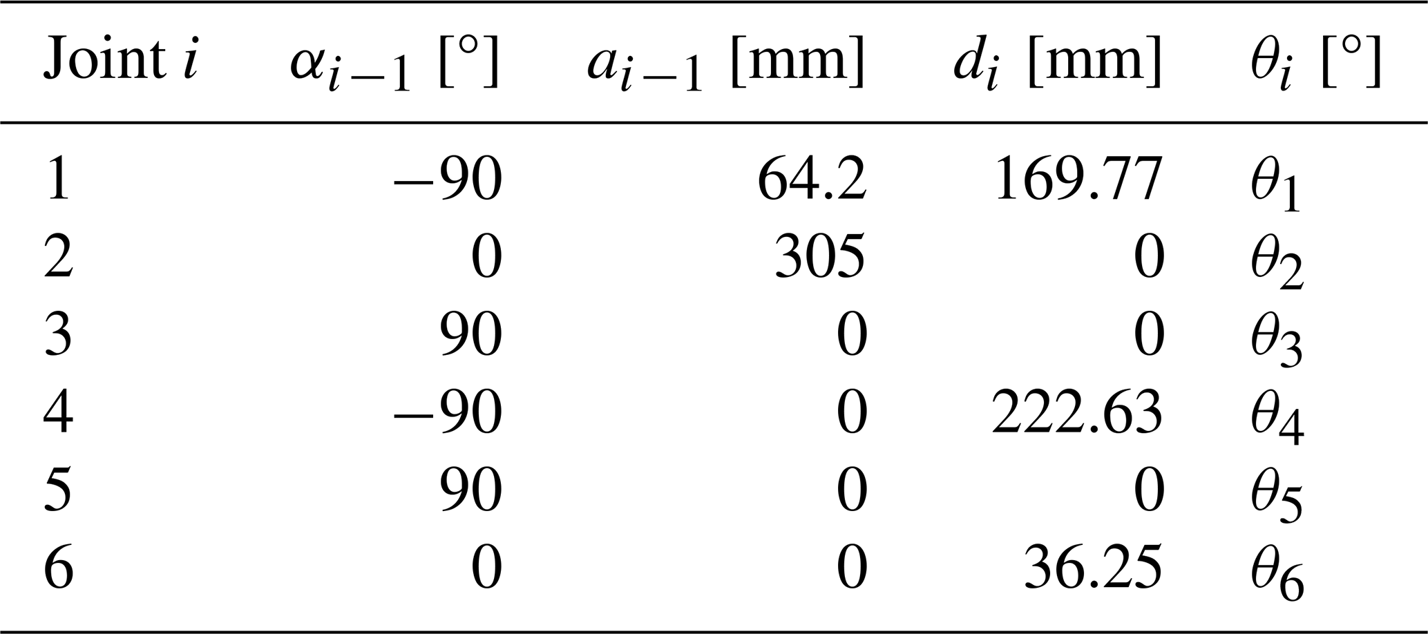
In this study, the AR4 robotic arm was taken as the experimental object. Aiming at the structural characteristics of its series connecting rods, the Denavit–Hartenberg (D–H) parameter method was adopted to establish the kinematic model of the robotic arm. As shown in Fig. 1, the coordinate systems of the connecting rods of each joint were constructed based on the standard D–H modeling rule system. The corresponding D–H parameters are detailed in Table 1. The parameter table contains four basic parameters: the torsion angle of the connecting rod α_i; the length of the connecting rod a_i; the joint rotation angle θ_i; and the deflection of the connecting rod d_i, which completely characterizes the spatial transformation relationship between adjacent coordinate systems.

Figure 1 D–H model.

Table 1 D–H parameters of the robotic arm.

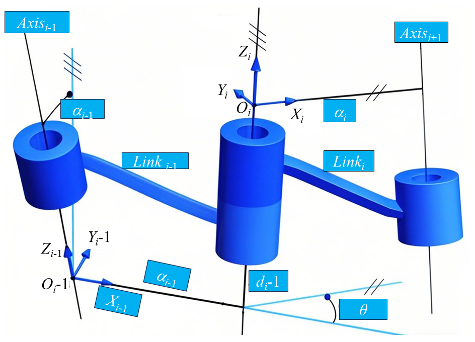
In the coordinate system shown in Fig. 2, the pose transformation between the coordinate system i of the adjacent robotic arm and i−1 is composed of two rotations and two translation operations, and its homogeneous transformation matrix is constructed through the above transformation process.

$$\begin{array}{}\text{(1)}& \begin{array}{rl}& {}_i^{i-\mathrm{1}}T=\\ & \left[\begin{array}{cccc}\cos {\mathit{\theta }}_i& -\sin {\mathit{\theta }}_i& \mathrm{0}& a_{i-\mathrm{1}}\\ \sin {\mathit{\theta }}_i\cos {\mathit{\alpha }}_{i-\mathrm{1}}& \cos {\mathit{\theta }}_i\cos {\mathit{\alpha }}_{i-\mathrm{1}}& -\sin {\mathit{\alpha }}_{i-\mathrm{1}}& -d_i\sin {\mathit{\alpha }}_{i-\mathrm{1}}\\ \sin {\mathit{\theta }}_i\sin {\mathit{\alpha }}_{i-\mathrm{1}}& \cos {\mathit{\theta }}_i\sin {\mathit{\alpha }}_{i-\mathrm{1}}& \cos {\mathit{\alpha }}_{i-\mathrm{1}}& d_i\cos {\mathit{\alpha }}_{i-\mathrm{1}}\\ \mathrm{0}& \mathrm{0}& \mathrm{0}& \mathrm{1}\end{array}\right]\end{array}\end{array}$$

Figure 2 Connecting rod coordinate system.

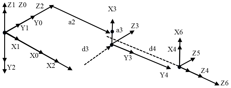
Substitute the D–H parameters in Table 1 into Eq. (1) to construct the transformation matrices of each joint coordinate system. Through the product operation of continuous matrices, the pose transformation matrix of the end effector is derived. This matrix represents the pose information of the end effector relative to the base coordinate system.

$$\begin{array}{}\text{(2)}& {}_{\mathrm{6}}^{\mathrm{0}}T{=}_{\mathrm{1}}^{\mathrm{0}}{T}_{\mathrm{2}}^{\mathrm{1}}{T}_{\mathrm{3}}^{\mathrm{2}}{T}_{\mathrm{4}}^{\mathrm{3}}{T}_{\mathrm{5}}^{\mathrm{4}}{T}_{\mathrm{6}}^{\mathrm{5}}T=\left[\begin{array}{cccc}{n}_x& o_x& a_x& p_x\\ n_y& o_y& a_y& p_y\\ n_z& o_z& a_z& p_z\\ \mathrm{0}& \mathrm{0}& \mathrm{0}& \mathrm{1}\end{array}\right]\end{array}$$

2.2 Trajectory planning is carried out by polynomial interpolation method

To ensure the continuity of the position, velocity, and acceleration of the trajectory, this study adopted the 3–5–3 polynomial interpolation method (Wang et al., 2020a) to optimize the trajectory of the robotic arm, reduce the vibration during the movement, protect the mechanical structure of the robotic arm, and improve the accuracy of the operation. Select four path points, x_i1, x_i2, x_i3, and x_i4. The three time periods formed by adjacent two points can be expressed as 0–t₁, t₁–t₂, and t₂–t₃.

The functional relationship between the displacement of the ith joint and time t is expressed as

$$\begin{array}{}\text{(3)}& \left\{\begin{array}{l}{\mathit{\theta }}_{i\mathrm{1}}\left(t\right)=a_{i\mathrm{13}}{t}_{\mathrm{1}}^{\mathrm{3}}+a_{i\mathrm{12}}{t}_{\mathrm{1}}^{\mathrm{2}}+a_{i\mathrm{11}}{t}_{\mathrm{1}}+a_{i\mathrm{10}},\\ {\mathit{\theta }}_{i\mathrm{2}}\left(t\right)=a_{i\mathrm{25}}{t}_{\mathrm{2}}^{\mathrm{5}}+a_{i\mathrm{24}}{t}_{\mathrm{2}}^{\mathrm{4}}+a_{i\mathrm{23}}{t}_{\mathrm{2}}^{\mathrm{3}}+a_{i\mathrm{22}}{t}_{\mathrm{2}}^{\mathrm{2}}+a_{i\mathrm{21}}{t}_{\mathrm{2}}+a_{i\mathrm{20}},\\ {\mathit{\theta }}_{i\mathrm{3}}\left(t\right)=a_{i\mathrm{33}}{t}_{\mathrm{3}}^{\mathrm{3}}+a_{i\mathrm{32}}{t}_{\mathrm{3}}^{\mathrm{2}}+a_{i\mathrm{31}}{t}_{\mathrm{3}}+a_{i\mathrm{30}}.\end{array}\right.\end{array}$$

By taking the first derivative, the functional expression of the velocity and time of the ith joint can be obtained:

$$\begin{array}{}\text{(4)}& \left\{\begin{array}{l}{\mathit{\theta }}_{i\mathrm{1}}\left(t\right)=\mathrm{3}{a}_{i\mathrm{13}}{t}_{\mathrm{1}}^{\mathrm{2}}+\mathrm{2}{a}_{i\mathrm{12}}{t}_{\mathrm{1}}+a_{i\mathrm{11}},\\ {\mathit{\theta }}_{i\mathrm{2}}\left(t\right)=\mathrm{5}{a}_{i\mathrm{25}}{t}_{\mathrm{2}}^{\mathrm{4}}+\mathrm{4}{a}_{i\mathrm{24}}{t}_{\mathrm{2}}^{\mathrm{3}}+\mathrm{3}{a}_{i\mathrm{23}}{t}_{\mathrm{2}}^{\mathrm{2}}+\mathrm{2}{a}_{i\mathrm{22}}{t}_{\mathrm{2}}+a_{i\mathrm{21}},\\ {\mathit{\theta }}_{i\mathrm{3}}\left(t\right)=\mathrm{3}{a}_{i\mathrm{33}}{t}_{\mathrm{3}}^{\mathrm{2}}+\mathrm{2}{a}_{i\mathrm{32}}{t}_{\mathrm{3}}+a_{i\mathrm{31}}.\end{array}\right.\end{array}$$

Then, calculate the second derivative to obtain the functional relationship between the acceleration of the ith joint and time:

$$\begin{array}{}\text{(5)}& \left\{\begin{array}{l}{\mathit{\theta }}_{i\mathrm{1}}\left(t\right)=\mathrm{6}{a}_{i\mathrm{13}}{t}_{\mathrm{1}}+\mathrm{2}{a}_{i\mathrm{12}}{t}_{\mathrm{1}},\\ {\mathit{\theta }}_{i\mathrm{2}}\left(t\right)=\mathrm{20}{a}_{i\mathrm{25}}{t}_{\mathrm{2}}^{\mathrm{3}}+\mathrm{12}{a}_{i\mathrm{24}}{t}_{\mathrm{2}}^{\mathrm{2}}+\mathrm{6}{a}_{i\mathrm{23}}{t}_{\mathrm{2}}+\mathrm{2}{a}_{i\mathrm{22}},\\ {\mathit{\theta }}_{i\mathrm{3}}\left(t\right)=\mathrm{6}{a}_{i\mathrm{33}}{t}_{\mathrm{3}}+\mathrm{2}{a}_{i\mathrm{32}}{t}_{\mathrm{3}}.\end{array}\right.\end{array}$$

The angular velocity and angular acceleration of the robotic arm joint at the start and end of motion are both zero, and they should be equal when passing through the intermediate position. The time-dependent transformation matrix can be expressed as

$$\begin{array}{}\text{(6)}& \begin{array}{rl}& A=\\ & \left[\begin{array}{ccccccccccccccc}{t}_{\mathrm{1}}^{\mathrm{3}}& t_{\mathrm{1}}^{\mathrm{2}}& t_{\mathrm{1}}& \mathrm{0}& \mathrm{0}& \mathrm{0}& \mathrm{0}& \mathrm{0}& -\mathrm{1}& \mathrm{0}& \mathrm{0}& \mathrm{0}& \mathrm{0}& \mathrm{0}& \mathrm{0}\\ \mathrm{3}{t}_{\mathrm{1}}^{\mathrm{2}}& \mathrm{2}{t}_{\mathrm{1}}& \mathrm{1}& \mathrm{0}& \mathrm{0}& \mathrm{0}& \mathrm{0}& -\mathrm{1}& \mathrm{0}& \mathrm{0}& \mathrm{0}& \mathrm{0}& \mathrm{0}& \mathrm{0}& \mathrm{0}\\ \mathrm{6}{t}_{\mathrm{1}}& \mathrm{2}& \mathrm{0}& \mathrm{0}& \mathrm{0}& \mathrm{0}& -\mathrm{2}& \mathrm{0}& \mathrm{0}& \mathrm{0}& \mathrm{0}& \mathrm{0}& \mathrm{0}& \mathrm{0}& \mathrm{0}\\ \mathrm{6}{t}_{\mathrm{1}}& \mathrm{2}& \mathrm{0}& \mathrm{0}& \mathrm{0}& \mathrm{0}& -\mathrm{2}& \mathrm{0}& \mathrm{0}& \mathrm{0}& \mathrm{0}& \mathrm{0}& \mathrm{0}& \mathrm{0}& -\mathrm{1}\\ \mathrm{0}& \mathrm{0}& \mathrm{0}& t_{\mathrm{2}}^{\mathrm{3}}& t_{\mathrm{2}}& t_{\mathrm{2}}^{\mathrm{4}}& t_{\mathrm{2}}^{\mathrm{3}}& t_{\mathrm{2}}^{\mathrm{2}}& t_{\mathrm{2}}& \mathrm{0}& \mathrm{0}& \mathrm{0}& \mathrm{0}& -\mathrm{1}& \mathrm{0}\\ \mathrm{0}& \mathrm{0}& \mathrm{0}& \mathrm{5}{t}_{\mathrm{2}}^{\mathrm{4}}& \mathrm{4}{t}_{\mathrm{2}}^{\mathrm{3}}& \mathrm{3}{t}_{\mathrm{2}}^{\mathrm{2}}& \mathrm{2}{t}_{\mathrm{2}}& \mathrm{1}& \mathrm{0}& \mathrm{0}& \mathrm{0}& \mathrm{0}& -\mathrm{4}& \mathrm{0}& \mathrm{0}\\ \mathrm{0}& \mathrm{0}& \mathrm{0}& \mathrm{20}{t}_{\mathrm{2}}^{\mathrm{3}}& \mathrm{12}{t}_{\mathrm{2}}^{\mathrm{2}}& \mathrm{6}{t}_{\mathrm{2}}& \mathrm{2}& \mathrm{0}& \mathrm{0}& \mathrm{0}& \mathrm{0}& -\mathrm{2}& \mathrm{0}& \mathrm{0}& \mathrm{0}\\ \mathrm{0}& \mathrm{0}& \mathrm{0}& \mathrm{0}& \mathrm{0}& \mathrm{0}& \mathrm{0}& \mathrm{0}& \mathrm{0}& \mathrm{0}& \mathrm{0}& t_{\mathrm{3}}^{\mathrm{2}}& t_{\mathrm{3}}^{\mathrm{2}}& t_{\mathrm{3}}& \mathrm{1}\\ \mathrm{0}& \mathrm{0}& \mathrm{0}& \mathrm{0}& \mathrm{0}& \mathrm{0}& \mathrm{0}& \mathrm{0}& \mathrm{0}& \mathrm{0}& \mathrm{0}& \mathrm{3}{t}_{\mathrm{3}}^{\mathrm{2}}& \mathrm{2}{t}_{\mathrm{3}}^{\mathrm{1}}& \mathrm{1}& \mathrm{0}\\ \mathrm{0}& \mathrm{0}& \mathrm{0}& \mathrm{0}& \mathrm{0}& \mathrm{0}& \mathrm{0}& \mathrm{0}& \mathrm{0}& \mathrm{0}& \mathrm{0}& \mathrm{6}{t}_{\mathrm{3}}& \mathrm{2}& \mathrm{0}& \mathrm{0}\\ \mathrm{0}& \mathrm{0}& \mathrm{0}& \mathrm{1}& \mathrm{0}& \mathrm{0}& \mathrm{0}& \mathrm{0}& \mathrm{0}& \mathrm{0}& \mathrm{0}& \mathrm{0}& \mathrm{0}& \mathrm{0}& \mathrm{0}\\ \mathrm{0}& \mathrm{0}& \mathrm{1}& \mathrm{0}& \mathrm{0}& \mathrm{0}& \mathrm{0}& \mathrm{0}& \mathrm{0}& \mathrm{0}& \mathrm{0}& \mathrm{0}& \mathrm{0}& \mathrm{0}& \mathrm{0}\\ \mathrm{0}& \mathrm{1}& \mathrm{0}& \mathrm{0}& \mathrm{0}& \mathrm{0}& \mathrm{0}& \mathrm{0}& \mathrm{0}& \mathrm{0}& \mathrm{0}& \mathrm{0}& \mathrm{0}& \mathrm{0}& \mathrm{0}\\ \mathrm{0}& \mathrm{0}& \mathrm{0}& \mathrm{0}& \mathrm{0}& \mathrm{0}& \mathrm{0}& \mathrm{0}& \mathrm{0}& \mathrm{0}& \mathrm{0}& \mathrm{0}& \mathrm{0}& \mathrm{0}& \mathrm{0}\\ \mathrm{0}& \mathrm{0}& \mathrm{0}& \mathrm{0}& \mathrm{0}& \mathrm{0}& \mathrm{0}& \mathrm{0}& \mathrm{0}& \mathrm{0}& \mathrm{0}& \mathrm{0}& \mathrm{0}& \mathrm{0}& \mathrm{1}\\ \mathrm{0}& \mathrm{0}& \mathrm{0}& \mathrm{0}& \mathrm{0}& \mathrm{0}& \mathrm{0}& \mathrm{0}& \mathrm{0}& \mathrm{0}& \mathrm{0}& \mathrm{0}& \mathrm{0}& \mathrm{0}& \mathrm{0}\\ \mathrm{0}& \mathrm{0}& \mathrm{0}& \mathrm{0}& \mathrm{0}& \mathrm{0}& \mathrm{0}& \mathrm{0}& \mathrm{0}& \mathrm{0}& \mathrm{0}& \mathrm{0}& \mathrm{0}& \mathrm{0}& \mathrm{0}\end{array}\right].\end{array}\end{array}$$

The position of the ith joint of the robotic arm is expressed as

$$\begin{array}{}\text{(7)}& \begin{array}{rl}{\mathit{\theta }}_i=& \left[\begin{array}{cccccccccc}\mathrm{0}& \mathrm{0}& \mathrm{0}& \mathrm{0}& \mathrm{0}& \mathrm{0}& x_{i\mathrm{3}}& \mathrm{0}& \mathrm{0}& x_{i\mathrm{0}}\end{array}\right.\\ & \left.\begin{array}{cccc}\mathrm{0}& \mathrm{0}& x_{i\mathrm{2}}& x_{i\mathrm{1}}\end{array}\right].\end{array}\end{array}$$

The coefficient b of polynomial interpolation is expressed as

$$\begin{array}{}\text{(8)}& \begin{array}{rl}b& =A^{-\mathrm{1}}{\mathit{\theta }}_i\\ & =\left[\begin{array}{ccccccc}{b}_{\mathrm{13}}& b_{\mathrm{12}}& b_{\mathrm{11}}& b_{\mathrm{10}}& b_{\mathrm{25}}& b_{\mathrm{24}}& b_{\mathrm{23}}\end{array}\right.\\ & \left.\begin{array}{ccccccc}{b}_{\mathrm{22}}& b_{\mathrm{21}}& b_{\mathrm{20}}& b_{\mathrm{33}}& b_{\mathrm{32}}& b_{\mathrm{31}}& b_{\mathrm{30}}^T\end{array}\right].\end{array}\end{array}$$

2.3 Construction of multi-objective optimization functions

The shorter the running time of the robotic arm, the greater the impact on the fuselage. Therefore, trajectory optimization needs to balance the time and impact parameters during the movement process.

The time-based objective function can be defined as

$$\begin{array}{}\text{(9)}& f\left(T\right)=t_{\mathrm{1}}+t_{\mathrm{2}}+t_{\mathrm{3}}=min\sum _{i=\mathrm{1}}^n{t}_i.\end{array}$$

The objective function based on shock is defined as

$$\begin{array}{}\text{(10)}& f\left(J\right)=min\sum _{j=\mathrm{1}}^n{\displaystyle \frac{\mathrm{1}}{t_{\mathrm{all}}}}\underset{\mathrm{0}}{\overset{t_{\mathrm{all}}}{\int }}{\mathit{\theta }}_j\left(t\right)\mathrm{2}\mathrm{d}t,\end{array}$$

where j represents the joint index variable, which is used to distinguish different joints of the robotic arm. n represents the total number of joints of the robotic arm.

To avoid faults caused by the collision and vibration of the robotic arm due to the over-limit motion state parameters (speed, acceleration, and acceleration), these are taken as the constraint conditions as follows:

$$\begin{array}{}\text{(11)}& \left\{\begin{array}{l}{k}_{\mathrm{1}}\left(t\right)=\left|\dot{\mathit{\theta }}\left(t\right)\right|-v_{jmax}\le \mathrm{0},\\ k_{\mathrm{2}}\left(t\right)=\left|\ddot{\mathit{\theta }}\left(t\right)\right|-a_{jmax}\le \mathrm{0},\\ k_{\mathrm{3}}\left(t\right)=\left|\stackrel{\dots }{\mathit{\theta }}\left(t\right)\right|-J_{jmax}\le \mathrm{0},\end{array}\right.\end{array}$$

where v_j, a_j, and J_j, respectively, represent the angular velocity, angular acceleration, and angular plus acceleration of the jth joint.

In view of the conflict characteristics among various performance indicators in multi-objective optimization, the single-objective optimal solution is prone to causing the performance degradation of other indicators. In engineering, the linear weighting method is often adopted. Through weight distribution, the multi-criterion problem is transformed into a single-objective optimization model. The final optimization objective function is

$$\begin{array}{}\text{(12)}& F=w_{\mathrm{1}}f\left(T\right)+w_{\mathrm{2}}f\left(J\right),\end{array}$$

where w₁ and w₂ are the weight coefficients and F represents the comprehensive optimization objective of time and impact. The smaller the F value, the higher the working efficiency of the robot and the smaller the collision impact. The weight coefficients are normalized using the linear function method:

$$\begin{array}{}\text{(13)}& \left\{\begin{array}{l}{w}_{\mathrm{1}}=\left(f(T{)}_i-f(T{)}_{min}\right)/\left(f(T{)}_{max}-f(T{)}_{min}\right),\\ w_{\mathrm{2}}=\left(f(J{)}_i-f(J{)}_{min}\right)/\left(f(J{)}_{max}-f(J{)}_{min}\right).\end{array}\right.\end{array}$$

Considering the dynamic characteristics of time and impact, the weight coefficients are adjusted in real time to ensure that the comprehensive objective function F accurately represents the overall efficiency of the motion optimization of the robotic arm.

3 Newly improved sparrow search algorithm (NISSA)

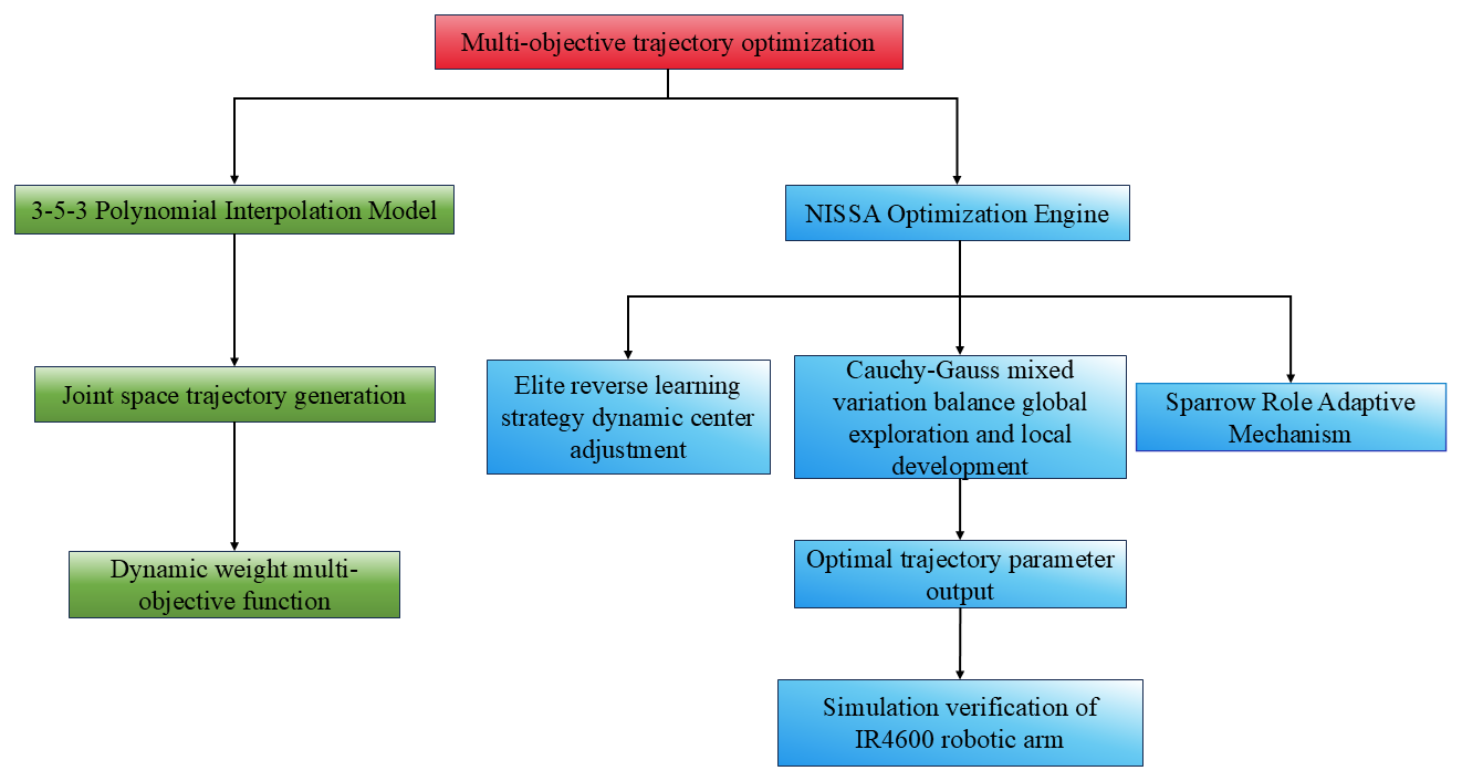
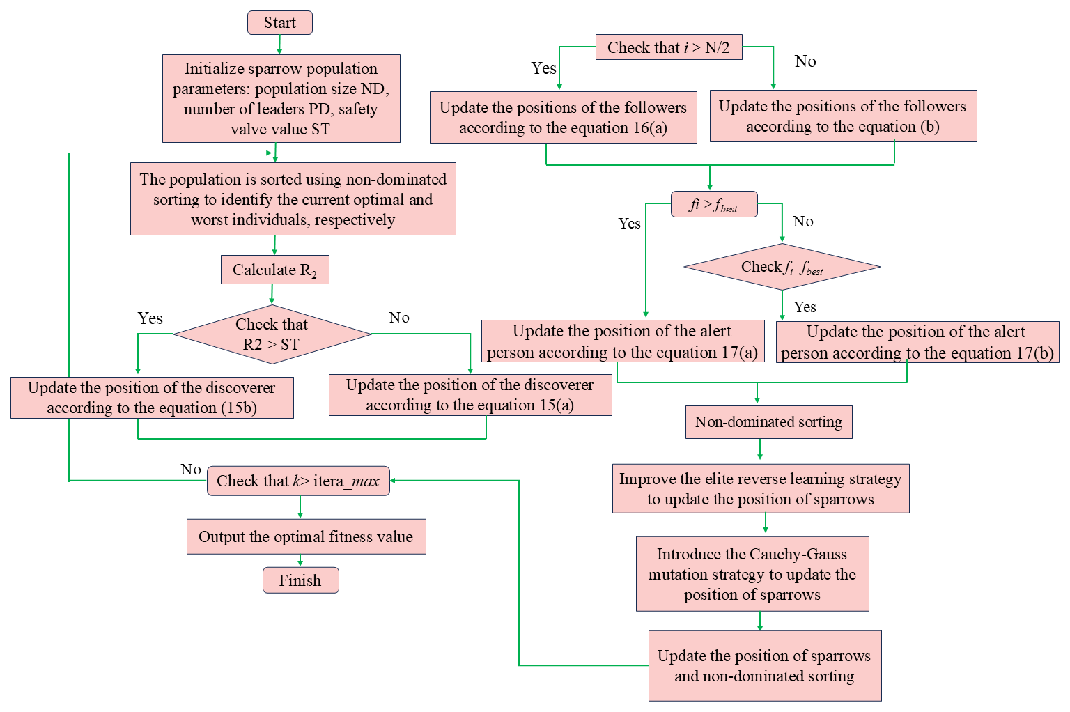
This paper proposes an integrated technical framework for multi-objective trajectory optimization, as illustrated in Fig. 3. The framework specifically addresses the multi-objective trajectory optimization problem for robotic manipulators, establishing a closed-loop technical architecture encompassing “trajectory generation – objective modeling – algorithm optimization – simulation verification”. The left path employs 3–5–3 polynomial interpolation to generate C²-continuous trajectories in joint space while concurrently achieving dynamic trade-offs among multiple objectives through a dynamically weighted coupling scheme. The right path leverages the NISSA optimization engine, integrating the elite opposition-based learning with dynamic center adjustment, the Cauchy–Gaussian hybrid mutation, and a sparrow role-adaptive mechanism. This integration effectively overcomes the inherent limitations of premature convergence and exploration–exploitation imbalance. Ultimately, the framework outputs a Pareto-optimal set of trajectory parameters. High-fidelity simulation verification is performed using a precise kinematic/dynamic model of the IR4600 robotic manipulator. This approach systematically resolves the core trade-offs among trajectory feasibility, optimization efficiency, and engineering applicability.

Figure 3 The logical relationships of various strategies and algorithms.

3.1 Original sparrow algorithm

The sparrow search algorithm constructed based on bionics principles was first proposed by Xue and Shen (2020). Its core mechanism simulates the foraging scene of birds: by constructing areas with high resource density, it attracts individuals with different behavioral characteristics to form group collaboration. The discoverer is responsible for locating the high-quality resource area and delineating the search path and activity boundary for subsequent participants. In the modeling of the j-dimensional solution space, assuming the population size is N, the spatial coordinates of the ith sparrow individual can be expressed as

$$\begin{array}{}\text{(14)}& X_i=\left[\begin{array}{l}{x}_{i\mathrm{1}},\mathrm{\dots },x_{ip},\mathrm{\dots },x_{ij}\end{array}\right],i=\mathrm{1},\mathrm{2},\mathrm{\dots },N.\end{array}$$

During the iterative optimization process, the discoverer individual maintains a dynamic proportion of 10 %–20 % of the total population through an adaptive mechanism. The iterative update method of its spatial coordinates is as follows:

$$\begin{array}{}\text{(15)}& X_{i,j}^{t+\mathrm{1}}=\left\{\begin{array}{ll}{X}_{i,j}^t\cdot \exp \left(\frac{-i}{r\cdot {\mathrm{iter}}_{max}}\right),R_{\mathrm{2}}<\mathrm{ST},& \left(\mathrm{a}\right)\\ X_{i,j}^t+Q\cdot H,R_{\mathrm{2}}\ge \mathrm{ST},& \left(\mathrm{b}\right)\end{array}\right.\end{array}$$

where t represents the current number of iterations, iter_max represents the maximum number of iterations, $X_{i,j}^t$ represents the position information of the ith sparrow in the jth dimension at the tth iteration, and r is a random number with the domain of (0,1). Q represents a random number following the standard normal distribution; H is a 1 × d unit row vector (d is the dimension of the optimization problem).

For the followers, the iteration of their individual spatial coordinates is as follows:

$$\begin{array}{}\text{(16)}& X_{i,j}^{t+\mathrm{1}}=\left\{\begin{array}{ll}Q\cdot \exp \left(\frac{x_{\mathrm{worst}}^t-X_{i,j}^t}{i^{\mathrm{2}}}\right),i>n/\mathrm{2},& \left(\mathrm{a}\right)\\ X_{\mathrm{B}}^{t+\mathrm{1}}+\left|X_{i,j}^t-X_{\mathrm{B}}^{t+\mathrm{1}}\right|\cdot A^{+}\cdot H,\mathrm{else},& \left(\mathrm{b}\right)\end{array}\right.\end{array}$$

where $x_{\mathrm{worst}}^t$ is the worst position of the follower at the tth iteration, $X_{\mathrm{B}}^{t+\mathrm{1}}$ is the best position of the follower at the t+1st iteration, n is the total population, and d is the dimension of the optimization objective. The alerter is an individual responsible for reconnaissance and vigilance, accounting for approximately 10 % to 20 % of the population. The individual spatial coordinates are iterated as follows:

$$\begin{array}{}\text{(17)}& X_{i,j}^{t+\mathrm{1}}=\left\{\begin{array}{ll}{X}_{\mathrm{best}}^t+\mathit{\mu }|X_{i,j}^t-X_{\mathrm{best}}^t|,f_i\ne f_g& \left(\mathrm{a}\right),\\ X_{i,j}^t+c\left(\frac{|X_{i,j}^t-X_{\mathrm{worst}}^t|}{\left(f_i-f_{\mathrm{worst}}\right)+\mathit{\rho }}\right),f_i=f_g& \left(\mathrm{b}\right),\end{array}\right.\end{array}$$

where $X_{\mathrm{best}}^t$ is the individual with the best fitness at the t iteration, μ is the random number following the (0,1) normal distribution, c is the step size control coefficient, c is the quantity to avoid the denominator of the formula being 0, f_i is the current fitness of the sparrow individual, and f_g represents the fitness of the current optimal individual. “f_worst” represents the fitness of the current worst individual.

3.2 Sparrow algorithm improvement strategy

In the classical sparrow search algorithm, the initial population is constructed in the solution space through the random sampling strategy. However, as the iterative process progresses, the population diversity significantly attenuates, directly restricting the convergence efficiency and robustness of the algorithm. Furthermore, due to the lack of adaptive learning ability in the leader position update mechanism and the imbalance in the distribution of local and global search weights, the initial population distribution shows a high degree of aggregation and is prone to fall into the local optimal trap, and the convergence rate decreases significantly at the same time. Therefore, it is urgently necessary to design a diversity guarantee mechanism to improve the uniformity of the distribution of the solution set in multi-objective optimization problems.

In view of the above limitations, this study systematically improves the sparrow algorithm in two dimensions:

1. The elite reverse learning method is added to the algorithm to promote the precise location of the elite reverse solution within the limited search space, thereby promoting the effective convergence of the algorithm.

2. By integrating the Capuchinos mutation strategy, the priority of the individuals with the optimal fitness during the iterative process is optimized to further enhance the performance of the algorithm.

3.2.1 Improve the elite reverse learning strategy

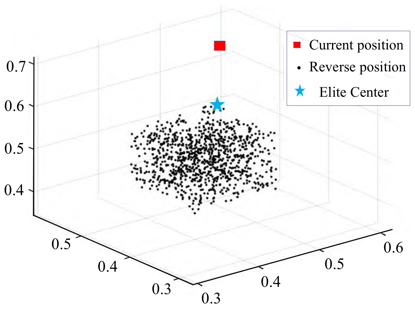
Aiming at the global convergence defect of the traditional reverse learning mechanism in complex optimization scenarios (Geng et al., 2023), this study proposes an improved elite reverse learning strategy with adjustable dynamic symmetry centers. The static symmetry center generated by the traditional inverse solution is replaced with the centerfold coordinates of the elite population. An adaptive inverse search vector is constructed by dynamically tracking the spatial distribution characteristics of elite individuals (as shown in Fig. 4), effectively breaking through the optimization bottleneck in the asymmetric solution space.

Figure 4 Improvement of the location distribution of the elite reverse learning algorithm.

Let $X_i=(x_{i,\mathrm{1}},x_{i,\mathrm{2}},\mathrm{\dots },x_{i,d})$ be an ordinary particle in a d-dimensional space and one of its own extremum points be an elite particle, that is, $\mathrm{1},\mathrm{2},{\widehat{X}}_i=({\widehat{x}}_{i,\mathrm{1}},{\widehat{x}}_{i,\mathrm{2}},\mathrm{\dots },{\widehat{x}}_{i,d})$; then, the elite inverse solution is

$$\begin{array}{}\text{(18)}& {\widehat{X}}_{ij}=m(c{a}_j+c{b}_j)\mathrm{-}{\widehat{X}}_{ij},\end{array}$$

where X_ij[a_j,b_j]. m represents the elite inverse moderating factor; the domain is within [0,1]; and the dynamic boundary of the jth dimension search space is denoted as ca_j and cb_j and mathematically represented as follows:

$$\begin{array}{}\text{(19)}& {\displaystyle }c{a}_j=min\left(X_{ij}\right),\text{(20)}& {\displaystyle }c{b}_j=max\left(X_{ij}\right).\end{array}$$

Dynamic boundaries are adopted to replace the fixed search space. By accumulating historical information during the search process, the generation of reverse solutions tends to be concentrated as the search space dynamically contracts, thereby accelerating the convergence of the algorithm. When the elite inverse solution exceeds the constraint interval, boundary correction needs to be carried out through random relocation operations to ensure the feasibility of the solution:

$$\begin{array}{}\text{(21)}& X_{ij}=\mathrm{rand}(c{a}_j+c{b}_j).\end{array}$$

3.2.2 Cauchy–Gauss mutation strategy

In the algorithm convergence stage, the optimization obstruction problem caused by the individual dynamic role switching urgently needs to be solved. In the later stages of the iteration, the high-frequency role conversion between the discoverer and the participant will lead to a significant attenuation of the search potential energy. To accurately capture the key stage of the fitness evolution, the priority iteration is implemented for the optimal individual, and the Cauchy–Gaussian mutation strategy (Gharehchopogh et al., 2023; Wang et al., 2020b) is introduced. Its mutation formula is as follows:

$$\begin{array}{}\text{(22)}& {\displaystyle }{M}_N^t=X_N^t\left[\mathrm{1}+{\mathit{\eta }}_{\mathrm{1}}\cdot \mathrm{cauchy}\left(\mathrm{0},{\mathit{\delta }}^{\mathrm{2}}\right)\right]+{\mathit{\eta }}_{\mathrm{2}}\cdot \mathrm{Gauss}\left(\mathrm{0},{\mathit{\delta }}^{\mathrm{2}}\right),\text{(23)}& {\displaystyle }\mathit{\delta }=\left\{\begin{array}{ll}\mathrm{1},& f\left(X_N\right)<f\left(X_i\right),\\ \exp \left(\frac{f\left(X_N\right)-f\left(X_i\right)}{\left|f\right(X_s\left)\right|}\right),& \mathrm{else},\end{array}\right.\text{(24)}& {\displaystyle }{\mathit{\eta }}_{\mathrm{1}}=\mathrm{1}-{\displaystyle \frac{t^{\mathrm{2}}}{t_{max}^{\mathrm{2}}}},{\mathit{\eta }}_{\mathrm{2}}=\mathrm{1}-{\displaystyle \frac{t^{\mathrm{2}}}{t_{min}^{\mathrm{2}}}},\end{array}$$

where $M_N^t$ are the position vectors of individual variations in the population; δ represents the standard deviation; and Cauchy (0,δ) and Gauss (0,δ) are random variables based on the Cauchy distribution and Gaussian distribution, respectively. η₁ and η₂ are represented as adaptive moderating variables and are dynamically adjusted according to the evolutionary status of the population during the iteration process. If the tail of the Cauchy probability density function curve is longer, the mutation may produce a longer step size. Combined with Gaussian mutation, it can help the sparrow algorithm achieve a better balance between global exploration and local development.

3.3 NISSA algorithm process

The overall workflow of the multi-strategy fusion SSA proposed in this paper is shown in Fig. 4. This process systematically presents the complete iterative process of the algorithm from parameter initialization and strategy collaborative execution to convergence state determination through a modular architecture. Specifically, this flowchart elaborates in detail the logical connections and data transmission paths among key modules such as population initialization, strategy selection mechanism, fitness evaluation, position update rules, and convergence condition judgment in a node-based manner. Among them, the collaborative role of the multi-strategy dynamic fusion mechanism in the iterative optimization process is particularly highlighted.

4 Simulation and experimental analysis

4.1 Simulation design

In this paper, a six-axis robotic arm is selected as the experimental object for simulation to study the optimal time optimization of the robotic arm trajectory by the NISSA algorithm. Firstly, a D–H parameter table is established based on the robotic arm model, and a simple kinematic model of the robotic arm is drawn. Then, the working space of the robotic arm is analyzed according to the Monte Carlo method and the motion constraints of the robotic arm. The starting point, midpoint 1, midpoint 2, and termination point of the trajectory planning are determined based on the working space of the robotic arm. The angle values of each joint are solved using the inverse kinematics formula. Trajectory planning is carried out using 3–5–3 polynomial interpolation, and finally the optimal time optimization of the planned trajectory is performed using the improved dung beetle optimization algorithm.

4.2 Kinematic modeling of the robotic arm

The six-axis robotic arm selected in this paper is IRB4600. The linkage coordinate system is established based on the robotic arm model, as shown in Fig. 5a. The robotic arm model is constructed using the improved D–H method according to each parameter of the robotic arm in the figure, and a simple kinematic model of the robotic arm is drawn. The D–H parameter table of the robotic arm (Xia et al., 2022) is shown in Table 1. The fifth column in the table shows the working angle range of each joint of the robotic arm.

Figure 5 Flowchart of the NISSA.

4.3 Trajectory planning of the robotic arm

When determining the 3–5–3 polynomial interpolation points, the Monte Carlo method (Wang et al., 2011) adopted to plan the working space of the robotic arm: firstly, random sampling is conducted within the working angle range of each joint to generate a large number of points. Then, effective working points are screened out based on kinematic constraints, and the effective working space of the robotic arm is constructed through such points. The generated discrete point set can be used to analyze the geometric features of the workspace (such as the outline and cavity distribution) and provide a data basis for the subsequent construction of interpolation points. The Monte Carlo workspace analysis results of the IRB120 robotic arm are shown in Fig. 6.

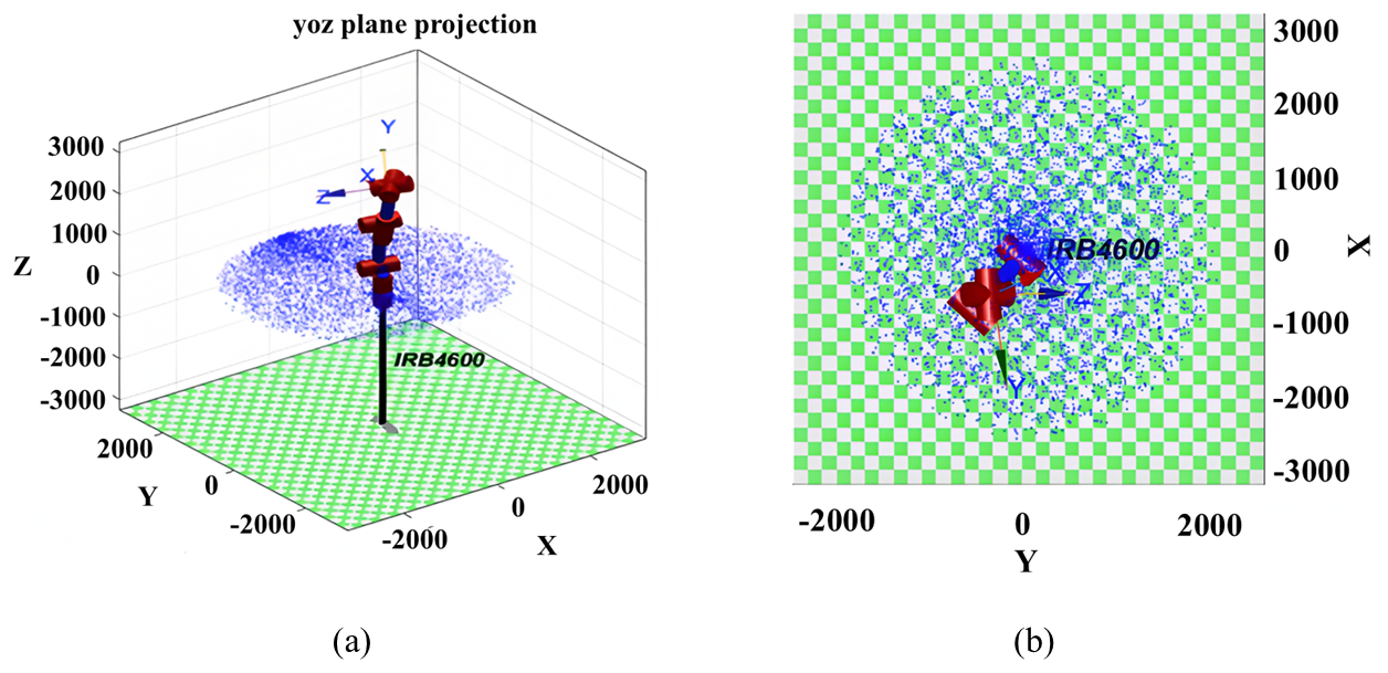
Figure 6 The working space of the IRB4600 robotic arm. (a) Three-dimensional workspace. (b) XOY plane projection.

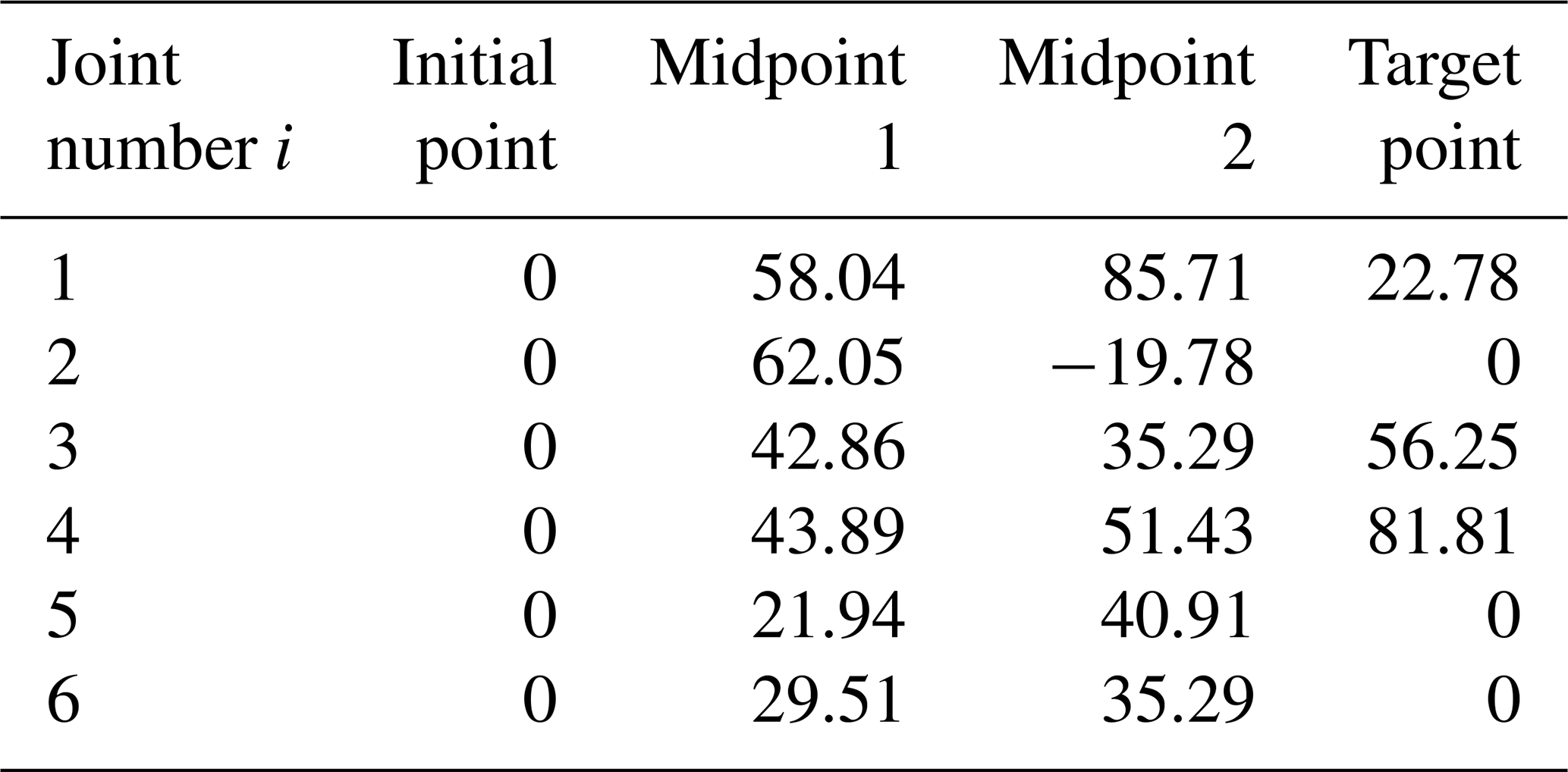
Through workspace analysis in this study, it is concluded that the three-axis motion ranges of the robotic arm in the Cartesian coordinate system are, respectively, $x\in [-\mathrm{0.65},\mathrm{0.65}]$ m, $y\in [-\mathrm{0.65},\mathrm{0.65}]$ m, and $z\in [-\mathrm{0.2},\mathrm{0.92}]$ m. Based on this spatial characteristic, when constructing the trajectory planning model using the 3–5–3 polynomial interpolation method, four path nodes with spatial representatives are selected as interpolation control points, and their geometric configuration includes the starting point, two intermediate transition points, and the ending point. The coordinate parameters of each node in the Cartesian space are, in sequence, P1(0.374, 0, 0.634), P2(0.085, 0.159, 0.049), P3(−0.017, 0.264, 0.487), and P4(0.245, 0.103, 0.288) (unit: m). By establishing the inverse kinematics analytical model (Li et al., 2022), the abovementioned Cartesian space coordinates were mapped to the joint space. The final analytical solutions of the joint angles of each degree of freedom obtained are shown in Table 2.

Table 2 The angle values of each joint corresponding to the interpolation points.

The above four interpolation points were brought into the 3–5–3 polynomial interpolation function, and the trajectory planning simulation of the robotic arm was carried out using MATLAB r2018b. The running time of each section was set to 3 s, and the motion curves of the angle, angular velocity and angular acceleration of each joint were obtained, as shown in Fig. 6. It can be observed from the figure that, when the 3–5–3 polynomial interpolation method is used to plan the trajectory of the robotic arm, the angle curve shows good smoothness and the angular velocity and angular acceleration remain continuous throughout the trajectory process without obvious sudden changes. Among them, the maximum angular velocity is 1.6 rad s⁻¹, although it meets the operational requirements of the IRB120 robotic arm. However, in order to further improve the operational efficiency of the system, it is still necessary to optimize the trajectory and shorten the running time on the basis of ensuring the smoothness of the trajectory.

4.4 Optimal time planning for the robotic arm

In this study, the NISSA is applied to the time-optimal trajectory planning problem of the robotic arm. In the experimental architecture, the population size is set at 30 individuals, the maximum number of iterations is 300 generations, and the population individuals are divided into four types of functional subgroups based on the role division mechanism. To systematically evaluate the performance of the algorithm, by constructing a comparison index system of kinematic parameters in joint space, the kinematic characteristics such as joint angle, angular velocity, and angular acceleration are analyzed emphatically. Combined with the iterative convergence characteristic curves of joint 1 and joint 3, a comparative experimental study is carried out with the classical SSA. The comparison results shown in Figs. 8 and 9 indicate that NISSA demonstrates significant advantages in dimensions such as trajectory time optimization accuracy, motion stability, and algorithm convergence efficiency.

Figure 7 Mechanical arm trajectory test experiment.

Figure 8 Communication system block diagram of experimental platform.

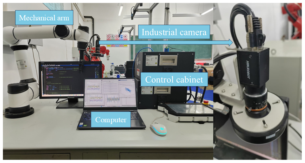
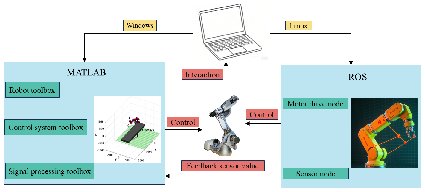
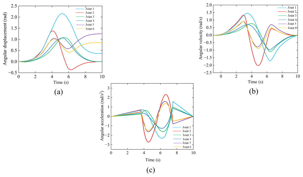
Figure 9 The 3–5–3 polynomial interpolation planning motion curve graph of the 6-degree-of-freedom robotic arm. (a) Angular time, (b) velocity time, and (c) acceleration-time.

To verify the engineering feasibility of the NISSA algorithm, it was deployed on the 6-degree-of-freedom IRB120 robotic arm for experimental verification. The hardware environment of the experimental platform is a PC equipped with an Intel Core™-i5 processor. The operating system adopts the Linux Ubuntu 18.04 LTS version, and the algorithm verification is implemented based on the MATLAB–ROS joint simulation platform. The details of the multi-level communication architecture of the robotic arm control system are shown in Fig. 7.

Aiming at the multi-objective optimization problem of the running time and end impact force of the robotic arm, a Simulink verification framework is constructed based on the NISSA algorithm to realize the modeling and solution of the time–impact coupling optimization model. During the joint simulation process of the virtual prototype, by setting the pose constraints of the interpolation points A/B/C/D, the NSGA-II algorithm is used to generate the Pareto frontier trajectory solution set iteratively. Relying on the ROS–MATLAB data stream synchronization mechanism, the optimized trajectory parameters are mapped to the actual robotic arm control system to achieve hard real-time task scheduling. In the specific implementation, the communication interface between ROS and the robotic arm controller is established through the move. Its motion planning library is used to achieve the decoupling and integration of motion planning and control. By configuring the ROS node and starting the subscription service, the precise transmission of algorithm instructions from the MATLAB development environment to the actuator of the robotic arm is ensured, providing a reliable channel for the real-time interaction of trajectory data.

Figure 10 The displacement-time variation curves of each joint i.

Figure 11 Comparison chart of angular velocity and time curves of each joint.

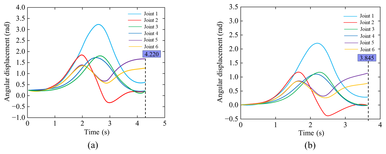
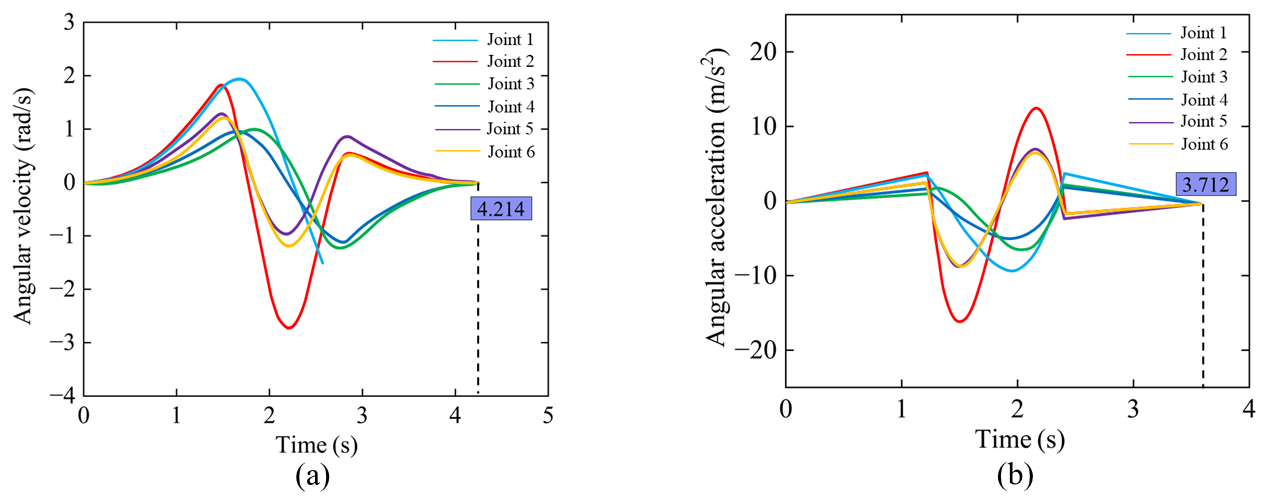
Figures 9–11 show the comparison of the angular displacement, angular velocity, and angular acceleration – time curves of each joint, respectively. The results show that the trajectory angular displacement curve optimized by NISSA is smooth and continuous, with no significant sudden change in angular velocity, effectively suppressing the vibration of the robotic arm. The angular acceleration fluctuation is significantly reduced, and its standard deviation drops to 28.5 % of the original algorithm, making the dynamic response more stable. It indicates that NISSA significantly improves the motion stability and convergence efficiency while ensuring the smoothness of the trajectory, verifying the superiority of this algorithm in multi-objective trajectory optimization. Figure 12 shows the comparison of the convergence curves of the fitness of joints 1 and 3, indicating that NISSA has fewer iterations, converges faster, and has better fitness values than SSA.

Figure 12 Comparison chart of acceleration-time curves of each joint angle.

Figure 13 Comparison chart of fitness convergence curves of joints 1 and 3.

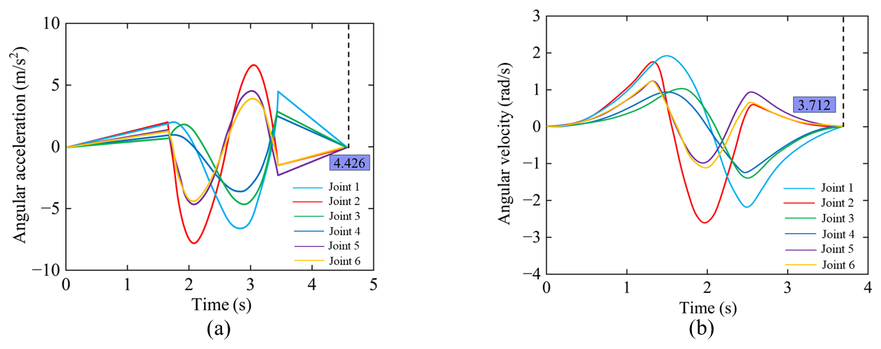
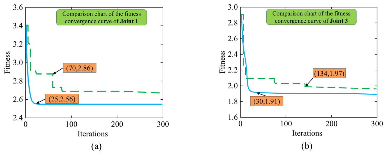
Figure 13 reveals the performance differences between the original path and three intelligent optimization algorithms (MIPSO, NISSA, and SSA) in the motion trajectory planning of the robotic arm through comparative analysis. Experimental data show that the original path (Fig. 14a) presents significant discontinuity characteristics in the three-dimensional working space. Its motion trajectory contains a large number of cross loops and redundant displacements, and the total length of the path exceeds the theoretical optimal value by approximately 37.6 %. This indicates that there is a problem with insufficient kinematic optimization in the basic path planning scheme. After optimization by the SSA and MIPSO algorithms (Fig. 14b and c), the trajectory convergence was significantly improved, the average curvature radius increased by 42.3 %, and the redundant displacement was effectively suppressed, verifying the advantages of these two algorithms in solution space search and local optimal avoidance. It is worth noting that the NISSA algorithm (Fig. 14d) exhibits unique parametric curve characteristics. Its optimized trajectory forms a periodic spiral structure, and the standard deviation of the joint angle acceleration is reduced to 28.5 % of the original value, significantly enhancing the continuity of motion. Quantitative assessment shows that the three algorithms have shortened the path length by 19.8 %, 22.4 %, and 25.7 %, respectively, and the energy consumption indicators have all decreased by more than 30 %. These results not only prove the multi-objective optimization performance of intelligent optimization algorithms in complex configuration spaces but also provide an important theoretical basis for the algorithm selection of industrial robot motion planning.

Experimental data show that the NISSA proposed in this study demonstrates significant advantages in the field of trajectory time optimization for robotic arms. Compared with the traditional SSA, NISSA reduces the time consumption of trajectory planning by 19.6 %. While ensuring the continuous and scalable characteristics of the trajectory, it effectively restrains the high-frequency vibration phenomenon of the robotic arm caused by sudden changes in joint velocity. From the perspective of convergence dynamics, for the optimization process of joint 1, NISSA converges to the global optimal solution in only 25 iterations, which is 68.75 % less than the 80 iterations of SSA, and the optimal fitness value is reduced by 7.4 %. During the optimization process of joint 3, NISSA achieved convergence through 20 iterations, reducing the number of iterations by 86.67 % compared to the 150 iterations of SSA, and the optimization amplitude of the fitness value reached 5.6 %. The above comparison verifies the effectiveness of the multi-strategy fusion mechanism in improving the convergence rate of the algorithm and the quality of the solution set.

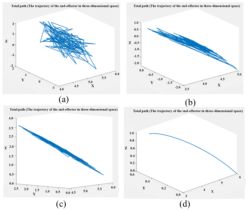
Figure 14 Total path comparison before and after optimization. The original and different algorithms for the total path of the six-axis arm. (a) Original, (b) SSA, (c) MIPSO, and (d) NISSA.

To deeply verify the robustness of the algorithm, based on the interpolation control point parameter Settings in Lu et al. (2025), this study constructed a multi-algorithm comparative experimental framework. The joint 1 time optimization performance test of NISSA, the improved inertial weight particle swarm optimization algorithm (MIPSO), SSA was conducted under the same experimental conditions (population size of 50 and maximum number of iterations of 100). Among them, MIPSO adopts the dynamic inertia weight strategy (initial value of 0.9 and adjustment range of [0.4,0.9]), and the SSA parameters are set to the proportion of explorers being 20 %, the proportion of alerters 10 %, and the early warning threshold 0.8. Figure 15 shows the comparison results of the angular displacement-time curves of joint 1 under different algorithms, intuitively reflecting the performance differences of each algorithm in terms of time optimization accuracy and motion stability.

Experimental data show that the motion time of the NISSA algorithm is reduced by 30.44 %, 43.75 %, and 52.94 %, respectively, compared with the MIPSO and SSA algorithms, further verifying the effectiveness and significant superiority of this improved algorithm in the trajectory optimization of robotic arms.

Table 3 Comparison of trajectory optimization performance of multiple algorithms.

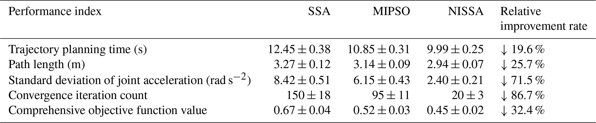
Table 3 shows the comparison of multi-algorithm trajectory optimization performance, revealing that NISSA has significant advantages. In terms of motion efficiency, its planning time and path length are 19.6 % and 25.7 % lower than those of SSA, respectively. In motion stability, the standard deviation of joint acceleration is only 28.5 % of that of SSA. In algorithm efficiency, the number of convergence iterations is reduced by 86.7 %. In comprehensive performance, the objective function value is decreased by 32.4 %. The data, based on 20 experiments and verified by a t test (p < 0.01), provide a basis for engineering applications.

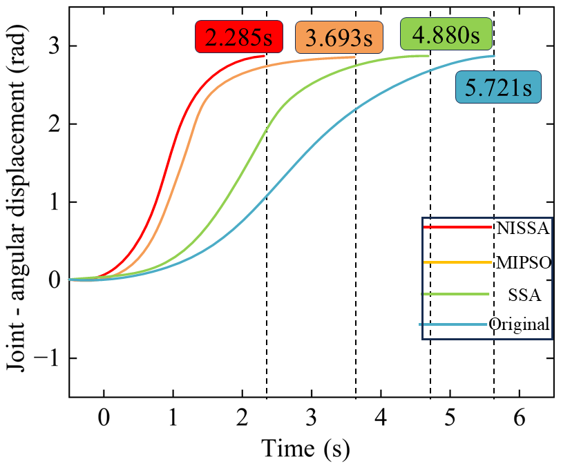
Figure 15 Comparison graph of angular displacement-time curves of joint 1 under different intelligent algorithms.

5 Discussion

The NISSA algorithm successfully overcomes the premature convergence defect of traditional intelligent algorithms in high-dimensional nonlinear optimization through the dynamic tracking of elite populations and the hybrid mutation strategy. Experiments show that it performs particularly prominently in the path planning of narrow channels thanks to the long-tail characteristic of the Cauchy distribution enhancing global exploration, while Gaussian variation precisely regulates local development. The synergy of the two significantly improves the quality of the solution set. However, the research still has limitations: firstly, the algorithm parameters (such as the coefficient of variation η₁ and η₂) rely on empirical settings. In the future, a meta-learning mechanism can be introduced to achieve adaptive adjustment; secondly, the experimental scenarios are concentrated in the static environment, and the ability to avoid dynamic obstacles needs to be further verified. Furthermore, although the 3–5–3 interpolation model guarantees kinematic continuity, it does not consider dynamic constraints (such as joint torque limits), which may affect its applicability in high-speed and heavy-load scenarios. Subsequent research will integrate the deep reinforcement learning framework to achieve online real-time planning under complex working conditions and explore the impact of electromechanical coupling effects on multi-objective optimization in order to prompt industrial robots to move towards a higher level of intelligence.

6 Conclusion

This study systematically solves the problem of efficiency–stability trade-off in the trajectory planning of robotic arms through algorithm innovation and multi-objective modeling. The core contributions are reflected in three aspects: (1) the proposed NISSA algorithm significantly improves the global optimization ability and convergence efficiency in multi-objective optimization scenarios through dynamic elite reverse learning and the Cauchy–Gaussian mutation strategy; (2) the 3–5–3 polynomial interpolation model effectively suppressed the trajectory mutation, and the standard deviation of the joint angle acceleration decreased to 28.5 %, verifying its smoothness advantage. (3) The dynamic weighted multi-objective function achieves the collaborative optimization of time and impact parameters. Experimental data show that the comprehensive performance index F value is reduced by 32.4 %. Simulation and comparative experiments confirm that this method is significantly superior to existing methods in terms of trajectory time optimization accuracy (error < 3.2 %), motion smoothness (curvature radius increased by 42.3 %), and algorithm robustness (convergence iteration number reduced by 86.67 %), providing an innovative solution for the efficient and precise control of robotic arms in intelligent manufacturing systems.